A Siamese Deep Forest

Abstract

A Siamese Deep Forest (SDF) is proposed in the paper. It is based on the Deep Forest or gcForest proposed by Zhou and Feng and can be viewed as a gcForest modification. It can be also regarded as an alternative to the well-known Siamese neural networks. The SDF uses a modified training set consisting of concatenated pairs of vectors. Moreover, it defines the class distributions in the deep forest as the weighted sum of the tree class probabilities such that the weights are determined in order to reduce distances between similar pairs and to increase them between dissimilar points. We show that the weights can be obtained by solving a quadratic optimization problem. The SDF aims to prevent overfitting which takes place in neural networks when only limited training data are available. The numerical experiments illustrate the proposed distance metric method.

Keywords: classification, random forest, decision tree, Siamese, deep learning, metric learning, quadratic optimization

1 Introduction

One of the important machine learning tasks is to compare pairs of objects, for example, pairs of images, pairs of data vectors, etc. There are a lot of approaches for solving the task. One of the approaches is based on computing a corresponding pairwise metric function which measures a distance between data vectors or a similarity between the vectors. This approach is called the metric learning [1, 14, 27]. It is pointed out by Bellet et al. [1] in their review paper that the metric learning aims to adapt the pairwise real-valued metric function, for example, the Mahalanobis distance or the Euclidean distance, to a problem of interest using the information provided by training data. A detailed description of the metric learning approaches is also represented by Le Capitaine [5] and by Kulis [14]. The basic idea underlying the metric learning solution is that the distance between similar objects should be smaller than the distance between different objects.

Suppose there is a training set $S$ $=\{(\mathbf{x}_{i},\mathbf{x}_{j},y_{ij}),\ (i,j)\in K\}$ consisting of $N$ pairs of examples $\mathbf{x}_{i}\in\mathbb{R}^{m}$ and $\mathbf{x}_{j}\in\mathbb{R}^{m}$ such that a binary label $y_{ij}\in\{0,1\}$ is assigned to every pair $(\mathbf{x}_{i},\mathbf{x}_{j})$. If two data vectors $\mathbf{x}_{i}$ and $\mathbf{x}_{j}$ are semantically similar or belong to the same class of objects, then $y_{ij}$ takes the value $0$. If the vectors correspond to different or semantically dissimilar objects, then $y_{ij}$ takes the value $1$. This implies that the training set $S$ can be divided into two subsets. The first subset is called the similar or positive set and is defined as

$$\mathcal{S}=\{(\mathbf{x}_{i},\mathbf{x}_{j}):\mathbf{x}_{i}\text{ and }\mathbf{x}_{j}\ \text{are semantically similar and }y_{ij}=0\}.$$

The second subset is the dissimilar or negative set. It is defined as

$$\mathcal{D}=\{(\mathbf{x}_{i},\mathbf{x}_{j}):\mathbf{x}_{i}\text{ and }\mathbf{x}_{j}\ \text{are semantically dissimilar and }y_{ij}=1\}.$$

If we have two observation vectors $\mathbf{x}_{i}\in\mathbb{R}^{m}$ and $\mathbf{x}_{j}\in\mathbb{R}^{m}$ from the training set, then the distance $d(\mathbf{x}_{i},\mathbf{x}_{j})$ should be minimized if $\mathbf{x}_{i}$ and $\mathbf{x}_{j}$ are semantically similar, and it should be maximized between dissimilar $\mathbf{x}_{i}$ and $\mathbf{x}_{j}$. The most general and popular real-valued metric function is the squared Mahalanobis distance $d_{M}^{2}(\mathbf{x}_{i},\mathbf{x}_{j})$ which is defined for vectors $\mathbf{x}_{i}$ and $\mathbf{x}_{j}$ as

$$d_{M}^{2}(\mathbf{x}_{i},\mathbf{x}_{j})=(\mathbf{x}_{i}-\mathbf{x}_{j})^{\mathrm{T}}M(\mathbf{x}_{i}-\mathbf{x}_{j}).$$

Here $M\in\mathbb{R}^{m\times m}$ is a symmetric positive semi-defined matrix. If $\mathbf{x}_{i}$ and $\mathbf{x}_{j}$ are random vectors from the same distribution with covariance matrix $C$, then $M=C^{-1}$. If $M$ is the identity matrix, then $d_{M}^{2}(\mathbf{x}_{i},\mathbf{x}_{j})$ is the squared Euclidean distance.

Given subsets $\mathcal{S}$ and $\mathcal{D}$, the metric learning optimization problem can be formulated as follows:

$$M^{\ast}=\arg\min_{M}\left[J(M,\mathcal{D},\mathcal{S})+\lambda\cdot R(M)\right],$$

where $J(M,\mathcal{D},\mathcal{S})$ is a loss function that penalizes violated constraints; $R(M)$ is some regularizer on $M$; $\lambda\geq 0$ is the regularization parameter.

There are many useful loss functions $J$ which take into account the condition that the distance between similar objects should be smaller than the distance between different objects. These functions define a number of learning methods. It should be noted that the learning methods using the Mahalanobis distance assume some linear structure of data. If this is not valid, then the kernelization of linear methods is one of the possible ways for solving the metric learning problem. Bellet et al. [1] review several approaches and algorithms to deal with nonlinear forms of metrics. In particular, these are the Support Vector Metric Learning algorithm provided by Xu et al. [26], the Gradient-Boosted Large Margin Nearest Neighbors method proposed by Kedem et al. [12], the Hamming Distance Metric Learning algorithm provided by Norouzi et al. [19].

A powerful implementation of the metric learning dealing with non-linear data structures is the so-called Siamese neural network introduced by Bromley et al. [4] in order to solve signature verification as a problem of image matching. This network consists of two identical sub-networks joined at their outputs. The two sub-networks extract features from two input examples during training, while the joining neuron measures the distance between the two feature vectors. The Siamese architecture has been exploited in many applications, for example, in face verification [7], in the one-shot learning in which predictions are made given only a single example of each new class [13], in constructing an inertial gesture classification [2], in deep learning [23], in extracting speaker-specific information [6], for face verification in the wild [11]. This is only a part of successful applications of Siamese neural networks. Many modifications of Siamese networks have been developed, including fully-convolutional Siamese networks [3], Siamese networks combined with a gradient boosting classifier [15], Siamese networks with the triangular similarity metric [27].

One of the difficulties of the Siamese neural network as well as other neural networks is that limited training data lead to overfitting when training neural networks. Many different methods have been developed to prevent overfitting, for example, dropout methods [21] which are based on combination of the results of different networks by randomly dropping out neurons in the network. A very interesting new method which can be regarded as an alternative to deep neural networks is the deep forest proposed by Zhou and Feng [28] and called the gcForest. In fact, this is a multi-layer structure where each layer contains many random forests, i.e., this is an ensemble of decision tree ensembles. Zhou and Feng [28] point out that their approach is highly competitive to deep neural networks. In contrast to deep neural networks which require great effort in hyperparameter tuning and large-scale training data, gcForest is much easier to train and can perfectly work when there are only small-scale training data. The deep forest solves tasks of classification as well as regression. Therefore, by taking into account its advantages, it is important to modify it in order to develop a structure solving the metric learning task. We propose the so-called Siamese Deep Forest (SDF) which can be regarded as an alternative to the Siamese neural networks and which is based on the gcForest proposed by Zhou and Feng [28] and can be viewed as its modification. Three main ideas underlying the SDF can be formulated as follows:

1. We propose to modify training set by using concatenated pairs of vectors.

2. We define the class distributions in the deep forest as the weighted sum of the tree class probabilities where the weights are determined in order to reduce distances between semantically similar pairs of examples and to increase them between dissimilar pairs. The weights are training parameters of the SDF.

3. We apply the greedy algorithm for training the SDF, i.e., the weights are successively computed for every layer or level of the forest cascade.

We consider the case of the weakly supervised learning [1] when there are no information about the class labels of individual training examples, but only information in the form of sets $\mathcal{S}$ and $\mathcal{D}$ is provided, i.e., we know only semantic similarity of pairs of training data. However, the case of the fully supervised learning when the class labels of individual training examples are known can be considered in the same way.

It should be noted that the SDF cannot be called Siamese in the true sense of the word. It does not consist of two gcForests like the Siamese neural network. However, its aim coincides with the Siamese network aim. Therefore, we give this name for the gcForest modification.

The paper is organized as follows. Section 2 gives a very short introduction into the Siamese neural networks. A short description of the gcForest proposed by Zhou and Feng [28] is given in Section 3. The ideas underlying the SDF are represented in Section 4 in detail. A modification of the gcForest using the weighted averages, which can be regarded as a basis of the SDF is provided in Section 5. Algorithms for training and testing the SDF are considered in Section 6. Numerical experiments with real data illustrating cases when the proposed SDF outperforms the gcForest are given in Section 7. Concluding remarks are provided in Section 8.

2 Siamese neural networks

Before studying the SDF, we consider the Siamese neural network which is an efficient and popular tool for dealing with data of the form $\mathcal{S}$ and $\mathcal{D}$. It will be a basis for constructing the SDF.

A standard architecture of the Siamese network given in the literature (see, for example, [7]) is shown in Fig. 1. Let $\mathbf{x}_{i}$ and $\mathbf{x}_{j}$ be two data vectors corresponding to a pair of elements from a training set, for example, images. Suppose that $f$ is a map of $\mathbf{x}_{i}$ and $\mathbf{x}_{j}$ to a low-dimensional space such that it is implemented as a neural network with the weight matrix $W$. At that, parameters $W$ are shared by two neural networks $f(\mathbf{x}_{1})$ and $f(\mathbf{x}_{2})$ denoted as $E_{1}$ and $E_{2}$ and corresponding to different input vectors, i.e., they are the same for the two neural networks. The property of the same parameters in the Siamese neural network is very important because it defines the corresponding training algorithm. By comparing the outputs $\mathbf{h}_{i}=f(\mathbf{x}_{i})$ and $\mathbf{h}_{j}=f(\mathbf{x}_{j})$ using the Euclidean distance $d(\mathbf{h}_{i},\mathbf{h}_{j})$, we measure the compatibility between $\mathbf{x}_{i}$ and $\mathbf{x}_{j}$.

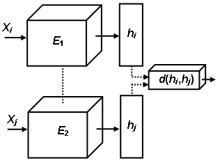
Figure 1: An architecture of the Siamese neural network

If we assume for simplicity that the neural network has one hidden layer, then there holds

$$\mathbf{h}=\sigma(W\mathbf{x}+b).$$

Here $\sigma(z)$ is an activation function; $W$ is the weight $p\times M$ matrix such that its element $w_{ij}$ is the weight of the connection between unit $j$ in the input layer and unit $i$ in the hidden layer, $i=1,...,p$, $j=1,...,M$; $b=(b_{1},...,b_{p})$ is a bias vector; $\mathbf{h}=(h_{1},...,h_{p})$ is the vector of neuron activations, which depends on the input vector $\mathbf{x}$.

The Siamese neural network is trained on pairs of observations by using specific loss functions, for example, the following contrastive loss function:

$$l(\mathbf{x}_{i},\mathbf{x}_{j},y_{ij})=\left\{\begin{array}[c]{cc}\left\|\mathbf{h}_{i}-\mathbf{h}_{j}\right\|_{2}^{2},&y_{ij}=0,\\ \max(0,\tau-\left\|\mathbf{h}_{i}-\mathbf{h}_{j}\right\|_{2}^{2}),&y_{ij}=1,\end{array}\right.$$ (1)

where $\tau$ is a predefined threshold.

Hence, the total error function for minimizing is defined as

$$J(W,b)=\sum\nolimits_{i,j}l(\mathbf{x}_{i},\mathbf{x}_{j},y_{ij})+\mu R(W,b).$$

Here $R(W,b)$ is a regularization term added to improve generalization of the neural network, $\mu$ is a hyper-parameter which controls the strength of the regularization. The above problem can be solved by using the stochastic gradient descent scheme.

3 Deep Forest

According to [28], the gcForest generates a deep forest ensemble, with a cascade structure. Representation learning in deep neural networks mostly relies on the layer-by-layer processing of raw features. The gcForest representational learning ability can be further enhanced by the so-called multi-grained scanning. Each level of cascade structure receives feature information processed by its preceding level, and outputs its processing result to the next level. Moreover, each cascade level is an ensemble of decision tree forests. We do not consider in detail the Multi-Grained Scanning where sliding windows are used to scan the raw features because this part of the deep forest is the same in the SDF. However, the most interesting component of the gcForest from the SDF construction point of view is the cascade forest.

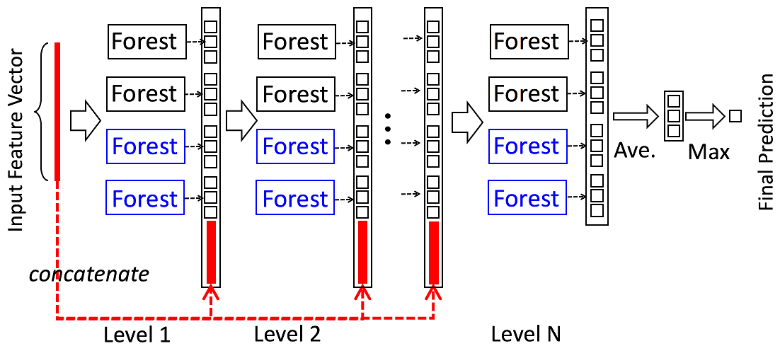
Figure 2: The architecture of the cascade forest [28]

Given an instance, each forest produces an estimate of class distribution by counting the percentage of different classes of examples at the leaf node where the concerned instance falls into, and then averaging across all trees in the same forest. The class distribution forms a class vector, which is then concatenated with the original vector to be input to the next level of cascade. The usage of the class vector as a result of the random forest classification is very similar to the idea underlying the stacking method [24]. The stacking algorithm trains the first-level learners using the original training data set. Then it generates a new data set for training the second-level learner (meta-learner) such that the outputs of the first-level learners are regarded as input features for the second-level learner while the original labels are still regarded as labels of the new training data. In fact, the class vectors in the gcForest can be viewed as the meta-learners. In contrast to the stacking algorithm, the gcForest simultaneously uses the original vector and the class vectors (meta-learners) at the next level of cascade by means of their concatenation. This implies that the feature vector is enlarged and enlarged after every cascade level. The architecture of the cascade proposed by Zhou and Feng [28] is shown in Fig. 2. It can be seen from the figure that each level of the cascade consists of two different pairs of random forests which generate 3-dimensional class vectors concatenated each other and with the original input. After the last level, we have the feature representation of the input feature vector, which can be classified in order to get the final prediction. Zhou and Feng [28] propose to use different forests at every level in order to provide the diversity which is an important requirement for the random forest construction.

4 Three ideas underlying the SDF

The SDF aims to function like the standard Siamese neural network. This implies that the SDF should provide large distances between semantically similar pairs of vectors and small distances between dissimilar pairs. We propose three main ideas underlying the SDF:

1. Denote the set indices of all pairs $\mathbf{x}_{i}$ and $\mathbf{x}_{j}$ as $K=\{(i,j)\}$ We train every tree by using the concatenation of two vectors $\mathbf{x}_{i}$ and $\mathbf{x}_{j}$ such that the class $y_{ij}\in\{0,1\}$ is defined by the semantical similarity of the vectors. In fact, the trees are trained on the basis of two classes and reflect the semantical similarity of pairs, but not classes of separate examples. With this concatenation, we define a new set of classes such that we do not need to know separate classes for $\mathbf{x}_{i}$ or for $\mathbf{x}_{j}$. As a result, we have a new training set $R=\{(\mathbf{x}_{i},\mathbf{x}_{j}),y_{ij}),\ (i,j)\in K\}$ and exploit only the information about the semantical similarity. The concatenation is not necessary when the classes of training elements are known, i.e., we have a set of labels $\{y_{1},...,y_{n}\}$. In this case, only the second idea can be applied.

2. We partially use some modification of ideas provided by Xiong et al. [25] and Dong et al. [8]. In particular, Xiong et al. [25] considered an algorithm for solving the metric learning problem by means of the random forests. The proposed metric is able to implicitly adapt its distance function throughout the feature space. Dong et al. [8] proposed a random forest metric learning (RFML) algorithm, which combines semi-multiple metrics with random forests to better separate the desired targets and background in detecting and identifying target pixels based on specific spectral signatures in hyperspectral image processing. A common idea underlying the metric learning algorithms in [25] and [8] is that the distance measure between a pair of training elements $\mathbf{x}_{i},\mathbf{x}_{j}$ for a combination of trees is defined as average of some special functions of the training elements. For example, if a random forest is a combination of $T$ decision trees $\{f_{t}(\mathbf{x}),t=1,...,T\}$, then the distance measure is

   $$d(\mathbf{x}_{i},\mathbf{x}_{j})=T^{-1}\sum_{t=1}^{T}f_{t}(\psi(\mathbf{x}_{i},\mathbf{x}_{j})).$$

   Here $\psi(\mathbf{x}_{i},\mathbf{x}_{j})$ is a mapping function which is specifically defined in [25] and [8]. We combine the above ideas with the idea of probability distributions of classes provided in [28] in order to produce a new feature vector after every level of the cascade forest. According to [28], each forest of a cascade level produces an estimate of the class probability distribution by counting the percentage of different classes of training examples at the leaf node where the concerned instance falls into, and then averaging across all trees in the same forest. Our idea is to define the forest class distribution as a weighted sum of the tree class probabilities. At that, the weights are computed in an optimal way in order to reduce distances between similar pairs and to increase them between dissimilar points.

   The obtained weights are very similar to weights of the neural network connections between neurons, which are also computed during training the neural network. The trained values of weights in the SDF are determined in accordance with a loss function defining properties of the SDF or the neural network. Due to this similarity, we will call levels of the cascade as layers sometimes.

   It should be also noted that the first idea can be sufficient for implementing the SDF because the additional features (the class vectors) produced by the previous cascade levels partly reflect the semantical similarity of pairs of examples. However, in order to enhance the discriminative capability of the SDF, we modify the corresponding class distributions.

3. We apply the greedy algorithm for training the SDF that is we train separately every level starting from the first level such that every next level uses results of training at the previous level. In contrast to many neural networks, the weights considered above are successively computed for every layer or level of the forest cascade.

5 The SDF construction

Let us introduce notations for indices corresponding to different deep forest components. The indices and their sets of values are shown in Table 1. One can see from Table 1, that there are $Q$ levels of the deep forest or the cascade, every level contains $M_{q}$ forests such that every forest consists of $T_{k,q}$ trees. If we use the concatenation of two vectors $\mathbf{x}_{i}$ and $\mathbf{x}_{j}$ for defining new classes of semantically similar and dissimilar pairs, then the number of classes is $2$. It should be noted that the class $c$ corresponds to label $y_{ij}\in\{0,1\}$ of a training example from the set $R$.

Table 1: Notations for indices

type	index
cascade level	$q=1,...,Q$
forest	$k=1,...,M_{q}$
tree	$t=1,...,T_{k,q}$
class	$c=0,1$

Suppose we have trained trees in the SDF. One of the approaches underlying the deep forest is that the class distribution forms a class vector which is then concatenated with the original vector to be an input to the next level of the cascade. Suppose a pair of the original vectors is $(\mathbf{x}_{i},\mathbf{x}_{j})$, and the $p_{ij,c}^{(t,k,q)}$ is the probability of class $c$ for the pair $(\mathbf{x}_{i},\mathbf{x}_{j})$ produced by the $t$-th tree from the $k$-th forest at the cascade level $q$. Below we use the triple index $(t,k,q)$ in order to indicate that the element belongs to the $t$-th tree from the $k$-th forest at the cascade level $q$. The same can be said about subsets of the triple. Then, according to [28], the element $v_{c}^{(k,q)}$ of the class vector corresponding to class $c$ and produced by the $k$-th forest in the gcForest is determined as

$$v_{ij,c}^{(k,q)}=T_{k,q}^{-1}\sum_{t=1}^{T_{k,q}}p_{ij,c}^{(t,k,q)}.$$

Denote the obtained class vector as $\mathbf{v}_{ij}^{(k,q)}=(v_{ij,0}^{(k,q)},v_{ij,1}^{(k,q)})$. Then the concatenated vector $\mathbf{x}_{ij}^{(1)}$ after the first level of the cascade is

$$\mathbf{x}_{ij}^{(1)}=\left(\mathbf{x}_{i},\mathbf{x}_{j},\mathbf{v}_{ij}^{(1,1)},....,\mathbf{v}_{ij}^{(M_{1},1)}\right)=\left(\mathbf{x}_{i},\mathbf{x}_{j},\mathbf{v}_{ij}^{(k,1)},k=1,...,M_{1}\right).$$

It is composed of the original vectors $\mathbf{x}_{i}$, $\mathbf{x}_{j}$ and $M_{1}$ class vectors obtained from $M_{1}$ forests at the first level. In the same way, we can write the concatenated vector $\mathbf{x}_{ij}^{(q)}$ after the $q$-th level of the cascade as

$$\mathbf{x}_{ij}^{(q)} =\left(\mathbf{x}_{i}^{(q-1)},\mathbf{x}_{j}^{(q-1)},\mathbf{v}_{ij}^{(1,q)},....,\mathbf{v}_{ij}^{(M_{q},q)}\right)$$

$$=\left(\mathbf{x}_{i}^{(q-1)},\mathbf{x}_{j}^{(q-1)},\mathbf{v}_{ij}^{(k,q)},\ k=1,...,M_{q}\right).$$ (2)

In order to reduce the number of indices, we omit the index $q$ below because all derivations will concern only level $q$, where $q$ may be arbitrary from $1$ to $Q$. We also replace notations $M_{q}$ and $T_{k,q}$ with $M$ and $T_{k}$, respectively, assuming that the number of forests and numbers of trees strongly depend on the cascade level.

The vector $\mathbf{x}_{ij}$ in (2) has been derived in accordance with the gcForest algorithm [28]. However, in order to implement the SDF, we propose to change the method for computing elements $v_{ij,c}^{(k)}$ of the class vector, namely, the averaging is replaced with the weighted sum of the form:

$$v_{ij,c}^{(k)}=\sum_{t=1}^{T_{k}}p_{ij,c}^{(t,k)}w^{(t,k)}.$$ (3)

Here $w^{(t,k)}$ is a weight for combining the class probabilities of the $t$-th tree from the $k$-th forest at the cascade level $q$. The weights play a key role in implementing the SDF. An illustration of the weighted averaging is shown in Fig. 3, where we partly modify a picture from [28] (the left part is copied from [28, Fig. 2]) in order to show how elements of the class vector are derived as a simple weighted sum. It can be seen from Fig. 3 that two-class distribution is estimated by counting the percentage of different classes ($y_{ij}=0$ or $y_{ij}=1$) of new training concatenated examples $\left(\mathbf{x}_{i},\mathbf{x}_{j}\right)$ at the leaf node where the concerned example $\left(\mathbf{x}_{i},\mathbf{x}_{j}\right)$ falls into. Then the class vector of $\left(\mathbf{x}_{i},\mathbf{x}_{j}\right)$ is computed as the weighted average. It is important to note that we weigh trees belonging to one of the forests, but not classes, i.e., the weights do not depend on the class $c$. Moreover, the weights characterize trees, but not training elements. This implies that they do not depend on the vectors $\mathbf{x}_{i}$, $\mathbf{x}_{j}$ too. One can also see from Fig. 3 that the augmented features $v_{ij,0}^{(k)}$ and $v_{ij,1}^{(k)}$ or the class vector corresponding to the $k$-th forest are obtained as weighted sums, i.e., there hold

$$v_{ij,0}^{(k)} =0.5\cdot w^{(1,k)}+0.4\cdot w^{(2,k)}+1\cdot w^{(3,k)},$$

$$v_{ij,1}^{(k)} =0.5\cdot w^{(1,k)}+0.6\cdot w^{(2,k)}+0\cdot w^{(3,k)}.$$

The weights are restricted by the following obvious condition:

$$\sum_{t=1}^{T_{k}}w^{(t,k)}=1.$$ (4)

In other words, we have the weighted averages for every forest, and the corresponding weights can be regarded as trained parameters in order to decrease the distance between semantically similar $\mathbf{x}_{i}$ and $\mathbf{x}_{j}$ and to increase the distance between dissimilar $\mathbf{x}_{i}$ and $\mathbf{x}_{j}$. Therefore, we have to develop a way for training the SDF, i.e., for computing the weights for every forest and for every cascade level.

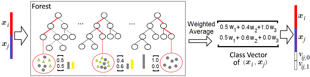
Figure 3: An illustration of the class vector generation taking into account the weights

Now we have numbers $v_{ij,c}^{(k)}$ for every class. Let us analyze these numbers from the point of the SDF aim view.

First, we consider the case when $(\mathbf{x}_{i},\mathbf{x}_{j})\in\mathcal{S}$ and $y_{ij}=0$. However, we may have non-zero $v_{ij,c}^{(k)}$ for both classes. It is obvious that $v_{ij,0}^{(k)}$ (the average probability of class $c=0$) should be as large as possible because $c=y_{ij}=0$. Moreover, $v_{ij,1}^{(k)}$ (the average probability of class $c=1$) should be as small as possible because $c\neq y_{ij}=0$.

We can similarly write conditions for the case when $(\mathbf{x}_{i},\mathbf{x}_{j})\in\mathcal{D}$ and $y_{ij}=1$. In this case, $v_{ij,0}^{(k)}$ should be as small as possible because $c\neq y_{ij}=1$, and $v_{ij,1}^{(k)}$ should be as large as possible because $c=y_{ij}=1$.

In sum, we should increase (decrease) $v_{ij,c}^{(k)}$ if $c=y_{ij}$ ($c\neq y_{ij}$). In other words, we have to find the weights maximizing (minimizing) $v_{ij,c}^{(k)}$ when $c=y_{ij}$ ($c\neq y_{ij}$). The ideal case is when $v_{ij,c}^{(k)}=1$ by $c=y_{ij}$ and $v_{ij,c}^{(k)}=0$ by $c\neq y_{ij}$. However, the vector of weights has to be the same for every class, and it does not depend on a certain class. At first glance, we could find optimal weights for every individual forest separately from other forests. However, we should analyze simultaneously all forests because some vectors of weights may compensate those vectors which cannot efficiently separate $v_{ij,0}^{(k)}$ and $v_{ij,1}^{(k)}$.

6 The SDF training and testing

We apply the greedy algorithm for training the SDF, namely, we train separately every level starting from the first level such that every next level uses results of training at the previous level. The training process at every level consists of two parts. The first part aims to train all trees by applying all pairs of training examples. This part does not significantly differ from the training of the original deep forest proposed by Zhou and Feng [28]. The difference is that we use pairs of concatenated vectors $(\mathbf{x}_{i},\mathbf{x}_{j})$ and two classes corresponding to semantic similarity of the pairs. The second part is to compute the weights $w^{(t,k)}$, $t=1,...,T_{k}$. This can be done by minimizing the following objective function over $M$ unit (probability) simplices in $\mathbb{R}^{T_{k}}$ denoted as $\Delta_{k}$, i.e., over non-negative vectors $\mathbf{w}^{(k)}=(w^{(1,k)},...,w^{(T_{k},k)})\in\Delta_{k}$, $k=1,...,M$, that sum up to one:

$$\min_{\mathbf{w}}J_{q}(\mathbf{w})=\min_{\mathbf{w}}\sum_{i,j}l(\mathbf{x}_{i},\mathbf{x}_{j},y_{ij},\mathbf{w})+\lambda R(\mathbf{w}).$$ (5)

Here $\mathbf{w}$ is a vector produced as the concatenation of vectors $\mathbf{w}^{(k)}$, $k=1,...,M$, $R(\mathbf{w})$ is a regularization term, $\lambda$ is a hyper-parameter which controls the strength of the regularization. We define the regularization term as

$$R(\mathbf{w})=\left\|\mathbf{w}\right\|^{2}.$$

The loss function has to increase values of augmented features $v_{ij,0}^{(k)}$ corresponding to the class $c=0$ and to decrease features $v_{ij,1}^{(k)}$ corresponding to the class $c=1$ for semantically similar pairs $(\mathbf{x}_{i},\mathbf{x}_{j})$. Moreover, the loss function has to increase values of augmented features $v_{ij,1}^{(k)}$ corresponding to the class $c=1$ and to decrease features $v_{ij,0}^{(k)}$ corresponding to the class $c=0$ for dissimilar pairs $(\mathbf{x}_{i},\mathbf{x}_{j})$.

6.1 Convex loss function

Let us denote the set of vectors $\mathbf{w}$ as $\Delta$. In order to efficiently solve the problem (5), the condition of the convexity of $J_{q}(\mathbf{w})$ in the domain of $\mathbf{w}$ should be fulfilled. One of the ways for determining the loss function $l$ is to consider a distance $d(\mathbf{x}_{i},\mathbf{x}_{j})$ between two vectors $\mathbf{x}_{i}$ and $\mathbf{x}_{j}$ at the $q$-th level. However, we do not have separate vectors $\mathbf{x}_{i}$ and $\mathbf{x}_{j}$. We have one vector whose parts correspond to vectors $\mathbf{x}_{i}$ and $\mathbf{x}_{j}$. Therefore, this is a distance between elements of the concatenated vector $\left(\mathbf{x}_{i}^{(-1)},\mathbf{x}_{j}^{(-1)}\right)$ obtained at $q-1$ level and augmented features $\mathbf{v}_{ij}^{(k)}$, $k=1,...,M$, of a special form. Let us consider the expression for the above distance in detail. It consists of $M+1$ terms. The first term denoted as $X_{ij}^{(q)}$ is the Euclidean distance between two parts of the output vector obtained at the previous level

$$X_{ij}=\sum_{l=1}^{m}\left(x_{i,l}^{(-1)}-x_{j,l}^{(-1)}\right)^{2}.$$

Here $x_{i,l}$ is the $l$-th element of $\mathbf{x}_{i}$, $m$ is the length of the input vector for the $q$-th level or the length of the output vector for the level with the number $q-1$.

Let us consider elements $v_{ij,0}^{(k)}$ and $v_{ij,1}^{(k)}$ now. We have to provide the distance between these elements as large as possible taking into account $y_{ij}$. In particular, if $y_{ij}=0$, then we should decrease the difference $v_{ij,1}^{(k)}-v_{ij,0}^{(k)}$. If $y_{ij}=1$, then we should decrease the difference $v_{ij,0}^{(k)}-v_{ij,1}^{(k)}$. Let us introduce the variable $z_{ij}=-1$ if $y_{ij}=0$, and $z_{ij}=1$ if $y_{ij}=1$. Then the following expression characterizing the augmented features $v_{ij,0}^{(k)}$ and $v_{ij,1}^{(k)}$ can be written:

$$\left[\max\left(0,z_{ij}\left(v_{ij,0}^{(k)}-v_{ij,1}^{(k)}\right)\right)\right]^{2}.$$

Substituting (3) into the above expression, we get next $M$ terms

$$\left[\max\left(0,~{}\sum_{t=1}^{T_{k}}P_{ij}^{(t,k)}w^{(t,k)}\right)\right]^{2},\ k=1,...,M,$$

where

$$P_{ij}^{(t,k)}=z_{ij}\left(p_{ij,0}^{(t,k)}-p_{ij,1}^{(t,k)}\right).$$

Finally, we can write

$$d\left(\mathbf{x}_{i},\mathbf{x}_{j}\right)=X_{ij}+\sum_{k=1}^{M}\left[\max\left(0,~{}\sum_{t=1}^{T_{k}}P_{ij}^{(t,k)}w^{(t,k)}\right)\right]^{2}.$$ (6)

So, we have to maximize $d\left(\mathbf{x}_{i},\mathbf{x}_{j}\right)$ with respect to $w^{(t,k)}$ under constraints (4). Since $X_{ij}$ does not depend on $w^{(t,k)}$, then we consider the following objective function

$$J_{q}(\mathbf{w})=\sum_{i,j}\sum_{k=1}^{M}\left[\max\left(0,~{}\sum_{t=1}^{T_{k}}P_{ij}^{(t,k)}w^{(t,k)}\right)\right]^{2}+\lambda\left\|\mathbf{w}\right\|^{2}.$$ (7)

The function $d\left(\mathbf{x}_{i},\mathbf{x}_{j}\right)$ is convex in the interval $[0,1]$ of $w^{(t,k)}$. Then the objective function $J_{q}(\mathbf{w})$ as the sum of the convex functions is convex too with respect to weights.

6.2 Quadratic optimization problem

Let us consider the problem (7) under constraints (4) in detail. Introduce a new variable $\xi_{ij}^{(k)}$ defined as

$$\xi_{ij}^{(k)}=\max\left(0,~{}\sum_{t=1}^{T_{k}}P_{ij}^{(t,k)}w^{(t,k)}\right).$$

Then problem (7) can be rewritten as

$$J_{q}(\mathbf{w})=\min_{\xi_{ij}^{(k)},\mathbf{w}}\sum_{i,j}\sum_{k=1}^{M}\left(\xi_{ij}^{(k)}\right)^{2}+\lambda\left\|\mathbf{w}\right\|^{2},$$ (8)

subject to (4)

$$\xi_{ij}^{(k)}\geq\sum_{t=1}^{T_{k}}P_{ij}^{(t,k)}w^{(t,k)},\ \ \xi_{ij}^{(k)}\geq 0,\ \ (i,j)\in K,\ k=1,...,M.$$ (9)

We have obtained the standard quadratic optimization problem with linear constraints and variables $\xi_{ij}^{(k)}$ and $w^{(t,k)}$. It can be solved by using the well-known standard methods.

It is interesting to note that the optimization problem (8)-(9) can be decomposed into $M$ problems of the form:

$$J_{q}(\mathbf{w}^{(k)})=\min_{\xi_{ij},\mathbf{w}^{(k)}}\sum_{i,j}\xi_{ij}^{2}+\lambda\left\|\mathbf{w}^{(k)}\right\|^{2},$$ (10)

subject to (4)

$$\xi_{ij}\geq\sum_{t=1}^{T_{k}}P_{ij}^{(t,k)}w^{(t,k)},\ \ \xi_{ij}\geq 0,\ \ (i,j)\in K,\ k=1,...,M.$$ (11)

Indeed, by returning to problem (8)-(9), we can see that the subset of variables $\xi_{ij}^{(k)}$ and $w^{(t,k)}$ for a certain $k$ and constraints for these variables do not overlap with the subset of similar variables for another $k$ and the corresponding constraints. This implies that (8) can be rewritten as

$$J_{q}(\mathbf{w})=\sum_{k=1}^{M}\min_{\xi_{ij},\mathbf{w}}\sum_{i,j}\left(\xi_{ij}^{(k)}\right)^{2}+\lambda\left\|\mathbf{w}\right\|^{2},$$

and the problem can be decomposed.

So, we solve the problem (10)-(11) for every $k=1,...,M$ and get $M$ vectors $\mathbf{w}^{(k)}$ which form the vector $\mathbf{w}$. The above means that the optimal weights are separately determined for individual forests.

6.3 A general algorithm for training and the SDF testing

In sum, we can write a general algorithm for training the SDF (see Algorithm 1). Its complexity mainly depends on the number of levels.

Having the trained SDF with computed weights $\mathbf{w}$ for every cascade level, we can make decision about the semantic similarity of a new pair of examples $\mathbf{x}_{a}$ and $\mathbf{x}_{b}$. First, the vectors make to be concatenated. By using the trained decision trees and the weights $\mathbf{w}$ for every level $q$, the pair is augmented at each level. Finally, we get

$$\mathbf{x}_{ab}^{(Q)}=\left(\mathbf{x}_{a}^{(Q)},\mathbf{x}_{b}^{(Q)}\right)=\mathbf{v}_{ab}.$$

Here $\mathbf{v}_{ab}$ is the augmented part of the vector $\mathbf{x}_{ab}^{(Q)}$ consisting of elements from subvectors $\mathbf{v}_{0}$ and $\mathbf{v}_{1}$ corresponding to the class $c=0$ and to the class $c=1$, respectively. The original examples $\mathbf{x}_{a}$ and $\mathbf{x}_{b}$ are semantically similar if the sum of all elements from $\mathbf{v}_{0}$ is larger than the sum of elements from $\mathbf{v}_{1}$, i.e., $\mathbf{v}_{0}\cdot\mathbf{1}^{\mathrm{T}}>\mathbf{v}_{1}\cdot\mathbf{1}^{\mathrm{T}}$, where $\mathbf{1}$ is the unit vector. In contrast to the similar examples, the condition $\mathbf{v}_{0}\cdot\mathbf{1}^{\mathrm{T}}<\mathbf{v}_{1}\cdot\mathbf{1}^{\mathrm{T}}$ means that $\mathbf{x}_{a}$ and $\mathbf{x}_{b}$ are semantically dissimilar and $y_{ab}=1$. We can introduce a threshold $\tau$ for a more robust decision making. The examples $\mathbf{x}_{a}$ and $\mathbf{x}_{b}$ are classified as semantically similar and $y_{ab}=0$ if $\mathbf{v}_{0}\cdot\mathbf{1}^{\mathrm{T}}-\mathbf{v}_{1}\cdot\mathbf{1}^{\mathrm{T}}\geq\tau$. The case $0\leq\mathbf{v}_{0}\cdot\mathbf{1}^{\mathrm{T}}-\mathbf{v}_{1}\cdot\mathbf{1}^{\mathrm{T}}\leq\tau$ can be viewed as undeterminable.

Algorithm 1 A general algorithm for training the SDF

0:  Training set $S$ $=\{(\mathbf{x}_{i},\mathbf{x}_{j},y_{ij}),\ (i,j)\in K\}$ consisting of $N$ pairs; number of cascade levels $Q$

0:  $\mathbf{w}^{(q)}$, $q=1,...,Q$

1:  Concatenate $\mathbf{x}_{i}$ and $\mathbf{x}_{j}$ for all pairs of indices $(i,j)\in K$

2:  Form the training set $R=\{(\mathbf{x}_{i},\mathbf{x}_{j}),y_{ij}),\ (i,j)\in K\}$ consisting of concatenated pairs

3:  for $q=1$, $q\leq Q$  do

4:     Train all trees at the $q$-th level

5:     for $k=1$, $k\leq M_{q}$  do

6:        Compute the weights $\mathbf{w}^{(k)}$ at the $q$-th level from the $k$-th quadratic optimization problem with the objective function (10) and constraints (4) and (11)

7:     end for

8:     Concatenate $\mathbf{w}^{(k)}$, $k=1,...,M$, to get $\mathbf{w}$ at the $q$-th level

9:     For every $\mathbf{x}_{ij}$, compute $\mathbf{v}_{ij}^{(k)}$ at the $q$-th level by using (3), $k=1,...,M$

10:     For every $\mathbf{x}_{ij}$, form the concatenated vector $\mathbf{x}_{ij}$ for the next level by using (2)

11:  end for

It is important to note that the identical weights, i.e., the gcForest can be regarded as a special case of the SDF.

7 Numerical experiments

We compare the SDF with the gcForest whose inputs are concatenated examples from series data sets. In other words, we compare the SDF having computed (trained) weights with the SDF having identical weights. The SDF has the same cascade structure as the standard gcForest described in [28]. Each level (layer) of the cascade structure consists of 2 complete-random tree forests and 2 random forests. Three-fold cross-validation is used for the class vector generation. The number of cascade levels is automatically determined.

A software in Python implementing the gcForest is available at https://github.com/leopiney/deep-forest. We modify this software in order to implement the procedure for computing optimal weights and weighted averages $v_{ij,c}^{(k)}$. Moreover, we use pairs of concatenated examples composed of individual examples as training and testing data.

Every accuracy measure $A$ used in numerical experiments is the proportion of correctly classified cases on a sample of data. To evaluate the average accuracy, we perform a cross-validation with $100$ repetitions, where in each run, we randomly select $N$ training data and $N_{\text{test}}=2N/3$ test data.

First, we compare the SDF with the gcForest by using some public data sets from UCI Machine Learning Repository [17]: the Yeast data set (1484 instances, 8 features, 10 classes), the Ecoli data set (336 instances, 8 features, 8 classes), the Parkinsons data set (197 instances, 23 features, 2 classes), the Ionosphere data set (351 instances, 34 features, 2 classes). A more detailed information about the data sets can be found from, respectively, the data resources. Different values for the regularization hyper-parameter $\lambda$ have been tested, choosing those leading to the best results.

In order to investigate how the number of decision trees impact on the classification accuracy, we study the SDF by different number of trees, namely, we take $T_{k}=T=100$, $400$, $700$, $1000$. It should be noted that Zhou and Feng [28] used $1000$ trees in every forest.

Results of numerical experiments for the Parkinsons data set are shown in Table 2. It contains the accuracy measures obtained for the gcForest (denoted as gcF) and the SDF as functions of the number of trees $T$ in every forest and the number $N=100,500,1000,2000$ of pairs in the training set. It can be seen from Table 2 that the accuracy of the SDF exceeds the same measure of the gcForest in most cases. At that, the difference is rather large for the small amount of training data. In particular, the largest differences between accuracy measures of the SDF and the gcForest are observed by $T=400$, $1000$ and $N=100$. Similar results of numerical experiments for the Ecoli data set are given in Table 3. It is interesting to point out that the number of trees in every forest significantly impacts on the difference between accuracy measures of the SDF and gcForest. It follows from Table 3 that this difference is smallest by the large number of trees and by the large amount of training data. If we look at the last row of Table 3, then we see that the accuracy $0.915$ obtained for the SDF by $T=100$ is reached for the gcForest by $T=1000$. The largest difference between accuracy measures of the SDF and the gcForest is observed by $T=100$ and $N=100$. The same can be seen from Table 2. This implies that the proposed modification of the gcForest allows us to reduce the training time. Table 4 provides accuracy measures for the Yeast data set. We again can see that the proposed SDF outperforms the gcForest for most cases. It is interesting to note from Table 4 that the increasing number of trees in every forest may lead to reduced accuracy measures. If we look at the row of Table 4 corresponding to $N=500$ pairs in the training set, then we can see that the accuracy measures by $100$ trees exceed the same measures by larger numbers of trees. Moreover, the largest difference between accuracy measures of the SDF and the gcForest is observed by $T=1000$ and $N=100$. Numerical results for the Ionosphere data set are represented in Table 5. It follows from Table 5 that the largest difference between accuracy measures of the SDF and the gcForest is observed by $T=1000$ and $N=500$.

The numerical results for all analyzed data sets show that the SDF significantly outperforms the gcForest by small number of training data ($N=100$ or $500$). This is an important property of the SDF which are especially efficient when the amount of training data is rather small.

Table 2: Dependence of the accuracy measures on the number of pairs $N$ and on the number of trees $T$ in every forest for the Parkinsons data set

$T$	$100$		$400$		$700$		$1000$
$N$	gcF	SDF	gcF	SDF	gcF	SDF	gcF	SDF
$100$	$0.530$	$0.545$	$0.440$	$0.610$	$0.552$	$0.575$	$0.440$	$0.550$
$500$	$0.715$	$0.733$	$0.651$	$0.673$	$0.685$	$0.700$	$0.700$	$0.730$
$1000$	$0.761$	$0.763$	$0.778$	$0.786$	$0.803$	$0.804$	$0.773$	$0.790$
$2000$	$0.880$	$0.881$	$0.884$	$0.895$	$0.875$	$0.891$	$0.887$	$0.893$

Table 3: Dependence of the accuracy measures on the number of pairs $N$ and on the number of trees $T$ in every forest for the Ecoli data set

$T$	$100$		$400$		$700$		$1000$
$N$	gcF	SDF	gcF	SDF	gcF	SDF	gcF	SDF
$100$	$0.439$	$0.530$	$0.515$	$0.545$	$0.590$	$0.651$	$0.621$	$0.696$
$500$	$0.838$	$0.847$	$0.814$	$0.823$	$0.836$	$0.845$	$0.821$	$0.837$
$1000$	$0.844$	$0.853$	$0.890$	$0.917$	$0.888$	$0.891$	$0.863$	$0.865$
$2000$	$0.908$	$0.915$	$0.895$	$0.921$	$0.913$	$0.915$	$0.915$	$0.915$

Table 4: Dependence of the accuracy measures on the number of pairs $N$ and on the number of trees $T$ in every forest for the Yeast data set

$T$	$100$		$400$		$700$		$1000$
$N$	gcF	SDF	gcF	SDF	gcF	SDF	gcF	SDF
$100$	$0.454$	$0.500$	$0.484$	$0.511$	$0.469$	$0.515$	$0.469$	$0.575$
$500$	$0.682$	$0.694$	$0.661$	$0.673$	$0.640$	$0.658$	$0.622$	$0.628$
$1000$	$0.708$	$0.711$	$0.713$	$0.723$	$0.684$	$0.710$	$0.735$	$0.737$
$2000$	$0.727$	$0.734$	$0.714$	$0.716$	$0.727$	$0.739$	$0.713$	$0.722$

Table 5: Dependence of the accuracy measures on the number of pairs $N$ and on the number of trees $T$ in every forest for the Ionsphere data set

$T$	$100$		$400$		$700$		$1000$
$N$	gcF	SDF	gcF	SDF	gcF	SDF	gcF	SDF
$100$	$0.515$	$0.515$	$0.535$	$0.555$	$0.530$	$0.555$	$0.535$	$0.540$
$500$	$0.718$	$0.720$	$0.723$	$0.758$	$0.713$	$0.740$	$0.715$	$0.760$
$1000$	$0.820$	$0.830$	$0.837$	$0.840$	$0.840$	$0.860$	$0.885$	$0.895$
$2000$	$0.915$	$0.920$	$0.905$	$0.905$	$0.895$	$0.895$	$0.910$	$0.910$

It should be noted that the multi-grained scanning proposed in [28] was not applied to investigating the above data sets having relatively small numbers of features. The above numerical results have been obtained by using only the forest cascade structure.

When we deal with the large-scale data, the multi-grained scanning scheme should be use. In particular, for analyzing the well-known MNIST data set, we used the same scheme for window sizes as proposed in [28], where feature windows with sizes $\left\lfloor d/16\right\rfloor$, $\left\lfloor d/9\right\rfloor$, $\left\lfloor d/4\right\rfloor$ are chosen for $d$ raw features. We study the SDF by applying the MNIST database which is a commonly used large database of $28\times 28$ pixel handwritten digit images [16]. It has a training set of 60,000 examples, and a test set of 10,000 examples. The digits are size-normalized and centered in a fixed-size image. The data set is available at http://yann.lecun.com/exdb/mnist/. The main problem in using the multi-grained scanning scheme is that pairs of the original examples are concatenated. As a result, the direct scanning leads to scanning windows covering some parts from every example belonging to a concatenated pair, which do not correspond the images themselves. Therefore, we apply the following modification of the multi-grained scanning scheme. Two identical windows simultaneously scan two concatenated images such that pairs of feature windows are produced due to this procedure, which are concatenated for processing by means of the forest cascade. Fig. 4 illustrates the used procedure. Results of numerical experiments for the MNIST data set are shown in Table 6. It can be seen from Table 6 that the largest difference between accuracy measures of the SDF and the gcForest is observed by $T=1000$ and $N=100$. It is interesting to note that the SDF as well as the gcForest provide good results even by the small amount of training data. At that, the SDF outperforms the gcForest in the most cases.

Table 6: Dependence of the accuracy measures on the number of pairs $N$ and on the number of trees $T$ in every forest for the MNIST data set

$T$	$100$		$400$		$700$		$1000$
$N$	gcF	SDF	gcF	SDF	gcF	SDF	gcF	SDF
$100$	$0.470$	$0.490$	$0.520$	$0.520$	$0.570$	$0.585$	$0.530$	$0.570$
$500$	$0.725$	$0.735$	$0.715$	$0.715$	$0.695$	$0.700$	$0.670$	$0.670$
$1000$	$0.757$	$0.770$	$0.755$	$0.760$	$0.775$	$0.780$	$0.830$	$0.840$

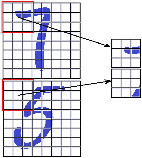
Figure 4: The multi-grained scanning scheme for concatenated examples

An interesting observation has been made during numerical experiments. We have discovered that the variable $z_{ij}$, initially taking the values $-1$ for $y_{ij}=0$ and $1$ for $y_{ij}=1$, can be viewed as a tuning parameter in order to control the number of the cascade levels used in the training process and to improve the classification performance of the SDF. One of the great advantages of the gcForest is its automatic determination of the number of cascade levels. It is shown by Zhou and Feng [28], that the performance of the whole cascade is estimated on validation set after training a current level. The training procedure in the gcForest terminates if there is no significant performance gain. It turns out that the value of $z_{ij}$ significantly impact on the number of cascade levels if to apply the termination procedure implemented in the gcForest. Moreover, we can adaptively change the values of $z_{ij}$ with every level. It has been revealed that one of the best change of $z_{ij}$ is $z_{ij}^{(q)}=2z_{ij}^{(q-1)}$, where $z_{ij}^{(1)}=-1$ for $y_{ij}=0$ and $1$ for $y_{ij}=1$. Of course, this is an empirical observation. However, it can be taken as a direction for further improving the SDF.

8 Conclusion

One of the implementations of the SDF has been represented in the paper. It should be noted that other modifications of the SDF can be obtained. First of all, we can improve the optimization algorithm by applying a more complex loss function and computing optimal weights, for example, by means of the Frank-Wolfe algorithm [9]. We can use a more powerful optimization algorithm, for example, an algorithm proposed by Hazan and Luo [10]. Moreover, we do not need to search for the convex loss function because there are efficient optimization algorithms, for example, a non-convex modification of the Frank-Wolfe algorithm proposed by Reddi et al. [20], which allows us to solve the considered optimization problems. The trees and forests can be also replaced with other classification approaches, for example, with SVMs and boosting algorithms. However, the above modifications can be viewed as directions for further research.

The linear combinations of weights for every forest have been used in the SDF. However, this class of combinations can be extended by considering non-linear functions of weights. Moreover, it turns out that the weights of trees can model various machine learning peculiarities and allow us to solve many machine learning tasks by means of the gsForest. This is also a direction for further research.

It should be noted that the weights have been restricted by constraints of the form (4), i.e., the weights of every forest belong to the unit simplex whose dimensionality is defined by the number of trees in the forest. However, numerical experiments have illustrated that it is useful to reduce the set of weights in some cases. Moreover, this reduction can be carried out adaptively by taking into account the classification error at every level. One of the ways for adaptive reduction of the unit simplex is to apply imprecise statistical models, for example, the linear-vacuous mixture or imprecise $\varepsilon$-contaminated models proposed by Walley [22]. This study is also a direction for further research.

We have considered a weakly supervised learning algorithm when there are no information about the class labels of individual training examples, but we know only semantic similarity of pairs of training data. It is also interesting to extend the proposed ideas on the case of fully supervised algorithms when only the class labels of individual training examples are known. The main goal of fully supervised distance metric learning is to use discriminative information in distance metric learning to keep all the data samples in the same class close and those from different classes separated [18]. Therefore, another direction for further research is to adapt the proposed algorithm for the case of available class labels.

References

- [1] A. Bellet, A. Habrard, and M. Sebban. A survey on metric learning for feature vectors and structured data. arXiv preprint arXiv:1306.6709, 28 Jun 2013.
- [2] S. Berlemont, G. Lefebvre, S. Duffner, and C. Garcia. Siamese neural network based similarity metric for inertial gesture classification and rejection. In Automatic Face and Gesture Recognition (FG), 2015 11th IEEE International Conference and Workshops on, volume 1, pages 1–6. IEEE, May 2015.
- [3] L. Bertinetto, J. Valmadre, J.F. Henriques, A. Vedaldi, and P.H.S. Torr. Fully-convolutional siamese networks for object tracking. arXiv:1606.09549v2, 14 Sep 2016.
- [4] J. Bromley, J.W. Bentz, L. Bottou, I. Guyon, Y. LeCun, C. Moore, E. Sackinger, and R. Shah. Signature verification using a siamese time delay neural network. International Journal of Pattern Recognition and Artificial Intelligence, 7(4):737–744, 1993.
- [5] H. Le Capitaine. Constraint selection in metric learning. arXiv:1612.04853v1, 14 Dec 2016.
- [6] K. Chen and A. Salman. Extracting speaker-specific information with a regularized siamese deep network. In Advances in Neural Information Processing Systems 24 (NIPS 2011), pages 298–306. Curran Associates, Inc., 2011.
- [7] S. Chopra, R. Hadsell, and Y. LeCun. Learning a similarity metric discriminatively, with application to face verification. In 2005 IEEE Computer Society Conference on Computer Vision and Pattern Recognition (CVPR’05), volume 1, pages 539–546. IEEE, 2005.
- [8] Y. Dong, B. Du, and L. Zhang. Target detection based on random forest metric learning. IEEE Journal of Selected Topics in Applied Earth Observations and Remote Sensing, 8(4):1830–1838, 2015.
- [9] M. Frank and P. Wolfe. An algorithm for quadratic programming. Naval Research Logistics Quarterly, 3(1-2):95–110, March 1956.
- [10] E. Hazan and H. Luo. Variance-reduced and projection-free stochastic optimization. In Proceedings of the 33rd International Conference on Machine Learning, volume 48 of ICML’16, pages 1263–1271, 2016.
- [11] J. Hu, J. Lu, and Y.-P. Tan. Discriminative deep metric learning for face verification in the wild. In The IEEE Conference on Computer Vision and Pattern Recognition (CVPR), pages 1875–1882. IEEE, 2014.
- [12] D. Kedem, S. Tyree, K. Weinberger, F. Sha, and G. Lanckriet. Non-linear metric learning. In F. Pereira, C.J.C. Burges, L. Bottou, and K.Q. Weinberger, editors, Advances in Neural Information Processing Systems 25, pages 2582–2590. Curran Associates, Inc., 2012.
- [13] G. Koch, R. Zemel, and R. Salakhutdinov. Siamese neural networks for one-shot image recognition. In Proceedings of the 32nd International Conference on Machine Learning, volume 37, pages 1–8, Lille, France, 2015.
- [14] B. Kulis. Metric learning: A survey. Foundations and Trends in Machine Learning, 5(4):287–364, 2012.
- [15] L. Leal-Taixe, C. Canton-Ferrer, and K. Schindler. Learning by tracking: Siamese cnn for robust target association. arXiv preprint arXiv:1604.07866, 26 Apr 2016.
- [16] Y. LeCun, L. Bottou, Y. Bengio, and P. Haffner. Gradient-based learning applied to document recognition. Proceedings of the IEEE, 86(11):2278–2324, 1998.
- [17] M. Lichman. UCI machine learning repository, 2013.
- [18] Y. Mu and W. Ding. Local discriminative distance metrics and their real world applications. In 2013 IEEE 13th International Conference on Data Mining Workshops (ICDMW), pages 1145–1152. IEEE, Dec 2013.
- [19] M. Norouzi, D. Fleet, and R. Salakhutdinov. Hamming distance metric learning. In P. Bartlett, F.C.N. Pereira, C.J.C. Burges, L. Bottou, and K.Q. Weinberger, editors, Advances in Neural Information Processing Systems 25, pages 1070–1078. Curran Associates, Inc., 2012.
- [20] S.J. Reddi, S. Sra, B. Poczos, and A. Smola. Stochastic frank-wolfe methods for nonconvex optimization. arXiv:1607.08254v2, July 2016.
- [21] N. Srivastava, G. Hinton, A. Krizhevsky, I. Sutskever, and R. Salakhutdinov. Dropout: A simple way to prevent neural networks from overfitting. Journal of Machine Learning Research, 15:1929–1958, 2014.
- [22] P. Walley. Statistical Reasoning with Imprecise Probabilities. Chapman and Hall, London, 1991.
- [23] B. Wang, L. Wang, B. Shuai, Z. Zuo, T. Liu, C.K. Luk, and G. Wang. Joint learning of convolutional neural networks and temporally constrained metrics for tracklet association. In Proceedings of the IEEE Conference on Computer Vision and Pattern Recognition Workshops, pages 1–8. IEEE, 2016.
- [24] D.H. Wolpert. Stacked generalization. Neural networks, 5(2):241–259, 1992.
- [25] C. Xiong, D. Johnson, R. Xu, and J.J. Corso. Random forests for metric learning with implicit pairwise position dependence. arXiv:1201.0610v1, Jan 2012.
- [26] Z. Xu, K.Q. Weinberger, and O. Chapelle. Distance metric learning for kernel machines. arXiv:1208.3422, 2012.
- [27] L. Zheng, S. Duffner, K Idrissi, C. Garcia, and A. Baskurt. Siamese multi-layer perceptrons for dimensionality reduction and face identification. Multimedia Tools and Applications, 75(9):5055–5073, 2016.
- [28] Z.-H. Zhou and J. Feng. Deep forest: Towards an alternative to deep neural networks. arXiv:1702.08835v1, February 2017.