Geometrical optimization approach to isomerization: Models and limitations

Abstract

We study laser-driven isomerization reactions through an excited electronic state using the recently developed Geometrical Optimization procedure [J. Phys. Chem. Lett. 6, 1724 (2015)]. The goal is to analyze whether an initial wave packet in the ground state, with optimized amplitudes and phases, can be used to enhance the yield of the reaction at faster rates, exploring how the geometrical restrictions induced by the symmetry of the system impose limitations in the optimization procedure. As an example we model the isomerization in an oriented 2,2’-dimethyl biphenyl molecule with a simple quartic potential. Using long (picosecond) pulses we find that the isomerization can be achieved driven by a single pulse. The phase of the initial superposition state does not affect the yield. However, using short (femtosecond) pulses, one always needs a pair of pulses to force the reaction. High yields can only be obtained by optimizing both the initial state, and the wave packet prepared in the excited state, implying the well known pump-dump mechanism.

I Introduction

Geometrical Optimization (GeOp) has been recently proposed as a method to engineer the initial state within a manifold of allowed or accessable initial levels in order to maximize the yield of population transfer to a single state or a set of states belonging to another manifold of levelspar1 ; par2 . The method has led to the discovery of Parallel Transfer (PT) as a mechanism of efficient electronic absorption with strong and short (e.g. femtosecond) laser pulsespar1 ; par3 . PT accelerates the desired transition using weaker fields and can be used to achieve selective excitation with pulses with bandwidths much larger than the vibrational spacing. It has been argued that there are geometrical (or structural) aspects of the Hamiltonian underlying the success of the PT processpar3 . In this work we investigate their role in the control of isomerization reactions, where the geometry of the problem has a clear direct impact on the process under study.

Quantum control has been used with great success to significantly enhance the yields of photodissociation reactions by precise tailoring of laser pulsesQC1 ; QC2 ; QC3 ; QC4 . Many different strategies have been suggested contributing to knowledge on key aspects of the quantum dynamics, particularly under strong fieldsSS1 ; SS2 . Experiments typically use pulse-shaping technologiesshaping1 ; shaping2 and learning algorithmsLA have been used in a wide variety of systemsPDexp1 ; PDexp2 ; PDexp3 ; PDexp4 ; PDexp5 ; PDexp6; PDexp7 .

Numerical results using N-level Hamiltonians under long pulses and wave-packet calculations in reduced ($1$ or $2$)-dimensional models for short pulse dynamics have also shown great promise in the possibility of driving isomerization reactions pipulse1 ; pipulse2 ; pipulse3 ; spulse1 ; spulse2 ; spulse3 ; spulse4 ; spulse5 ; chirp2 ; STIRAP1 ; STIRAP2 ; STIRAP3 ; STIRAP4 and even distinguishing optical isomers or purifying a racemate mixturepipulse4 ; chirp1 ; CPL1 ; CPL2 ; CPL3 ; CPL4 ; CPL5 ; BS1 ; BS2 ; BS3 ; BS4 ; BS5 ; VE . The most general models of population transfer were applied. For instance, population inversion via $\pi$ pulses were used with sequences of IR pulsespipulse1 ; pipulse2 ; pipulse3 ; pipulse4 or a single short IR pulse, acting in a pump-dump mechanismspulse1 ; spulse2 ; spulse3 ; spulse4 . Despite using relatively simple models, much attention was devoted to analyzing the robustness of the schemes to different types of intra- or inter-molecular couplingsrobustness ; spulse2 . Adiabatic passage using chirped pulseschirp1 ; chirp2 , STIRAPgSTIRAP1 (Stimulated Raman adiabatic passage) STIRAP1 ; STIRAP2 ; STIRAP3 ; STIRAP4 or even half-STIRAPchirp1 , were also used.

The same approaches were also applied to the more difficult case of symmetric isomerization reactions, as in optical isomers. Here the polarization plays an important roleCPL1 ; CPL2 ; CPL3 ; CPL4 ; CPL5 , but the linear components of the polarized field can work separately if there operates a mechanism for breaking the parity of the systemBS1 ; BS2 ; BS3 ; BS4 ; BS5 or in the simpler scenario where the molecule is aligned with the electric fieldpipulse4 ; chirp1 . Even recent approaches with strong fields, based on the role of Stark effects strong1 ; strong2 ; strong3 ; strong4 or the use of counterdiabatic pulses to accelerate adiabatic passagecounter were proposed and tested.

Despite the many suggested control mechanisms, there is still limited success in controlling isomerization reactions in experiments. The experiments work with strong fields and use the excited electronic state as an intermediate of the reactionexp1 ; exp2 ; exp3 ; exp4 ; exp5 ; exp6 ; exp7 . The reason is not only due to technological limitations in the set of IR sources available (and the difficulties in modulating these pulses), but it is also motivated by important physical reasons. In the Franck-Condon region of the excited state, the initial wave function experiences a natural force towards the reaction coordinate, that can in principle lead to fast isomerization in the absence of an internal barrier. In addition, because of intramolecular vibrational redistribution (IVR) in and conical intersections of excited states (or other non-adiabatic couplings) one typically needs to move the population rapidly through the transition state, which favors doing it in the absence of a barrier in the excited state. Using strong fields to drive the electronic absorption leads naturally to study the effect of vibrational motion (or vibrational coherence) to enhance such absorptionIRUV1 ; IRUV2 ; IRUV3 ; IRUV4 ; IRUV5 ; IRUV6 ; IRUV7 ; IRUV8 ; IRUV9 . Recent results in two-photon processes (such as a pump-dump mechanism) have shown that the optimization of the initial wave packet is less important when the pulses are time-delayedGeOp2photon . In this work we investigate its role in isomerization reactions, with the wider goal of finding new mechanisms to enhance the yield and especially accelerate the rate of the reaction. To that end we study the cis-trans isomerization in 2,2’-dimethyl-biphenyl. In Sec.2 we explain the model and summarize how we apply the GeOp algorithm to the two-photon process. In Sec.3 we show the numerical results and build a simple analytical model to explain the main observations. Sec.4 is the conclusions.

II Models and Methods

As a simple general model for isomerization reactions, we use quartic symmetric one-dimensional potentials with parameters fitted using spectroscopic data to obtain potentials for the ground ($V_{g}(x)$) and first excited electronic state ($V_{e}(x)$), respectively. In this work we analyze the dynamics only in the reaction coordinate. Then we obtain the Hamiltonian in the energy representation, applying the Fourier Grid Hamiltonian (FGH)FGH . The transition dipole matrix elements are evaluated assuming the Condon limit. Since we want to stress some geometrical features of the solution, we use as a representative example the torsion of the phenyl groups in the isomerization of the 2,2’-dimethyl-biphenyl, which we represent by a double well potential.

II.1 Parameters of the isomerization in 2,2’-dimethyl-biphenyl

Although to model torsional potentials one often uses polynomials of trigonometric functions ($\cos(m\theta)$) of the torsional angle $\theta$, we, for simplicity, model the dimethyl-biphenyl ground state using a quartic expression. This is also justified because the control schemes that we use are properly described in the energy representation, so that we are mainly interested in having a model as general as possible that approximately reproduces the energetics of the isomerization reaction. In that regard we will use scaled units. Writing

$$V_{g}(x)=\frac{1}{2}\beta x^{2}\left[\frac{x^{2}}{2x_{0}^{2}}-1\right]$$ (1)

where $x$ is a generalized reaction coordinate, such that $2x_{0}$ is the separation between the equilibrium configurations of both isomers (approximately the torsional angle displacement between the isomers, here $90.7^{\circ}$Grein ), and $\beta$ plays the role of the spring constant of the oscillator in each equilibrium configuration. Hence, the fundamental frequency of the torsional motion is obtained from $\beta=m\omega_{0}^{2}/2$, where $m$ is the moment of inertia and its value is fixed as $m=1$. In the transition state ($x=0$), the potential is zero. The torsional energy barrier separating the isomers is calculated as $E_{b}=V_{g}(0)-V_{g}(\pm x_{0})=m\omega_{0}^{2}x_{0}^{2}/8$. In this work the energies are scaled with respect to $\omega_{0}$, so we use $\beta=1/2$. Calculations at the level of density functional theory estimated a isomerization barrier of $16.7$ Kcal/molGrein ($5841$ cm^-1), which is much larger than that in the unsubstituted biphenyl molecule ($E_{b}\sim 500$ cm^-1Takei ). In the biphenyl substituted with methyl groups there will be many more states belonging to the reactant and product, making it an excellent example of the capabilities of the parallel transfer control mechanismpar1 ; par2 .

For the fundamental frequency of the torsional motion, $\omega_{0}$, we use data from biphenyl, where $\omega_{0}=70$ cm^-1Takei , and apply a mass correction due to the different reduced masses of the rings in the dimethyl biphenyl $\mu_{d}$ and the biphenyl molecule $\mu_{0}$, $\mu_{d}/\mu_{0}=1.195$. Hence, we assume for the 2,2’-dimethyl biphenyl $\omega_{0}\approx 64$ cm^-1, and thus $E_{b}/\omega_{0}\sim 91.3$ and $x_{0}=27$.

There is relatively few detailed information concerning the excited electronic states of the dimethyl biphenyl molecule, but the peak of the $B$ band ($\lambda_{\mathrm{max}}\sim 227$ nmSuzuki ) is not very displaced from that in biphenyl ($\lambda_{\mathrm{max}}\sim 237.5$ nmbiphenyl1 ; biphenyl2 ; biphenyl3 ), although the peak intensity is smaller. In biphenyl, the excited state has a minimum near $\theta=0$ and the potential is very flat around the equilibrium geometrybiphenyl1 ; biphenyl2 ; biphenyl3 . We model the excited state in the 2,2’-dimethyl biphenyl potential as a barrierless quartic potential

$$V_{e}(x)=\alpha x^{4},$$ (2)

with $\alpha=2\cdot 10^{-4}$. The energy gap between the electronic states is included in the frequency of the pulse.

To construct the Hamiltonian matrix we use the first $100$ localized eigenstates of the ground potential ($50$ belonging to each isomer) and $121$ levels in the excited potential (those with quantum numbers from $v^{\prime}=180$ to $v^{\prime}=300$) and apply the FGH procedure.

II.2 Geometrical Optimization

In the ground electronic state, the system has a set of (localized) vibrational states that belong to isomer A, $|A,j\rangle$, and a set of (localized) vibrational states that belong to isomer B, $|B,k\rangle$. We are only interested in stable isomers. In addition, there will be (delocalized) vibrational states with energy larger than the internal isomerization barrier. These states will not be used in the geometrical optimization procedure. The reaction will proceed through the excited electronic state E with delocalized vibrational states $|E,l\rangle$. We are interested in maximizing the overall yield of the isomerization reaction, defined as

$$\chi_{i}=\sum_{k\in B}\left|\langle B,k|{\sf U}(T,0;\epsilon_{p},\epsilon_{S})|\psi^{A}_{i}\rangle\right|^{2}$$ (3)

where the initial state $|\psi^{A}_{i}\rangle=\sum_{j}^{N_{c}}a_{ji}|A,j\rangle$ is a superposition state involving $N_{c}$ vibrational levels of the initial isomer. We sum over all the vibrational levels that belong to $B$ (that is, the localized states, abbreviated as $k\in B$) at final time, $T$. The propagator ${\sf U}(T,0;\epsilon_{p},\epsilon_{S})$ depends on two external fields, the pump pulse $\epsilon_{p}(t)$ and the dump (or Stokes) pulse $\epsilon_{S}(t)$. For the derivation of the more general equations, we assume that each field drives a different transition, although for the 2,2’-dimethyl-biphenyl or any other symmetrical system, both pulses couple each isomer to the excited state. Then the propagators will depend on a field $\epsilon_{0}(t)=\epsilon_{p}(t)+\epsilon_{S}(t)$. In general we will omit the-time dependence for brevity. For each superposition state $|\psi^{A}_{i}\rangle$ one obtains a different yield, $\chi_{i}$.

We want to find $|\psi^{A}_{i}\rangle$ that maximizes $\chi_{i}$ for a given set of pulses $\epsilon_{p}$, $\epsilon_{S}$. If we are only allowed to change the initial state, the amplitudes of the superposition can be obtained using a variational method. The result gives the matrix equationpar2

$$\sum_{k\in B}^{N_{c}}\left(F_{jk}-\chi_{i}\delta_{jk}\right)a_{ki}=0$$ (4)

where $\delta_{jk}$ is the Kronecker delta and the operator ${\sf F}$ has matrix elements

$$\begin{array}[]{cl}F_{jk}=\sum_{n\in N_{B}}&\langle A,j|{\sf U}^{\dagger}(T,0;\epsilon_{p},\epsilon_{S})|B,n\rangle\\ &\times\langle B,n|{\sf U}(T,0;\epsilon_{p},\epsilon_{S})|A,k\rangle\end{array}$$ (5)

However, if the time-evolution is split in different time-intervals, it is possible to geometrically optimize the wave function in between. This is most natural when the optimization is performed over a well defined set of states. For instance, in the isomerization reaction, if the pump- and Stokes-pulses are time-delayed, it is natural to ask how the yield of the reaction can be improved if the wave function in the excited state can be prepared after $\epsilon_{p}$ and before $\epsilon_{S}$ acts.

We first rewrite in detail the sum over the excited states $|E,l\rangle$ in the yield

$$\chi_{i}=\sum_{k\in B}\left|\sum_{l\in E}\langle\psi^{A}_{i}|{\sf U}_{1}^{\dagger}(T_{m},0;\epsilon_{p})|E,l\rangle\right.$$

$$\left.\langle E,l|{\sf U}_{2}^{\dagger}(T,T_{m};\epsilon_{S})|B,k\rangle\right|^{2},$$ (6)

where $T_{m}$ is the time at which $\epsilon_{p}(t)$ is switched off and the indices $1$ and $2$ refer to the propagators that depend on the first and second pulses, respectively. Then we allow ourselves to change the intermediate state before $\epsilon_{S}$, by which we start the stimulated emission in the so-called “bridge state” $|\psi_{b}^{E}\rangle$, instead of the state prepared after $\epsilon_{p}$, $|\psi^{E}(T_{m})\rangle$. We now rename $\chi_{ib}$ to the isomerization yield, as it depends on two wave functions, $|\psi^{A}_{i}\rangle$ and $|\psi^{E}_{b}\rangle$, and rewrite the equation as

$$\chi_{ib}=\sum_{l\in E}\left|\langle\psi^{A}_{i}|{\sf U}_{1}^{\dagger}(T_{m},0;\epsilon_{p})|E,l\rangle\right|^{2}\times$$

$$\sum_{k\in B}\left|\langle\psi^{E}_{b}|{\sf U}_{1}^{\dagger}(T_{m},0;\epsilon_{p})|B,k\rangle\right|^{2}=\chi_{i}\chi_{b}$$ (7)

which is a product of the yields for each one-photon process. More restrictive optimization procedures are also possibleNote .

By the geometrical optimization procedure we can maximize the yield with respect to $|\psi^{A}_{i}\rangle$ and $|\psi^{E}_{b}\rangle$, the latter being a superpositon of $N_{E}$ vibrational levels of the $E$ state, $|\psi^{E}_{b}\rangle=\sum_{l\in N_{E}}e_{lb}|E,l\rangle$. It is important to notice that the optimization of $|\psi^{E}_{b}\rangle$ requires some preparation time $T_{p}$ that is included in ${\sf U}_{2}(T,T_{m};\epsilon_{S})$. Because we use the GeOp procedure and therefore we do not treat the process dynamically, $T_{p}$ is not defined. Hence, the time-delay between the pump and Stokes is not defined either.

We obtain $|\psi^{E}_{b}\rangle$ by maximizing the one-photon transition from the $E$ to the $B$ state via ${\sf U}_{2}(T_{m},T;\epsilon_{S})$, yielding the eigenvalue equation

$$\sum_{k\in E}^{N_{E}}\left(G_{jk}-\chi_{b}\delta_{jk}\right)e_{kb}=0$$ (8)

where

$$G_{jk}=\sum_{k\in B}\langle E,j|{\sf U}^{\dagger}_{2}(T,T_{m};\epsilon_{S})|B,k\rangle\langle B,k|{\sf U}_{2}(T,T_{m};\epsilon_{S})|E,k\rangle$$ (9)

On the other hand, the initial state $|\psi_{i}^{A}\rangle$ is found by maximizing the transition probability from $A$ to $E$ conditioned on the choice of $\epsilon_{p}$. It must satisfy the equation

$$\sum_{k\in A}^{N_{A}}\left(F_{jk}-\chi_{i}\delta_{jk}\right)a_{ji}=0$$ (10)

where

$$F_{jk}=\sum_{k\in N_{E}}\langle A,j|{\sf U}^{\dagger}_{1}(T_{m},0;\epsilon_{p})|E,k\rangle\\ \langle E,k|{\sf U}_{1}(T_{m},0;\epsilon_{p})|A,i\rangle$$

Finally, the yield for the isomerization reaction is obtained as $\chi_{ib}=\chi_{i}\chi_{b}$. Unless otherwise speficied, we always choose the number of levels that participate in each of the optimizations, such that they span the same energy bandwith, e.g. if $n_{i}$ and $n_{f}$ and $m_{i}$ and $m_{f}$ are the smaller/larger quanta within $N_{A}$ and $N_{E}$ respectively, we constrain the levels that we choose in both maximizations so that their energy differences are equal, $E(n_{f})-E(n_{i})=E(m_{f})-E(m_{i})$.

In the case of 2,2’-dimethyl-biphenyl the previous equations remain valid by simply changing $\epsilon_{p}$ and $\epsilon_{S}$ by $\epsilon_{0}$ which is the sum of both. Now ${\sf U}_{1}$ and ${\sf U}_{2}$ are the same propagators. However, $G_{jk}$ and $F_{jk}$ are not equal because of the different role of the initial and final states in Eqs.(7) and (9). In addition, in this case it is possible to use a single long pulse $\epsilon_{0}(t)$ that could drive both the pump and dump processes.

III Controlling the dimethyl-biphenyl isomerization

III.1 Numerical Results

We integrate the time-dependent Schrödinger equation (TDSE) in the energy representation for the $1D$-model Hamiltonian with different parameters of the pulses (peak amplitude and duration). We use Gaussian pulses and the pulse frequencies are chosen to resonantly excite an excited state $|E,k\rangle$ ($k=220$) that maximizes the Franck-Condon factor with the ground state level, $|\langle E,k|A,0\rangle|^{2}$. The dipole matrix element $\langle E,220|A,0\rangle=0.109$, while $\langle E,220|B,0\rangle=-0.109$ (the sign depends on the numerical procedure since the symmetrized states are degenerate).

The reaction yield (final population in $B$) is represented as a function of the pulse areaShore (omitting the factor $ea_{0}/\hbar$)

$${A_{0}}=\int_{-\infty}^{\infty}\epsilon_{0}(t)dt$$ (11)

which parametrizes the integrated strength of the coupling, as discussed in detail in the following section. Hence, when comparing results obtained with pulses of different duration at a given $A_{0}$ one must take into account that the actual amplitudes differ. Since the energy of the pulse depends on the intensity and duration, the results obtained using shorter pulses (at a fixed $A_{0}$) imply using stronger pulses.

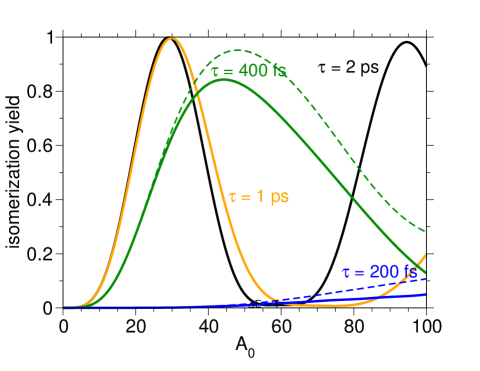
Figure 1: Yield of isomerization as a function of the pulse area $A_{0}$ of the single long pulse that drives the reaction, for different pulse durations (solid lines). Also shown are results obtained when the initial wave function is a superposition state optimized to maximize the transfer (dashed lines). Using long pulses the yield can barely improve since essentially one one quantum pathway links the same initial and final states, and therefore there is no interference.

First, we study the effect of pulses of duration (full width half maximum, fwhm) $\tau=200$ fs, $400$ fs, $1$ and $2$ ps starting in $|A,0\rangle$. The isomerization reaction is driven by a single pulse, which is possible since both isomers have the same energy. In Fig. 1 we show the yield of isomerization at the end of the pulse starting in the ground vibrational level. Since the energy spacing between adjacent levels is $64$ cm^-1 in the ground state (smaller in the excited state), using $1$ or $2$ ps pulses the states are energy-resolved and the system behaves mainly as a $3$-level system in so-called $\Lambda$ configuration. That is, basically only $3$ levels participate and the dynamics show some kind of Rabi oscillations. As discussed in the following section [Sec.III.b] the oscillations follow a sine to the fourth behavior, which is characteristic of two-photon (or pump-dump) processes.

However, with shorter pulses ($\tau=400$ fs) one first observes deviations at larger intensities that produce asymmetries in the Rabi oscillation. For even shorter pulses the population transfer to the isomer $B$ is basically blocked. Using strong fields ($A_{0}\sim 30$) one observes first substantial population in the excited intermediate state ($\sim 70$%) and then Raman excitation.

It is known that, using longer pulses, the optimization of the initial state does not improve the results beyond the possible benefit of exploiting larger transition-dipole matrix-elements, since there are no possible interfering pathwayspar3 . We have applied the GeOp procedure to the dynamics driven by the shorter pulses, optimizing the initial wave function as a superposition of the $2$ or $4$ lowest vibrational levels for the $\tau=400$ and $\tau=200$ fs pulses, respectively. The results with even shorter pulses ($\tau\leq 40$ fs) show yields smaller than $0.005$ even considering GeOp with a large number ($10-20$) of vibrational levels, hence they are not shown in the figure. Clearly, the isomerization reaction cannot be driven efficiently by a single ultrashort pulse.

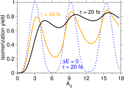
Figure 2: Yield of isomerization as a function of the pulse area $A_{0}$ with pulses of different durations for a pump and dump process (using two identical time-delayed pulses) where both the initial state and the intermediate state are optimized to maximize the yield of each respective optical transition. The dotted line represents the results where we model the system with degenerate vibrational levels, as explained in the text.

In order to drive the isomerization reaction more effectively with shorter pulses we must split the driving pulse in two, and optimize both the initial $|\psi^{A}_{i}\rangle$ and the intermediate state $|\psi^{E}_{b}\rangle$. Since the excited state is optimized, $|\psi^{E}_{b}\rangle$ is not necessarily dynamically connected to the state prepared after the pump pulse, $|\psi^{E}(T_{m})\rangle=U_{1}(T_{m},0;\epsilon_{1})|\psi^{A}_{i}\rangle$.

In Fig. 2 we show the results of the optimization using pulses of $40$ and $20$ fs durations (fwhm) and different pulse amplitudes, parametrized as a function of the pulse area [Eq.(10)]. For the results with $40$ fs pulses we use the lowest $13$ vibrational levels in $A$ to optimize $|\psi^{A}_{i}\rangle$ and $20$ levels in $E$ around $v=220$, such that approximately both sets of levels span the same bandwidth, which is approximately the pulse bandwidth. For the optimization with $20$ fs pulses we use $25$ levels in $A$ and $37$ in B. Using the same conditions, we also show the results that would be obtained using a simplified model Hamiltonian where we keep the same couplings, but make all states degenerate. In this model one can obtain insightful analytical resultspar3 .

The yield of isomerization shows oscillations. Comparing these oscillations with those obtained using a single long pulse, we observe that with two pulses (optimizing the $|\psi^{E}_{b}\rangle$ state) one can achieve high yields at significantly lower pulse areas. This is a feature of parallel transfer, where absorption (or stimulated emission) can be accelerated by maximizing the use of the effective transition dipole between the electronic states. The required area can roughly decrease with the number of levels that participate. On the other hand, the results are relatively similar for the $20$ and $40$ fs pulses, although the maximum yields can be slightly larger (but more sensitive to the area) for the shorter pulse. This reflects some results obtained in one-photon processes, where the parallel transfer depends more crucially on the initial phases for shorter pulses, imposing some kind of generalized pulse area theorempar2 . For longer pulses dynamical phases become more important. The maximum yields are smaller but the sensitivity to the area decreases. In the opposite extreme, by removing the dynamical phases (imposing degenerate states in the Hamiltonian) one reproduces perfect Rabi oscillations, characteristic of a simple $3$-level system. We explain the process in more detail in the following section.

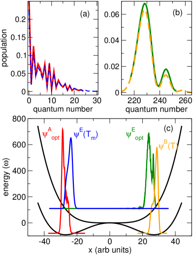
Figure 3: In (a) we compare the optimal initial wave packet $|\psi^{A}_{\mathrm{opt}}\rangle$ (orange line) with the final state prepared after the dump pulse in the B isomer $|\psi^{B}(T)\rangle$ (black dashed line) in the energy representation (vibrational quantum numbers). In (b) we compare the optimal bridge state $|\psi^{E}_{\mathrm{opt}}\rangle$ (orange line) with the wave packet prepared after the pump pulse (black dashed line). In (c) we show the different wave packets in the position representation. See the text for more information.

To understand the results of the optimization procedure we need to consider the geometrical mechanism behind the process. In Fig. 3 we compare the state that is prepared after the first pulse (at time $T_{m}$), $|\psi^{E}(T_{m})\rangle$, with the optimized intermediate state $|\psi^{E}_{\mathrm{opt}}\rangle$. Because we limit the number of states that can participate in the superposition, the populations in $|\psi^{E}_{\mathrm{opt}}\rangle$ are rescaled with respect to those in $|\psi^{E}(T_{m})\rangle$, but otherwise are similar. The effect of the optimization is basically to change the relative phases of the wave packet components. The effect can be visualized in the coordinate representation as a displacement of the wave packet from near the Franck-Condon region of the $E\leftarrow A$ transition, to near the Franck-Condon region of the $B\leftarrow E$ transition. The optimization in the intermediate state is essentially equivalent to adding a time-delay that allows the wave packet prepared at time $T_{m}$ to move from one region of the potential to another, plus additional corrections that minimize the wave packet spreading that would occur in free evolution.

The same analysis can be performed on $|\psi^{A}_{\mathrm{opt}}\rangle$ and the final wave function that is prepared in the $B$ isomer, $|\psi^{B}(T)\rangle$. Because the system is very symmetrical, both states are also very similar, showing the validity of the analytical solutions and the underlying geometrical features that govern the GeOp procedure.

In Fig.3(c) we reconstruct the wave functions in the generalized coordinate $x$, $|\langle x|\psi\rangle|^{2}$, from the amplitudes and the eigenstates obtained using the FGH method. As indicated, the optimization amounts to a displacement of the excited wave function. Although the parallel transfer increases the rate of absorption from $A$ to $E$ and stimulated emission from $E$ to $B$, because the limiting factor is given by the free evolution in the intermediate state (or alternatively the preparation of the optimal intermediate state) there is little gain in the overall rate of the isomerization.

III.2 Simple analytical models

In the long-pulse, weak-interaction regime, as in the results of Fig. 1 (particularly for $\tau=1$ ps) the $1D$ molecular model can be approximated by a simple $3$-level system, where the initial and final states are both coupled by the same field $\epsilon_{0}(t)$ with the intermediate excited state. Under these conditions the TDSE equation can be integrated analytically in the rotating wave approximation (RWA), where only the in-phase component of the periodic oscillation of the laser $\cos(\omega t)\approx\exp(\pm i\omega t)/2$, is kept (the negative part in the absorption and the positive in the stimulated emission). The final population in $|B,0\rangle$ (which is equal to the yield of isomerization in this model) is

$$\chi=|\langle B,0|\psi(\infty)\rangle|^{2}=\sin^{4}\left(\mu{A_{0}}/\sqrt{8}\right)$$ (12)

where $\mu$ is the absolute value of the transition dipole between the states, $\mu\sim 0.109$. This result implies a minimum pulse area of $A_{0}=\sqrt{2}\pi/\mu$ in order to reach the maximum yield of isomerization.

For comparison, if both transitions were independent, the reaction could proceed sequentially, first from $|A,0\rangle$ to the intermediate state and then from the intermediate state to $|B,0\rangle$. The simple two level system implies population transfer that depends as $\sin^{2}(A_{0}/2)$ (the Rabi formula) given a minimum pulse area of $\pi$ for each transition, and a total area of $2\pi$ for the two pulses to drive the isomerization reaction.

To understand the results using shorter pulses we must address several questions. The first one is why the isomerization reaction cannot be driven by a single (ultrashort) pulse. The second one is how the absorption and stimulated emission processes can be accelerated, that is, how the Rabi oscillations of the yield depend on the number of levels in the superposition. In the context of the model in the energy-representation, the first question can be seen to depend on some features of the signs of the Franck-Condon factors, some of which are related to the symmetry of the system. The second is a general feature of parallel transfer.

For the optical isomer one can find fundamental symmetry rules based on the symmetrized eigenfunctions. The excited states, $|E,j\rangle$, are symmetric or antisymmetric with respect to parity for even and odd values of $j$, respectively. For the ground electronic potential, one can create states with well defined symmetry: $|+,j\rangle=\left(|A,j\rangle+|B,j\rangle\right)/\sqrt{2}$ and $|-,j\rangle=\left(|A,j\rangle-|B,j\rangle\right)/\sqrt{2}$.

To uniquely correlate the sign with the parity for all possible values of $j$, the wave function in $B$ must flip its sign for even $j$. Because the signs of wave functions are arbitrary this global gauge fixing is allowed. The matrix elements are different depending on the choice of phases, but the final results of the dynamics do not change. Here we adopt this choice to simplify the analysis. Then some general properties of the matrix elements can be easily calculated. For symmetric transition dipoles (as in the Condon limit), $\langle E,k|\mu|+,j\rangle=[1+(-1)^{k}]/2$ and $\langle E,k|\mu|-,j\rangle=[-1+(-1)^{k}]/2$. Writing $|A,j\rangle$ and $|B,j\rangle$ in terms of $|+,j\rangle$ and $|-,j\rangle$, $|A,j\rangle=\left(|+,j\rangle+|-,j\rangle\right)/\sqrt{2}$, $|B,j\rangle=\left(|+,j\rangle-|-,j\rangle\right)/\sqrt{2}$, one can obtain the fundamental symmetry rule for the nondiagonal Hamiltonian elements in terms of the localized states,

$$\langle E,k|\mu|A,j\rangle=(-1)^{k}\langle E,k|\mu|B,j\rangle$$ (13)

which implies that the sign of the matrix elements only depends on the parity of the $|E,k\rangle$ states. For antisymmetric transition dipoles one must multiply the second term by $(-1)^{k+1}$.

Now assume, for simplicity, that the dipole matrix elements have equal magnitude and only differ in sign, which only depends on the vibrational level $|E,k\rangle$, $\langle E,k|\mu|A,i\rangle=\mathrm{sign}_{1}(k)\mu$, $\langle E,k|\mu|B,j\rangle=\mathrm{sign}_{2}(k)\mu$ (alternatively consider first that there is only one active vibrational level in $A$ and $B$) and that all levels are degenerate, as in the model tested in Sec.3A. Then starting in $|A,0\rangle$, the pulse prepares a superposition state $|\psi^{E}(T_{m})\rangle=\sum_{k}\mathrm{sign}_{1}(k)|E,k\rangle/\sqrt{N_{E}}$ (where $N_{E}$ is the number of accessible levels in the excited state). The amplitude in this superposition will depend on the pulse parameters, but all the population in the excited state will be in $|\psi^{E}\rangle$, as

$$\langle\psi^{E}(T_{m})|\mu|A,i\rangle=\mu\sum_{k}\mathrm{sign}_{1}(k)^{2}/\sqrt{N_{E}}=\sqrt{N_{E}}\mu$$

is the only non zero matrix element of the Hamiltonian, or alternatively, $|\psi^{E}\rangle$ is the only bright state.

In addition, in the absence of dynamical phases, the superposition does not change. Its coupling with any vibrational level in the $B$ isomer is $\langle B,j|\mu|\psi^{E}(T_{m})\rangle=\mu^{2}\sum_{k}\mathrm{sign}_{2}(k)\mathrm{sign}_{1}(k)=\mu^{2}\sum_{k}(-1)^{k}=0$. Hence a single ultrafast pulse cannot move the population directly from the $A$ isomer to the $B$. This will occur whenever there are at least two $k$ levels involved in the sum (it does not restrict population transfer using long pulses). The dynamical phases, however, can change the sign of the superposition such that it is no longer orthogonal to the $|B,j\rangle$ levels. But this change depends on the mass of the system and induces, in the coordinate representation, the motion of the wave packet $|\psi^{E}(t)\rangle$.

On the other hand, in order to accelerate the transition from $A$ to $E$ and to avoid the Raman decoupling (Autler-Townes splitting) induced by the initially unpopulated vibrational levels in $A$, one just needs to prepare an initial superposition state in the form $|\psi^{A}_{i}\rangle=\sum_{j}|A,j\rangle/\sqrt{N_{A}}$, where $N_{A}$ is the number of accessible levels in $A$. This state will also prepare $|\psi^{E}(T_{m})\rangle$ but the coupling

$$\langle\psi^{E}(T_{m})|\mu|\psi^{A}_{i}\rangle=\mu\sum_{j}\sum_{k}\mathrm{sign}_{1}(k)^{2}/\sqrt{N_{A}N_{E}}=$$

$=\sqrt{N_{A}N_{E}}\mu$, increases with the number of participating levels in the superposition. The same argument applies to optimize $|\psi^{E}_{b}\rangle$ in order to accelerate the transition to $B$. However, as discussed, $\langle\psi^{E}_{b}|\psi^{E}(T_{m})\rangle=0$.

Although for enantiomers this orthogonality is enforced by symmetry, reflected in the signs of the dipole matrix elements, the negligible overlap of the excited state prepared in the Franck-Condon region of the $A$ isomer with respect to the $B$ states is a rather general geometrical principle that stems from the fact that both equilibrium configurations are spatially separated. As the results in Fig. 3 show, the geometrical optimization can find the superposition states that accelerate the absorption from isomer $A$ to the excited state and the stimulated emission from $E$ to isomer $B$. These wave functions sit in their respective Franck-Condon regions and do not overlap. Hence it is not possible to accelerate the whole isomerization reaction. The optimization of $|\psi^{E}_{b}\rangle$ on the other hand, basically amounts to waiting for the wave packet prepared in $E$ after the first pulse ends $|\psi^{E}(T_{m})\rangle$ to reach, by free evolution in $B$, to the other Franck-Condon window. This process is limited by the dynamical phases (mass of the system) and cannot be accelerated. In short, what the GeOp scheme discovers is the well-known pump-dump process.

IV Conclusions

We have studied the laser-driven isomerization reaction of an oriented 2,2’-dimethyl biphenyl molecule through an excited barrierless electronic state using the recently developed Geometrical Optimization procedure. Our goal was to analyze whether an initial wave packet in the ground state, with optimized amplitudes and phases, could be used to enhance the yield of the reaction at faster rates, exploring how the geometrical restrictions induced by the symmetry of the system impose limitations in the optimization procedure. We used a very simple general $1$-D model for the system, based on symmetric quartic potentials. The study omits further interesting considerations involving the neglected dimensions of the system, and hence, possible competing processes such as IVR or intersystem crossing at conical intersections, which will likely play a role in a more realistic model of the dynamics, even using short pulses.

We have found that using long (picosecond) pulses the reaction can be driven by a single pulse and the results are not sensitive to the initial state coherences. Hence, the geometrical optimization procedure is not necessary in this limit as no PT is possible.

On the other hand, using shorter (femtosecond) pulses, the reaction must be driven by a pair of pulses. Since the system is symmetric, we use a pair of identical pulses, which operate as the pump- and dump-pulses. This leads to optimizing both the initial wave function, as well as the wave packet prepared in the excited state, which we called the bridge state. The results showed that the optimal wave functions are approximately copies of the initial wave functions, displaced to the Franck-Condon regions of their respective pump- and dump-processes. Essentially, the geometrical optimization of the bridge state represents (and hides) the dynamical process of the free evolution of the wave packet in the excited electronic state. Hence the GeOp procedure can only optimize and accelerate the electronic absorption and the stimulated emission. However, the isomerization rate is primarily determined by the torsion of the rings (or the equivalent geometrical process for the isomerization reaction under study), which does not proceed through PT and remains the main limitation of the dynamics.

References

- (1) B. Y. Chang, S. Shin and I. R. Sola, J. Phys. Chem. Lett., 6, 1724 (2015).
- (2) B. Y. Chang, S. Shin, I. R. Sola, J. Chem. Theor. Comput. 11, 4005 (2015).
- (3) B. Y. Chang, S. Shin and I. R. Sola, J. Phys. Chem. A, 119, 9091 (2015).
- (4) S. A. Rice and M. Zhao, Optical Control of Molecular Dynamics, John Wiley & Sons, New York, 2000.
- (5) M. Shapiro and P. Brumer, Quantum Control of Molecular Processes, Wiley-VCH, Weinheim, 2nd Revised and Enlarged Edition, 2012.
- (6) D. D’Alessandro, Introduction to Quantum Control and Dynamics, Chapman & Hall/CRC, Boca Raton, Fl., 2007.
- (7) C. Brif, R. Chakrabarti and H. Rabitz, Adv. Chem. Phys., 148, 1 (2012).
- (8) D. Townsend, B. J. Sussman and A. Stolow, J. Phys. Chem. A, 115, 357 (2011).
- (9) I. R. Sola, J. González-Vázquez, R. de Nalda and L. Bañares, Phys. Chem. Chem. Phys., 17, 13183 (2015).
- (10) P. Nuernberger, G. Vogt, T. Brixner, G. Gerber, Phys. Chem. Chem. Phys., 9, 2470 (2007).
- (11) A. M. Weiner, Optics Communications 284, 3669 (2011).
- (12) R. Judson, and H. Rabitz, Phys. Rev. Lett., 68, 1500 (1992).
- (13) A. Assion, T. Baumert, M. Bergt, T. Brixner, B. Kiefer, V. Seyfried, M. Strehle, and G. Gerber, Science, 282, 919 (1998).
- (14) M. Bergt, T. Brixner, B. Kiefer, M. Strehle, and G. Gerber, J. Phys. Chem. A, 103, 10381 (1999).
- (15) R. J. Levis, G. M. Menkir, and H. Rabitz, Science, 292, 709 (2001).
- (16) C. Daniel, J. Full, L. González, C. Lupulescu, J. Manz, A. Merli, S. Vajda, and L. Wöste, Science, 299, 536 (2003).
- (17) D. Cardoza, M. Baertschy, and T. Weinacht, J. Chem. Phys., 123, 074315 (2005).
- (18) V. V. Lozovoy, X. Zhu, T. C. Gunaratne, D. A. Harris, J. C. Shane, and M. Dantus, J. Phys. Chem. A, 112, 3789 (2008).
- (19) J. E. Combariza, B. Just, J. Manz and G. K. Paramonov, J. Phys. Chem. 95, 10351 (1991).
- (20) J. E. Combariza, S. Görtler, B. Just and J. Manz, Chem. Phys. Lett. 195, 393 (1992).
- (21) J. Manz, K. Sundermann and R. de Vivie-Riedle, Chem. Phys. Lett. 290, 415 (1998).
- (22) S. Chelkowski, A. D. Bandrauk, Chem. Phys. Lett. 233, 185 (1995)
- (23) I. R. Sola, R. Muñoz-Sanz and J. Santamaria, J. Phys. Chem. A 102, 4321 (1998)
- (24) S.P. Shah, S.A. Rice Faraday Discuss. 113, 319 (1999).
- (25) C. Uiberacker, W. Jakubetz, J. Chem. Phys. 120, 11532 (2004)
- (26) A. Datta, C. A. Marx, C. Uiberacker, W. Jakubetz, Chem. Phys. 338, 237 (2007)
- (27) G.E. Murgida, D.A. Wisniacki, P.I. Tamborenea, F. Borondo, Chem. Phys. Lett. 496, 356, (2010).
- (28) V. Kurkal, S. A. Rice, Chem. Phys. Lett. 344, 125 (2001)
- (29) I. Vrábel, W. Jakubetz, J. Chem. Phys. 118, 7366 (2003)
- (30) C.A. Marx, W. Jakubetz, J. Chem. Phys. 125 234103 (2006)
- (31) W. Jakubetz, J. Chem. Phys. 137, 224312 (2012)
- (32) Y. Fujimura, L. González, K. Hoki, D. Kröner, J. Manz, and Y. Ohtsuki, Angew. Chem. Int. Ed. Engl. 39, 4586 ̵͑(2000͒)
- (33) L. González, D. Kröner, I. R. Sola, J. Chem. Phys. 115, 2519 (2001).
- (34) J. A. Cina and R. A. Harris, J. Chem. Phys. 100, 2531 ̵͑(1994͒).
- (35) J. A. Cina and R. A. Harris, Science 267, 832 ̵͑(1995͒).
- (36) J. Shao and P. Hänggi, J. Chem. Phys. 107, 9935 ̵͑(1997͒).
- (37) J. Shao and P. Hänggi, Phys. Rev. A 56, R4397 ̵͑(1997͒).
- (38) A. Salam and W. J. Meath, J. Chem. Phys. 106, 7865 ̵͑(1997͒).
- (39) M. Shapiro and P. Brumer, J. Chem. Phys. 95, 8658 ̵͑(1991͒).
- (40) M. Shapiro, E. Frishman, and P. Brumer, Phys. Rev. Lett. 84, 1669 ̵͑(2000͒).
- (41) E. Deretey, M. Shapiro, and P. Brumer, J. Phys. Chem. A 105, 9509 (2001)
- (42) D. Gerbasi, M. Shapiro, P. Brumer, J. Chem. Phys. 115, 5349, (2001)
- (43) K. Hoki, L. Gonzalez, Y. Fujimura, J. Chem. Phys. 116, 2433 (2002)
- (44) V. Engel, C. Meier, D. Tannor, Adv. Chem. Phys. 141, 29 (2009).
- (45) M. V. Korolkov, J. Manz and G. K. Paramonov, J. Chem. Phys. 105, 10874 (1996).
- (46) K. Bergmann, H. Theuer, B. W. Shore, Rev. Mod. Phys., 70, 1003 (1998).
- (47) N. Doslić, O. Kühn, J. Manz, K. Sundermann, J. Phys. Chem. A 102, 9645 (1998)
- (48) L. H. Coudert, L. F. Pacios, J. Ortigoso, Phys. Rev. Lett. 107, 113004 (2011)
- (49) L. H. Coudert, L. F. Pacios, J. Ortigoso, Phys. Rev. A 87, 043403 (2013)
- (50) L. A. Pellouchoud and E. J. Reed, Phys. Rev. A 91 , 052706 (2015).
- (51) S. Masuda and S. A. Rice, J. Phys. Chem. C 119 , 14513 (2014)
- (52) G. Vogt, G. Krampert, P. Niklaus, P. Nuernberger, and G. Gerber, Phys. Rev. Lett. 94, 068305, (2005)
- (53) B. Dietzek, B. Bruggemann, T. Pascher, and A. Yartsev, Phys. Rev. Lett. 97, 258301 (2006)
- (54) E. C. Carroll, J. L. White, A. C. Florean, P. H. Bucksbaum, and R. J. Sension, J. Phys. Chem. A, 112, 6811 (2008).
- (55) M. Greenfield; S. D. McGrane; D. S. Moore. J. Phys. Chem. A 113 ,2333 (2009).
- (56) K.-C. Tang, R. J. Sension Faraday Discuss., 153 , 117 (2011).
- (57) J. Kim, H. Tao, J. L. White, V. S. Petrovic, T. J. Martinez, P. H. Bucksbaum, . J. Phys. Chem. A 116, 2758 (2012).
- (58) B. C. Arruda, R. J. Sension, Phys. Chem. Chem. Phys. 16, 4439 (2014)
- (59) B. Amstrup and N. E. Henriksen, J. Chem. Phys. 97 , 8285 (1992)
- (60) N. E. Henriksen, Adv. Chem. Phys. 91 , 433 (1995).
- (61) S. Meyer and V. Engel, J. Phys. Chem. A , 101 , 7749 (1997).
- (62) N. Elghobashi and L. González, Phys. Chem. Chem. Phys. (Communication) 6, 4071, (2004)
- (63) N. Elghobashi, P. Krause, J. Manz, M. Oppel, Phys. Chem. Chem. Phys. 5, 4806 (2003)
- (64) Lippert, H; Manz, J; Oppel, M; Paramonov, GK; Radloff, W; Ritze, HH; Stert, V, Phys. Chem. Chem. Phys. 6, 4283, (2004)
- (65) N. Elghobashi, L. González, and J. Manz, J. Chem. Phys. 120, 8002, (2004)
- (66) Y. Fujimura, L. González, D. Kröner, J. Manz, I. Mehdaoui, and B. Schmidt, Chem. Phys. Lett., 386, 248, (2004)
- (67) P. Sampedro, B. Y. Chang, and I. R. Sola, Phys. Chem. Chem. Phys. 18, 25265, (2016)
- (68) P. Sampedro, B. Y. Chang, and I. R. Sola, Phys. Chem. Chem. Phys. 18, 13443 (2016)
- (69) G. G. Balint-Kurti and C. C. Martson, J. Chem. Phys. 91, 3571, (1989)
- (70) F. Grein, J. Phys. Chem. A 106, 3823-2827 (2002)
- (71) Y. Takei, T. Yamaguchi, Y. Osamura, K. Fuke, K. Kaya, J. Phys. Chem. 92, 577 (1988)
- (72) H. Suzuki, Electron Absorption Spectra and Geometry of Organic Molecules, Academic Press, New York 1967
- (73) A. Imamura, R. Hoffmann, J. Am. Chem. Soc. 90, 5379 (1968)
- (74) T. G. McLaughlin, L. B. Clark, Chem. Phys. 31, 11 (1978)
- (75) B. Dick, G. Hohlneicher, Chem. Phys. 94, 131 (1985)
-
(76)
An interesting different procedure requires finding the variational
optimization of the yield
with the constraint that and are related by a diagonal unitary matrix, such that the state that initiates the stimulated emission from E differs only from the state prepared after the pump pulse by relative (dynamical) phases, not by the vibrational populations. The maximum yields are always smaller (or at most equal) than those obtained using the simpler method of Eq.(7). However, the physical process that allows to implement the control is simpler. The optimization of is equivalent to finding the optimal time delay between the pulses.(14) - (77) B. W. Shore, Manipulating Quantum Structures Using Laser Pulses, Cambridge University Press, Cambridge, 2011.