HD 202206 : A Circumbinary Brown Dwarf System

Abstract

With Hubble Space Telescope Fine Guidance Sensor astrometry and previously published radial velocity measures we explore the exoplanetary system HD 202206. Our modeling results in a parallax, $\pi_{abs}=21.96\pm 0.12$ milliseconds of arc, a mass for HD 202206 B of $\cal{M}$${}_{B}=0.089^{+0.007}_{-0.006}$ $\cal{M}_{\odot}$, and a mass for HD 202206 c of $\cal{M}$${}_{c}=17.9^{+2.9}_{-1.8}$ $\cal{M}_{\rm Jup}$. HD 202206 is a nearly face-on G+M binary orbited by a brown dwarf. The system architecture we determine supports past assertions that stability requires a 5:1 mean motion resonance (we find a period ratio, $P_{c}/P_{B}=4.92\pm 0.04$) and coplanarity (we find a mutual inclination, $\Phi=6\arcdeg\pm 2\arcdeg$).

1 Introduction

We present our astrometric investigation of HD 202206, yielding parallax, proper motion, and measures of the perturbations due to companions HD 202206 B and c. Companion masses and the HD 202206 system architecture are the ultimate goals. Udry et al. (2002) first reported on the discovery of a possible exoplanetary companions to HD 202206, using Doppler spectroscopy. Correia et al. (2005) found a second companion with additional radial velocity (RV) data. The title of the Correia et al. (2005) paper, “A pair of planets around HD 202206 or a circumbinary planet?”, indicated a need for astrometry capable of measuring inclination.

The issue of the stability of the HD 202206 system has engaged dynamicists from its original discovery as multi-component (Correia et al., 2005). Using a symplectic integrator (Laskar & Robutel, 2001) and frequency analysis (Laskar, 1990), Correia et al. concluded that islands of stability (in longitude of periastron - semi-major axis space) existed for a system in 5:1 mean motion resonance (MMR). Couetdic et al. (2010) incorporated the Correia et al. (2005) RV and additional RV data into their analysis of the stability of the HD 202206 system. Using similar tools they found that a 5:1 MMR was most likely to provide stability, and also found increased stability for coplanar system architecture. According to a stability criterion devised by Petrovich (2015), the HD 202206 system is unstable, unless coplanar and in a MMR. Critically missing in all of these dynamical analyses are the true masses of each component.

With only RV the inferred masses depend on their orbital inclination angle, $i$, providing minimum mass values $\cal{M}$${}_{b}\,sin\,i$=17.4$\cal{M}_{\rm Jup}~{}$and $\cal{M}$${}_{c}\,sin\,i$=2.44$\cal{M}_{\rm Jup}$. Hence, we included this system in an HST proposal (Benedict, 2007) to carry out astrometry using the Fine Guidance Sensors (FGS). They produced astrometry with which to establish the architectures of several promising candidate systems, all relatively nearby with companion $\cal{M}$ sin i values and periods suggesting measurable astrometric amplitudes. Table 1 contains previously determined information and sources for the host star subject of this paper, HD 202206.

In this paper we follow analysis procedures previously employed for the putative (now established) exoplanetary systems $\upsilon$ And (McArthur et al., 2010), HD 136118 (Martioli et al., 2010), HD 38529 (Benedict et al., 2010), and HD 128311 (McArthur et al., 2014). As summarized in Benedict et al. (2017), perturbation amplitudes measured with the FGS have rarely exceeded a few milliseconds of arc (hereafter, mas).

Section 2 describes our modeling approach, combining FGS astrometry with previously available ground-based RV. We present the results of this modeling, component masses and mutual inclination in Section 3, and briefly discuss these results (Section 4) in the context of dynamical explorations of the overall stability of the HD 202206 system. Lastly, in Section 5 we summarize our findings.

2 Parallax, Proper Motion, and Companion Masses for
HD 202206

For this study astrometric measurements came from Fine Guidance Sensor 1r (FGS 1r), an upgraded FGS installed in 1997 during the second HST servicing mission. It provided superior fringes from which to obtain target and reference star positions (McArthur et al., 2002).

We utilized only the fringe tracking mode (POS-mode; see Benedict et al. 2017 for a review of this technique, and Nelan et al. 2015 for further details) in this investigation.  POS mode observations of a star have a typical duration of 60 seconds, during which over two thousand individual position measures are collected. The astrometric centroid is estimated by choosing the median measure, after filtering large outliers (caused by cosmic ray hits and particles trapped by the Earth’s magnetic field). The standard deviation of the measures provides a measurement error. We refer to the aggregate of astrometric centroids of each star secured during one visibility period as an “orbit”. Because one of the pillars of the scientific method involves reproducibility, we present a complete ensemble of time-tagged HD 202206 and reference star astrometric measurements, OFAD- and intra-orbit drift-corrected, in Table 2, along with calculated parallax factors in Right Ascension and Declination. These data, collected from 2007.5 to 2010.4, in addition to providing material for confirmation of our results, might ultimately be combined with $Gaia$ measures, significantly extending the time baseline of astrometry, thereby improving proper motion and perturbation characterization.

2.1 HD 202206 Astrometric Reference Frame

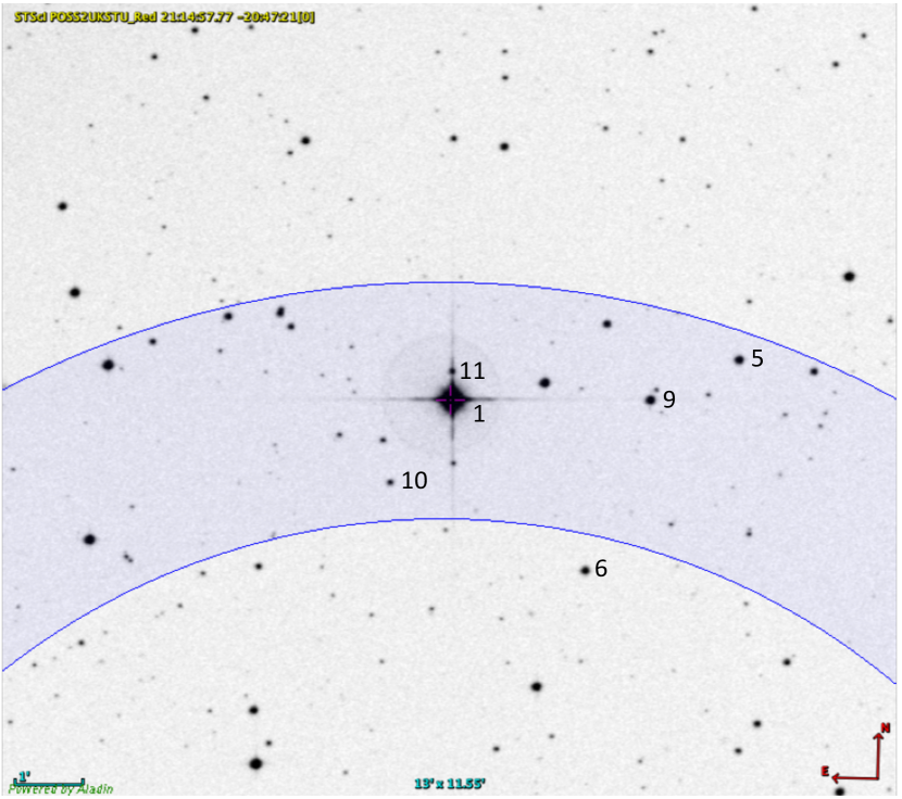
Figure 1: Positions within FGS 1r (blue-shaded region) of HD 202206 (1) and the astrometric reference stars (5 - 11) identified in Table 3. Note that due to HST roll restrictions, not all reference stars can be observed at each epoch. For example, ref-6 lies outside the FGS 1r  FOV at this epoch.

The astrometric reference frame for HD 202206 consists of five stars (Table 3). The HD 202206 field (Figure 1) exhibits the distribution of astrometric reference stars (ref-5 through ref-11) used in this study. The HD 202206 field was observed at a very limited range of spacecraft roll values (Table 2). Figure 2 shows the distribution in FGS 1r coordinates of the thirty-one sets (epochs) of HD 202206 and reference star measurements. HD 202206 (labeled ‘$\times$’) had to be placed in many different locations within the FGS 1r   total field of view (FOV) to maximize the number of astrometric reference stars in the FGS field of view and to insure guide star availability for the other two FGS units.  However, because the average radial distance of HD 202206 from FGS FOV center was $<r>=32"$, the astrometric impact of this displacement is indistinguishable from measurement noise. At each epoch we measured each reference stars 1 – 4 times, and HD 202206 3–5 times.

2.1.1 Modeling Priors

The success of single-field parallax astrometry depends on prior knowledge of the reference stars, and sometimes, of the science target. Catalog proper motions with associated errors, lateral color corrections, and estimates for reference star parallax are entered into the modeling as quasi-Bayesian priors, data with which to inform the final solved-for parameters. These values are not entered as hardwired quantities known to infinite precision. We include them as observations with associated errors. The model adjusts the corresponding parameter values within limits defined by the data input errors to minimize $\chi^{2}$, yielding the most accurate parallax and proper motion for the prime target, HD 202206, and the best opportunity to measure any reflex motion due to the companions detected by RV.

1. Reference Star Absolute Parallaxes- Because we measure the parallax of HD 202206 with respect to reference stars which have their own parallaxes, we must either apply a statistically-derived correction from relative to absolute parallax (van Altena et al., 1995, Yale Parallax Catalog, YPC95), or estimate the absolute parallaxes of the reference frame stars. We, again, choose the second option as we have since we first used it in Harrison et al. (1999). The colors, spectral type, and luminosity class of a star can be used to estimate the absolute magnitude, $M_{V}$, and $V$-band absorption, $A_{V}$. We estimate the absolute parallax for each reference star through this expression,

   $$\pi_{\rm abs}=10^{-(V-M_{V}+5-A_{V})/5}$$ (1)

   Our band passes for reference star photometry include: $BVRI$ photometry of the reference stars from the NMSU 1 m telescope located at Apache Point Observatory and JHK (from 2MASS). Table 4 lists the visible and infrared photometry for the HD 202206 reference stars.

   To establish spectral type and luminosity class, the reference frame stars were observed on 2009 December 9 using the RCSPEC on the Blanco 4 m telescope at CTIO. We used the KPGL1 grating to give a dispersion of 0.95 Å/pix. Classifications used a combination of template matching and line ratios. We determine the spectral types for the higher S/N stars to within $\pm$1 subclass. Classifications for the lower S/N stars have $\pm$2 subclass uncertainty. Table 5 lists the spectral types and luminosity classes for our reference stars. Note that we had no prior IR photometry or spectral information for reference star, ref-11 (just above and quite close to HD 202206 in Figure 1), hence no input prior parallax for the modeling.

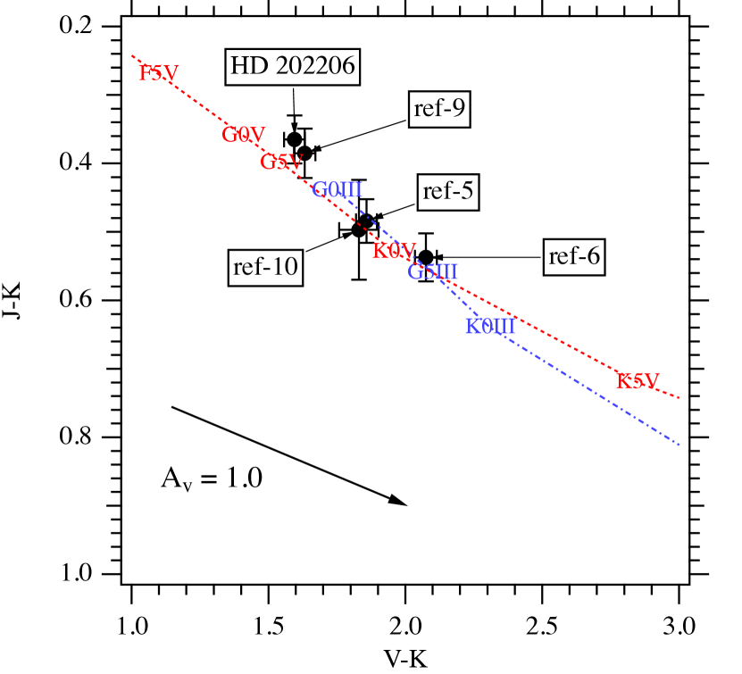
Figure 3: $(J-K)$ vs. $(V-K)$ color-color diagram for HD 202206 and astrometric reference stars identified in Table 4. The lines are the assumed (Cox, 2000) locus of dwarf (luminosity class V, dashed) and giant (luminosity class III, dot-dashed) stars of various spectral types. The reddening vector indicates $A_{V}=1.0$ for the plotted color systems. Along this line of sight maximum extinction is $A_{V}$$\sim$ 0.15 (Schlegel et al., 1998). There exists no 2MASS photometry for ref-11.

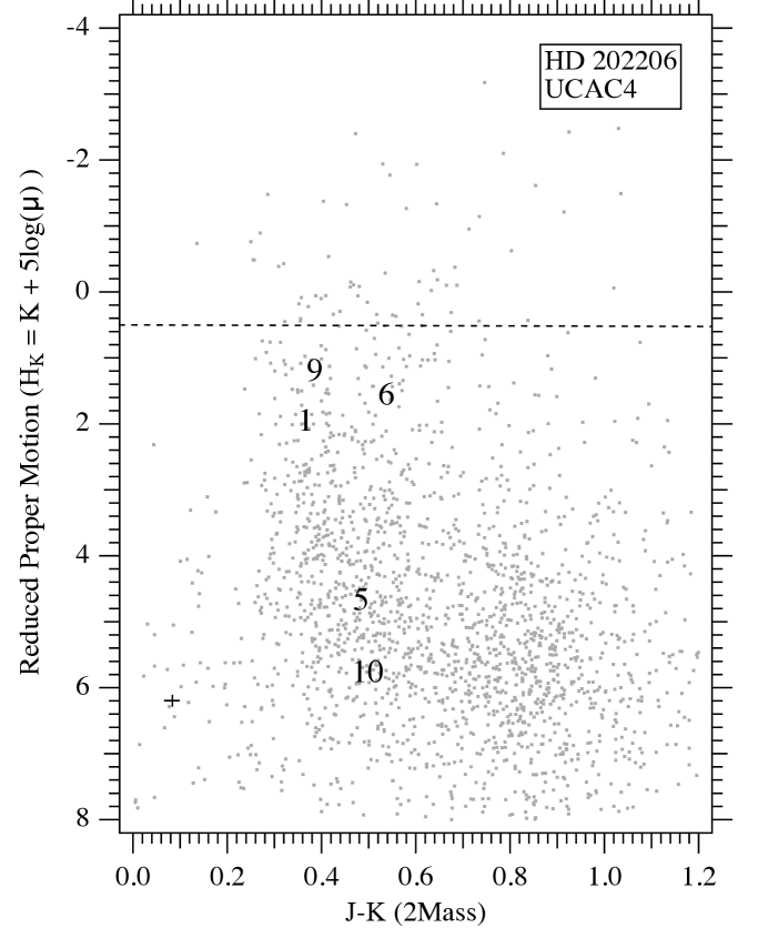
Figure 4: Reduced proper motion diagram for 2200 stars in a 1° field centered on HD 202206. Star identifications are in Table 4 and proper motions are from Tables 7 and 8. For a given spectral type, giants and sub-giants have more negative $H_{K}$ values and are redder than dwarfs in $(J-K)$. $H_{K}$ values are derived from proper motions in Table 7. The small cross at the lower left represents a typical $(J-K)$ error of 0.04 mag and $H_{K}$ error of 0.17 mag. Ref-11, omitted from the plot, lacks 2MASS photometry.  The horizontal line indicates a separation between dwarfs and sub-giant/giant stars.

   Figure 3 contains a $(J-K)$ vs. $(V-K)$ color-color diagram for HD 202206 and the reference stars. Schlegel et al. (1998) find an upper limit $A_{V}$$\sim$0.15 towards HD 202206, consistent with the small absorptions we infer comparing spectra and photometry (Table 5). The reference star derived absolute magnitudes critically depend on the assumed stellar luminosity, a parameter impossible to obtain for all but the latest type stars using only Figure 3. To check the luminosity classes obtained from classification spectra we obtain proper motions from the UCAC4 (Zacharias et al., 2013) for a one-degree-square field centered on HD 202206, and then produce a reduced proper motion diagram (Stromberg, 1939; Yong & Lambert, 2003; Gould & Morgan, 2003) to discriminate between giants and dwarfs. Figure 4 contains the reduced proper motion diagram for the HD 202206 field, including HD 202206 and our reference stars. We derive absolute parallaxes by comparing our estimated spectral types and luminosity class to $M_{V}$ values from Cox (2000).

   We adopted 1.0 mag input errors for distance moduli, $(m-M)_{0}$, for all reference stars. Contributions to the error are uncertainties in $A_{V}$ and errors in $M_{V}$ due to uncertainties in color to spectral type mapping. We list all reference star absolute parallax estimates in Table 5. Individually, no reference star absolute parallax is better determined than ${\sigma_{\pi}\over\pi}$ = 23%. The average input absolute parallax for the reference frame is $\langle\pi_{abs}\rangle=1.7$ mas. We compare this to the correction to absolute parallax discussed and presented in YPC95 (section 3.2, figure 2). Entering YPC95, figure 2, with the Galactic latitude of HD 202206 , $b=-40\arcdeg$, and average magnitude for the reference frame, $\langle V_{\rm ref}\rangle=14.94$, we obtain a correction to absolute of 1.5 mas, consistent with our derived correction.

2. Proper Motions- We use proper motion priors from the UCAC4 Catalog (Zacharias et al., 2013). These quantities typically have errors on order 4 mas yr^-1.

3. Lateral Color Corrections-  To effectively periscope the entire FGS FOV, the FGS design includes refractive optics. Hence, a blue star and a red star at exactly the same position on the sky would be measured to have different positions. A series of observations of pairs of red and blue stars with small angular separation at various spacecraft roll positions yields the required corrections. The discussion in section 3.4 of Benedict et al. (1999) describes how we derive this correction for FGS 3. A similar analysis resulted in FGS 1r lateral color corrections $lc_{x}=-0.83\pm 0.11$ mas and $lc_{y}=-0.8\pm 0.08$ mas, quantities introduced as observations with error in the model shown below. These corrections have very little impact on the final results, given the small spread in $B-V$ color (Table 4) between HD 202206 and the reference stars.

2.2 The Astrometric Model

While the HD 202206 usable reference frame contains five stars, due to guide star availability we average four observed reference stars stars per epoch. From positional measurements we determine the scale, rotation, and offset “plate constants” relative to an arbitrarily adopted constraint epoch for each observation set. We employ GaussFit (Jefferys et al. 1988) to minimize $\chi^{2}$. The solved equations of condition for the HD 202206 field are:

$$x^{\prime}=x+lc_{x}(\it B-V)$$ (2)

$$y^{\prime}=y+lc_{y}(\it B-V)$$ (3)

$$\xi=\overline{A}x^{\prime}+\overline{B}y^{\prime}+\overline{C}-\mu_{\alpha}\Delta t-P_{\alpha}\pi-(ORBIT_{B,x}+ORBIT_{c,x})$$ (4)

$$\eta=-\overline{B}x^{\prime}+\overline{A}y^{\prime}+\overline{F}-\mu_{\delta}\Delta t-P_{\delta}\pi-(ORBIT_{B,y}+ORBIT_{c,y})$$ (5)

Identifying terms, $\it x$ and $\it y$ are the measured coordinates from HST; $(B-V)$ is the Johnson $(B-V)$ color of each star; and $\it lc_{x}$ and $\it lc_{y}$ are the lateral color corrections, which have little impact due to the small range of color for HD 202206 and reference stars (Table 4).  $\overline{A}$, and $\overline{B}$ are scale and rotation plate constants, $\overline{C}$ and $\overline{F}$ are offsets; $\mu_{\alpha}$ and $\mu_{\delta}$ are proper motions; $\Delta t$ is the time difference from the constraint epoch; $P_{\alpha}$ and $P_{\delta}$ are parallax factors; and $\it\pi$ is the parallax. Note that we apply no cross-filter corrections (c.f. Benedict et al. 2007) because HD 202206 is faint enough that the FGS 1r F5ND neutral density filter is unnecessary.

We obtain the parallax factors from a JPL Earth orbit predictor (Standish 1990), version DE405. We obtain an orientation to the sky for the FGS 1r constraint plate (set 11 in Table 2) from ground-based astrometry (the UCAC4 Catalog) with uncertainties of $0\fdg 06$.

$ORBIT_{x}$ and $ORBIT_{y}$ are functions of the classic parameters $\alpha$, the perturbation semi major axis, $i$, inclination, $e$, eccentricity, $\omega$, argument of periastron, $\Omega$, longitude of ascending node, $P$, orbital period, and $T_{0}$, time of periastron passage (Heintz, 1978; Martioli et al., 2010). We model a sequence of measures of the host star motion (including parallax, proper motion and perturbations) relative to the reference frame seen in Figure 1.

The elliptical rectangular coordinates $x$,$y$, of the unit orbit are

$$x = (\cos{E}-e)$$ (6)

$$y = \sqrt{1-e^{2}}\sin{E}$$ (7)

with eccentricity, $e$, and $E$, the eccentric anomaly. $E$ depends on time, $t$, through Kepler’s equation,

$$\frac{2\pi}{P}(t-T_{0})=E-e\sin{E}$$ (8)

with epoch of periastron passage, $T_{0}$, and the orbital period, $P$. The eccentric anomaly, $E$ relates to the true anomaly, $f$, through

$$\tan{\frac{f}{2}}=\sqrt{\frac{1+e}{1-e}}\tan{\frac{E}{2}}$$ (9)

The projection of this true orbit onto a plane tangent to the sky yields the coordinates $ORBIT_{x}$, $ORBIT_{y}$

$$ORBIT_{x} = Bx+Gy$$ (10)

$$ORBIT_{y} = Ax+Fy$$ (11)

with Thiele-Innes constants;  $B_{TI},A_{TI},G_{TI},F_{TI}$

$$B_{TI} = \alpha(\cos{\omega}\sin{\Omega}+\sin{\omega}\cos{\Omega}\cos{i})$$ (12)

$$A_{TI} = \alpha(\cos{\omega}\cos{\Omega}-\sin{\omega}\sin{\Omega}\cos{i})$$ (13)

$$G_{TI} = \alpha(-\sin{\omega}\sin{\Omega}+\cos{\omega}\cos{\Omega}\cos{i})$$ (14)

$$F_{TI} = \alpha(-\sin{\omega}\cos{\Omega}-\cos{\omega}\sin{\Omega}\cos{i})$$ (15)

$ORBIT_{x}$ and $ORBIT_{y}$ denote the coordinates of the parent star around the barycenter. For HD 202206 the FGS detects and characterizes a superposition of the perturbation sizes, $\alpha_{B}$ and $\alpha_{c}$ due to components B and c, through $(ORBIT_{B,x}+ORBIT_{c,x})$ and $(ORBIT_{B,y}+ORBIT_{c,y})$.

2.3 The RV Model

Udry et al. (2002); Correia et al. (2005); Couetdic et al. (2010) measured the radial component of the stellar orbital motion around the barycenter of the system with Doppler spectroscopy. This changing velocity, $v$, is the projection of a Keplerian orbital velocity to the observer’s line of sight plus a constant velocity $\gamma$. Therefore, for components B and c

$$v_{B}=\gamma+K_{B}[\cos{(f_{B}+\omega_{B})}+e_{B}\cos{\omega_{B}}]$$ (16)

$$v_{c}=\gamma+K_{c}[\cos{(f_{B}+\omega_{c})}+e_{c}\cos{\omega_{c}}]$$ (17)

$$v_{tot}=v_{B}+v_{c}$$ (18)

where $K$ is the velocity semi-amplitude. The total RV signal (Couetdic et al., 2010) we model ($v_{tot}$) includes contributions from both components B and c.

2.4 Determining Perturbation Orbits for HD 202206 B and c

To derive companion perturbation orbital elements we simultaneously model RV values from Couetdic et al. (2010) and HST astrometry (Table 2). Because our GaussFit modeling results critically depend on the input data errors, we first modeled only the RV (Equation 18) to assess the validity of the original (Couetdic et al., 2010) input RV errors. Solving for the orbital parameters of components B and c, to achieve a $\chi^{2}/$DOF of unity, where DOF represents the degrees of freedom in the solution, required increasing the original errors by a factor of 1.4.

Tables 7 and 8 list results of this modeling; the proper motions (relative), absolute parallaxes, and absolute magnitudes and their errors (1-$\sigma$) for the five reference stars and HD 202206. Table 9 contains final orbit parameter values and errors for a model including both RV and astrometry; the period ($P$), the epoch of passage through periastron in years ($T$), the eccentricity ($e$), and the angle in the plane of the true orbit between the line of nodes and the major axis ($\omega$), are the same for an orbit determined from RV or from astrometry. The remaining orbital elements ($i,\Omega,\alpha$) come only from astrometry. Our model allows the astrometry and the RV to describe two companions, HD 202206 B and c. Astrometry and RV are forced to describe the same system through this constraint (Pourbaix & Jorissen, 2000), shown for component B, though in the model applied to both the B and c components,

$${{\alpha_{B}~{}sin\,i_{B}\over\pi_{abs}}={P_{B}K_{B}(1-e_{B}^{2})^{1/2}\over 2\pi\times 4.7405}}$$ (19)

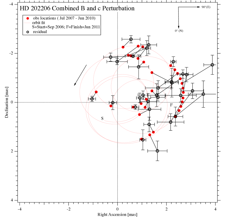
Figure 7: Residuals to the combined B,c perturbation described by the Table 9 final orbital elements. Normal points (o) for each Table 2 epoch (unique set number) attach to their calculated locations ($\bullet$) on the combined orbit (- -), representing 4.8 years from September 2006 to July 2011. Actual observations spanned July 2007 to June 2010. Residual RMS is 0.35 mas in RA, 0.32 mas in DEC. Errors are the standard deviation of the mean for each normal point, typically comprised of 5 separate observations per set.

where quantities derived only from astrometry (parallax, $\pi_{abs}$, host star perturbation orbit size, $\alpha$, and inclination, $i$) are on the left, and quantities derivable from both (the period, $P$ and eccentricity, $e$), or radial velocities only (the RV amplitude of the primary, $K$, induced by a companion), are on the right. Given the sparse orbit coverage of the HD 202206 B and especially the c perturbation afforded by the astrometry (Figures 7 and 8), the RV data were essential in determining the component orbits. For most of the orbital parameters in Table 9 a combination of astrometry and previously existing RV has reduced the Correia et al. (2005); Couetdic et al. (2010) formal errors.

2.5 Assessing Modeling Residuals

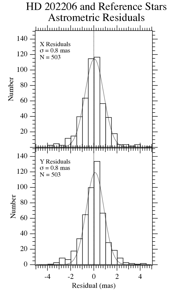
Figure 5: Histograms of x and y residuals obtained from modeling the FGS observations of HD 202206 and the FGS reference frame with Equations 2 – 5. Distributions are fit with gaussians with standard deviations, $\sigma$, indicated in each panel.

From histograms of the FGS astrometric residuals (Figure 5) we conclude that we have a well-behaved solution exhibiting residuals with Gaussian distributions with dispersions $\sigma\sim 0.8$ mas.  The slight skew in the Y residuals can be seen in either X or Y residuals, either positive or negative in many previous modelings, e.g. Benedict et al. (2009, 2010, 2011); McArthur et al. (2011); Benedict et al. (2016) with no discernable impact on results. The reference frame ’catalog’ from FGS 1r in $\xi$ and $\eta$ standard coordinates (Table 6) was determined with average uncertainties, $\langle\sigma_{\xi}\rangle=0.26$ and $\langle\sigma_{\eta}\rangle=0.22$ mas. Because we have rotated our constraint plate to an RA, DEC coordinate system, $\xi$ and $\eta$ are RA and DEC.

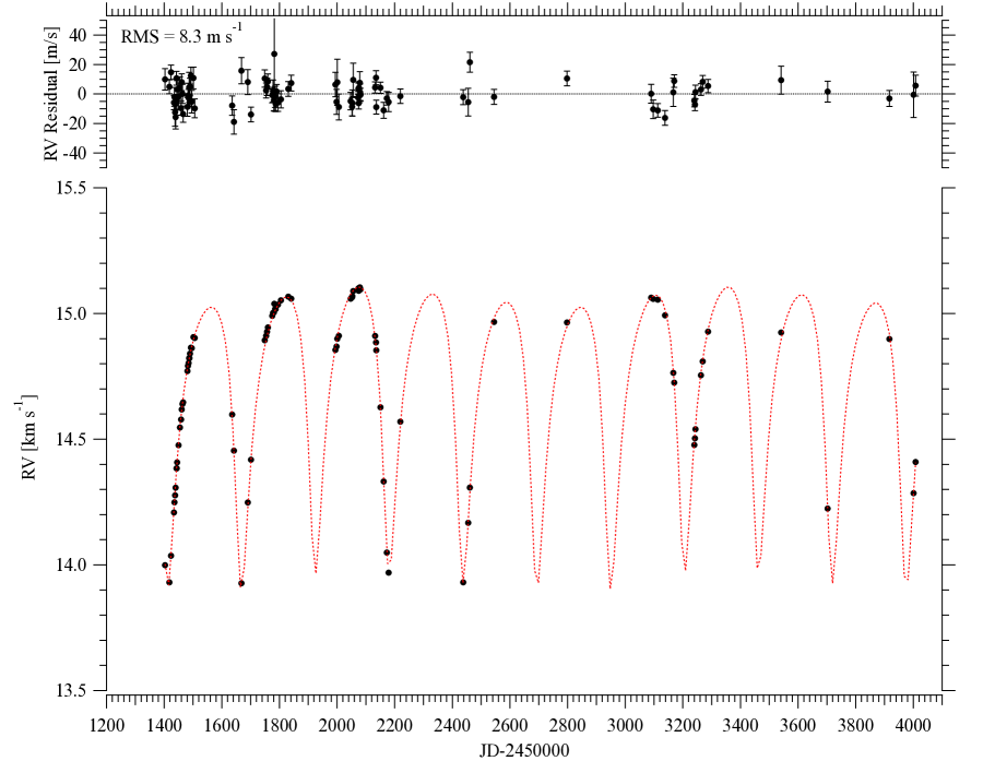
Figure 6: RV values from Couetdic et al. (2010) and the final RV two component orbit (Table 9) obtained from modeling the RV and the FGS observations of HD 202206 and the FGS reference frame with Equations 2 – 5. The original RV errors (Couetdic et al., 2010) have been increased by a factor of 1.4 to achieve a unity $\chi^{2}$. Residuals are plotted in the top panel tagged with the adopted RV errors. We note the RMS residual value in the plot.

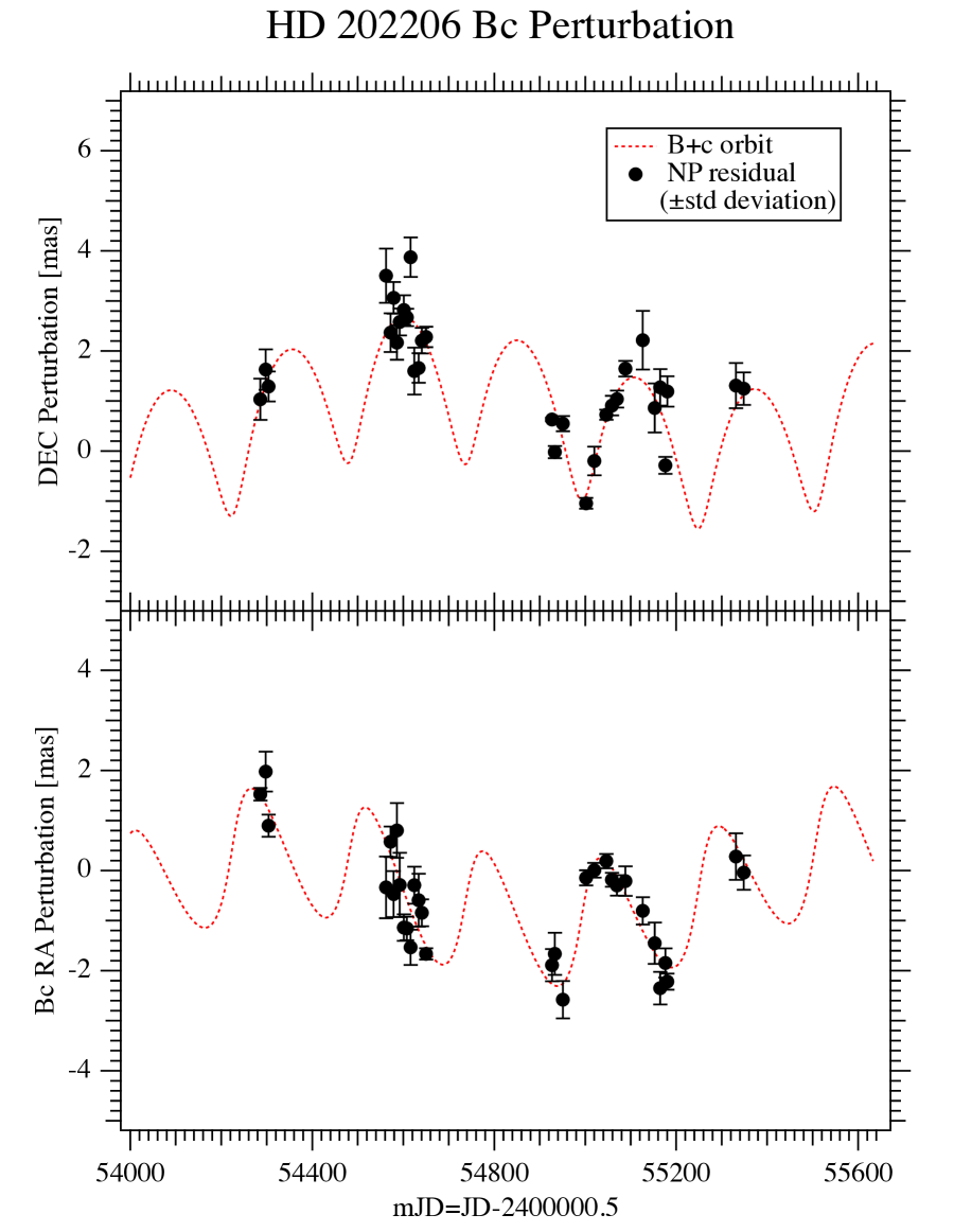
Figure 8: Time variation of the RA and DEC components of the perturbation (- -) described by the Table 9 final orbital elements over-plotted with normal points ($\bullet$) for each Table 2 epoch (unique set number). Errors are the same as for Figure 7.

At this stage we can assess the quality of the HD 202206 B and HD 202206 c astrometric perturbations by plotting the RV and astrometric residuals from our modeling of the component B,c orbit. We show the RV orbit with adopted errors and final residuals to the simultaneous modeling in Figure 6. Figure 7 shows the RA and DEC components at each observational epoch (the 31 data sets listed in Table 2) plotted on the final component B,c orbit. We plot averages of FGS residuals at each epoch plotted as small symbols, connected to their calculated position on the orbit. These normal point residuals have an average absolute value residual, $\langle|residual|\rangle=0.34$ mas. Figure 8 shows our average (typically five positions) measures for each Table 2 data set with associated standard deviation of the mean plotted on the RA and DEC components of the combined B,c orbit described by the model-derived orbital elements in Table 9.

3 Masses and Mutual Inclination

For the parameters critical in determining the masses of the companions to HD 202206 we find a parallax, $\pi_{abs}=21.96\pm 0.12$ mas and a proper motion in RA of $-41.54\pm 0.11$ mas y^-1 and in DEC of $-117.87\pm 0.11$ mas y^-1. Table 8 compares values for the parallax and proper motion of HD 202206 from HST, Gaia (Brown, Anthony G.A. & Collaboration, 2016), and the Hipparcos re-reduction (van Leeuwen, 2007). While the parallax values agree within their respective errors, we note a small disagreement in the proper motion vector ($\vec{\mu}$) absolute magnitude and direction. This could be explained by our non-global proper motion measured against a small sample of reference stars. Our measurement precision and extended study duration have significantly improved the precision of the parallax of HD 202206.

For the perturbation due to component B we find $\alpha_{B}=1.4\pm 0.1$ mas, and an inclination, $i_{B}$= 10$\fdg$9 $\pm$ 0$\fdg$8. We find $\alpha_{c}=0.76\pm 0.11$ mas, and an inclination, $i_{c}$= 7$\fdg$7 $\pm$ 1$\fdg$1. We list all modeled orbital elements in Table 9 with 1-$\sigma$ errors. The mutual inclination, $\Phi$, of the B and c orbits can be determined through (Kopal, 1959; Muterspaugh et al., 2006)

$$cos\,\Phi=cos\,i_{B}cos\,i_{c}+sin\,i_{B}sin\,i_{c}cos(\Omega_{B}-\Omega_{c})$$ (20)

where $i_{B}$ and $i_{c}$ are the orbital inclinations and $\Omega_{B}$ and $\Omega_{c}$ are the longitudes of their ascending nodes. Our modeling yields a suggestion of coplanarity with $\Phi=6\pm 2\arcdeg$.

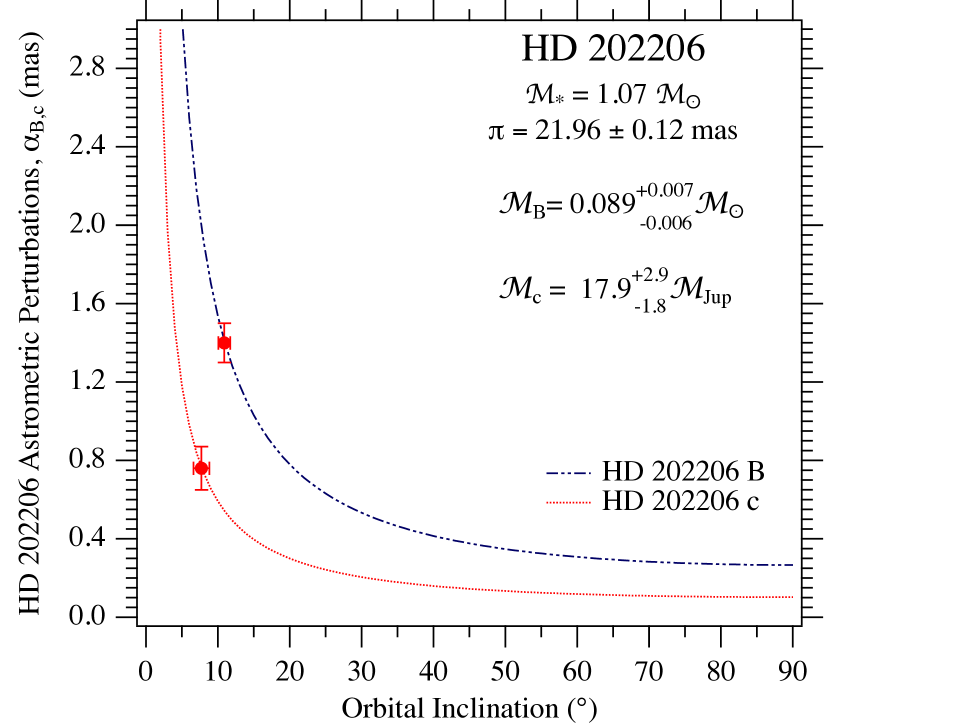
Figure 9: These curves relate perturbation size and inclination for HD 202206 B and c through the Pourbaix & Jorrisen (2000) relation (Equation 19). For each component we use the curve as a ‘prior’ in a quasi-bayesian sense. Our final values for the semimajor axes of the astrometric perturbations, $\alpha_{B}$, $\alpha_{c}$ and inclinations, $i_{B}$, $i_{c}$ are plotted with their formal errors.

Figure 9 illustrates the Pourbaix and Jorrisen relation (Equation 19) between parameters obtained from astrometry and RV and our final estimates for each component $\alpha$ and $i$. In essence, our simultaneous solution uses the Figure 9 component B and c curves as quasi-Bayesian priors, sliding along them until the astrometric residuals and orbit parameter errors are minimized.

The planetary mass depends on the mass of the primary star, for which we have adopted $\cal{M}$_∗=1.07 $\cal{M}_{\odot}~{}$(Han et al., 2014). We find $\cal{M}$${}_{B}=93.6^{+7.7}_{-6.6}$$\cal{M}_{\rm Jup}$ = $0.089^{+0.007}_{-0.006}$ $\cal{M}_{\odot}$. The central mass controlling the component c orbit is now the sum of the component A and B masses, $\cal{M}$${}_{A+B}=1.16$$\cal{M}_{\odot}$. Hence, for component c, $\cal{M}$${}_{c}=17.9^{+2.9}_{-1.8}$$\cal{M}_{\rm Jup}$. In Table 9 the final mass values for components B and c do not incorporate the present uncertainty in the stellar mass, $\cal{M}$_∗.

Table 8 shows the FGS proper motion to have a small disagreement with previously measured Hipparcos  and Gaia  values. Our modeling can include any priors, but we generally resist including priors for the prime scientific target. If we include HD 202206 proper motion priors (and estimated errors) from Hipparcos (van Leeuwen, 2007), Gaia (Brown, Anthony G.A. & Collaboration, 2016), the PPMXL (Roeser et al., 2010), UCAC4 (Zacharias et al., 2013), and SPM 4.0 (Girard et al., 2011) catalogs, we obtain a proper motion in agreement with the Gaia value. The resulting masses and mutual inclinations of components B and c agree within the Table 9 errors. However, the $\chi^{2}$ increases by 5.2%, while the degrees of freedom increase by 1.1%. Hence, we prefer the Table 9 results from a solution without HD 202206 proper motion priors.

4 Discussion

From the Benedict et al. (2016) Mass-Luminosity relations we can estimate absolute magnitudes for an M dwarf star with mass $\cal{M}$= 0.089 $\cal{M}_{\odot}$. Those relations yield $M_{V}=17.80$ and $M_{K}=9.79$. Our parallax, $\pi_{abs}=21.96$, and an interstellar absorption, $A_{V}=0$, provide a distance modulus, $(m-M)_{0}=3.30$, and for the host star HD 202206 $M_{V}=4.77$ and $M_{K}=3.19$. HD 202206 B at apastron has a separation $\rho_{B}=a_{B}(1+e_{B})=26.1$ mas with $\Delta V=13.0$ and $\Delta K=6.6$, a challenging upcoming (March-December 2019) test for any existing high-contrast imaging system.

Our characterization of the HD 202206 system comes close to providing a solution to the vexing problem of stability. With only $\cal{M}$ sin i values for components b and c Correia et al. (2005); Couetdic et al. (2010); Petrovich (2015) argued that a stable HD 202206 system should be in a 5:1 mean motion resonance (MMR) and coplanar. Our re-determination of the periods (listed in Table 9) yield $P_{c}/P_{B}=4.92\pm 0.04$, a value less than 3-$\sigma$ from MMR. Our mutual inclination, $\Phi=6\pm 2\arcdeg$, differs from coplanarity by 3-$\sigma$.

Our modeling platform, GaussFit, easily accommodates any priors as data with associated errors. Given that stability seems to require a 5:1 MMR, we constructed a model that includes a new piece of ‘data’, $Pdiff$, a new parameter, $Ppdiff$, and the associated equation of condition relating the two

$$Pdiff=(P_{B}*5.0)-P_{c}$$ (21)

$$value=Ppdiff-Pdiff$$ (22)

This addition to our model introduces the period ratio, $P_{c}/P_{B}=5$, as a prior constraint, where the observable derived from theory is $Pdiff=0\pm 20$ days, and $value$ is the quantity to be minimized (in $\chi^{2}$) by the modeling. The adopted error for $Pdiff$ represents a 1.7% difference in the expected 5:1 MMR. We present the orbital parameters and component masses resulting from that modeling in Table 10, which now includes the parameter, $Ppdiff=3\pm 5$ days, effectively zero, suggesting a 5:1 MMR. The component masses are a little higher, but agree within the errors with those (Table 9) resulting from a model with no prior knowledge of a possibly required resonance. The parallax and proper motions were unchanged from the Table 8 values. The assertion of a 5:1 MMR has forced a higher degree of coplanarity, i.e., the smaller $\Phi$ value shown in Table 10.

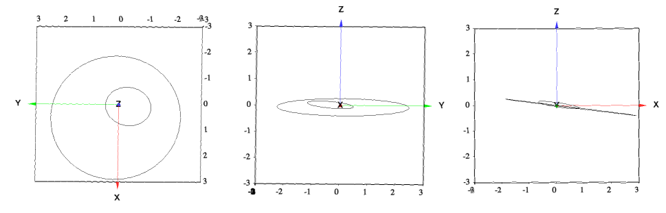
Figure 10: Component B (inner) and c (outer) orbits as observed (left to right panels) towards the -z (looking at the HD 202206 system with +y to the south and +x pointing west), towards -x (east in RA), and -y (north in DEC) axes. Axes units are AU.

Finally, we plot component B and c actual orbits (in AU, from the Table 9 parameters) in Figure 10 from three vantage points; as seen on the sky (along the z axis), and plots looking north towards -y and east in the direction of -x. These views demonstrate the degree of coplanarity (without prior knowledge of a coplanarity requirement) determined through our modeling.

5 Summary

For the HD 202206 system we find

1. A parallax, $\pi_{abs}=21.96\pm 0.12$ mas, agreeing with the Hipparcos and $Gaia$ values within the errors,

2. A relative, not absolute proper motion relative to our reference frame, $\vec{\mu}=124.98$ mas yr^-1 with a position angle, P.A. = $199\fdg 4$, differing by 1.5 mas yr^-1 and $1\fdg 3$ compared to $Gaia$,

3. An inclination for HD 202206 B , $i_{B}$= 10$\fdg$9 $\pm$ 0$\fdg$8 and, with the assumption of a HD 202206 A mass, $\cal{M}$_A = 1.07 $\cal{M}_{\odot}~{}$, a component B mass, $\cal{M}$${}_{B}=0.089^{+0.007}_{-0.006}$ $\cal{M}_{\odot}$. HD 202206 B is an  M8 dwarf star (Dupuy & Liu, 2017),

4. A component c inclination, $i_{c}=7\fdg 7\pm 1\fdg 1$, that with a central mass now $\cal{M}$${}_{A+B}=1.16$ $\cal{M}_{\odot}~{}$, yields a component c mass, $\cal{M}$${}_{c}=17.9^{+2.9}_{-1.8}$$\cal{M}_{\rm Jup}$. HD 202206 c is a brown dwarf,

5. A period ratio $P_{c}/P_{B}=4.92\pm 0.04$, near a 5:1 MMR, and a flat HD 202206 system architecture with a B-c mutual inclination of $\Phi=6\arcdeg\pm 2\arcdeg$, near coplanarity,

6. That including proper motion priors from multiple sources yields the same component B and component c masses as ignoring those priors,

7. That including a 5:1 MMR as a prior yields the same component B and component c masses as ignoring that prior, while nudging the HD 202206 system slightly closer to coplanarity, with $\Phi=4\arcdeg\pm 2\arcdeg$.

Thus the question posed in the title of the Correia et al. (2005) paper, “A pair of planets around HD 202206 or a circumbinary planet?”, is answered with a single word; neither. The HD 202206 system consists of a low-inclination, nearly face-on G8V + M6V binary orbited by a brown dwarf.

A combination of additional RV measurements and Gaia astrometry should further illuminate our understanding of the dynamics of this interesting system, particularly by reducing the errors on periods and coplanarity. We repeat an old question: is the HD 202206 system stable, or just close to stable?

Table 1: HD 202206 Stellar Parameters

Parameter	Value	Source
SpT	G6V	1
Teff	5766 K	6
log g	4.5 $\pm$ 0.1	4
$[Fe/H]$	0.3 $\pm$ 0.1	6
age	2.9 $\pm$ 1.0 Gy	5
mass	1.07 $\pm$ 0.08 $\cal{M}_{\sun}$	4
distance	45.5 $\pm$ 0.3 pc	2
AV	0.0	1
Radius	1.04 $\pm$ 0.01$R_{\sun}$	5
v sin i	2.3 $\pm$ 0.5 km s-1	4
m-M	3.30$\pm$ 0.01	2
$V$	8.07 $\pm$ 0.01	1
$K$	6.49 $\pm$ 0.02	3
$V-K$	1.58 $\pm$ 0.03	1,3

¹SIMBAD,⁴Exoplanets Website (Han et al., 2014), ²this paper,
³2MASS, ⁵Bonfanti et al. (2016), ⁶Hinkel et al. (2016).

Table 2: HD 202206 Field Astrometry

Set	Star	HSTID	V	V3 roll	X	Y	$\sigma_{X}$	$\sigma_{Y}$	tobs	Pα	Pδ
1	1	F9YM0102M	8.2	280.612	-5.3808719	2.5181351	0.0024	0.0030	54285.60839	0.579256385	0.098856994
1	5	F9YM0103M	14.41	280.612	232.7332958	-81.5462095	0.0035	0.0030	54285.60979	0.578137858	0.098769874
1	9	F9YM0105M	13.96	280.612	163.6020442	-32.1472399	0.0035	0.0038	54285.61266	0.578449648	0.098684625
1	5	F9YM0106M	14.42	280.612	232.7333590	-81.5463100	0.0035	0.0045	54285.61403	0.578059536	0.098753214
1	11	F9YM0108M	15.8	280.612	-11.4354866	-23.3057775	0.0037	0.0040	54285.61709	0.579074299	0.098937542
1	5	F9YM0109M	14.44	280.612	232.7329783	-81.5462846	0.0036	0.0053	54285.61858	0.577974028	0.098734923
1	1	F9YM010AM	8.2	280.612	-5.3805110	2.5179985	0.0028	0.0059	54285.61983	0.579044335	0.098811176
1	5	F9YM010BM	14.42	280.612	232.7339517	-81.5449234	0.0033	0.0038	54285.62132	0.577923291	0.098723367
1	5	F9YM010CM	14.43	280.612	232.7326276	-81.5462801	0.0037	0.0041	54285.62263	0.577899611	0.098717663
1	9	F9YM010DM	13.97	280.612	163.6020574	-32.1466724	0.0033	0.0034	54285.62382	0.578243003	0.098638334
1	11	F9YM010EM	15.79	280.612	-11.4345429	-23.3038134	0.0036	0.0038	54285.62524	0.578926197	0.098902322
1	1	F9YM010FM	8.2	280.612	-5.3807179	2.5170693	0.0024	0.0035	54285.62623	0.578930526	0.098782607
1	5	F9YM010GM	14.42	280.612	232.7327101	-81.5468546	0.0036	0.0031	54285.62767	0.577812914	0.098694251
2	1	F9YM0301M	8.2	253.022	1.8980570	-45.9885308	0.0015	0.0015	54297.38964	0.400934043	0.038705436
2	5	F9YM0302M	14.42	253.022	251.8340113	-10.0603051	0.0026	0.0017	54297.39127	0.399679689	0.038708685
…	…	…	…	…	…	…	…	…	…	…	…

Table 3: Astrometric Reference Stars

ID	RA    (J2000.0)	DEC	V
5	318.666441	-20.778502	14.30
6	318.705720	-20.830115	14.54
9	318.689335	-20.788494	13.95
10	318.756629	-20.809268	15.98
11	318.740855	-20.782022	15.92

Table 4: Visible and Near-IR Photometry

ID	$V$	$B-V$	$K$	$(J-H)$	$(J-K)$	$(V-K)$
1	8.08$\pm$0.03	0.72$\pm$0.03	6.485$\pm$0.023	0.283$\pm$0.031	0.365$\pm$0.035	1.60$\pm$0.04
5	14.30 0.03	0.73 0.10	12.442 0.023	0.423 0.034	0.484 0.032	1.86 0.04
6	14.00 0.03	0.74 0.05	12.465 0.026	0.456 0.033	0.537 0.035	2.08 0.04
9	13.95 0.03	0.70 0.05	12.318 0.025	0.330 0.034	0.385 0.036	1.63 0.04
10	15.98 0.03	0.65 0.09	14.150 0.066	0.255 0.064	0.497 0.073	1.83 0.07
11	15.92 0.10	0.87 0.09

Table 5: Astrometric Reference Star Initial Spectrophotometric Parallaxes

ID	Sp. T.	V	MV	m-M	AV	$\pi_{abs}$(mas)
5	K1.5V	14.30	6.3	8.0	0.00	2.5$\pm$0.6
6	K0V	14.54	5.9	8.6	0.00	1.9 0.4
9	G5V	13.95	5.1	8.9	0.06	1.6 0.4
10	G5V	15.98	5.1	10.9	0.00	0.7 0.2

Table 6: HD 202206 and Reference Star Relative Positions

Star	V	$\xi$	$\eta$
1	8.08	0.19070$\pm$0.00013	20.77968$\pm$0.00014
5	14.3	-249.19116 0.00011	60.23407 0.00007
6	14.54	-117.09436 0.00046	-125.45195 0.00032
9	13.95	-172.23627 0.00018	24.24109 0.00015
10	15.98	54.06826 0.00052	-50.63166 0.00047
11	15.92	1.50403 0.00018	47.38927 0.00017

Table 7: Reference Star Final Proper Motions, Parallaxes, and Absolute Magnitudes

ID	V	$\mu_{\alpha}$	$\mu_{\delta}$	$\pi_{abs}$	MV
5	14.3	-6.66$\pm$0.10	-22.63$\pm$0.11	2.35$\pm$0.13	6.15$\pm$0.05
6	14.54	3.00 0.45	-9.43 0.50	1.93 0.10	5.96 0.05
9	13.95	-11.29 0.16	-14.28 0.17	1.74 0.13	5.09 0.07
10	15.98	-13.69 0.40	-8.05 0.42	0.67 0.04	5.10 0.05
11	15.92	3.95 0.17	-0.72 0.19	1.08 0.06	6.08 0.05

Table 8: Reference Frame Statistics, HD 202206 Parallax, and Proper Motion

Parameter	Value
Study duration	2.91 y
number of observation sets	31
reference star $\langle V\rangle$	14.94
reference star $\langle(B-V)\rangle$	0.79
HST Absolute $\pi$	21.96 $\pm$ 0.12 mas
Relative $\mu_{\alpha}$	-41.54 $\pm$ 0.11 mas yr-1
Relative $\mu_{\delta}$	-117.87 $\pm$ 0.11 mas yr-1
$\vec{\mu}=124.98$ mas yr-1
P.A. = $199\fdg 4$
Gaia DR1 Absolute $\pi$	21.94 $\pm$ 0.26 mas
Absolute $\mu_{\alpha}$	-39.22 $\pm$ 0.07 mas yr-1
Absolute $\mu_{\delta}$	-120.29 $\pm$ 0.04 mas yr-1
$\vec{\mu}=126.53$ mas yr-1
P.A. = $198\fdg 1$
HIP07 Absolute $\pi$	22.06 $\pm$ 0.82 mas
Absolute $\mu_{\alpha}$	-38.40 $\pm$ 0.94 mas yr-1
Absolute $\mu_{\delta}$	-119.81 $\pm$ 0.37 mas yr-1
$\vec{\mu}=125.81$ mas yr-1
P.A. = $197\fdg 8$

Table 9: Orbital Elements for the HD 202206 B and c Perturbations

Parameter	Units	B	err	c	err
P	days	256.33	0.02	1260	11
P	years	0.70180	0.00005	3.45	0.03
$T_{0}$	JD-2400000	52176.14	0.12	53103	452
e	-	0.432	0.001	0.22	0.03
K	km s-1	0.567	0.001	0.041	0.001
i	$\arcdeg$	10.9	0.8	7.7	1.1
$\omega$	$\arcdeg$	161.9	0.2	280	4
$\Omega$	$\arcdeg$	121	4	91	11
$\alpha$	mas	1.40	0.10	0.76	0.11
Derived Parameters
$\alpha$	AU	0.064	0.005	0.035	0.005
a	AU	0.83		2.41
a	mas	18.2		52.9
$\cal{M}$ sin i	$\cal{M}_{\rm Jup}$	17.7		2.3
$\cal{M}$	$\cal{M}_{\rm Jup}$	93.6	${}^{+7.7}_{-6.6}$	17.9	${}^{+2.9}_{-1.8}$
$\cal{M}$	$\cal{M}_{\odot}~{}$	0.089		0.017
Stability Parameters
$P_{c}/P_{B}$	-	4.92	0.04
$\Phi$	$\arcdeg$	6	2

Table 10: Orbital Elements with 5:1 MMR Prior

Parameter	Units	B	err	c	err
P	days	256.31	0.02	1278	6
P	years	0.70174	0.00004	3.50	0.02
$T_{0}$	JD-2400000	52176.10	0.11	53109	223
e	-	0.432	0.001	0.20	0.03
K	km s-1	0.567	0.001	0.041	0.001
i	$\arcdeg$	10.8	0.8	7.7	1.1
$\omega$	$\arcdeg$	161.9	0.2	280	4
$\Omega$	$\arcdeg$	121	4	100	9
$\alpha$	mas	1.40	0.10	0.76	0.11
Derived Parameters
$\alpha$	AU	0.064	0.005	0.035	0.005
a	AU	0.83		2.43
a	mas	18.2		53.4
$\cal{M}$ sin i	$\cal{M}_{\rm Jup}$	17.7		2.3
$\cal{M}$	$\cal{M}_{\rm Jup}$	93.9	${}^{+7.6}_{-6.5}$	18.0	${}^{+2.9}_{-2.0}$
$\cal{M}$	$\cal{M}_{\odot}~{}$	0.090		0.017
Stability Parameters
Period ratio, $P_{c}/P_{B}$	-	4.99	0.02
$Ppdiff$	days	3	5
$\Phi$	$\arcdeg$	4	2

Figure 2: Positions of HD 202206 (HD) and astrometric reference stars (5 –11) in FGS 1r  FOV coordinates. Due to guide star availability it was not possible to keep HD 202206 in the  FOV center at each epoch,  but the distance from the FOV center always remained $\leq 100$ seconds of arc, with an average distance, $<r>=32"$.

References

- Benedict (2007) Benedict G., 2007. The Architecture of Exoplanetary Systems. HST Proposal #11210
- Benedict et al. (2016) Benedict G.F., Henry T.J., Franz O.G., et al., 2016. AJ, 152, 141
- Benedict et al. (1999) Benedict G.F., McArthur B., Chappell D.W., et al., 1999. AJ, 118, 1086
- Benedict et al. (2010) Benedict G.F., McArthur B.E., Bean J.L., et al., 2010. AJ, 139, 1844
- Benedict et al. (2007) Benedict G.F., McArthur B.E., Feast M.W., et al., 2007. AJ, 133, 1810
- Benedict et al. (2011) Benedict G.F., McArthur B.E., Feast M.W., et al., 2011. AJ, 142, 187
- Benedict et al. (2009) Benedict G.F., McArthur B.E., Napiwotzki R., et al., 2009. AJ, 138, 1969
- Benedict et al. (2017) Benedict G.F., McArthur B.E., Nelan E.P., et al., 2017. PASP, 129, 012001
- Bonfanti et al. (2016) Bonfanti A., Ortolani S., & Nascimbeni V., 2016. A&A, 585, A5
-
Brown, Anthony G.A. & Collaboration (2016)
Brown, Anthony G.A. & Collaboration, 2016.
A&A
URL http://dx.doi.org/10.1051/0004-6361/201629512 - Correia et al. (2005) Correia A.C.M., Udry S., Mayor M., et al., 2005. A&A, 440, 751
- Couetdic et al. (2010) Couetdic J., Laskar J., Correia A.C.M., et al., 2010. A&A, 519, A10
- Cox (2000) Cox A.N., 2000. Allen’s Astrophysical Quantities. AIP Press
- Dupuy & Liu (2017) Dupuy T.J. & Liu M.C., 2017. ArXiv e-prints
- Girard et al. (2011) Girard T.M., van Altena W.F., Zacharias N., et al., 2011. AJ, 142, 15
- Gould & Morgan (2003) Gould A. & Morgan C.W., 2003. ApJ, 585, 1056
- Han et al. (2014) Han E., Wang S.X., Wright J.T., et al., 2014. PASP, 126, 827
- Harrison et al. (1999) Harrison T.E., McNamara B.J., Szkody P., et al., 1999. ApJ, 515, L93
- Heintz (1978) Heintz W.D., 1978. Double Stars. D. Reidel, Dordrecht, Holland
- Hinkel et al. (2016) Hinkel N.R., Young P.A., Pagano M.D., et al., 2016. ApJS, 226, 4
- Jefferys et al. (1988) Jefferys W.H., Fitzpatrick M.J., & McArthur B.E., 1988. Celestial Mechanics, 41, 39
- Kopal (1959) Kopal Z., 1959. Close binary systems. The International Astrophysics Series, London: Chapman and Hall, 1959
- Laskar (1990) Laskar J., 1990. Icarus, 88, 266
- Laskar & Robutel (2001) Laskar J. & Robutel P., 2001. Celestial Mechanics and Dynamical Astronomy, 80, 39
- Lasker et al. (2008) Lasker B.M., Lattanzi M.G., McLean B.J., et al., 2008. AJ, 136, 735
- Martioli et al. (2010) Martioli E., McArthur B.E., Benedict G.F., et al., 2010. ApJ, 708, 625
- McArthur et al. (2002) McArthur B., Benedict G.F., Jefferys W.H., et al., 2002. In S. Arribas, A. Koekemoer, & B. Whitmore, eds., The 2002 HST Calibration Workshop : Hubble after the Installation of the ACS and the NICMOS Cooling System, 373
- McArthur et al. (2010) McArthur B.E., Benedict G.F., Barnes R., et al., 2010. ApJ, 715, 1203
- McArthur et al. (2011) McArthur B.E., Benedict G.F., Harrison T.E., et al., 2011. AJ, 141, 172
- McArthur et al. (2014) McArthur B.E., Benedict G.F., Henry G.W., et al., 2014. ApJ, 795, 41
- McArthur et al. (2006) McArthur B.E., Benedict G.F., Jefferys W.J., et al., 2006. In A. M. Koekemoer, P. Goudfrooij, & L. L. Dressel, ed., The 2005 HST Calibration Workshop: Hubble After the Transition to Two-Gyro Mode, 396
- Muterspaugh et al. (2006) Muterspaugh M.W., Lane B.F., Konacki M., et al., 2006. ApJ, 636, 1020
- Nelan (2015) Nelan E.e., 2015. Fine Guidance Sensor Instrument Handbook v.23.0
- Petrovich (2015) Petrovich C., 2015. ApJ, 808, 120
- Pourbaix & Jorissen (2000) Pourbaix D. & Jorissen A., 2000. A&AS, 145, 161
- Roeser et al. (2010) Roeser S., Demleitner M., & Schilbach E., 2010. AJ, 139, 2440
- Schlegel et al. (1998) Schlegel D.J., Finkbeiner D.P., & Davis M., 1998. ApJ, 500, 525
- Standish (1990) Standish Jr. E.M., 1990. A&A, 233, 252
- Stromberg (1939) Stromberg G., 1939. ApJ, 89, 10
- Udry et al. (2002) Udry et al., 2002. A&A, 390, 267
- van Altena et al. (1995) van Altena W.F., Lee J.T., & Hoffleit E.D., 1995. The General Catalogue of Trigonometric [Stellar] Parallaxes. New Haven, CT: Yale University Observatory 4th ed. (YPC95)
- van Leeuwen (2007) van Leeuwen F., 2007. Hipparcos, the New Reduction of the Raw Data, vol. 350 of Astrophysics and Space Science Library. Springer
- Yong & Lambert (2003) Yong D. & Lambert D.L., 2003. PASP, 115, 796
- Zacharias et al. (2013) Zacharias N., Finch C.T., Girard T.M., et al., 2013. AJ, 145, 44