Lozi-like maps

Abstract

We define a broad class of piecewise smooth plane homeomorphisms which have properties similar to the properties of Lozi maps, including the existence of a hyperbolic attractor. We call those maps Lozi-like. For those maps one can apply our previous results on kneading theory for Lozi maps. We show a strong numerical evidence that there exist Lozi-like maps that have kneading sequences different than those of Lozi maps.

2010 Mathematics Subject Classification: 37B10, 37D45, 37E30, 54H20

Key words and phrases: Lozi map, Lozi-like map, attractor, symbolic dynamics, kneading theory

1 Introduction

This paper can be considered the second part of our paper [5]. In [5] we developed three equivalent approaches to compressing information about the symbolic dynamics of Lozi maps. Let us recall that Lozi maps are maps of the Euclidean plane to itself, given by the formula

$$L_{a,b}(x,y)=(1+y-a|x|,b).$$ (1)

For a large set of parameters $a,b$ this map has a hyperbolic attractor (see [4]).

In [5] we took a geometric approach, avoiding explicit use of the piecewise linear formula (1) (which was the base of elegant results of Ishii [2]). In fact, we mentioned there that our aim was to produce a theory that could be applied to a much larger family of maps. Here we define axiomatically such large family, and call its members Lozi-like maps. We also give a concrete example of its three-parameter subfamily, containing the family of Lozi maps.

As a byproduct of considering this subfamily, we extend a little, compared to [4], the region in the parameter plane for the Lozi maps, for which we can prove that a hyperbolic attractor exists.

Basic characterization of a Lozi map, one of the three obtained in [5], is the set of kneading sequences. While the situation may appear similar to what we see in one dimension for unimodal maps, there is a big difference. The one-dimensional analogue of the Lozi family is the family of tent maps. There we have one parameter and one kneading sequence. For the Lozi family we have two parameters, but infinitely many kneading sequences. Thus, by using a concrete formula (1), we immensely restrict the possible sets of kneading sequences. It makes sense to conjecture that in a generic $n$-parameter subfamily of Lozi-like maps, $n$ kneading sequences determine all other kneading sequences, at least locally. In fact, in our example at the end of this paper, we see that for the Lozi family two kneading sequences may determine the parameter values, and thus all kneading sequences.

As we mentioned, we wrote [5] thinking about possible generalizations. Therefore for the Lozi-like maps (under suitable assumptions) all results of that paper hold, and the proofs are the same, subject only to obvious modification of terminology. There are only two exceptions, where in [5] we used the results of [2]. For those exceptions we provide new, general proofs in the section about symbolic dynamics.

The paper is organized as follows. In Section 2 we provide the definitions and prove the basic properties of Lozi-like maps. In Section 3 we prove the existence of an attractor. In Section 4 we give two proofs about symbolic dynamics, that are different than in [5]. Finally, in Section 5 we present an example of a three-parameter family of Lozi-like maps. We also show that it is essentially larger than the Lozi family. This last result uses a computer in a not completely rigorous way, so strictly speaking it is not a proof, but a strong numerical evidence.

2 Definitions

A cone $K$ in ${\mathbb{R}}^{2}$ is a set given by a unit vector $\mathbf{v}$ and a number $\ell\in(0,1)$ by

$$K=\{\mathbf{u}\in{\mathbb{R}}^{2}:|\mathbf{u}\cdot\mathbf{v}|\geq\ell\|\mathbf{u}\|\},$$ (2)

where $||\cdot||$ denotes the usual Euclidean norm. The straight line $\{t\mathbf{v}:t\in{\mathbb{R}}\}$ is the axis of the cone. Two cones will be called disjoint if their intersection consists only of the vector $\mathbf{0}$. Clearly, the image under an invertible linear transformation of ${\mathbb{R}}^{2}$ of a cone is a cone, although the image of the axis is not necessarily the axis of the image.

Lemma 2.1.

Let $K^{u}$ and $K^{s}$ be disjoint cones. Then there is an invertible linear transformation $T:{\mathbb{R}}^{2}\to{\mathbb{R}}^{2}$ such that the $x$-axis is the axis of $T(K^{u})$ and the $y$-axis is the axis of $T(K^{s})$.

Proof.

We will define $T$ as the composition of three linear transformations.

Choose two of the four components of ${\mathbb{R}}^{2}\smallsetminus(K^{u}\cup K^{s})$, such that they are not images of each other under the central symmetry with respect to the origin. Then choose one vector in each of those components. There is an invertible linear transformation $T_{1}$ such that the images of those vectors under $T_{1}$ are the two basic vectors $\langle 1,0\rangle$ and $\langle 0,1\rangle$. Then one of the cones $T_{1}(K^{u})$, $T_{1}(K^{s})$, lies in the first and third quadrants, while the other one lies in the second and fourth quadrants.

The second transformation, $T_{2}$, will be given by a matrix of the form

$$\begin{bmatrix}1&0\\ 0&c\end{bmatrix},$$

where $c>0$. The cones $T_{2}(T_{1}(K^{u}))$ and $T_{2}(T_{1}(K^{s}))$ vary continuously with $c$, so their axes also vary continuously with $c$. We will measure the angle between those axes as the angle between their halves contained in the first and fourth quadrants. As $c$ goes to 0, then this angle approaches 0; as $c$ goes to $\infty$, then this angle approaches $\pi$. Therefore there is a value of $c$ for which this angle is equal to $\pi/2$. We take this value of $c$ for our $T_{2}$.

Now the third transformation, $T_{3}$, is the rotation that makes the axis of the cone $T_{3}(T_{2}(T_{1}(K^{u})))$ horizontal. Since the axes of the cones $T_{2}(T_{1}(K^{u}))$ and $T_{2}(T_{1}(K^{s}))$ are perpendicular, so are the axes of $T_{3}(T_{2}(T_{1}(K^{u})))$ and $T_{3}(T_{2}(T_{1}(K^{s})))$, and therefore the axis of $T_{3}(T_{2}(T_{1}(K^{s})))$ is vertical. Hence, the transformation $T=T_{3}\circ T_{2}\circ T_{1}$ satisfies the conditions from the statement of the lemma. ∎

Let us note that the above lemma can be also proved using projective geometry and cross-ratios.

When we say “smooth”, we will mean “of class $C^{1}$”.

Lemma 2.2.

If a cone $K$ is given by (2) with $\mathbf{v}=\langle 1,0\rangle$ (respectively $\mathbf{v}=\langle 0,1\rangle$) and $\gamma$ is a smooth curve with the tangent vector at each point contained in $K$, then $\gamma$ is a graph of a function $y=f(x)$ (respectively $x=f(y)$), which is Lipschitz continuous with constant $\sqrt{1-\ell^{2}}/\ell$.

Proof.

Consider the case $\mathbf{v}=\langle 1,0\rangle$; the other one is analogous. If $\gamma$ is not a graph of such function, then there are two points in $\gamma$ with the same $x$-coordinate, so between them there is a point of $\gamma$ at which the tangent vector is vertical. However, vertical vectors do not belong to $K$. Thus, $\gamma$ is a graph of $y=f(x)$, where $f$ is a continuous function. If $x_{1}\neq x_{2}$ belong to the domain of $f$, then between $x_{1}$ and $x_{2}$ there is a point $z$ at which the vector tangent to $\gamma$ is parallel to the vector $\langle x_{2}-x_{1},f(x_{2})-f(x_{1})\rangle$. By the assumption, this vector belongs to $K$, so

$$|x_{2}-x_{1}|\geq\ell\sqrt{(x_{2}-x_{1})^{2}+(f(x_{2})-f(x_{1}))^{2}}.$$

This inequality is equivalent to

$$|f(x_{2})-f(x_{1})|\leq\frac{\sqrt{1-\ell^{2}}}{\ell}|x_{2}-x_{1}|,$$

so $f$ is Lipschitz continuous with constant $\sqrt{1-\ell^{2}}/\ell$. ∎

We will say that a curve as above is infinite in both directions if the domain of the corresponding function $f$ is all of ${\mathbb{R}}$.

Definition 2.3.

We call a pair of cones $K^{u}$ and $K^{s}$ universal if they are disjoint and the axis of $K^{u}$ is the $x$-axis, and the axis of $K^{s}$ is the $y$-axis.

Note that by Lemma 2.1, any two disjoint cones can become universal via an invertible linear transformation. In fact, we can use one more linear transformation to make the constants $\ell_{u}$ and $\ell_{s}$ (of universal cones $K^{u}$ and $K^{s}$ respectively) equal, but this does not give us any additional advantage.

Lemma 2.4.

Let $K^{u}$ and $K^{s}$ be a universal pair of cones. Let $\gamma_{u}$ and $\gamma_{s}$ be smooth curves, infinite in both directions, and with the tangent vector at each point contained in $K^{u}$ and $K^{s}$, respectively. Then $\gamma_{u}$ and $\gamma_{s}$ intersect at exactly one point.

Proof.

If $K^{u}$ and $K^{s}$ had a common boundary line, then, by the Pythagorean theorem, we would have $\ell_{u}^{2}+\ell_{s}^{2}=1$. Since they are disjoint, those $\ell$s are larger, so $\ell_{u}^{2}+\ell_{s}^{2}>1$.

By Lemma 2.2, $\gamma_{u}$ is the graph of a function $y=f_{u}(x)$, and $\gamma_{s}$ is the graph of a function $x=f_{s}(y)$. By the assumptions, both $f_{u}$ and $f_{s}$ are defined on all of ${\mathbb{R}}$. Thus, in order to find points of intersection of $\gamma_{u}$ and $\gamma_{s}$, we have to solve the system of equations $y=f_{u}(x)$, $x=f_{s}(y)$. That is, we have to solve the equation $x=f_{s}(f_{u}(x))$.

By Lemma 2.2, functions $f_{u}$ and $f_{s}$ are Lipschitz continuous with constants $\sqrt{1-\ell_{u}^{2}}/\ell_{u}$ and $\sqrt{1-\ell_{s}^{2}}/\ell_{s}$, respectively. Therefore the function $f_{s}\circ f_{u}$ is Lipschitz continuous with the constant

$$\ell=\frac{\sqrt{1-\ell_{u}^{2}}\sqrt{1-\ell_{s}^{2}}}{\ell_{u}\ell_{s}}.$$

However, the inequality $\ell_{u}^{2}+\ell_{s}^{2}>1$ (which, as we noticed, holds) is equivalent to $\ell<1$, so the map $f_{s}\circ f_{u}$ is a contraction. Therefore it has a unique fixed point, which means that $\gamma_{u}$ and $\gamma_{s}$ intersect at exactly one point. ∎

For an open set $U\subseteq{\mathbb{R}}^{2}$, a cone-field ${\mathcal{C}}$ on $U$ is the assignment of a cone $K_{P}$ to each point $P\in U$ such that the axis $\mathbf{v}(P)$ and the coefficient $\ell(P)$ vary continuously with $P$.

Definition 2.5.

Let $F_{1},F_{2}:{\mathbb{R}}^{2}\to{\mathbb{R}}^{2}$ be $C^{1}$ diffeomorphisms. We say that $F_{1}$ and $F_{2}$ are synchronously hyperbolic if they are either both order reversing, or both order preserving, and there exist $\lambda>1$, a universal pair of cones $K^{u}$ and $K^{s}$, and cone fields ${\mathcal{C}}^{u}$ and ${\mathcal{C}}^{s}$ (consisting of cones $K^{u}_{P}$ and $K^{s}_{P}$, $P\in{\mathbb{R}}^{2}$, respectively) which satisfy the following properties:

1. For every point $P\in{\mathbb{R}}^{2}$ we have $K^{u}_{P}\subset K^{u}$, $K^{s}_{P}\subset K^{s}$, ${DF_{i}}_{P}(K^{u}_{P})\subset K^{u}_{F_{i}(P)}$, and $D{{F_{i}}_{P}^{-1}}(K^{s}_{P})\subset K^{s}_{F_{i}^{-1}(P)}$, for $i=1,2$.

2. For every point $P\in{\mathbb{R}}^{2}$ and $i=1,2$ we have $||DF_{i}(\mathbf{u})||\geq\lambda||\mathbf{u}||$ for every $\mathbf{u}\in K^{u}_{P}$ and $||DF^{-1}_{i}(\mathbf{w})||\geq\lambda||\mathbf{w}||$ for every $\mathbf{w}\in K^{s}_{P}$.

3. There exists a smooth curve $\Gamma\subset{\mathbb{R}}^{2}$ such that for every $P\in\Gamma$ we have $F_{1}(P)=F_{2}(P)$, the vector tangent to $\Gamma$ at $P$ belongs to $K^{s}_{P}$, and the vector tangent to $F_{i}(\Gamma)$ at $F_{i}(P)$ belongs to $K^{u}_{F_{i}(P)}$. We require that $\Gamma$ is infinite in both directions.

We call $\Gamma$ the divider. It divides the plane into two parts which we call the left half-plane and the right half-plane. Also $F_{1}(\Gamma)=F_{2}(\Gamma)$ divides the plane into two parts which we call the upper half-plane and the lower half-plane.

Remark 2.6.

Since $F_{1}$ and $F_{2}$ are either both order reversing, or both order preserving, for any $P\in{\mathbb{R}}^{2}$, $F_{1}(P)$ and $F_{2}(P)$ belong to the same (upper or lower) half-plane. Without loss of generality we may assume that $F_{i}$, $i=1,2$, maps the left half-plane onto the lower one and the right half-plane onto the upper one.

Since the existence of the invariant cone fields implies hyperbolicity (see [1, Proposition 5.4.3]), if $F_{1}$ and $F_{2}$ are synchronously hyperbolic then both are hyperbolic (with stable and unstable directions of dimension 1). Also, for each of them, by (S1) and Lemma 2.2 the stable and unstable manifolds of any point are infinite in both directions.

Recall that for a map $F$ a trapping region is a nonempty set that is mapped with its closure into its interior. A set $A$ is an attractor if it has a neighborhood $U$ which is a trapping region, $A=\bigcap_{n=0}^{\infty}F^{n}(U)$, and $F$ restricted to $A$ is topologically transitive.

Definition 2.7.

Let $F_{1},F_{2}:{\mathbb{R}}^{2}\to{\mathbb{R}}^{2}$ be synchronously hyperbolic $C^{1}$ diffeomorphisms with the divider $\Gamma$. Let $F:{\mathbb{R}}^{2}\to{\mathbb{R}}^{2}$ be defined by the formula

$$F(P)=\begin{cases}F_{1}(P),&\textrm{if $P$ is in the left half-plane,}\\ F_{2}(P),&\textrm{if $P$ is in the right half-plane.}\end{cases}$$

We call the map $F$ Lozi-like if the following hold:

1. $-1<\det DF_{i}(P)<0$ for every point $P\in{\mathbb{R}}^{2}$ and $i=1,2$.

2. There exists a trapping region $\Delta$ (for the map $F$), which is homeomorphic to an open disk and its closure is homeomorphic to a closed disk.

Observe that by Remark 2.6, $F$ is a homeomorphism of ${\mathbb{R}}^{2}$ onto itself.

Obviously, the Lozi maps $L_{a,b}(x,y)=(1+y-a|x|,bx)$, with $a$, $b$ as in [4], provide an example of Lozi-like maps with $y$-axis as the divider. For the set $\Delta$ we take a neighborhood of the triangle as in [4] that usually serves as the trapping region for the Lozi map.

Let us show some properties of a Lozi-like map $F$ which follow from the definition.

Lemma 2.8.

1. $\Delta\cap\Gamma\neq\emptyset$ and consequently $\Delta\cap F(\Gamma)\neq\emptyset$.

2. There exists a unique fixed point in $\Delta$.

Let us denote this fixed point $X$. We may assume without loss of generality that it belongs to the right half-plane.

1. Let $\lambda_{1}$ and $\lambda_{2}$ denote the eigenvalues of $DF(X)$ with $|\lambda_{1}|>1$ and $|\lambda_{2}|<1$. Then $\lambda_{1}<-1$ and $\lambda_{2}>0$.

2. Let $\widehat{\lambda}_{1}$ and $\widehat{\lambda}_{2}$ denote the eigenvalues of $DF(P)=DF_{1}(P)$ when $P$ is in the left half-plane, and $|\widehat{\lambda}_{1}|>1$, $|\widehat{\lambda}_{2}|<1$. Then $\widehat{\lambda}_{1}>1$ and $\widehat{\lambda}_{2}<0$.

3. $X\neq\Gamma\cap F(\Gamma)$ and consequently $X\notin\Gamma\cup F(\Gamma)$.

Proof.

(P1) If $\Delta$ does not intersect the divider, then $\Delta$ is a trapping region for $F_{i}$ for some $i\in\{1,2\}$, what is not possible since $F_{i}$ is hyperbolic with the unstable direction of dimension 1.

(P2) Existence of a fixed point: By the definition of a trapping region $F(\mathop{\mathrm{missing}}{Cl}\Delta)\subset\Delta$. By (L2) $\mathop{\mathrm{missing}}{Cl}\Delta$ is homeomorphic to a closed disk and existence of at least one fixed point follows by Brouwer’s fixed point theorem.

We will prove uniqueness later.

(P3) Let $W^{u}(X)$ denote the unstable manifold of $F_{2}$ at $X$. By (S3), (S1) and Lemma 2.4, $\Gamma$ and $W^{u}(X)$ intersect at exactly one point. Let us denote by $W^{u}(X)^{+}$ that half of $W^{u}(X)$ which starts at $X$ and completely lies in the right half-plane. Then for every point $P\in W^{u}(X)^{+}$, $F(P)=F_{2}(P)$.

By (L1) one eigenvalue is positive and the other one is negative. Let us suppose, by contradiction, that $\lambda_{1}>1$. Then for $P\in W^{u}(X)^{+}$, $F(P)\in W^{u}(X)^{+}$. Therefore, for every point $P\in W^{u}(X)^{+}$, $P\neq X$, the distance between $F^{n}(P)$ and $X$ goes to infinity when $n\to\infty$, contradicting our assumption that $X\in\Delta$.

(P2) Uniqueness of the fixed point: Let us suppose, by contradiction, that there are two fixed points $X,Y\in\Delta$. They lie on the opposite sides of $\Gamma$ (since $F_{1}$ and $F_{2}$ are hyperbolic). Let $Y$ belong to the left half-plane. Let $W^{u}_{F}(X)$ denote the unstable manifold of $F$ at $X$. By the proof of (P3), the negative eigenvalues of both $DF(Y)=DF_{1}(Y)$ and $DF(X)=DF_{2}(X)$ are smaller than $-1$. Consequently, for every $P,Q\in W^{u}_{F}(X)$, if the first coordinate of $P$ is smaller than the first coordinate of $Q$, then this inequality is reversed for $F(P)$ and $F(Q)$. Therefore, the distance between $F^{n}(P)$ and $X$ goes to infinity when $n\to\infty$ for every point $P\in W^{u}_{F}(X)$, $P\neq X$, contradicting our assumption that $X\in\Delta$.

(P4) follows from the proof of (P2)-uniqueness.

(P5) follows from (P4) and (P3) similarly as in the proof of (P2)-uniqueness. ∎

3 Attractor

Let $F$ be a Lozi-like map with the divider $\Gamma$ and a trapping region $\Delta$. We will also use other notation introduced earlier. We want to prove that $F$ restricted to the set $\Lambda:=\bigcap_{n=0}^{\infty}F^{n}(\Delta)$ is topologically transitive, which implies that $\Lambda$ is the attractor for $F$. Observe that $\Lambda$ is completely invariant, that is, $\Lambda=F(\Lambda)=F^{-1}(\Lambda)$.

From now on we will denote the unstable and stable manifold of a map $f$ at a point $P$ by $W^{u}_{f}(P)$ and $W^{s}_{f}(P)$ respectively. Also, if $A$ is an arc, or an arc-component and $P,Q\in A$, $P\neq Q$, we denote by $[P,Q]\subset A$ a unique arc of $A$ with boundary points $P$ and $Q$. Those sets will be usually subsets of $W^{u}_{F}(X)$, $W^{s}_{F}(X)$, $\Gamma$ or $F(\Gamma)$, and we will call them sometimes “segments.” We will call the four regions of the plane given by $\Gamma$ and $F(\Gamma)$ the quadrants, and denote them by $\mathfrak{Q}_{i}$, $i=1,2,3,4$ (their order is the usual one). We will say that a point $Q$ is above (below) a point $P$, if the vector from $P$ to $Q$ belongs to the upper (lower) half of the cone $K^{s}_{P}$. Analogously, $Q$ is to the right (left) of $P$ if the vector from $P$ to $Q$ belongs to the right (left) half of the cone $K^{u}_{P}$.

Note first that $\Gamma\cap W^{s}_{F}(X)\neq\emptyset$. In the opposite case $W^{s}_{F}(X)=W^{s}_{F_{2}}(X)$ and hence $W^{s}_{F_{2}}(X)$ would also not intersect $F(\Gamma)$. But, (S3), (S1) and Lemma 2.4 imply that $W^{s}_{F_{2}}(X)$ and $F(\Gamma)$ intersect in exactly one point, a contradiction. Let us denote by $M$ the point where $W^{s}_{F_{2}}(X)$ intersects $\Gamma$. Note that $M$ is also a point of intersection of $W^{s}_{F}(X)$ and $\Gamma$.

Recall that $\Gamma$ and $W^{u}_{F_{2}}(X)$ intersect at exactly one point, denote it by $D$. Let us consider the arc $[D,F(D)]\subset W^{u}_{F_{2}}(X)$, see Figure 1. Note that $F(D)=F_{2}(D)\in F(\Gamma)$ and $X\in[D,F(D)]\subset W^{u}_{F}(X)$. Hence $F(D)$ belongs to the right half-plane and since the stretching factor $\lambda$ is larger than $1$ (see Definition 2.5), $F^{2}(D)$ belongs to the second quadrant. Therefore $F^{3}(D)$ lies in the lower half-plane. In order to prove that $\Lambda$ is the attractor for $F$, we should restrict the possible position of $F^{3}(D)$, and increase the lower bound on the stretching factor as follows:

1. $[F^{3}(D),F(D)]\subset W^{u}_{F}(X)$ intersects $[X,M]\subset W^{s}_{F}(X)$,

2. The stretching factor $\lambda$ is larger than $\sqrt{2}$.

The above conditions are natural in the sense that any Lozi map with $a$, $b$ as in [4] satisfies them.

Figure 1: Positions of some distinguished points.

Let us denote by $N$ the point of intersection of $[F^{3}(D),F(D)]$ and $[X,M]$. Let $\widetilde{H}$ denote the “quadrangle” with vertices $D$, $F(D)$, $N$, $M$, and edges $[D,F(D)]$, $[F(D),N]\subset W^{u}_{F}(X)$, $[N,M]\subset W^{s}_{F}(X)$, and $[D,M]\subset\Gamma$. The set $\widetilde{H}$ is the union of two “triangles.” One of them has vertices $X$, $N$, $F(D)$, and edges $[X,F(D)],[F(D),N]\subset W^{u}_{F}(X)$ and $[X,N]\subset W^{s}_{F}(X)$, and we denote it by $H_{1}$. The other one has vertices $X$, $D$, $M$ and corresponding edges, see Figure 1.

We will say that a smooth curve goes in the direction of the cone $K^{s}$ or $K^{u}$ if vectors tangent to that curve are contained in the corresponding cone.

Lemma 3.1.

If a Lozi-like map $F$ satisfies $(L3)$, then the intersection of $\Lambda$ with the right half-plane is contained in $\widetilde{H}$, and the intersection of $\Lambda$ with the upper half-plane is contained in $F(\widetilde{H})$.

Proof.

Let us show first that

$$F^{-1}(\mathfrak{Q}_{1}\smallsetminus\widetilde{H})\subset\mathfrak{Q}_{1}\smallsetminus\widetilde{H}.$$ (3)

To see that, observe where $F^{-1}$ maps the three pieces of the boundary of $\mathfrak{Q}_{1}\smallsetminus\widetilde{H}$. The part of $F(\Gamma)$ to the right of $F(D)$ is mapped to the part of $\Gamma$ above $D$. The edge $[D,F(D)]$ is mapped to its subset $[D,C]$, where $C=F^{-1}(D)\in[X,F(D)]$. The part of $\Gamma$ above $D$ is mapped to a curve going up from $C$ in the direction of the cone $K^{s}$ (and this curve cannot intersect $\Gamma$). The set bounded by those images is contained in $\mathfrak{Q}_{1}\smallsetminus\widetilde{H}$, so (3) holds.

Now we show that

$$F^{-2}(\mathfrak{Q}_{4}\smallsetminus\widetilde{H})\subset\mathfrak{Q}_{1}\smallsetminus\widetilde{H}.$$ (4)

To see that, observe where $F^{2}$ maps the three pieces of the boundary of $\mathfrak{Q}_{1}\smallsetminus\widetilde{H}$. The part of $F(\Gamma)$ to the right of $F(D)$ is mapped to a curve going to the left from $F^{3}(D)$ in the direction of the cone $K^{u}$. The edge $[D,F(D)]$ is mapped to $[F^{2}(D),F(D)]\cup[F(D),F^{3}(D)]$. The part of $\Gamma$ above $D$ is mapped to a curve going to the left from $F^{2}(D)$ in the direction of the cone $K^{u}$. The set $F^{2}(\mathfrak{Q}_{1}\smallsetminus\widetilde{H})$ lies in the right part of the plane divided by those three curves. Because of the condition (L3) and the form of $K^{u}$, this set contains the right half-plane minus $\widetilde{H}$. This proves (4).

Suppose that a point $P$ is contained in the right half-plane and in $\Lambda$, but not in $\widetilde{H}$. Look at its trajectory for $F^{-1}$. By (3) and (4), $F^{-n}(P)$ is in the right half-plane for all $n\geq 2$. Thus, the trajectory of $F^{-2}(P)$ for $F^{-1}$ is the same as for $F_{2}^{-1}$. Since $\Lambda$ is bounded and completely invariant, this trajectory must be bounded, so $F^{-2}(P)$ belongs to the unstable manifold of $X$ for the map $F_{2}$. Taking into account that both $F^{-2}(P)$ and $F^{-3}(P)$ belong to the right half-plane, we get $F^{-2}(P)\in[D,F(D)]$. However, $[D,F(D)]\subset\widetilde{H}$, and we get a contradiction. This proves that the intersection of $\Lambda$ with the right half-plane is contained in $\widetilde{H}$.

Applying $F$ to both sides of this inclusion, and taking into account that $\Lambda$ is completely invariant, we see that the intersection of $\Lambda$ with the upper half-plane is contained in $F(\widetilde{H})$. ∎

Let $H:=\bigcup_{n=0}^{\infty}F^{n}(H_{1})$.

Lemma 3.2.

Let a Lozi-like map $F$ satisfy $(L3)$. Then $\Lambda=\bigcap_{n=0}^{\infty}F^{n}(H)$.

Proof.

The definition of $H$ implies that $\partial H\subset[X,N]\cup W^{u}_{F}(X)$ and $F(H)\subset H\subset\Delta$. Therefore, $\bigcap_{n=0}^{\infty}F^{n}(H)\subseteq\bigcap_{n=0}^{\infty}F^{n}(\Delta)=\Lambda$.

Let us prove the reverse inclusion. Since $\Lambda$ is completely invariant, it is sufficient to prove that $\Lambda\subset H$, and by Lemma 3.1 we only need to check the union of the third quadrant and the set $(\widetilde{H}\smallsetminus H_{1})\cap\mathfrak{Q}_{4}$ (observe that $F(\widetilde{H}\subset H_{1}\cup F(H_{1})\subset H$).

Suppose, by contradiction, that a point $P$ is contained in $\Lambda$ and in the lower half-plane, but not in $H$. Consider its trajectory for $F^{-1}$. By the definition of $H$, $F^{-n}(P)\notin H$ for all $n\geq 1$. Recall that $F^{-1}$ maps the lower half-plane onto the left one. Assume that $F^{-n}(P)$ belongs to the left half-plane for all $n\geq 1$. Since $H\cap\mathfrak{Q}_{2}=F(\widetilde{H})\cap\mathfrak{Q}_{2}$, Lemma 3.1 implies that $F^{-n}(P)$ is in the third quadrant for all $n\geq 1$. Then $F^{-n}(P)=F_{1}^{-n}(P)$ for all $n\geq 1$. Since $\Lambda$ is bounded and completely invariant, this trajectory is bounded, and hence belongs to the unstable manifold of the fixed point $Y$ for the map $F_{1}$. Since $\Lambda$ is also closed, $Y\in\Lambda$, a contradiction. Therefore, there exists $k\in{\mathbb{N}}$ such that $F^{-k}(P)$ belongs to the right half-plane. Since $\Lambda$ is completely invariant, Lemma 3.1 implies that $F^{-k}(P)\in\widetilde{H}$ and hence $F^{-k+1}(P)\in F(\widetilde{H})\subset H$, a contradiction.

This proves that $\Lambda$ is contained in $H$ and completes the proof. ∎

Remark 3.3.

1. Note that the above proof implies that $H$ is a “polygon.” Namely, $H$ is the union of $H_{1}$ and “triangles” $H_{n}$ defined inductively as $H_{n}:=\mathop{\mathrm{missing}}{Cl}(F(H_{n-1})\smallsetminus H_{1})$ for $n\geq 2$. From the above proof it follows that there exists $m\geq 4$ such that $H_{n}=\emptyset$ for all $n\geq m$.

2. The above proof also implies that $M$ lies below all points of $\Lambda\cap\Gamma$. Therefore, all points of $\Lambda\cap F(\Gamma)$ lie to the right of $F(M)$.

Proposition 3.4.

Let a Lozi-like map $F$ satisfy $(L3)$. Then $\Lambda=\mathop{\mathrm{missing}}{Cl}(W^{u}_{F}(X))$.

Proof.

Since $X\in\Delta$, $F(\Delta)\subset\Delta$, $\Delta$ is open and $\Lambda=\bigcap_{n=0}^{\infty}F^{n}(\Delta)$ is closed, we have $\mathop{\mathrm{missing}}{Cl}(W^{u}_{F}(X))\subseteq\Lambda$.

Let us prove the reverse inclusion. Let us suppose, by contradiction, that there is a point $P\in\Lambda\smallsetminus\mathop{\mathrm{missing}}{Cl}(W^{u}_{F}(X))$. Then there exists $\varepsilon>0$ such that a ball with center $P$ and radius $2\varepsilon$ is disjoint from $W^{u}_{F}(X)$. Since $\partial H\subset[X,N]\cup W^{u}_{F}(X)$ and $[X,N]\subset W^{s}_{F}(X)$, a ball with center $P$ and radius $\varepsilon$ is disjoint from $\partial F^{n}(H)$, for all $n$ sufficiently large. Since the absolute value of the Jacobian of $F$ is less than 1, the Lebesgue measures of $F^{n}(H)$ converge to $0$ as $n\to\infty$. Therefore, $P\notin F^{n}(H)$ for $n$ sufficiently large. Consequently, $P\notin\bigcap_{n=0}^{\infty}F^{n}(H)$, contradicting Lemma 3.2. This proves that $\mathop{\mathrm{missing}}{Cl}(W^{u}_{F}(X))=\Lambda$. ∎

Lemma 3.5.

Let a Lozi-like map $F$ satisfy $(L3)$ and $(L4)$. Let $A\subset W^{u}_{F}(X)$ be an arc. Then there exists $n\geq 0$ and a smooth arc $\widehat{A}\subset F^{n}(A)$ such that $\widehat{A}$ intersects both $\Gamma$ and $F(\Gamma)$.

Proof.

Assume that such $n$ and $\widehat{A}$ do not exist. The set $F^{k}(A)$ is an arc which need not be smooth (that is, of class $C^{1}$), but is a union of smooth arcs. We say that an arc $I\subseteq F^{k}(A)$ is maximal smooth if $I$ is smooth and no subarc of $F^{k}(A)$ containing $I$ (except $I$ itself) is smooth. If a maximal smooth arc $I\subseteq F^{k}(A)$ intersects $\Gamma$, then $F(I)$ is a union of at most two maximal smooth arcs, each of them intersecting $F(\Gamma)$. By assumption $F(I)$ does not intersect $\Gamma$, and consequently $F^{2}(I)$ consists of at most two maximal smooth arcs. If $I$ does not intersect $\Gamma$, then $F(I)$ is a smooth arc and $F^{2}(I)$ consists of at most two maximal smooth arcs. Hence, in both cases, $F^{2}(I)$ consists of at most two maximal smooth arcs. Thus, $F^{2k}(A)$ consists of at most $2^{k}$ maximal smooth arcs.

Since $\Lambda$ is bounded, there exists $z\in{\mathbb{R}}$ such that for every smooth arc $I\subset W^{u}_{F}(X)$, the length of $I$ is smaller than $z$. Therefore, the length of $F^{2k}(A)$ is not larger than $2^{k}z$. On the other hand, $A\subset W^{u}_{F}(X)$, and hence the length of $F^{2k}(A)$ is at least $\lambda^{2k}$ times the length of $A$. Thus, for $k$ large enough we get $\lambda^{2}\leq 2$, which contradicts (L4). ∎

Remark 3.6.

Since $M$ lies below $N$, each smooth arc contained in $H$ and intersecting $\Gamma$ and $F(\Gamma)$ intersects $[X,M]\subset W^{s}_{F}(X)$.

Proposition 3.7.

Let a Lozi-like map $F$ satisfy $(L3)$ and $(L4)$. Then $F|_{\Lambda}$ is topologically mixing, i.e., for all open subsets $U$, $V$ of ${\mathbb{R}}^{2}$ such that $U\cap\Lambda\neq\emptyset$ and $V\cap\Lambda\neq\emptyset$, there exists $N\in{\mathbb{N}}$ such that for every $n\geq N$ the set $F^{n}(U)\cap V\cap\Lambda$ is nonempty.

Proof.

Let $U$ and $V$ be open subsets of ${\mathbb{R}}^{2}$ such that $U\cap\Lambda\neq\emptyset$ and $V\cap\Lambda\neq\emptyset$. By Proposition 3.4, $U\cap W^{u}_{F}(X)\neq\emptyset$ and $V\cap W^{u}_{F}(X)\neq\emptyset$. Take a point $P\in V\cap W^{u}_{F}(X)$. Since the points $F^{-k}(P)$ belong to $W^{u}_{F}(X)$ for every $k\geq 0$, and the sequence $(F^{-k}(P))_{k=0}^{\infty}$ converges to $X$ as $k\to\infty$, there exists $k_{0}$ such that the arc $[F^{-k_{0}}(P),X]\subset W^{u}_{F}(X)$ is contained in the first quadrant. The map $F^{-1}$ is hyperbolic in the first quadrant and hence there exists $k_{1}\geq k_{0}$ and a neighborhood $V_{1}\subset V$ of $P$, such that each arc of $\Lambda$ contained in the first quadrant which intersects both $\Gamma$ and $F(\Gamma)$, also intersects $F^{-k_{1}}(V_{1})$. Moreover, every $F^{-k}(V_{1})$ for $k\geq k_{1}$ has the same property.

Since $U\cap W^{u}_{F}(X)\neq\emptyset$, there exists an arc $A\subset U\cap W^{u}_{F}(X)$. By Lemma 3.5, there exists $n_{1}$ such that some subarc of $F^{n_{1}}(A)$ intersect both $\Gamma$ and $F(\Gamma)$. Therefore, it also intersects $F^{-k}(V_{1})$ for all $k\geq k_{1}$. Hence, $F^{n}(U)\cap V\cap W^{u}_{F}(X)\supset F^{n-n_{1}}(F^{n_{1}}(A)\cap F^{n_{1}-n}(V_{1}))\neq\emptyset$ for all $n\geq n_{1}+k_{1}$. ∎

4 Symbolic dynamics

In this section we assume that $F$ is a Lozi-like map defined by a pair of synchronously hyperbolic $C^{1}$ diffeomorphisms $F_{1}$, $F_{2}$ and a divider $\Gamma$, with the attractor $\Lambda$.

We code the points of $\Lambda$ in the following standard way. To a point $P\in\Lambda$ we assign a bi-infinite sequence $\bar{p}=\dots p_{-2}\,p_{-1}\raisebox{2.0pt}{$\centerdot$}\,p_{0}\,p_{1}\,p_{2}\dots$ of signs $+$ and $-$, such that

$$p_{n}=\begin{cases}-,&\textrm{if $F^{n}(P)$ is in the left half-plane},\\ +,&\textrm{if $F^{n}(P)$ is in the right half-plane}.\end{cases}$$

The dot shows where the 0th coordinate is.

A bi-infinite symbol sequence $\bar{q}=\dots q_{-2}\,q_{-1}\raisebox{2.0pt}{$\centerdot$}\,q_{0}\,q_{1}\,q_{2}\dots$ is called admissible if there is a point $Q\in\Lambda$ such that $\bar{q}$ is assigned to $Q$. We call this sequence an itinerary of $Q$. Obviously, some points of $\Lambda$ have more than one itinerary. We denote the set of all admissible sequences by $\Sigma_{\Lambda}$. It is a metrizable topological space with the usual product topology. Since the left and right half-planes (with the boundary $\Gamma$) that we use for coding, intersected with $\Lambda$, are compact, the space $\Sigma_{\Lambda}$ is compact.

In [5] we did not prove the following two lemmas for the Lozi maps, because they followed immediately from the results of Ishii [2]. However, for the Lozi-like maps we cannot use those results, so we have to provide new proofs.

Lemma 4.1.

For every $\bar{p}\in\Sigma_{\Lambda}$ there exists only one point $P\in\Lambda$ with this itinerary.

Proof.

Let $P,Q\in\Lambda$ be two points with the same itinerary $\bar{p}\in\Sigma_{\Lambda}$. Let us define a non-autonomous dynamical system $G$ in ${\mathbb{R}}^{2}$ by the sequence $\bar{p}$ in the following way:

$$G=(G_{n})_{n\in{\mathbb{Z}}},\quad G_{n}=\begin{cases}F_{1},&\textrm{ if }p_{n}=-,\\ F_{2},&\textrm{ if }p_{n}=+.\end{cases}$$

Note that $G^{n}(P)=F^{n}(P)$ and $G^{n}(Q)=F^{n}(Q)$ for every $n\in{\mathbb{Z}}$. By [1, Proposition 5.6.1 (Hadamard-Perron)], for the system $G$ there exist stable and unstable manifolds of the points $P$ and $Q$. By Lemma 2.4, $W^{s}(P)$ and $W^{u}(Q)$ intersect at exactly one point, $S$. If $S\neq P$, then

$$\lim_{n\to-\infty}\|G^{n}(S)-G^{n}(P)\|=\infty\ \ \textrm{and}\ \ \lim_{n\to-\infty}\|G^{n}(S)-G^{n}(Q)\|=0,$$

so

$$\lim_{n\to-\infty}\|G^{n}(P)-G^{n}(Q)\|=\infty,$$

a contradiction, because $\Lambda$ is completely invariant and compact. Similarly, taking the limits as $n\to\infty$, we get a contradiction if $S\neq Q$. Therefore, $P=S=Q$. ∎

By Lemma 4.1 and the definition of $\Sigma_{\Lambda}$, the map $\pi:\Sigma_{\Lambda}\to\Lambda$ such that $\bar{p}$ is an itinerary of $\pi(\bar{p})$ is well defined and is a surjection.

Lemma 4.2.

The map $\pi$ is continuous.

Proof.

Let $\bar{p}\in\Sigma_{\Lambda}$ and let $(\bar{p}^{n})_{n=1}^{\infty}$ be a sequence of elements of $\Sigma_{\Lambda}$ which converges to $\bar{p}$. Set $P=\pi(\bar{p})$ and $P^{n}=\pi(\bar{p}^{n})$. We will prove that $(P^{n})_{n=1}^{\infty}$ converges to $P$.

Let us suppose by contradiction, that $(P^{n})_{n=1}^{\infty}$ does not converge to $P$. Since $\Lambda$ is compact, there exists a subsequence of the sequence $(P^{n})_{n=1}^{\infty}$ convergent to some $Q\neq P$. We may assume that this subsequence is the original sequence $(P^{n})_{n=1}^{\infty}$.

If for every $j\in{\mathbb{Z}}$ both $F^{j}(P)$ and $F^{j}(Q)$ belong to the same closed half-plane, then there is $\bar{q}\in\Sigma_{\Lambda}$ which is an itinerary of both $P$ and $Q$. This contradicts Lemma 4.1. Therefore, there is $j\in{\mathbb{Z}}$ such that $F^{j}(P)$ and $F^{j}(Q)$ belong to the opposite open half-planes. Since the points $P^{n}$ converge to $Q$, for all $n$ large enough the points $F^{j}(P^{n})$ and $F^{j}(P)$ belong to the opposite open half-planes. This means that for all $n$ large enough we have $p^{n}_{j}\neq p_{j}$. Therefore the sequence $(\bar{p}^{n})_{n\in{\mathbb{N}}}$ cannot converge to $\bar{p}$, a contradiction. This completes the proof. ∎

As we mentioned in the introduction, the rest of the results of [5] holds for Lozi-like maps satisfying conditions (L3) and (L4), and the proofs are practically the same. Therefore we will not repeat those results here, and will send the reader to [5].

However, in the next section we will be speaking about the kneading sequences, so we have to define them. They are itineraries of the turning points, that is, points of the intersection $W^{u}_{F}(X)\cap F(\Gamma)$. In fact, we will use only the nonnegative parts of those itineraries, that is the usual sequences $(p_{0},p_{1},p_{2},\dots)$. In this case, we do not have to worry about a nonuniqueness of an itinerary. If $P$ is a turning point and $F^{n}(P)\in\Gamma$ for some $n>0$, then some neighborhood of $F^{n}(P)$ along $W^{u}_{F}(X)$ belongs to the same half-plane (right or left). In such a case we will accept only the corresponding symbol ($+$ for right or $-$ for left) as $p_{n}$.

5 Example

In this section we will give an example of a three-parameter family of Lozi-like maps, containing the two-parameter family of Lozi maps. One can expect that it is essentially larger than the Lozi family. We will provide a strong numerical evidence that some maps in this family have the set of kneading sequences that does not appear in the Lozi family.

Let us consider the following family of maps: $F_{a,b,c}:{\mathbb{R}}^{2}\to{\mathbb{R}}^{2}$,

$$F_{a,b,c}(x,y)=(1+y-a|x|-cx,bx).$$

We will use three assumptions on the parameters $a$, $b$ and $c$.

1. $0<b<1$, $c\geq 0$

2. $(2a+b)\left(1-\frac{c^{2}}{(a+b)^{2}}\right)<4$

3. $(a-c)\sqrt{2}>b+2$

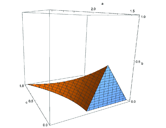
Figure 2: The set of parameters.

Obviously, for $c=0$ we get the Lozi family, $F_{a,b,0}=L_{a,b}$. Let $c\neq 0$, and fix $a$, $b$ and $c$ which satisfy the above assumptions. For simplicity, let $F:=F_{a,b,c}$. We will show that $F$ is a Lozi-like map.

Proposition 5.1.

Assume that the parameters $a,b,c$ satisfy (A1)–(A3). Then the following hold:

1. $2a+b<2(1+\sqrt{1+c^{2}})$;

2. $c<\min\{a-b-1,1\}$ and $a>b+1$;

3. If $a\geq 1$ then

   $$\frac{(a-c)(2a^{2}+3a+(2a+1)c)}{4(a+1)^{2}}\geq\frac{7}{16}a-\frac{3c^{2}+2c+2}{16};$$

4. $\displaystyle{b\leq\min\left\{\frac{(a-c)(2a^{2}+3a+(2a+1)c)}{4(a+1)^{2}},\frac{1}{2}\right\}}$;

5. $a^{3}-4a+a^{2}c-ac^{2}-c^{3}-4bc\geq(-a^{2}+2b+c^{2})\sqrt{(a+c)^{2}+4b}$.

We prove this theorem in Appendix A.

Basic properties. Let $F_{1},F_{2}:{\mathbb{R}}^{2}\to{\mathbb{R}}^{2}$ be as follows:

$$F_{1}(x,y)=(1+y+(a-c)x,bx),\ F_{2}(x,y)=(1+y-(a+c)x,bx).$$

We will first show that $F_{1}$ and $F_{2}$ are synchronously hyperbolic. Let $\Gamma$ be the $y$-axis. Then $F_{1}(\Gamma)=F_{2}(\Gamma)$ is the $x$-axis. Moreover, for every point $P\in\Gamma$, $F_{1}(P)=F_{2}(P)$. The maps $F_{1}$ and $F_{2}$ are linear and each of them maps the left half-plane onto the lower one and the right half-plane onto the upper one.

The fixed point of $F_{1}$ is $Y=\left(\frac{1}{1-a-b+c},\frac{b}{1-a-b+c}\right)$, and by (C2), it is in the third quadrant. The fixed point of $F_{2}$ is $X=\left(\frac{1}{1+a-b+c},\frac{b}{1+a-b+c}\right)$ and it is in the first quadrant. Both maps are hyperbolic. The eigenvalues of $DF_{1}$ are $\widehat{\lambda}_{1}=\frac{1}{2}\left(a-c+\sqrt{(a-c)^{2}+4b}\right)$ and $\widehat{\lambda}_{2}=\frac{1}{2}\left(a-c-\sqrt{(a-c)^{2}+4b}\right)$, and by (C2), $\widehat{\lambda}_{1}>1$ and $-1<\widehat{\lambda}_{2}<0$. The eigenvalues of $DF_{2}$ are $\lambda_{1}=\frac{1}{2}\left(-a-c-\sqrt{(a+c)^{2}+4b}\right)$ and $\lambda_{2}=\frac{1}{2}\left(-a-c+\sqrt{(a+c)^{2}+4b}\right)$, and $\lambda_{1}<-1$ and $0<\lambda_{2}<1$. The eigenvector corresponding to an eigenvalue $\lambda$ is $\langle\lambda,b\rangle$. Also, $\det DF_{i}(P)=-b$ for every point $P\in{\mathbb{R}}^{2}$ and $i=1,2$, and by (A1), $-1<\det DF_{i}(P)<0$, that is, (L1) holds.

Universal cones. The derivative of $F_{i}$, $i=1,2$, is

$$DF_{i}=\begin{bmatrix}\pm a-c&1\\ b&0\end{bmatrix},$$

where the sign depends on $i$, for $i=1$ the sign is $+$ and for $i=2$ the sign is $-$. Let

$$\begin{bmatrix}\pm a-c&1\\ b&0\end{bmatrix}\begin{bmatrix}x\\ y\end{bmatrix}=\begin{bmatrix}x^{\prime}\\ y^{\prime}\end{bmatrix}.$$

We want to find constants $0<\lambda^{\prime}<1<\lambda^{\prime\prime}$ such that $DF_{i}^{-1}$, $i=1,2$, maps the stable cone

$$K^{s}=\{\langle x^{\prime},y^{\prime}\rangle:\lambda^{\prime\prime}|x^{\prime}|\leq|y^{\prime}|\}$$

into itself and expands all its vectors by a factor larger than 1, and $DF_{i}$, $i=1,2$, maps the unstable cone

$$K^{u}=\{\langle x,y\rangle:|y|\leq\lambda^{\prime}|x|\}$$

into itself and expands all its vectors by a factor larger than 1.

Set $d=\frac{1}{2}\left(a-c-\sqrt{(a-c)^{2}-4b}\right)$. By (A1) and (A3), $(a-c)^{2}-4b>0$. By (C2), $d<b$ and consequently

$$0<d<b<1<\frac{b}{d}.$$ (5)

One can prove (see Appendix B) that

$$b|x^{\prime}|\leq d|y^{\prime}|\ \Rightarrow\ b|x|\leq d|y|,\ |x^{\prime}|\leq d|x|\ \ \textrm{and}\ \ |y^{\prime}|\leq d|y|,$$ (6)

$$|y|\leq d|x|\ \Rightarrow\ |y^{\prime}|\leq d|x^{\prime}|,\ |y^{\prime}|\geq\frac{b}{d}|y|\ \ \textrm{and}\ \ |x^{\prime}|\geq\frac{b}{d}|x|.$$ (7)

Consequently, we can take $\lambda^{\prime}=d$ and $\lambda^{\prime\prime}=b/d$. By (5) both $1/d$ and $b/d$ are larger than 1. Note that the $y$-axis is the axis of $K^{s}$ and the $x$-axis is the axis of $K^{u}$. Since $b>d^{2}$, the cones $K^{s}$ and $K^{u}$ are disjoint. Therefore, by Definition 2.3, $K^{s}$ and $K^{u}$ are the universal pair of cones. Also, by Definition 2.5, the maps $F_{1}$ and $F_{2}$ are synchronously hyperbolic.

Trapping region. We will use here notation introduced in Section 3. Let us recall that the point where $W^{u}_{F_{2}}(X)$ intersects $\Gamma$ is denoted by $D$. Let $(x_{i},y_{i}):=F^{i}(D)$. The point where $W^{s}_{F_{2}}(X)$ intersects $\Gamma$ is denoted by $M=(x_{M},y_{M})$, see Figure 3.

Calculating, we obtain

$$F(D)=\left(\frac{2+a+c+\sqrt{(a+c)^{2}+4b}}{2(1+a-b+c)},0\right),$$

$$F^{2}(D)=\left(\frac{2-2b-(a+c)\left(a+c+\sqrt{(a+c)^{2}+4b}\right)}{2(1+a-b+c)},\frac{b\left(2+a+c+\sqrt{(a+c)^{2}+4b}\right)}{2(1+a-b+c)}\right).$$

By (A1), (A3) and (C2) it follows that $x_{1}>0$, $x_{2}<0$ and $y_{2}>0$, that is, $F(D)$ belongs to the right half-plane and $F^{2}(D)$ belongs to the second quadrant. Denote by $B$ the point of intersection of the $y$-axis with the union of segments $[F(D),F^{3}(D)]\cup[F^{3}(D),F^{2}(D)]$ (remember that it may happen that $F^{3}(D)$ lies in the right half-plane). Conditions (C4) and (C5) imply (L3), that is, $[F^{3}(D),F(D)]\cap[X,M]\neq\emptyset$. Namely, (C5) implies that $F^{3}(D)$ lies to the left of the line through $X$ and $M$, and (C4) implies that $B$ is above $M$, that is, $B\in[D,M]$ (for more details see Appendices C and D). Moreover, (A3) implies (L4), that is, the stretching factor $\lambda=b/d$ is larger than $\sqrt{2}$.

Finally, let us prove (L2), that is, that there exists a trapping region $\Delta$ (for the map $F$) which is homeomorphic to an open disk and its closure is homeomorphic to a closed disk.

Let us consider the triangle $\Theta$ with vertices $F^{i}(D)$, $i=1,2,3$.

Figure 3: The triangle $\Theta$ and positions of some distinguished points.

Lemma 5.2.

Let $a$, $b$, $c$ satisfy (A1)–(A3). Then $F(\Theta)\subset\Theta$.

Proof.

Since $F$ is linear on both the left and the right half-planes, the set $F(\Theta)$ lies above the line through the points $F^{3}(D)$ and $F(D)$, and below the line through the points $F^{2}(D)$ and $F(D)$. The condition $B\in[D,M]$ implies $F(B)\in[F(M),F(D)]$. Recall that by (C5), $F^{3}(D)$ lies to the left of the line through $X$ and $M$. Therefore $F(M)$, which is the point of intersection of $[X,M]$ and $F(\Gamma)$, belongs to $\Theta$. Thus $[F(M),F(D)]\subset\Theta$.

The set $F(\Theta)$ is a pentagon with vertices $F^{i}(D)$, $i=1,2,3,4$ and $F(B)$. If $F^{4}(D)\in\Theta$, then they all belong to $\Theta$ and, consequently, $F(\Theta)\subset\Theta$. By (C2) and (C4), if $F^{3}(D)$ lies in the right half-plane, then $F^{3}(D)$ belongs to the triangle with vertices $X$, $M$, $D$, and hence $F^{4}(D)$ belongs to the triangle with vertices $X$, $F(M)$, $F(D)$ which is contained in $\Theta$. If $F^{3}(D)$ lies in the left half-plane, then (A2) implies that $F^{4}(D)$ lies to the right of the line through the points $F^{2}(D)$ and $F^{3}(D)$ (see Appendix E), and this completes the proof. ∎

Now we can define a trapping region in the same way as in [4]. We have

$$F([F^{2}(D),F^{3}(D)]\cup[F^{3}(D),F(D)]\smallsetminus\{F^{2}(D),F(D)\})\subset\mathop{\mathrm{missing}}{Int}\Theta,$$

$$F([F^{2}(D),D])=[F^{3}(D),F(D)].$$

Therefore, $F^{-4}(\Theta)$ is a neighborhood of

$$[F^{3}(D),F(D)]\cup[F^{2}(D),F^{3}(D)]\cup[F^{2}(D),D].$$

Since $[D,F(D)]$ is a local unstable manifold of the hyperbolic fixed point $X$, there exists a rectangle $R$ contained in the first quadrant, with the sides parallel to the eigenvectors of $DF(X)$, such that

$$\mathop{\mathrm{missing}}{Int}R\supset[D,F(D)]\smallsetminus F^{-4}(\mathop{\mathrm{missing}}{Int}\Theta)$$

and

$$F(R)\subset\mathop{\mathrm{missing}}{Int}R\cup F^{-4}(\mathop{\mathrm{missing}}{Int}\Theta).$$

Define $\Delta:=R\cup F^{-4}(\Theta)$. The set $\Delta$ is a compact neighborhood of $\Theta$. Let us show that it is a trapping region.

Lemma 5.3.

Let $a$, $b$, $c$ satisfy (A1)–(A3). Then $F(\Delta)\subset\mathop{\mathrm{missing}}{Int}\Delta$.

Proof.

By the definition, $F(R)\subset\mathop{\mathrm{missing}}{Int}\Delta$. Also $F^{4}(R)\supset[F(D),F^{2}(D)]\cup[F(D),F^{3}(D)]$. Therefore, $F(\Theta\smallsetminus F^{4}(R))\subset\mathop{\mathrm{missing}}{Int}\Theta$. Thus,

$$F(\Delta\smallsetminus R)=F(F^{-4}(\Theta)\smallsetminus R)=F^{-4}(F(\Theta\smallsetminus F^{4}(R)))\subset F^{-4}(\mathop{\mathrm{missing}}{Int}\Theta)\subset\mathop{\mathrm{missing}}{Int}\Delta.$$

Consequently, $F(\Delta)\subset F(R)\cup F(\Delta\smallsetminus R)\subset\mathop{\mathrm{missing}}{Int}\Delta$. ∎

Obviously, $\Delta$ is homeomorphic to a closed disk, its interior is homeomorphic to an open disk, so we have proved that $F$ satisfies (L2). Therefore, $F$ is Lozi-like.

Differences between the families $L_{a,b}$ and $F_{a,b,c}$. Recall that $L_{a,b}=F_{a,b,0}$. We want to show that the family $F_{a,b,c}$ is essentially larger than the family $L_{a,b}$. That is, we want to find parameters $a^{\prime},b^{\prime},c^{\prime}$ such that the set of kneading sequences of $F_{a^{\prime},b^{\prime},c^{\prime}}$ is different from the set of kneading sequences of any $L_{a,b}$.

We will not prove that rigorously, but we will present a very strong numerical evidence. We will comment on the reliability of our computations later.

By (C2), we have $c^{2}<a^{2}+(1-b)^{2}$, so there is a unique point $Q$ such that $Q$ is in the right half-plane, $F(Q)$ is in the left half-plane, and $F^{2}(Q)=Q$. Let us consider the maps $F_{a,b,c}$ with the following properties:

1. The point $F^{3}_{a,b,c}(D)$ lies in the left half-plane and $F^{4}_{a,b,c}(D)\in[X,M]\subset W^{s}_{F}(X)$.

2. The point $F(B)$ lies on the stable manifold of $F_{1}\circ F_{2}$ of $Q$.

Assumption (F1) means that the nonnegative part of the largest kneading sequence is $+--+^{\infty}$. Assumption (F2) means that the nonnegative part of the smallest kneading sequence is $(+-)^{\infty}$. Note that compared to Figure 3, there is a difference: $F^{4}(D)$ lies in the fourth quadrant, and $F^{5}(D)$ lies in the first quadrant (see Figure 4).

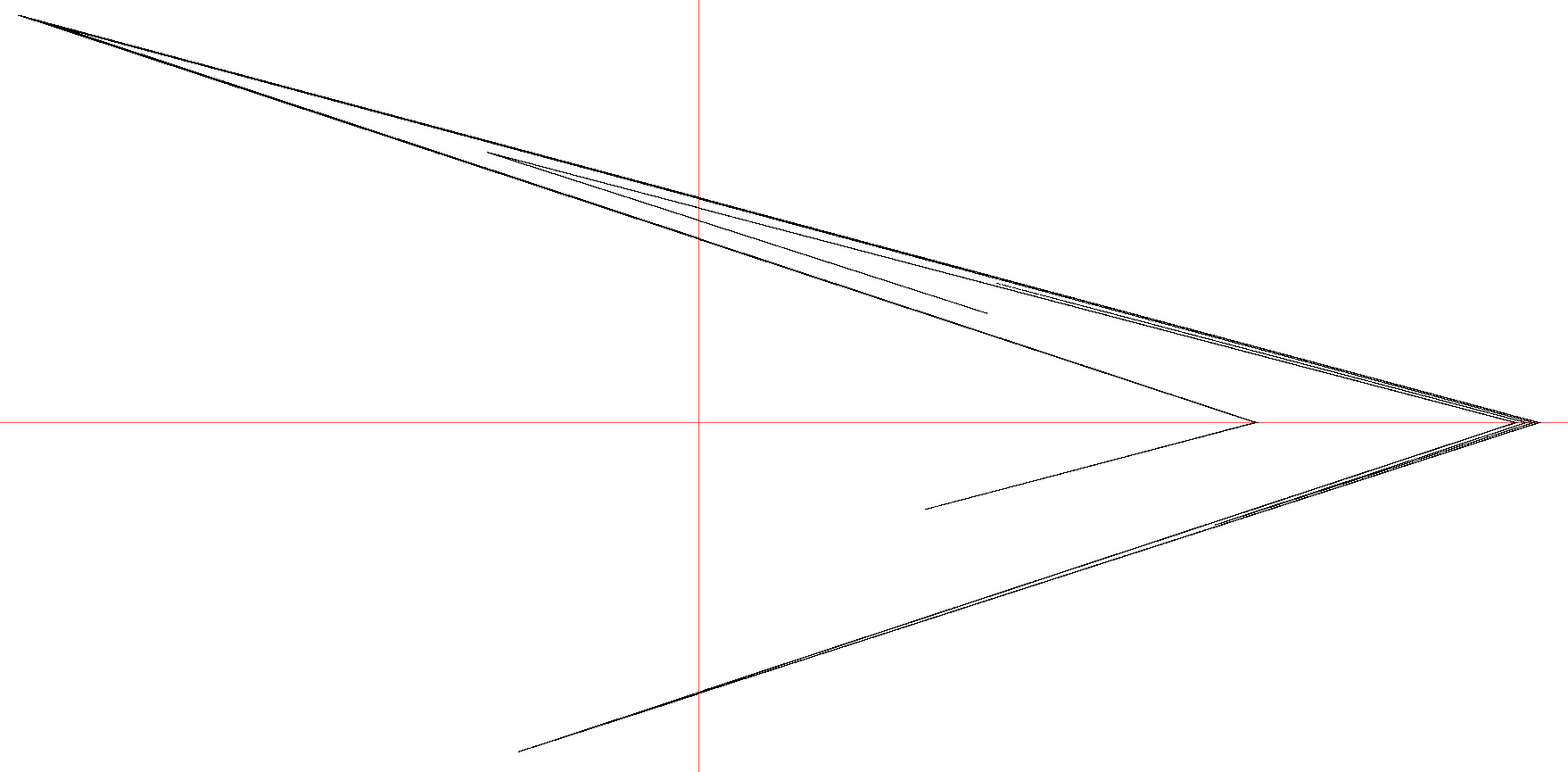
Figure 4: Attractor for the Lozi map with parameters described by (F1’) and (F2’). The $y$-coordinate is stretched by factor $7/4$.

Assumption (F1) gives the equation

$$\begin{split}(a^{2}-c^{2})^{2}-6a^{2}-4a&+4b^{2}+a^{2}b+c(2a-2ab+5bc)\\ &+(a^{3}+2a-ab+c^{3}-a^{2}c-ac^{2}+3bc)\sqrt{4b+(a+c)^{2}}=0\end{split}$$ (8)

Assumption (F2) gives the equation

$$\begin{split}-1&+\frac{1+a-b-c}{a^{2}+(-1+b)^{2}-c^{2}}+\frac{(-1+a+b+c)(a^{2}-c^{2}-\sqrt{(a^{2}-c^{2})(a^{2}-4b-c^{2})})}{2(a+c)(a^{2}+(-1+b)^{2}-c^{2})}\\ &\phantom{mmmmm}-\frac{2b}{-2b+c+\sqrt{4b+(a+c)^{2}}-a(3+2a+2c-2\sqrt{4b+(a+c)^{2}})}=0\end{split}$$ (9)

(For more details, see Appendix F.) For $c=0$ these two equations are (we simplify the second equation)

1. $a^{4}-6a^{2}-4a+4b^{2}+a^{2}b+(a^{3}+2a-ab)\sqrt{4b+a^{2}}=0$,

2. $\displaystyle{4\cdot\frac{-a^{2}-2b^{2}+2b+a\sqrt{a^{2}-4b}}{a-2b-\sqrt{a^{2}-4b}}-\left(2+a-\sqrt{a^{2}+4b}\right)\left(3a-\sqrt{a^{2}+4b}\right)=0}.$

Computer plots of the graphs of the above equations are presented in Figure 5. The graphs are smooth and evidently intersect each other at one point (although we cannot claim that we proved it). Moreover, using the “NSolve” command of Wolfram Mathematica produces a unique solution to this system of equations in the region $a\in[1,2]$, $b\in[0,1]$. This solution is approximately

$$a=1.65531960296885174459210852526,\ \ \ b=0.276507107967726099812119447619.$$

The problem is that we do not know how the computer produces graphs or solves a system of equations. Thus, it could happen that the graphs have more branches. To eliminate this possibility, we checked for both (F1’) and (F2’) whether the left-hand side is positive or negative (in the region mentioned above), see Figure 6. This method would identify (although with limited precision) additional solutions. However, it gave us the same result as before.

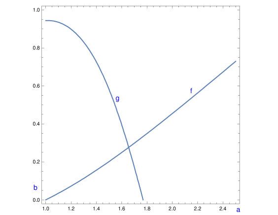
Figure 5: Graphs of (F1’) and (F2’).

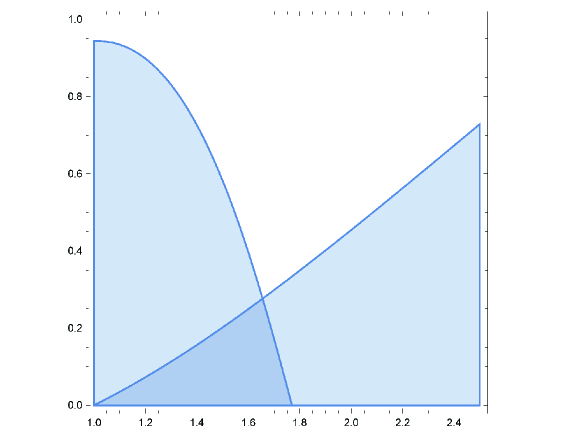
Figure 6: Equations (F1’) and (F2’) as inequalities.

For $c=0.1$ the values of $a$ and $b$ are approximately

$$a=1.63537454884191587958622457986,\ \ \ b=0.276988367360779957370639853557.$$

Here we do not have to worry about the uniqueness. We just need some values of parameters. One can check that in both cases, $c=0$ and $c=0.1$, the map satisfies conditions (A1)–(A3).

We computed kneading sequences using Free Pascal. Re-checking numerically nonnegative parts of the largest and smallest kneading sequences in both cases, we get correct signs for at least 68 iterates. Since the maximal stretching factor of $F$ is about $1.8$, and the precision of our floating point computations is about 19 decimal places, this is what we could expect.

Now we look at the nonnegative parts of the kneading sequence of the turning point $S$ which is the next after $F(D)$ along the unstable manifold of $X$ in that direction (of course, $S$ depends on $c$). In Figure 4, this turning point is the leftmost of the right group of turning points. For $c=0$, the nonnegative part of the kneading sequence starts with $+--+++-+-+-+++-++$, while for $c=0.1$ it starts with $+--+++-+-+-+++++-$. We see a difference at the place corresponding to $F^{14}(S)$. The distance of this point from the divider is about $0.6$ for $c=0$ and about $8\cdot 10^{-4}$ for $c=0.1$ (if one wants much larger distances, they appear for $F^{16}(S)$). The roundoff error, even if we take into account accumulation of errors, should not be larger than $10^{-14}$, so the results are quite reliable.

Remark 5.4.

Note that even for the case $c=0$ (that is, for the Lozi maps) (C4) and (C5) imply (L3). In [4], (L3) was obtained by a stronger condition, $b<(a^{2}-1)/(2a+1)$. By replacing this condition by our part of (C4), $b\leq\frac{(a-c)(2a^{2}+3a+(2a+1)c)}{4(a+1)^{2}}$, we get a slightly larger region in the parameter plane for the Lozi family, where the hyperbolic attractor exists. This new region is the triangle bounded by the lines $b=0$, $2a+b=4$, and $a\sqrt{2}=b+2$, according to (A1)–(A3). The gain is a small region close to the top of this triangle, that was cut off in [4].

Remark 5.5.

Although we were concerned only with the nonnegative parts of the kneading sequences, it is clear that the whole largest (respectively, smallest) kneading sequences are the same for the cases $c=0$ and $c=0.1$.

Appendix

A Proof of Theorem 5.1

(C1) Suppose that $2a+b\geq 2(1+\sqrt{1+c^{2}})$. Then, by (A2), $2(1+\sqrt{1+c^{2}})(1-\frac{c^{2}}{(a+b)^{2}})<4$, and hence, $\frac{c^{2}}{(a+b)^{2}}>1-\frac{2}{1+\sqrt{1+c^{2}}}=\frac{c^{2}}{(1+\sqrt{1+c^{2}})^{2}}$. Therefore, $a+b<1+\sqrt{1+c^{2}}$. Then $2(1+\sqrt{1+c^{2}})\leq 2a+b<a+(1+\sqrt{1+c^{2}})$, so $a>1+\sqrt{1+c^{2}}$, and hence $1+\sqrt{1+c^{2}}<a<a+b<1+\sqrt{1+c^{2}}$, a contradiction.

(C2) Since $0<b<1$, we have $-\frac{b+2}{\sqrt{2}}<-b-1$, so $c<a-\frac{b+2}{\sqrt{2}}<a-b-1$. In particular, $a-b-1>0$. Now we will prove that $c<1$. By (C1), $2a<2+2\sqrt{1+c^{2}}-b$. By (A3), $2a>2c+\sqrt{2}b+2\sqrt{2}$. Thus, $2c+\sqrt{2}b+2\sqrt{2}<2+2\sqrt{1+c^{2}}-b$, so $0<(\sqrt{2}+1)b<2(1+\sqrt{1+c^{2}}-c-\sqrt{2})$. Set $\varphi(c)=1+\sqrt{1+c^{2}}-c-\sqrt{2}$. Then $\varphi(1)=0$ and $\varphi^{\prime}(c)=\frac{c}{\sqrt{1+c^{2}}}-1<0$. Thus, $c<1$.

(C3) We have

$$\frac{(a-c)(2a^{2}+3a+(2a+1)c)}{4(a+1)^{2}}=\frac{a}{2}-\frac{1}{4}-\frac{2ac+(2a+1)c^{2}-1}{4(a+1)^{2}}.$$

Thus, we only need to prove that if $a\geq 1$ then

$$\frac{2ac+(2a+1)c^{2}-1}{4(a+1)^{2}}\leq\frac{3c^{2}+2c+2}{16}-\frac{1}{4}+\frac{a}{16}.$$ (10)

If $a=1$, (10) is an equality. The derivative with respect to $a$ of the left-hand side is

$$\frac{-ac^{2}-ac+c+1}{2(a+1)^{3}}\leq\frac{1}{2(a+1)^{3}}\leq\frac{1}{16}$$

if $a\geq 1$, while the derivative of the right-hand side is $\frac{1}{16}$. Thus, the inequality (10) holds.

(C4) We know by (A3) that

$$\sqrt{2}a-b>\sqrt{2}c+2.$$ (11)

Also, by (C1), $2a+b<2\left(1+\sqrt{1+c^{2}}\right)$. However, $\sqrt{1+c^{2}}\leq 1+c$, so

$$2a+b<4+2c.$$ (12)

By (C3), to prove that $b\leq\frac{(a-c)(2a^{2}+3a+(2a+1)c)}{4(a+1)^{2}}$, we only need to prove that

$$b<\frac{7}{16}a-\frac{3c^{2}+2c+2}{16}.$$ (13)

Consider three lines in the $(a,b)$-plane given by equalities in (11), (12) and (13). Taking into account the slopes of those lines, we see that if $(a_{0},b_{0})$ is the point of intersection of two first lines, it is enough to prove that (13) holds for $a=a_{0}$, $b=b_{0}$. We have $a_{0}=\frac{6}{2+\sqrt{2}}+c$ and $b_{0}=4-\frac{12}{2+\sqrt{2}}<\frac{1}{2}$, so, in particular, $b<\frac{1}{2}$. Hence, it is enough to prove that $\frac{1}{2}<\frac{7}{16}\left(\frac{6}{2+\sqrt{2}}+c\right)-\frac{3c^{2}+2c+2}{16}$, that is $\frac{42}{2+\sqrt{2}}-10+5c-3c^{2}>0$. However, $\frac{42}{2+\sqrt{2}}>10$, and, by (C2), $5c>3c^{2}$.

(C5) By (A3), $a>\sqrt{2}$, so $a^{2}>2$. By (C4), $b<\frac{1}{2}$, so $2b<1$. By (C2) and (A1), $0\leq c<1$, so $c^{2}<1$. Thus, $-a^{2}+2b+c^{2}<0$. Therefore, $(-a^{2}+2b+c^{2})\sqrt{(a+c)^{2}+4b}<(-a^{2}+2b+c^{2})(a+c)$, so if

$$a^{3}-4a+(a^{2}-4b)c-ac^{2}-c^{3}\geq(-a^{2}+2b+c^{2})(a+c),$$ (14)

then (C5) holds. Thus, we will be proving (14).

By (A3), $b<(a-c)\sqrt{2}-2=:b_{1}$. If (14) holds for $b=b_{1}$, then replacing $b_{1}$ by $b$ in (14) will make the left-hand side larger and the right-hand side smaller, so (14) still holds. Therefore, it is enough to prove (14) for $b=b_{1}$, that is

$$a^{3}+(c-\sqrt{2})a^{2}+(-c^{2}-2\sqrt{2}c)a+(-c^{3}+3\sqrt{2}c^{2}+6c)\geq 0.$$ (15)

The derivative of the left-hand side of (15) with respect to $a$ is

$$3a^{2}+2(c-\sqrt{2})a+(-c^{2}-2\sqrt{2}c)=(a+c)(3a-c-2\sqrt{2}).$$

Since $a\geq\sqrt{2}$, we have $3a-c-2\sqrt{2}\geq 3\sqrt{2}-1-2\sqrt{2}>0$. Therefore, the left-hand side of (15) increases with $a$. Thus, it is enough to check (15) for $a=\sqrt{2}$:

$$2\sqrt{2}+2(c-\sqrt{2})+\sqrt{2}(-c^{2}-2\sqrt{2}c)+(-c^{3}+3\sqrt{2}c^{2}+6c)=4c+c^{2}(2\sqrt{2}-c)>0.$$

B Existence of universal cones

Both $d$ and $b/d$ are roots of the equation $\lambda^{2}-(a-c)\lambda+b=0$, so in particular, $d+b/d=a-c$.

In order to prove (6), we may assume that $y^{\prime}=1$ and $|x^{\prime}|\leq d/b$. Then $x=1/b$ and $y=x^{\prime}-\frac{\pm a-c}{b}$, and we have to prove that

$$1\leq d\left|x^{\prime}-\frac{\pm a-c}{b}\right|,\ \ \frac{d}{b}\leq d\cdot\frac{1}{b},\ \ 1\leq d\left|x^{\prime}-\frac{\pm a-c}{b}\right|.$$ (16)

The second inequality holds and the first and third are identical. We have

$$\left|x^{\prime}-\frac{\pm a-c}{b}\right|\geq\frac{a-c}{b}=|x^{\prime}|\geq\frac{a-c}{b}-\frac{d}{b}=\frac{b}{db}=\frac{1}{d},$$

so (16) holds.

Similarly, in order to prove (7), we may assume that $x=1$ and $|y|\leq d$. Then $x^{\prime}=\pm a-c+y$ and $y^{\prime}=b$, and we have to prove that

$$b\leq d|\pm a-c+y|,\ \ b\geq\frac{b}{d}\cdot d,\ \ |\pm a-c+y|\geq\frac{b}{d}.$$ (17)

Again, the second inequality holds and the first and third are equivalent. We have

$$|\pm a-c+y|\geq a-c-d=\frac{b}{d},$$

so (17) holds.

C $F^{3}(D)$ lies to the left of the line through $X$ and $M$

There are several ways to find a condition which implies that $F^{3}(D)$ lies to the left of the line through $X$ and $M$. The simplest condition is $y_{3}-y_{Q}>0$, where $Q=(x_{Q},y_{Q})$ denotes the point on the line through $X$ and $M$ such that $x_{Q}=x_{3}$. Calculation shows that $y_{Q}=sx_{3}+y_{M}$, where

$$s=\frac{2b}{-a-c+\sqrt{4b+(a+c)^{2}}}$$

is the slope of the line through $X$ and $M$, and

$$y_{M}=\frac{b}{1+a-b+c}-\frac{2b}{(1+a-b+c)(-a-c+\sqrt{4b+(a+c)^{2}})}.$$

Now the inequality $y_{3}-y_{Q}>0$ follows from (C5).

D $B$ is above $M$

If $F^{3}(D)$ lies in the right half-plane, then $B\in[F^{3}(D),F^{2}(D)]$ and by Appendix C, $B$ is above $M$. If $F^{3}(D)$ lies in the left half-plane, then $B\in[F(D),F^{3}(D)]$. Let $N=(x_{N},y_{N})$ denote the point of intersection of $[X,M]$ and $[F(D),F^{3}(D)]$. Then $B$ being above $M$ is equivalent to $x_{N}>0$. Calculation shows that $x_{N}=y_{M}+s_{13}x_{1}/(s_{13}-s)$, where

$$s_{13}=\frac{b(3a-c+\sqrt{4b+(a+c)^{2}})}{-2b+4a(a-c)}$$

is the slope of the line through $F(D)$ and $F^{3}(D)$. Now the inequality $x_{N}>0$ follows from (C4).

E $F^{4}(D)$ lies to the right of the line through $F^{2}(D)$ and $F^{3}(D)$

A condition which implies that $F^{4}(D)$ lies to the right of the line through $F^{2}(D)$ and $F^{3}(D)$ is $x_{4}-x_{P}>0$, where $P=(x_{P},y_{P})$ denotes the point on the line through $F^{2}(D)$ and $F^{3}(D)$ such that $y_{P}=y_{4}$. Calculation shows that $y_{P}=x_{2}+(y_{4}-y_{2})/s_{23}$, where

$$s_{23}=\frac{2b^{2}}{2a^{2}+a\left(3b+2c-2\sqrt{4b+(a+c)^{2}}\right)-b\left(c+\sqrt{4b+(a+c)^{2}}\right)}$$

is the slope of the line through $F^{2}(D)$ and $F^{3}(D)$. Now the inequality $x_{4}-x_{P}>0$ follows from (A2).

F Differences between the families $L_{a,b}$ and $F_{a,b,c}$

Condition $F^{4}_{a,b,c}(D)\in[X,M]$ is equivalent to the equality $y_{4}-y_{X}-s(x_{4}-x_{X})=0$ (where $X=(x_{X},y_{X})$), and gives the equation (8).

For the assumption (F2), note first that $Q$ has coordinates

$$Q=(x_{Q},y_{Q})=\left(\frac{1+a-b-c}{a^{2}+(-1+b)^{2}-c^{2}},-\frac{b(-1+a+b+c)}{a^{2}+(-1+b)^{2}-c^{2}}\right),$$

and the stable manifold of $F_{1}\circ F_{2}$ of $Q$ has slope

$$s_{2}=\frac{2b(a+c)}{a^{2}-c^{2}-\sqrt{-4b^{2}+(a^{2}-2b-c^{2})^{2}}}.$$

Also,

$$F(B)=(x_{B_{1}},y_{B_{1}})=\left(1-\frac{b(3a-c+\sqrt{4b+(a+c)^{2}})(2+a+c+\sqrt{4b+(a+c)^{2}})}{2(-2b+4a(a-c))(1+a-b+c)},0\right).$$

The condition that $F(B)$ lies on the stable manifold of $F_{1}\circ F_{2}$ of $Q$ is equivalent to the equality $y_{Q}-s_{2}(x_{Q}-x_{B_{1}})=0$ and gives the equation (9).

Michał Misiurewicz
Department of Mathematical Sciences
Indiana University – Purdue University Indianapolis
402 N. Blackford Street, Indianapolis, IN 46202
mmisiure@math.iupui.edu
http://www.math.iupui.edu/$\sim$mmisiure

Sonja Štimac
Department of Mathematics
Faculty of Science, University of Zagreb
Bijenička 30, 10 000 Zagreb, Croatia
sonja@math.hr
http://www.math.hr/$\sim$sonja

References

- [1] M. Brin, G. Stuck, Introduction to Dynamical Systems, Cambridge University Press (2002).
- [2] Y. Ishii, Towards a kneading theory for Lozi mappings I. A solution of the pruning front conjecture and the first tangency problem, Nonlinearity 10 (1997), no. 3, 731–747.
- [3] R. Lozi, Un attracteur etrange(?) du type attracteur de Hénon, J. Physique (Paris) 39 (Coll. C5) (1978), no. 8, 9–10.
- [4] M. Misiurewicz, Strange attractor for the Lozi mappings, Ann. New York Acad. Sci. 357 (1980) (Nonlinear Dynamics), 348–358.
- [5] M. Misiurewicz, S. Štimac, Symbolic dynamics for Lozi maps, Nonlinearity 29 (2016), no. 10, 3031–3046.