Light-quarks Yukawa couplings and new physics in exclusive high-$p_{T}$ Higgs + jet and Higgs + $b$-jet events

Abstract

We suggest that the exclusive Higgs + light (or b)-jet production at the LHC, $pp\to h+j(j_{b})$, is a rather sensitive probe of the light-quarks Yukawa couplings and of other forms of new physics (NP) in the Higgs-gluon $hgg$ and quark-gluon $qqg$ interactions. We study the Higgs $p_{T}$-distribution in $pp\to h+j(j_{b})\to\gamma\gamma+j(j_{b})$, i.e., in $h+j(j_{b})$ production followed by the Higgs decay $h\to\gamma\gamma$, employing the ($p_{T}$-dependent) signal strength formalism to probe various types of NP which are relevant to these processes and which we parameterize either as scaled Standard Model (SM) couplings (the kappa-framework) and/or through new higher dimensional effective operators (the SMEFT framework). We find that the exclusive $h+j(j_{b})$ production at the 13 TeV LHC is sensitive to various NP scenarios, with typical scales ranging from a few TeV to ${\cal O}(10)$ TeV, depending on the flavor, chirality and Lorentz structure of the underlying physics.

I Introduction

The next runs of the LHC will be dedicated to two primary tasks: the search for new physics (NP) and the detailed scrutiny of the Higgs properties, which might shed light on NP specifically related to the origin of mass and flavor and to the observed hierarchy between the two disparate Planck and ElectroWeak (EW) scales. Indeed, the study of Higgs systems is in particular challenging, since it requires precision examination of some of its weakest couplings (within the SM) and measurements of highly non-trivial processes involving high jet multiplicities, large backgrounds and low detection efficiencies.

The s-channel Higgs production and its subsequent decays, $pp\to h\to ff$, which led to its discovery, are relatively inefficient for NP searches. In particular, if the NP scale, $\Lambda$, is of ${\cal O}({\rm TeV})$ and larger, then its effect in these processes is expected to be suppressed by at least $\sim m_{h}^{2}/\Lambda^{2}$, since most of these events come from the dominant gluon fusion s-channel production mechanism and are, therefore, clustered around $\sqrt{s}\simeq m_{h}$. However, in some fraction of the events, the Higgs recoils against one or more hard jets and, thus, carries a large $p_{T}$, which may play a key role in the hunt for NP and/or for background rejection in Higgs studies. Indeed, a key observable for Higgs boson events is the number of jets produced in the event. For that reason, and since the Higgs $p_{T}$ distribution is sensitive to the production mechanism, there has recently been a growing interest, both experimentally ATLAS1 ; ATLAS2 ; ATLAS3 ; ATLAS4 ; CMS1 ; CMS2 and theoretically hjth1 ; schulz2 ; schulz3 ; hjth2 ; hjth3 ; hjth4 ; hjth5 ; highptrecent ; 1703.03886 , in the behavior of the Higgs $p_{T}$ distribution in inclusive and exclusive Higgs production, where the Higgs carries a substantial fraction of transverse momentum (for earlier work see veryearly1 ; veryearly2 ; early1 ; early2 ). In particular, the Higgs $p_{T}$ distribution in the exclusive Higgs + jets production, $pp\to h+nj$, was one of the prime targets of the measurements performed recently by ATLAS and CMS ATLAS1 ; ATLAS2 ; ATLAS3 ; ATLAS4 ; CMS1 ; CMS2 .

In this paper we will thus focus on the exclusive Higgs + 1-jet production, $pp\to h+j$, where $j$ stands for either a “light-jet” defined as any non-flavor tagged jet originating from a gluon or light-quarks $j=g,u,d,c,s$ (i.e., assuming them to be indistinguishable from the observational point of view) or a $b$-quark jet ($j_{b}$). It is interesting to note that there has been some hints in the LHC 8 TeV data for an excess in the $h+j$ channel ATLAS3 ; schulz3 , although the statistics are still limited and the theoretical uncertainties are relatively large. Indeed, a significant effort has been dedicated in recent years, from the theory side, towards understanding and reducing the uncertainties pertaining to the Higgs+jet production cross-section at the LHC hjth1 ; schulz1 ; schulz2 ; hjth2 ; hjth3 ; hjth4 ; hjth5 ; hbjet1 ; 1704.06620 , with special attention given to higher transverse momentum of the Higgs, where NP effects are expected to become more apparent. In particular, the high-$p_{T}$ Higgs spectrum in $pp\to h+j(j_{b})$ can be sensitive to various well motivated NP scenarios, such as supersymmetry susyhj ; 0309204 ; dawson1 ; dawson2 , heavy top-partners toppartner , higher dimensional effective operators 1312.3317_SMEFT ; 1411.2029 ; 1409.6299_dawson ; 1308.2225_dim7 ; hbjet2_bMM and NP in Higgs-top quark and Higgs-gluon interactions in the so-called “kappa-framework”, where one assumes that the $hgg$ and $htt$ interactions are scaled by some factor with respect to the SM 1309.5273 ; 1405.4295 ; 1405.7651 ; 1612.00283 .

In general, there is a tree-level contribution to $pp\to h+j(j_{b})$ in the SM from the hard processes $gq\to qh,~{}g\bar{q}\to\bar{q}h$ and $q\bar{q}\to gh$ ($q=u,d,c,s,b$). The corresponding SM tree-level diagrams, which are depicted in Fig. 1, are proportional to the light-quarks Yukawa couplings, $y_{q}$, so that the SM tree-level contribution to the overall $pp\to h+j(j_{b})$ cross-section is small (e.g., in the case of $pp\to h+c$, it is at the percent level). In particular, the squared matrix elements, summed and averaged over spins and colors, for these tree-level hard processes are:

$$\sum\overline{\left|{\cal M}_{SM}^{q\bar{q}\to gh}\right|^{2}} = \frac{2g_{s}^{2}y_{q}^{2}}{{\cal C}_{qq}}\frac{m_{h}^{4}+\hat{s}^{2}}{\hat{t}\hat{u}}~{},$$ (1)

$$\sum\overline{\left|{\cal M}_{SM}^{qg\to qh}\right|^{2}} = -\frac{{\cal C}_{qq}}{{\cal C}_{qg}}\sum\overline{\left|{\cal M}_{SM}^{q\bar{q}\to gh}\right|^{2}}(\hat{s}\leftrightarrow\hat{t})~{},$$ (2)

$$\sum\overline{\left|{\cal M}_{SM}^{\bar{q}g\to\bar{q}h}\right|^{2}} = -\frac{{\cal C}_{qq}}{{\cal C}_{qg}}\sum\overline{\left|{\cal M}_{SM}^{q\bar{q}\to gh}\right|^{2}}(\hat{s}\leftrightarrow\hat{u})~{},$$ (3)

where $\hat{s}=(p_{1}+p_{2})^{2},~{}\hat{t}=(p_{1}+p_{3})^{2}$ and $\hat{u}=(p_{2}+p_{3})^{2}$, defined for the process $q(-p_{1})+\bar{q}(-p_{2})\to h+g(p_{3})$. Also, $g_{s}$ is the strong coupling constant and ${\cal C}_{qq}=N^{2}$, ${\cal C}_{qg}=NV$ are the color average factors, where $V=N^{2}-1=8$ corresponds to the number of gluons in the adjoint representation of the SU(N) color group.

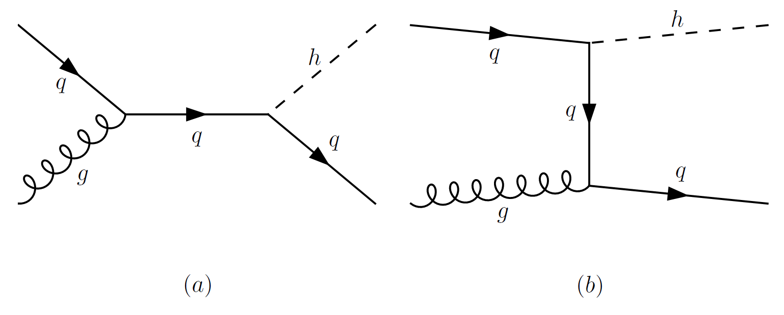
Figure 1: The tree-level SM diagrams for $gq\to qh$, where $q=u,d,c,s,b$. The diagrams corresponding to $g\bar{q}\to h\bar{q}$ and $q\bar{q}\to gh$ can be obtained by crossing symmetry, see also text.

Thus, in the limit $y_{q}\to 0$, the dominant and leading order (LO) SM contribution to the Higgs + light-jet cross-section, $\sigma(pp\to h+j)$, arises from the 1-loop process $gg\to gh$, which is generated by 1-loop top-quark exchanges (and the subdominant b-quark loops bquark-loops ), and can be parameterized by an effective Higgs-gluon $ggh$ interaction Lagrangian:

$${\cal L}_{eff}^{ggh}=C_{g}hG_{\mu\nu}^{a}G^{\mu\nu,a}~{},$$ (4)

where $C_{g}$ is the Higgs-gluon point-like effective coupling, which at lowest order in the SM is veryearly1 ; veryearly2 : $C_{g}=\alpha_{s}/(12\pi v)$, where $v=246$ GeV is the Higgs vacuum expectation value (VEV). In what follows we will use the point-like $ggh$ effective coupling of Eq. 4 with $C_{g}$ given as an asymptotic expansion in $1/m_{t}$ up to $m_{t}^{-6}$, as implemented in MADGRAPH5 for the Higgs effective field theory (HEFT) model HEFTggh . We will neglect throughout this work the 1-loop effects of the b-quark and of the lighter quarks with enhanced Yukawa couplings (i.e., as large as the b-quark Yukawa), which are expected to yield a correction at the level of a few percent compared to the dominant top-quark loops, when the Higgs transverse momentum is larger than $\sim m_{h}/2$ bquark-loops ; 1606.09253 .

This prescription for the Higgs-gluon coupling is a good approximation for a Higgs produced with a $p_{T}(h)\>\raisebox{-2.15277pt}{$\stackrel{{\scriptstyle\textstyle<}}{{\sim}}$}\>200$ GeV, see e.g., highptrecent ; overestimate , whereas, as will be shown in this work, the harder $p_{T}(h)\>\raisebox{-2.15277pt}{$\stackrel{{\scriptstyle\textstyle>}}{{\sim}}$}\>200$ GeV regime is important for probing NP in Higgs +jet production. However, since the exact form of the loop induced $ggh$ interaction (i.e., using a finite top-quark mass) is currently unknown beyond LO (1-loop), we choose to work with the effective $ggh$ point-like interaction (as described above) in order to simplify the calculation and the presentation of our analysis. Given the exploratory nature of this work and the type of study presented, this approximation is not expected to have an effect on our results at a level which changes the main outcome and conclusions of this work. In particular, in order to give an estimate of the sensitivity of our results to the calculation scheme, we will also study and analyse some samples of our results using the exact LO calculation of the 1-loop diagrams (mass dependent top-quark exchanges) which involve the $ggh$ interaction vertex. Indeed, since this LO 1-loop calculation is the only currently available exact (mass dependent) calculational setup for $pp\to h+j(j_{b})$, a comparison between the NP effects calculated with the point-like $ggh$ approximation and with the mass dependent 1-loop diagrams can serve as a yardstick for the uncertainty and sensitivity of our results to the calculational setup.

The subprocesses $gq\to qh$, $g\bar{q}\to\bar{q}h$ and $q\bar{q}\to gh$ (which, as can be seen from Eqs. 1-3, are proportional to $y_{q}^{2}$ at tree-level) also receive a 1-loop contribution from the above $ggh$ effective vertex (i.e., from the top-quark loops), which is, however, small compared to the $gg\to gh$ veryearly1 ; veryearly2 ; early1 ; early2 . In particular, the $gg\to gh$ contribution to $\sigma(pp\to h+j)$ at the LHC is about an order of magnitude larger than the one from $gq\to qh$ and more than two orders of magnitude larger than the two other channels $g\bar{q}\to\bar{q}h$ and $q\bar{q}\to gh$.

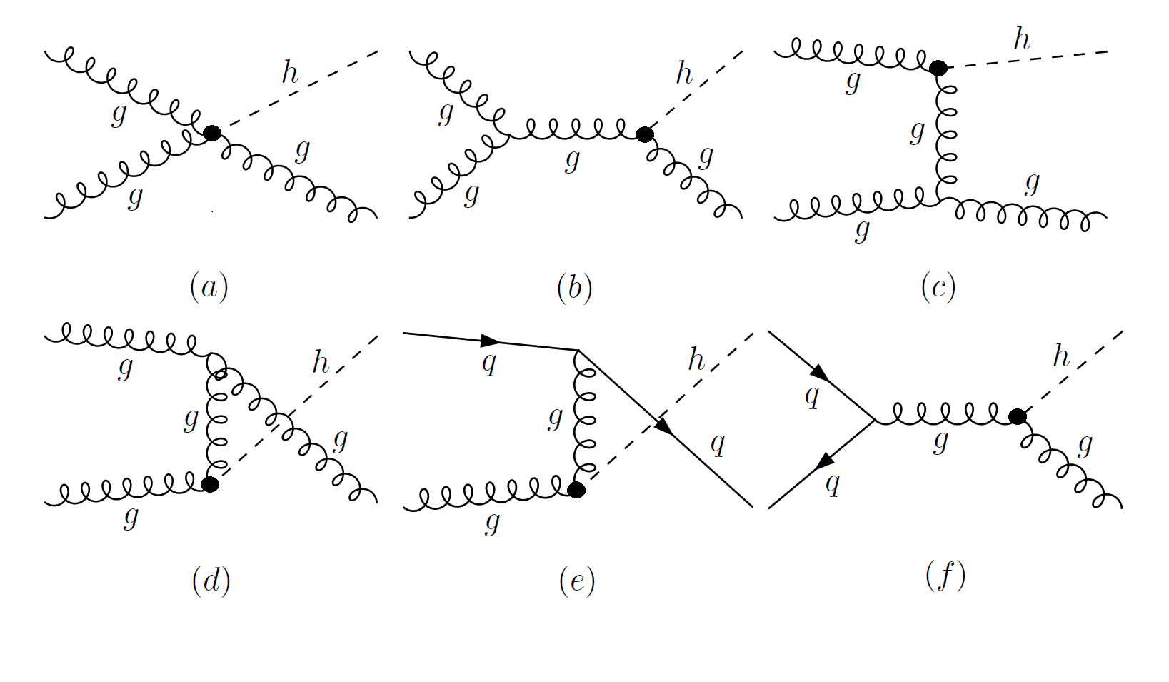
Figure 2: The 1-loop SM diagrams for $gg\to gh,~{}gq\to qh$ and $q\bar{q}\to gh$, in the effective Higgs-gluon description, where the loop-induced $ggh$ and $gggh$ vertices are represented by a heavy dot. See also text.

The 1-loop (and LO for $y_{q}=0$) SM differential hard cross-sections for $gg\to gh,~{}gq\to qh,g\bar{q}\to\bar{q}h$ and $q\bar{q}\to gh$ (the corresponding SM diagrams for all channels are shown in Fig. 2), expressed in terms of the above effective $ggh$ interaction and neglecting the light-quark masses, are given by veryearly1 ; veryearly2 :

$$\sum\overline{\left|{\cal M}_{SM}^{gg\to gh}\right|^{2}} \simeq \frac{96g_{s}^{2}C_{g}^{2}}{{\cal C}_{gg}}\frac{m_{h}^{8}+\hat{s}^{4}+\hat{t}^{2}+\hat{u}^{2}}{\hat{s}\hat{t}\hat{u}}~{},$$ (5)

$$\sum\overline{\left|{\cal M}_{SM}^{q\bar{q}\to gh}\right|^{2}} \simeq \frac{16g_{s}^{2}C_{g}^{2}}{{\cal C}_{qq}}\frac{\hat{t}^{2}+\hat{u}^{2}}{\hat{s}}~{},$$ (6)

$$\sum\overline{\left|{\cal M}_{SM}^{qg\to qh}\right|^{2}} \simeq -\frac{{\cal C}_{qq}}{{\cal C}_{qg}}\sum\overline{\left|{\cal M}_{SM}^{q\bar{q}\to gh}\right|^{2}}(\hat{s}\leftrightarrow\hat{t})~{},$$ (7)

$$\sum\overline{\left|{\cal M}_{SM}^{\bar{q}g\to\bar{q}h}\right|^{2}} \simeq -\frac{{\cal C}_{qq}}{{\cal C}_{qg}}\sum\overline{\left|{\cal M}_{SM}^{q\bar{q}\to gh}\right|^{2}}(\hat{s}\leftrightarrow\hat{u})~{},$$ (8)

where ${\cal C}_{gg}=V^{2}=64$ and $\hat{s}=(p_{1}+p_{2})^{2},~{}\hat{t}=(p_{1}+p_{3})^{2},~{}\hat{u}=(p_{2}+p_{3})^{2}$, with momenta defined via $h\to g(p_{1})+g(p_{2})+g(p_{3})$ for $gg\to gh$ and via $q(-p_{1})+\bar{q}(-p_{2})\to h+g(p_{3})$ for $q\bar{q}\to gh$.

Turning now to the possible manifestation of NP in Higgs + jet production at the LHC, there are, in principle, two ways in which $pp\to h+j(j_{b})$ can be modified:

• when the NP generates new interactions that are absent in the SM and that can potentially change the SM kinematic distributions in this process.

• when the NP comes in the form of scaled SM couplings, corresponding to the previously mentioned kappa-framework.

We will explore both types of NP effects in $pp\to h+j$ and $pp\to h+j_{b}$ and, in particular, focus on NP that modifies the light and b-quarks Yukawa couplings and/or the light and b-quarks interactions with the gluon, as well as the Higgs-gluon effective vertex in Eq. 4. Indeed, the Higgs mechanism of the SM implies that the fermion’s Yukawa couplings are proportional to the ratio between their masses and the EW VEV, i.e., $y_{f}\propto m_{f}/v$. Thus, at least for the light fermions of the 1st and 2nd generations [where $m_{f}/v\sim{\cal O}(10^{-5})$ and $m_{f}/v\sim{\cal O}(10^{-4}-10^{-3})$, respectively], any signal which can be associated with their Yukawa couplings would stand out as clear evidence for NP beyond the SM. The current experimental bounds on the Yukawa couplings of light-quark’s of the 1st and 2nd generations, $y_{u},y_{d},y_{s},y_{c}$, coming from fits to the measured Higgs data, allow them to be as large as the b-quark Yukawa $y_{b}$ bounds1 . From the phenomenological point of view, it is, therefore, important to explore the possibility that the light-quark Yukawa couplings and/or their interactions with the gauge boson’s are significantly enhanced or modified with respect to the SM. Indeed, there has recently been a growing interest in the study of light-quark’s Yukawa couplings, see e.g., perez1 ; yotam1 ; 1606.09253 ; 1608.04376 ; felix ; han ; 1608.01746 ; 1405.0990 ; han1 . For example, in yotam1 ; 1606.09253 , the Higgs $p_{T}$ distributions in inclusive Higgs production, $pp\to h+X$, was used to study the sensitivity to $y_{q}$, where it was shown that the measurements from the 8 TeV LHC run constrain the Yukawa couplings of the 1st generation quarks and the c-quark to be $y_{u},y_{d}\>\raisebox{-2.15277pt}{$\stackrel{{\scriptstyle\textstyle<}}{{\sim}}$}\>0.5y_{b}$ yotam1 and $y_{c}\>\raisebox{-2.15277pt}{$\stackrel{{\scriptstyle\textstyle<}}{{\sim}}$}\>5y_{b}$ 1606.09253 , respectively. Slightly improved bounds are expected in the inclusive channel at the future LHC Runs: $y_{u},y_{d}\>\raisebox{-2.15277pt}{$\stackrel{{\scriptstyle\textstyle<}}{{\sim}}$}\>0.3y_{b}$ yotam1 ; 1608.04376 and $y_{c}\>\raisebox{-2.15277pt}{$\stackrel{{\scriptstyle\textstyle<}}{{\sim}}$}\>y_{b}$ 1606.09253 . As we will see below, a $p_{T}$-dependent ratio between the NP and SM cross-sections (the signal strength) for the exclusive Higgs + jet production cross-section, $\sigma(pp\to h+j)$, followed by the Higgs decays to e.g., $\gamma\gamma$ and $WW^{\star}$, may be used to put comparable and, in some cases, stronger constraints on $y_{q}$. In particular, we will show that, if the $ggh$ effective coupling also deviates from its SM value, then significantly stronger bounds on $y_{q}$ are expected.

We also explore exclusive Higgs + jet production in the SMEFT, defined as the expansion of the SM Lagrangian with an infinite series of higher dimensional effective operators. We find that the exclusive $pp\to h+j(j_{b})$ signal can probe the NP scenarios portrayed by the SMEFT with typical scales ranging from a few to ${\cal O}(10)$ TeV, depending on the details of underlying physics.

The paper is organized as follows: in section II we outline our notation and define our observables for the study of NP in $pp\to h+j$ and $pp\to h+j_{b}$. In sections III and IV we discuss the NP effects in $pp\to h+j(j_{b})$ within the kappa and the SMEFT frameworks, respectively, and in section V we summarize.

II Notation and observables

We define the signal strength for $pp\to h+j$ (and similarly for $pp\to h+j_{b}$), followed by the Higgs decay $h\to ff$, where $f$ can be any of the SM Higgs decay products (e.g., $f=b,~{}\tau,~{}\gamma,~{}W,~{}Z$), as the ratio of the number of $pp\to h+j\to ff+j$ events in some NP scenario relative to the corresponding number of Higgs events in the SM:

$$\mu_{hj}^{f}=\frac{{\cal N}(pp\to h+j\to ff+j)}{{\cal N}_{SM}(pp\to h+j\to ff+j)}~{}.$$ (9)

In particular, ${\cal N}$ is the event yield ${\cal N}={\cal L}\sigma{\cal A}\epsilon$, where ${\cal L}$ is the luminosity, ${\cal A}$ is the acceptance in the signal analysis (i.e., the fraction of events that ”survive” the cuts) and $\epsilon$ is the efficiency which represents the probability that the fraction of events that pass the set of cuts are correctly identified. Clearly, the luminosity and efficiency factors, ${\cal L}$ and $\epsilon$, cancel by definition in $\mu_{hj}^{f}$ of Eq. 9, whereas the acceptance factors, ${\cal A}$ and ${\cal A}_{SM}$, do not in general, unless the NP in the numerator of $\mu_{hj}^{f}$ does not change the kinematics of the events. Given the exploratory nature of this work, we will assume, for simplicity, that ${\cal A}\simeq{\cal A}_{SM}$ in Eq. 9, in which case one obtains:^[1]

$$\mu_{hj}^{f}\simeq\frac{\sigma(pp\to h+j)}{\sigma_{SM}(pp\to h+j)}\cdot\frac{BR(h\to ff)}{BR_{SM}(h\to ff)}~{}.$$ (10)

We further assume that there is no NP in the Higgs decay $h\to ff$ and, for definiteness, we will occasionally consider the decay channel $h\to\gamma\gamma$ (i.e., with a SM rate), at the LHC with a luminosity of 300 $fb^{-1}$ and/or 3000 $fb^{-1}$ (corresponding to the high-luminosity LHC, HL-LHC), representing the lower and higher statistics cases for the Higgs + jet signal $pp\to h+j\to\gamma\gamma+j$.

We will henceforward use the $p_{T}$-dependent “cumulative cross-section”, satisfying a given lower Higgs $p_{T}$ cut, as follows:

$$\sigma(p_{T}^{cut})\equiv\sigma\left(p_{T}(h)>p_{T}^{cut}\right)=\int_{p_{T}(h)\geq p_{T}^{cut}}dp_{T}\frac{d\sigma}{dp_{T}}~{},$$ (11)

which turns out to be useful for minimizing the ratio between the higher-order and LO $pp\to h+j$ cross-sections (i.e., the K-factor) for values of $p_{T}^{cut}\>\raisebox{-2.15277pt}{$\stackrel{{\scriptstyle\textstyle>}}{{\sim}}$}\>150$ GeV schulz2 ; hjth3 . Furthermore, as was mentioned earlier and will be shown below, the $p_{T}$-distribution of the Higgs may be sensitive to the specific type of the underlying NP, so that the cumulative cross-section of Eq. 11 gives an extra handle for extracting the NP effects in $pp\to h+j$, without having to analyze fully differential quantities associated with $pp\to h+j$.

All cross-sections are calculated using MadGraph5 madgraph5 at LO parton-level, where a dedicated universal FeynRules output (UFO) model was produced for the MadGraph5 sessions using FeynRules FRpaper , for both the kappa and SMEFT frameworks. The analytical results were cross-checked with Formcalc FormCalc , while intermediate steps were validated using FeynCalc FeynCalc . We use the LO MSTW 2008 PDF set mstw2008 , in the 4 flavor and 5 flavor schemes ${\rm MSTW2008lo68cl}$_nf4 and ${\rm MSTW2008lo68cl}$, respectively, with a dynamical scale choice for the central value of the factorization ($\mu_{F}$) and renormalization ($\mu_{R}$) scales, corresponding to the sum of the transverse mass in the hard-process level: $\mu_{F}=\mu_{R}=\mu_{T}\equiv\sum_{i}\sqrt{m_{i}^{2}+p_{T}^{2}(i)}=\sqrt{m_{h}^{2}+p_{T}^{2}(h)}+p_{T}(j)$. The uncertainty in $\mu_{F}$ and $\mu_{R}$ is evaluated by varying them in the range $\frac{1}{2}\mu_{T}\leq\mu_{F},\mu_{R}\leq 2\mu_{T}$. As mentioned above, all cross-sections were calculated with a lower $p_{T}(h)$ cut and, in some instances, an overall invariant mass cut was imposed using Mad-Analysis5 MGA .

To study the sensitivity of $\mu_{hj}^{f}$ to NP we define our NP signal to be (recall that $\mu_{hj}^{f}(SM)=1$):

$$\Delta\mu_{hj}^{f}\equiv\mid\mu_{hj}^{f}-1\mid~{},$$ (12)

and assume that $\mu_{hj}^{f}$ will be measured to a given accuracy $\delta\mu_{hj,exp}^{f}(1\sigma)$, with a central value $\hat{\mu}_{hj,exp}^{f}$:

$$\mu_{hj,exp}^{f}=\hat{\mu}_{hj,exp}^{f}\pm\delta\mu_{hj,exp}^{f}(1\sigma)~{}.$$ (13)

Thus, taking $\hat{\mu}_{hj,exp}^{f}=\mu_{hj}^{f}$ ($\mu_{hj}^{f}$ being our prediction for the measured value $\hat{\mu}_{hj,exp}^{f}$), the statistical significance of the NP signal is:

$$N_{SD}=\frac{\Delta\mu_{hj}^{f}}{\delta\mu_{hj}^{f}}~{},$$ (14)

which we will use in the following analysis, where $\delta\mu_{hj}^{f}$ represents the combined experimental and theoretical $1\sigma$ error, e.g., $\delta\mu_{hj}^{f}=\sqrt{\left(\delta\mu_{hj,theory}^{f}\right)^{2}+\left(\delta\mu_{hj,exp}^{f}\right)^{2}}$. In particular, in the spirit of the ultimate goal of the Higgs physics program, which is to reach a percent level accuracy in the measurements and calculations of Higgs production and decay modes Higgsplan , we will assume throughout this work that the signal strength defined above, for Higgs+jet production followed by the Higgs decay, will be measured and known to a 5%($1\sigma$) accuracy. That is, that the combined experimental and theoretical uncertainties will be pushed down to $\delta\mu_{hj}^{f}=0.05(1\sigma)$. Indeed, achieving such an accuracy is both a theoretical and experimental challenge, which, however, seems to be feasible in the LHC era with the large statistics expected in the future runs and in light of the recent progress made in higher-order calculations.

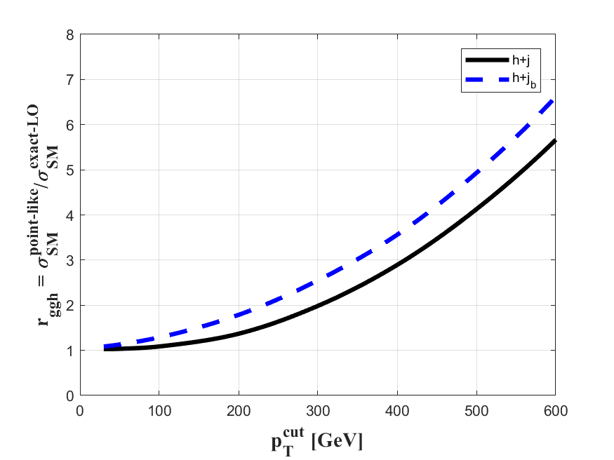
Figure 3: The ratio $r_{ggh}$ defined in Eq. 15, as a function of $p_{T}^{cut}$: $r_{ggh}=\sigma_{SM}^{point-like}(p_{T}^{cut})/\sigma_{SM}^{exact-LO}(p_{T}^{cut})$, where $\sigma_{SM}^{point-like}(p_{T}^{cut})$ and $\sigma_{SM}^{exact-LO}(p_{T}^{cut})$ are the cumulative SM cross-sections which are calculated for a given $p_{T}^{cut}$, using the point-like $ggh$ approximation and the full LO 1-loop set of diagrams, respectively. See also text.

Finally, we wish to briefly address the uncertainty associated with the effective point-like $ggh$ approximation which we use for the calculation of all the SM-like diagrams for $pp\to h+j(j_{b})$ that involve the $ggh$ interaction (i.e., all diagrams in Fig. 2 in the $pp\to h+j$ case and diagram (e) in Fig. 2 for the $pp\to h+j_{b}$ case). As mentioned earlier, for the differential $p_{T}(h)$ distribution, $d\sigma/dp_{T}(h)$, this approximation is accurate up to $p_{T}(h)\>\raisebox{-2.15277pt}{$\stackrel{{\scriptstyle\textstyle<}}{{\sim}}$}\>200$ GeV. As a result, the $p_{T}$-dependent cumulative cross-section defined in Eq. 11 accrues an error which depends on the $p_{T}^{cut}$ used. To estimate the corresponding uncertainty in $\sigma_{SM}(p_{T}^{cut})$, we plot in Fig. 3 the ratio:

$$r_{ggh}\equiv\frac{\sigma_{SM}^{point-like}(p_{T}^{cut})}{\sigma_{SM}^{exact-LO}(p_{T}^{cut})}~{},$$ (15)

as a function of $p_{T}^{cut}$ for both $pp\to h+j$ and $pp\to h+j_{b}$, where $\sigma_{SM}^{point-like}(p_{T}^{cut})$ and $\sigma_{SM}^{exact-LO}(p_{T}^{cut})$ are the cumulative cross-sections which are calculated for a given $p_{T}^{cut}$, using the point-like $ggh$ approximation and the full LO 1-loop set of diagrams (i.e., top-quark loops with a finite top-quark mass), respectively. The loop-induced SM cross-sections were calculated using the loopSM model of MadGraph5.

We see that the point-like $ggh$ approximation overestimates the cumulative cross-sections for exclusive Higgs + jet production, in particular at large $p_{T}(h)$, and that the effect is more pronounced in the Higgs + b-jet case. In particular, for $p_{T}^{cut}=100,~{}200,~{}400$ GeV, we find $r_{ggh}\sim 1,~{}1.4,~{}2.9$ for $pp\to h+j$ and $r_{ggh}\sim 1.3,~{}1.8,~{}3.6$ for $pp\to h+j_{b}$. Thus, by using the effective point-like $ggh$ vertex we are overestimating the Higgs + jet cross-sections (which are dominated by the SM diagrams involving the $ggh$ interaction) and, therefore, the corresponding expected number of Higgs + jet events, roughly by a factor of $r_{ggh}$. On the other hand, as will be shown later, the statistical significance of the signals ($N_{SD}$ defined in Eq. 14 above) only mildly depend on the calculation scheme (i.e., on $r_{ggh}$). We will address these issues in a more quantitative manner below.

III Higgs + jet production in the kappa-framework

The kappa-framework is defined by multiplying the SM couplings $g_{i}$ by a scaling factor $\kappa_{i}$, which parameterizes the effects of NP when it has the same Lorentz structure as the corresponding SM interactions kappa_framework ; 1612.00269 . In the case of $pp\to h+j(j_{b})$, the relevant scaling factors apply to the effective (1-loop) Higgs-gluon interaction of Eq. 4 and to the light and/or b-quark Yukawa couplings. In particular, the effective interaction Lagrangian for $pp\to h+j(j_{b})$ in the kappa-framework, takes the form:

$${\cal L}_{eff}^{h+j}=-\sum_{q=u,d,s,c,b}\kappa_{q}\frac{m_{b}}{v}h\bar{q}q+\kappa_{g}C_{g}hG_{\mu\nu}^{a}G^{\mu\nu,a}~{},$$ (16)

where we have scaled the light-quark Yukawa coupling, $y_{q}$, with the SM b-quark Yukawa:

$$\kappa_{q}\equiv\frac{y_{q}}{y_{b}^{SM}}~{},$$ (17)

and $y_{b}^{SM}=\sqrt{2}m_{b}/v$. In particular, $\kappa_{g}=1$, $\kappa_{b}=1$, $\kappa_{c}\sim 0.3$, $\kappa_{s}\sim{\cal O}(10^{-2})$ and $\kappa_{u,d}\sim{\cal O}(10^{-3})$ are the SM strengths for the corresponding couplings. In what follows, we will refer to the SM case by $\kappa_{u,d,c,s}=0$, since the effect of the small SM values for $\kappa_{u,d,c,s}$ in $pp\to h+j$ are negligible.

III.1 The case of Higgs + light-jet production

As mentioned earlier, in the case of $pp\to h+j$, where $j=g,u,d,s,c$ is a non-flavor tagged light-jet originating from a gluon or any quark of the 1st and 2nd generations, the SM tree-level diagrams involving the light-quarks Yukawa couplings are vanishingly small (see Eqs. 1-3). Therefore, the dominant SM contribution to $\sigma(pp\to h+j)$ arises at 1-loop via the sub-processes $gg\to gh$, $gq\to qh$, $g\bar{q}\to\bar{q}h$ and $q\bar{q}\to gh$ (the corresponding diagrams are depicted in Fig. 2, where the loops are represented by an effective $ggh$ vertex). In particular, using the Higgs-gluon effective Lagrangian of Eq. 4, the corresponding total SM cross-section for $pp\to h+j$ can be written as:

$$\sigma_{SM}^{hj}=C_{g}^{2}\left(\sigma^{gg}_{SM}+\sigma^{gq}_{SM}+\sigma^{g\bar{q}}_{SM}+\sigma^{q\bar{q}}_{SM}\right)~{},$$ (18)

where $\sigma^{ij}_{SM}$, for $ij=gg,gq,g\bar{q},q\bar{q}$, can be obtained from the corresponding squared amplitudes given in Eqs. 5-8. For example, $\sigma^{gg}_{SM}$ is part of the SM cross-section coming from $gg\to gh$, which is the dominant sub-process in the SM.

On the other hand, turning on the light-quark $qqh$ Yukawa couplings and allowing for deviations also in the Higgs-gluon $ggh$ interaction, within the kappa-framework of Eq. 16, we obtain the total NP cross-section for $pp\to h+j$:

$$\sigma^{hj}=\kappa_{g}^{2}\sigma_{SM}^{hj}+\kappa_{q}^{2}\sigma_{qqh}^{hj}~{},$$ (19)

where $\sigma_{SM}^{hj}\simeq\sigma^{hj}(\kappa_{g}=1,\kappa_{q}=0)$ is given in Eq. 18 and $\sigma_{qqh}^{hj}=\sigma^{hj}(\kappa_{g}=0,\kappa_{q}=1)$ arises from the the s-channel and t-channel tree-level $gq\to qh$ diagrams, depicted in Fig. 1, where only the (scaled) light-quarks $qqh$ Yukawa couplings contribute. The interference term between the diagrams involving the $ggh$ and $qqh$ couplings is proportional to the light-quark mass and is, therefore, neglected in Eq. 19. In particular, $\sigma^{hj}$ is practically insensitive to the signs of $\kappa_{g}$ and $\kappa_{q}$.

Furthermore, in the $hgg-h\bar{q}q$ kappa-framework of Eq. 16, the ratio of branching ratios in Eq. 10 is given by:

$$\mu_{h\to ff} \equiv \frac{BR(h\to ff)}{BR_{SM}(h\to ff)}$$ (20)

$$= \frac{1}{1+\left(\kappa_{g}^{2}-1\right)BR_{SM}^{gg}+\kappa_{q}^{2}BR_{SM}^{bb}}~{},$$

where $BR_{SM}^{gg,bb}=BR_{SM}(h\to gg,bb)$ and we will assume no NP in the Higgs decay $h\to ff$. In particular, as mentioned above, we assume that the Higgs decays via $h\to\gamma\gamma$ with a SM decay rate.

Collecting the expressions from Eqs. 10, 19 and 20, we obtain the signal strength in the kappa-framework:

$$\mu_{hj}^{f}=\left(\kappa_{g}^{2}+\kappa_{q}^{2}R^{hj}\right)\cdot\mu_{h\to ff}~{},$$ (21)

where

$$R^{hj}\equiv\frac{\sigma_{qqh}^{hj}}{\sigma_{SM}^{hj}}~{},$$ (22)

is the NP contribution scaled with the SM cross-section and calculated using cumulative cross-sections, as defined in Eq. 11, i.e., for a given $p_{T}^{cut}$ in both numerator and denominator: $R^{hj}=R^{hj}(p_{T}^{cut})=\sigma_{qqh}^{hj}(p_{T}^{cut})/\sigma_{SM}^{hj}(p_{T}^{cut})$. The ratio $R^{hj}$ contains all the dependence of $\mu_{hj}^{f}$ on the Higgs $p_{T}$ and, as will be further discussed below, is where all the uncertainties reside, i.e., the higher order corrections (K-factor), the theoretical uncertainty of the PDF due to variations of the renormalization and factorization scales and the acceptance factors.

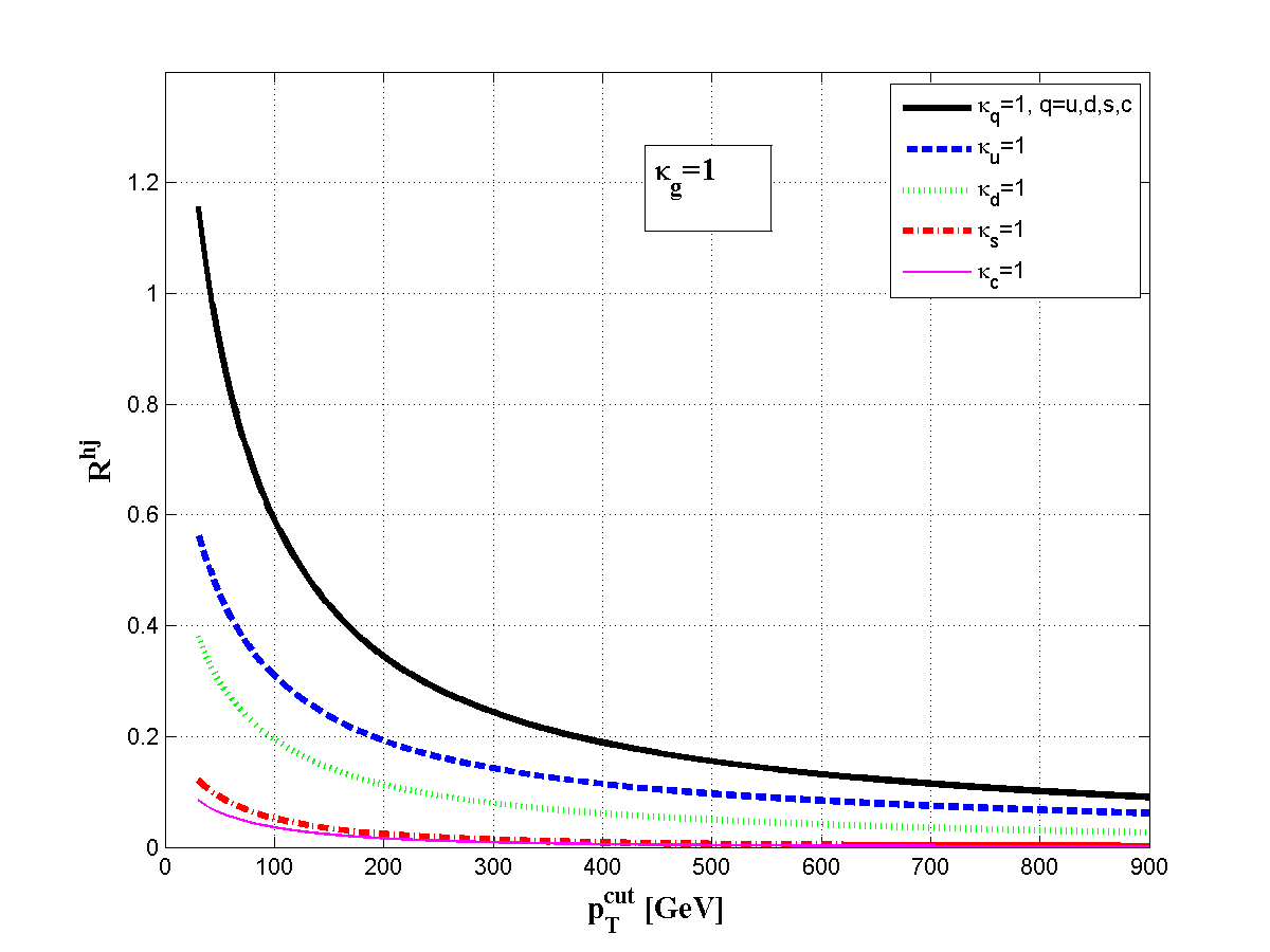
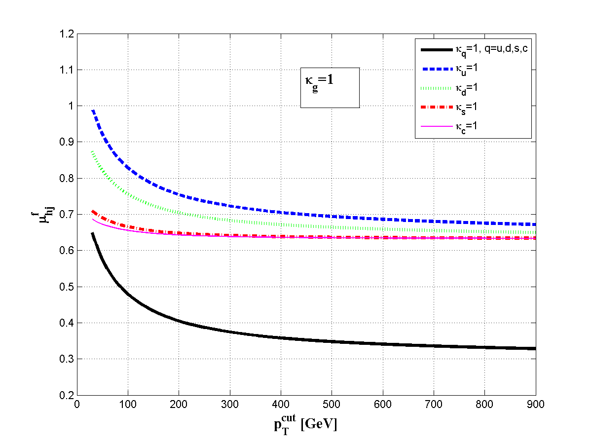
Figure 4: The $p_{T}^{cut}$ dependence of $R^{hj}$ (top) and $\mu_{hj}^{f}$ (bottom), for $\kappa_{g}=1$ (i.e., assuming no NP in the $ggh$ interaction) and the cases $\kappa_{q}=1$ for all $q=u,d,s,c$ (solid line), $\kappa_{u}=1$ (dashed line), $\kappa_{d}=1$ (dotted line), $\kappa_{s}=1$ (dot-dashed line) and $\kappa_{c}=1$ (thin solid line).

In Fig. 4 we show the dependence of $R^{hj}$ and the signal strength, $\mu_{hj}^{f}$, on $p_{T}^{cut}$, assuming no NP in the $hgg$ interaction ($\kappa_{g}=1$) and for the cases in which either a single or all light-quark Yukawa couplings are modified, i.e., $\kappa_{q}=1$ for any one of the light-quarks $q=u,d,s,c$ or $\kappa_{q}=1$ for all $q=u,d,s,c$. We find that the effect of $\kappa_{q}\neq 0$ is to change the softer $p_{T}(h)$ spectrum, so that $R^{hj}$ drops when $p_{T}^{cut}$ is increased. As a result, the contribution of $\kappa_{q}$ to $pp\to h+j$ sharply drops in the harder $p_{T}(h)$ region, $p_{T}(h)\>\raisebox{-2.15277pt}{$\stackrel{{\scriptstyle\textstyle>}}{{\sim}}$}\>300$ GeV, where $R^{hj}\>\raisebox{-2.15277pt}{$\stackrel{{\scriptstyle\textstyle<}}{{\sim}}$}\>{\cal O}(0.1)$, see Fig. 4.

Note, however, that the signal strength approaches an asymptotic value as $p_{T}^{cut}$ is further increased, which corresponds to the region where the $\kappa_{q}$ dependence of $\mu_{hj}^{f}$ is dominated by the decay factor $\mu_{h\to ff}$ in Eq. 20. In particular, $\mu_{hj}^{f}\to 0.6-0.7$ in the single $\kappa_{q}=1$ case and $\mu_{hj}^{f}\to 0.3$ when $\kappa_{q}=1$ for all light-quarks. Thus, in the high Higgs $p_{T}$ regime, the difference between the effects of a single $\kappa_{q}\neq 0$ is small, i.e., for either of the quark flavors $q=u,d,c,s$. The advantage of monitoring the high $p_{T}(h)$ spectrum, where $R^{hj}$ is suppressed is, therefore, reducing the theoretical and experimental uncertainties which, as mentioned above, reside only in $R^{hj}$. Indeed, this will be illustrated in Table 1 below, where we show the sensitivity of the signal to the theoretical uncertainty obtained by scale variations.

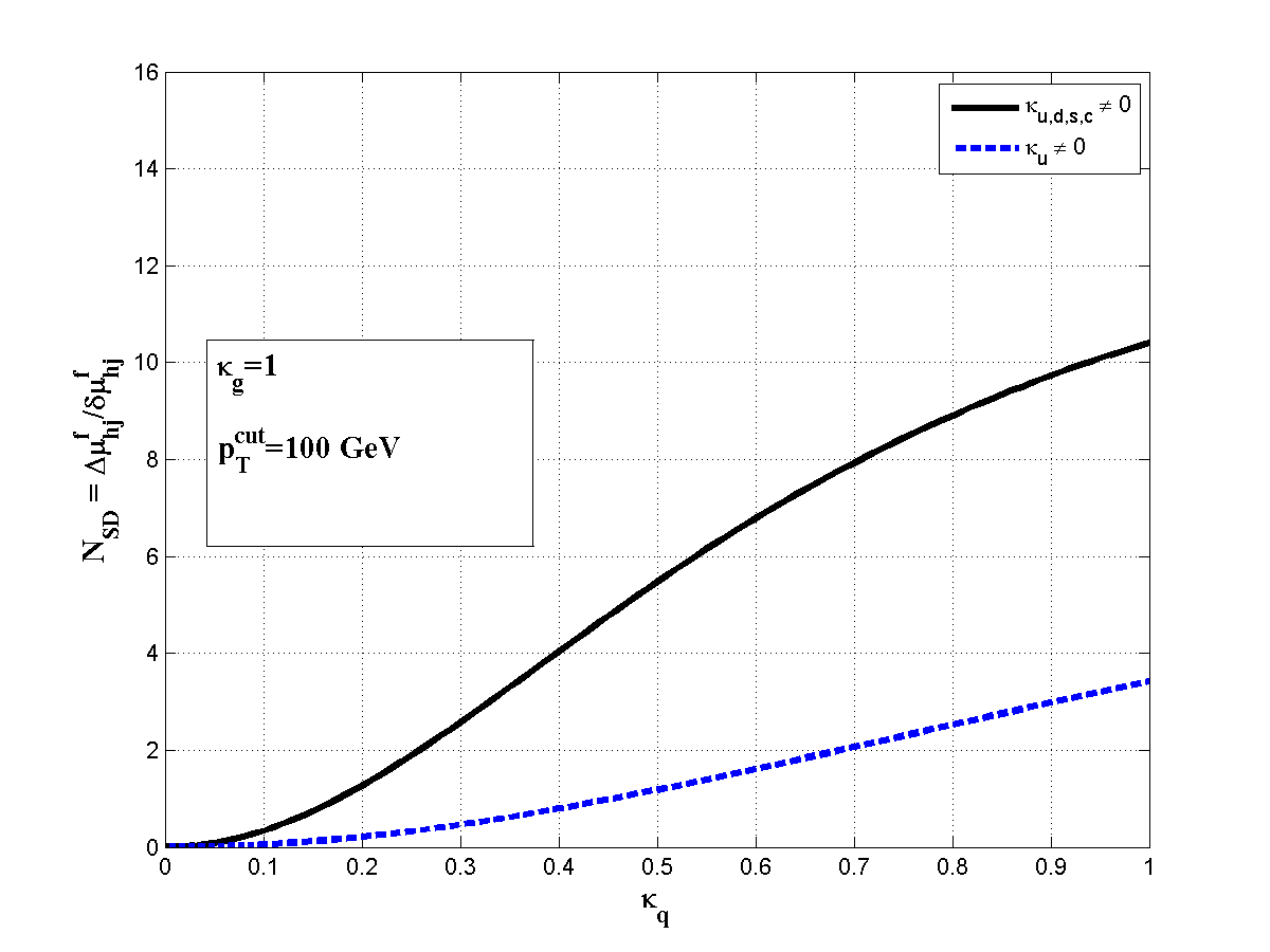
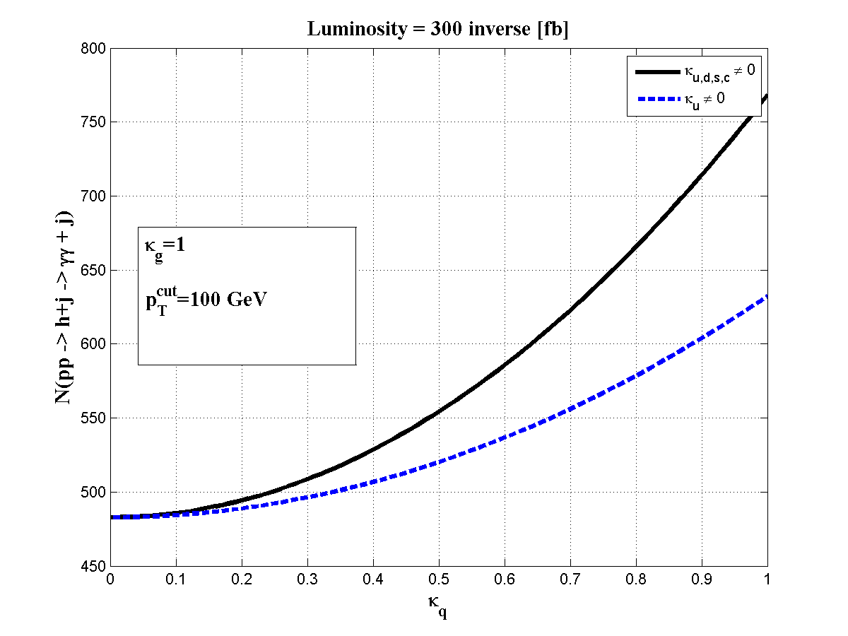
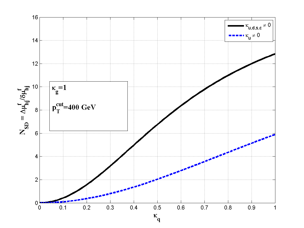
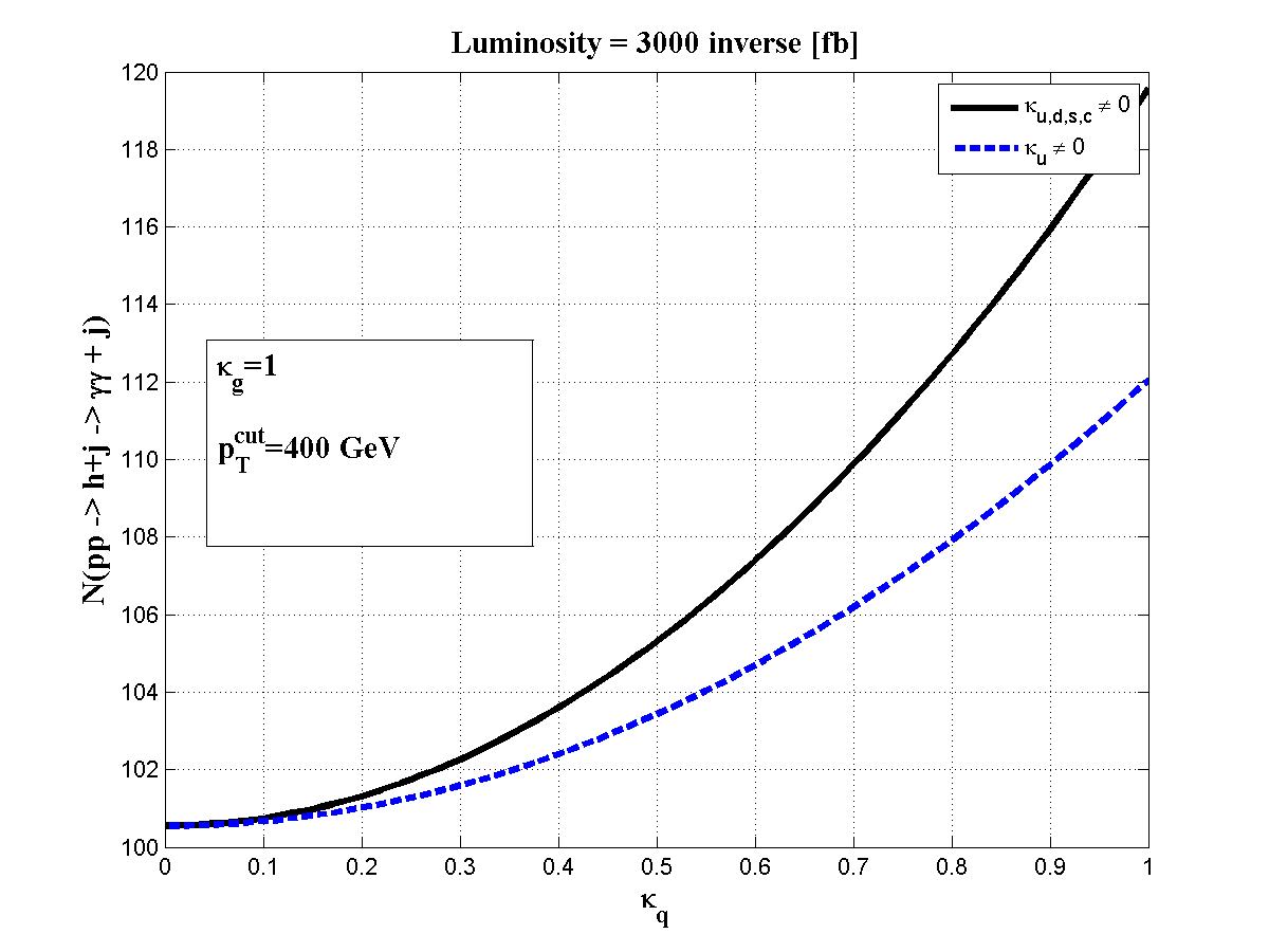
Figure 5: The expected statistical significance, $N_{SD}=\Delta\mu_{hj}^{f}/\delta\mu_{hj}^{f}$, and the number of $pp\to h+j\to\gamma\gamma+j$ events, as a function of $\kappa_{q}$, for $\kappa_{g}=1$ (i.e., assuming no NP in the $hgg$ interaction) and for $p_{T}^{cut}=100$ GeV (upper plots) and $p_{T}^{cut}=400$ GeV (lower plots). The two cases of a single $\kappa_{u}\neq 0$ (dashed line) and $\kappa_{q}\neq 0$ for all $q=u,d,s,c$ (solid line), are considered. We assume a 5% relative error ($\delta\mu_{hj}^{f}=0.05$) and an acceptance of 50% in the event yield, with a luminosity of ${\cal L}=300$ fb^-1 for the $p_{T}^{cut}=100$ GeV case and ${\cal L}=3000$ fb^-1 in the $p_{T}^{cut}=400$ GeV case.

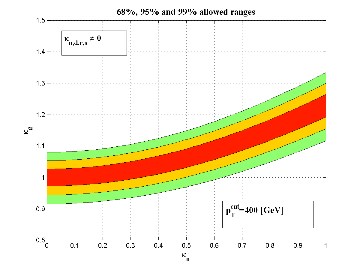
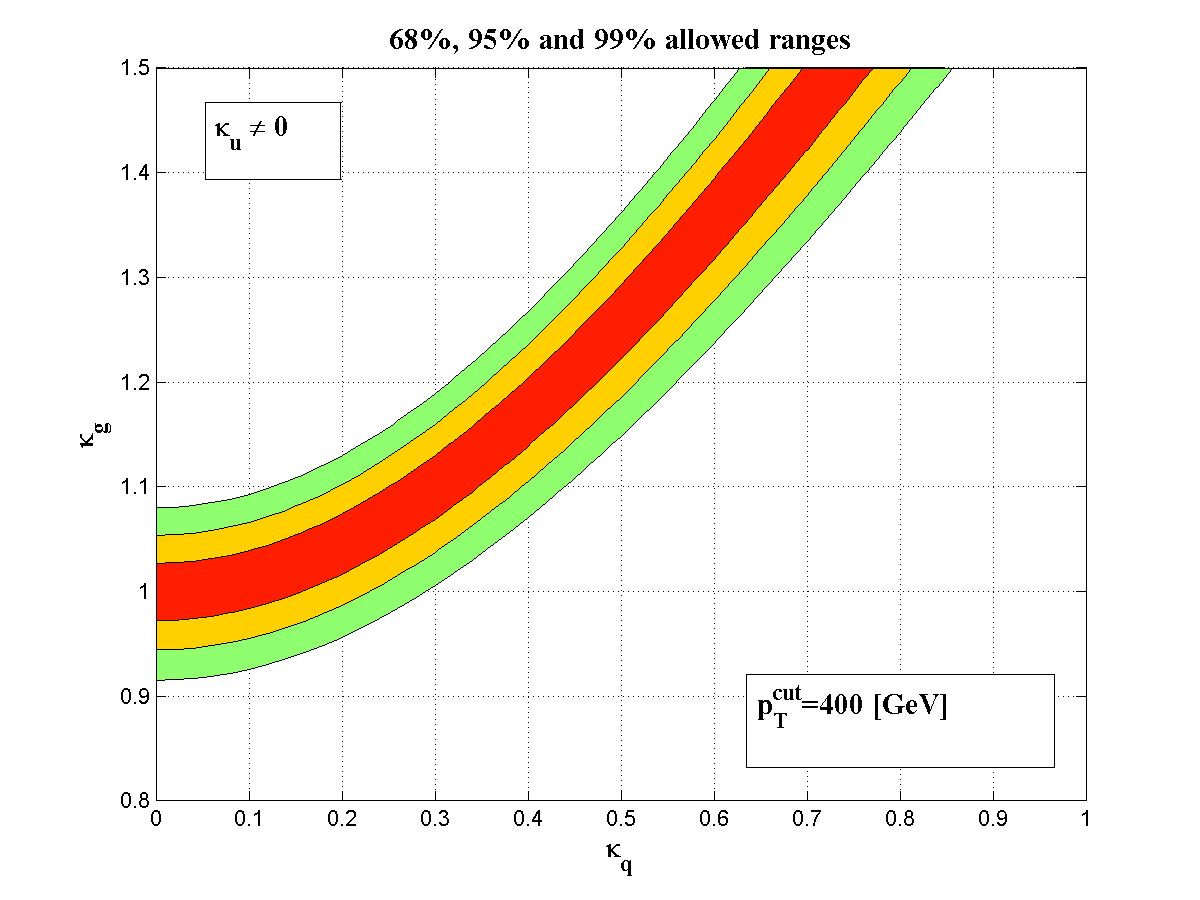
Figure 6: The 68%(red), 95%(orange) and 99%(green) CL sensitivity ranges, corresponding to $\Delta\mu_{hj}^{f}\equiv\left|\mu_{hj}^{f}-1\right|\leq 0.05,~{}0.1$ and $0.15$, respectively, with $p_{T}^{cut}=400$ GeV, in the $\kappa_{u}-\kappa_{g}$ plane for $\kappa_{d}=\kappa_{s}=\kappa_{c}=0$ (top) and in the $\kappa_{q}-\kappa_{g}$ plane for $\kappa_{q}=\kappa_{u}=\kappa_{d}=\kappa_{s}=\kappa_{c}$ (bottom). Recall that $\kappa_{g}=1$ and $\kappa_{u,d,c,s}\to 0$ represent the SM case, see also text.

In Fig. 5 we plot the expected statistical significance, $N_{SD}$ defined in Eq. 14, assuming a 5% relative error ($\delta\mu_{hj}^{f}=0.05$), as a function of $\kappa_{q}$ for two cases: (i) $\kappa_{q}\neq 0$ for all $q=u,d,s,c$ and (ii) only $\kappa_{u}\neq 0$. In both cases we assume no NP in the Higgs-gluon coupling ($\kappa_{g}=1$) and we use two different $p_{T}^{cut}$ values $p_{T}^{cut}=100,~{}400$ GeV. We see that, in the single $\kappa_{u}\neq 0$ case, there is a $3\sigma$ sensitivity to values of $\kappa_{u}\>\raisebox{-2.15277pt}{$\stackrel{{\scriptstyle\textstyle>}}{{\sim}}$}\>0.6$, for $\kappa_{g}=1$ and using $p_{T}^{cut}=400$ GeV. In the case where the NP modifies $\kappa_{q}$ for all $q=u,d,c,s$, one can expect a deviation of more than $3\sigma$ for values of $\kappa_{q}\>\raisebox{-2.15277pt}{$\stackrel{{\scriptstyle\textstyle>}}{{\sim}}$}\>0.3$. We also show in Fig. 5 the corresponding expected number of $pp\to h+j\to\gamma\gamma+j$ events, as a function of $\kappa_{q}$ for cases (i) and (ii) considered above, with $p_{T}^{cut}=100$ and 400 GeV and an integrated luminosity of 300 and 3000 fb^-1, respectively, assuming a signal acceptance of 50%. We can see that around $1000$($100$) $pp\to h+j\to\gamma\gamma+j$ events with $p_{T}(h)>100(400)$ GeV are expected at the LHC(HL-LHC), i.e., with ${\cal L}=300(3000)$ fb^-1. Thus, in both cases it should be possible to probe the NP effects when the Higgs decays via $h\to\gamma\gamma$.

The signal strength $\mu_{hj}^{f}$ is more sensitive to NP in the Higgs-gluon coupling, i.e., to $\kappa_{g}$. We find, for example, that if $\mu_{hj}^{f}$ is known to a $5\%(1\sigma)$ accuracy, then a deviation of more than $3\sigma$ is expected for $\kappa_{g}\>\raisebox{-2.15277pt}{$\stackrel{{\scriptstyle\textstyle<}}{{\sim}}$}\>0.9$ for any value of $\kappa_{q}$ and for any $p_{T}^{cut}\>\raisebox{-2.15277pt}{$\stackrel{{\scriptstyle\textstyle<}}{{\sim}}$}\>500$ GeV. This is illustrated in Fig. 6 where we plot the 68%, 95% and 99% confidence level (CL) allowed ranges in the $\kappa_{q}-\kappa_{g}$ plane, for $p_{T}^{cut}=400$ GeV and assuming that the signal strength has been measured to be $\mu_{hj}^{f}\sim 1\pm 0.05(1\sigma)$, i.e., with a SM central value and to an accuracy of $\delta\mu_{hj}^{f}=5\%(1\sigma)$. Here also, we consider both the single $\kappa_{u}$ case where $\kappa_{u}\neq 0$ and $\kappa_{d}=\kappa_{s}=\kappa_{c}=0$ and the case where $\kappa_{q}\neq 0$ for all $q=u,d,s,c$. In particular, values of $\{\kappa_{q},\kappa_{g}\}$ outside the shaded 99% contour will be excluded at more than $3\sigma$, if the signal strength will be measured to lie within $0.85<\mu_{hj}^{f}<1.15$.

Statistical significance $N_{SD}=\frac{\Delta\mu_{hj}^{f}}{\delta\mu_{hj}^{f}}$
$\kappa_{u}\neq 0$, $\kappa_{d}=\kappa_{s}=\kappa_{c}=0$
	$\kappa_{u}=0$	$\kappa_{u}=0.25$	$\kappa_{u}=0.5$
$\kappa_{g}=0.8$	$6.79$	$7.12^{-0.03}_{+0.03}$	$8.0^{-0.11}_{+0.10}$
$\kappa_{g}=0.9$	$3.53$	$3.97^{-0.03}_{+0.03}$	$5.14^{-0.11}_{+0.10}$
$\kappa_{g}=1.0$	$0$	$0.56^{-0.03}_{+0.03}$	$2.03^{-0.11}_{+0.10}$
$\kappa_{g}=1.1$	$3.78$	$3.09^{+0.03}_{-0.03}$	$1.30^{+0.11}_{-0.10}$
$\kappa_{g}=1.2$	$7.75$	$6.95^{+0.03}_{-0.03}$	$4.84^{+0.11}_{-0.10}$

$\kappa_{q}\neq 0$ for all $q=u,d,s,c$
	$\kappa_{q}=0$	$\kappa_{q}=0.25$	$\kappa_{q}=0.5$
$\kappa_{g}=0.8$	$6.79$	$8.30^{-0.05}_{+0.04}$	$11.13^{-0.13}_{+0.12}$
$\kappa_{g}=0.9$	$3.53$	$5.43^{-0.05}_{+0.04}$	$9.03^{-0.13}_{+0.12}$
$\kappa_{g}=1.0$	$0$	$2.32^{-0.05}_{+0.04}$	$6.74^{-0.13}_{+0.12}$
$\kappa_{g}=1.1$	$3.78$	$1.01^{+0.05}_{-0.04}$	$4.26^{-0.13}_{+0.12}$
$\kappa_{g}=1.2$	$7.75$	$4.55^{+0.04}_{-0.04}$	$1.61^{-0.13}_{+0.11}$

Table 1: The statistical significance of the NP signal for $pp\to h+j$, $N_{SD}=\Delta\mu_{hj}^{f}/\delta\mu_{hj}^{f}$, assuming a 5% error ($\delta\mu_{hj}^{f}=0.05(1\sigma)$), for $p_{T}^{cut}=400$ GeV and for values of the scaled couplings $\kappa_{q}=0,0.25,0.5$ and $\kappa_{g}=0.8,0.9,1,1.1,1.2$, in the single $\kappa_{u}$ case assuming $\kappa_{d}=\kappa_{s}=\kappa_{c}=0$ (top table) and in the case where $\kappa_{q}\neq 0$ for all $q=u,d,s,c$ (bottom table). The errors indicate the theoretical dependence on the PDF scale, where the superscript(subscript) corresponds to twice(half) the nominal scale $\mu_{F}=\mu_{R}=\mu_{T}\equiv\sum_{i}\sqrt{m_{i}^{2}+p_{T}^{2}(i)}$, see also text.

In Table 1 we list the statistical significance of the NP signal, $N_{SD}=\Delta\mu_{h_{b}}^{f}/\delta\mu_{h_{b}}^{f}$, as defined in Eq. 14, again assuming 5% error ($\delta\mu_{hj}^{f}=0.05(1\sigma)$), for $p_{T}^{cut}=400$ GeV and some discrete values of the scaled couplings: $\kappa_{q}=0,0.25,0.5$ and $\kappa_{g}=0.8,0.9,1,1.1,1.2$. Here also, results are given in the single $\kappa_{u}$ case and in the case where $\kappa_{q}\neq 0$ for all $q=u,d,s,c$. We include the theoretical uncertainty obtained by scale variations and (although of little use) write $N_{SD}$ up to the 2nd digit to illustrate the small uncertainty due the scale variation. Note that for $\kappa_{q}=0$ there is no dependence on the scale of the PDF since, in this case, it is cancelled in the ratio of cross-sections as defined in the signal strength $\mu_{hj}^{f}$. We see that indeed the effect of the variation of scale with which the PDF is evaluated is negligible due to the smallness of $R^{hj}$ in the harder $p_{T}$ spectrum, in particular for $p_{T}^{cut}=400$ GeV used in the Table 1 (see also discussion above).

All the results presented in this section were obtained using the effective point-like $ggh$ approximation, which as was shown in section II (see Fig. 3), overestimates the contribution of the SM-like diagrams involving the 1-loop $ggh$ vertex when compared to the 1-loop induced (top-mass dependent) terms. In particular, this approximation effects the denominator of the scaled NP ratio $R^{hj}$ in Eq. 22, i.e., the SM cumulative cross-section $\sigma_{SM}^{hj}(p_{T}^{cut})$. To give a feeling for the sensitivity of our results to the underlying calculation setup at the high $p_{T}(h)$ regime, where the point-like $ggh$ approximation shows ${\cal O}(1)$ deviations, we recalculate the statistical significance $N_{SD}$ in Table 1 using the top-mass dependent 1-loop result for $\sigma_{SM}^{hj}(p_{T}^{cut})$ in Eq. 22. In this case, the scaled NP ratio $R^{hj}$ changes to:

$$R^{hj}\to\tilde{R}^{hj}=r_{ggh}R^{hj}~{},$$ (23)

where $r_{ggh}$, which is defined in Eq. 15, is the ratio between the point-like and the LO loop-induced (mass dependent) SM cross-sections. Thus, replacing $R^{hj}\to\tilde{R}^{hj}$ in the expression of Eq. 21 for the signal strength and using the definition for $N_{SD}$ in Eq. 14, we obtained the statistical significance in the exact 1-loop case:

$$\tilde{N}_{SD}=r_{ggh}N_{SD}-\frac{\left(r_{ggh}-1\right)\left(\tilde{\kappa}_{g}^{2}\mu_{h\to ff}-1\right)}{\delta\mu_{hj}^{f}}~{},$$ (24)

where $\mu_{h\to ff}$ is the scaled Higgs decay branching ratio defined in Eq. 20 and $\delta\mu_{hj}^{f}$ is the assumed $1\sigma$ error (see Eq. 14). Note that in Eq. 24 above we have denoted the the modified $ggh$ interaction by $\tilde{\kappa}_{g}$ (rather than $\kappa_{g}$), since caution has to be taken when interpreting the NP associated with the $ggh$ vertex in the exact top-quark 1-loop case. In particular, in the calculation of $\sigma^{hj}=\sigma(pp\to h+j)$ using the effective point-like $ggh$ interaction, $\kappa_{g}$ simply corresponds to the scaling of the effective $ggh$ SM vertex (see Eq. 16) and, therefore, to the ratio $\kappa_{g}=\sqrt{\sigma^{hj}/\sigma_{SM}^{hj}}$ (see Eq. 19 for $\kappa_{q}=0$). On the other hand, in the exact LO (1-loop) calculation, the diagrams in Fig. 2 involving NP in the effective $ggh$ interaction should be added at the amplitude level to the SM 1-loop diagrams (i.e., with the top-quark loops). Thus, in this case, generic NP effects associated with the $ggh$ vertex in $\sigma^{hj}$ can be parameterized as follows 1312.3317_SMEFT ; 1405.7651 :

$$\sigma^{hj}(\kappa_{q}=0)=\left(\kappa_{t}^{2}+A\kappa_{t}\kappa_{g}+B\kappa_{g}^{2}\right)\sigma_{SM}^{hj}\equiv\tilde{\kappa}_{g}^{2}\sigma_{SM}^{hj}~{},$$ (25)

where $\kappa_{t}\equiv y_{t}/y_{t}^{SM}$ is the $tth$ coupling modifier (which parameterizes potential NP in the SM top-quark loop diagrams) and $A,B$ are phase-space coefficients which depend on the lower Higgs $p_{T}$ cut ($p_{T}^{cut}$), see 1312.3317_SMEFT . Thus, when considering NP in $pp\to h+j$ within the exact 1-loop calculation, the $ggh$ coupling modifier $\tilde{\kappa}_{g}$ (defined in Eq. 25), which appears in Eq. 24 and in Table 2 should be interpreted as the overall NP effect in the $ggh$ interaction, where $\tilde{\kappa}_{g}=\kappa_{t}$ corresponds to NP which modifies only the $tth$ Yukawa coupling while $\tilde{\kappa}_{g}=\sqrt{1+A\kappa_{g}+B\kappa_{g}^{2}}$ applies to the case where $\kappa_{t}=1$ and the NP arises from some other underlying heavy physics which is integrated out and generates the $ggh$ effective interaction of Eq. 16. This interpretation of $\tilde{\kappa}_{g}$ applies to all instances below where we discuss our results for the NP effect in $pp\to h+j(j_{b})$ within the exact LO 1-loop case.

In Table 2 we list the statistical significance $\tilde{N}_{SD}$ calculated according to Eq. 24, again taking a 5% error $\delta\mu_{hj}^{f}=0.05(1\sigma)$, $p_{T}^{cut}=400$ GeV and the same values of the scaled couplings as in Table 2, where here only the single $\kappa_{u}\neq 0$ case is considered. We also list in Table 2 the values of $N_{SD}$ of Table 1 (i.e., corresponding to the case where the diagrams involving the $ggh$ interaction are calculated with the point-like $ggh$ interaction). We see that the expected significance of the NP signal in $pp\to h+j$ is mildly sensitive to the calculation scheme. In particular, variations at the level of $0.1\sigma-1\sigma$ are observed in $N_{SD}$ depending on the values of the scaled NP couplings $\kappa_{q}$ and $\kappa_{g}$ (note that $\tilde{N}_{SD}=N_{SD}$ for $\kappa_{u}=0$), so that the point-like $ggh$ approximation is indeed useful for estimating the NP effect in $pp\to h+j$ even for events with $p_{T}(h)>400$ GeV.

$\tilde{N}_{SD}$ $\left(N_{SD}\right)$
$\kappa_{u}\neq 0$, $\kappa_{d}=\kappa_{s}=\kappa_{c}=0$
	$\kappa_{u}=0$	$\kappa_{u}=0.25$	$\kappa_{u}=0.5$
$\tilde{\kappa}_{g}=0.8$	$6.8(6.8)$	$6.8(7.1)$	$7.0(8.0)$
$\tilde{\kappa}_{g}=0.9$	$3.5(3.5)$	$3.7(4.0)$	$4.1(5.1)$
$\tilde{\kappa}_{g}=1.0$	$0(0)$	$0.3(0.6)$	$1.0(2.0)$
$\tilde{\kappa}_{g}=1.1$	$3.8(3.8)$	$3.4(3.1)$	$2.3(1.3)$
$\tilde{\kappa}_{g}=1.2$	$7.8(7.8)$	$7.2(7.0)$	$5.8(4.8)$

Table 2: The statistical significance of the NP signal for $pp\to h+j$, $\tilde{N}_{SD}$, corresponding to the case where the SM cross-section is calculated exactly (mass dependent) at 1-loop (LO) and given in Eq. 24. As in Table 1, results are shown for 5% error ($\delta\mu_{hj}^{f}=0.05(1\sigma)$), $p_{T}^{cut}=400$ GeV and for values of the scaled couplings $\kappa_{u}=0,0.25,0.5$ and $\tilde{\kappa}_{g}=0.8,0.9,1,1.1,1.2$, in the single $\kappa_{u}\neq 0$ case assuming $\kappa_{d}=\kappa_{s}=\kappa_{c}=0$. We also list in parenthesis the corresponding values of the statistical significance $N_{SD}$ for the case where the SM cross-section is calculated with the point-like $ggh$ approximation. See also text.

III.2 The case of Higgs + b-jet production

We next turn to Higgs + b-jet production, which can be described in the five flavor scheme (5FS), where one treats the b-quark as a massless parton while keeping its Yukawa coupling finite 5FS_hbjet , see also 1010.2977_hbjet4LO ; 1007.5411_hbjet3_NLO . In particular, the LO contribution to $pp\to h+j_{b}$ arises at tree-level by the same diagrams that drive the subprocess $qg\to hq$ (and the charged conjugate one $g\bar{b}\to\bar{b}h$), shown in Fig. 1 with $q=b$. The cross-section for these diagrams is proportional to the $bbh$ Yukawa coupling (squared) and can be obtained from the corresponding squared amplitudes which are given in Eqs. 1-3. The 1-loop contribution to $gb\to bh$, which, in the infinite top-quark mass limit, can be described by the effective $ggh$ vertex (see Fig. 2), is given in Eqs. 6-8. It is comparable to the LO tree-level one at low $p_{T}(h)\>\raisebox{-2.15277pt}{$\stackrel{{\scriptstyle\textstyle<}}{{\sim}}$}\>100$ GeV, while it dominates at the higher $p_{T}(h)$ spectrum (see below).^[2]

Let us denote the corresponding tree-level and 1-loop cumulative cross-sections (following Eq. 11) for $pp\to h+j_{b}$ as $\sigma_{bbh}^{hj_{b}}\equiv\sigma_{bbh}^{hj_{b}}(p_{T}^{cut})$ and $\sigma_{ggh}^{hj_{b}}\equiv\sigma_{ggh}^{hj_{b}}(p_{T}^{cut})$, respectively. Thus, in the kappa-framework where $\kappa_{b}$ and $\kappa_{g}$ are the only NP scaled couplings, the total Higgs + b-jet cross-section is (again there is negligible interference between the diagrams involving the $bbh$ and $ggh$ interactions):

$$\sigma^{hj_{b}}=\kappa_{g}^{2}\sigma_{ggh}^{hj_{b}}+\kappa_{b}^{2}\sigma_{bbh}^{hj_{b}}~{},$$ (26)

so that the SM cross-section is obtained for $\kappa_{g}=\kappa_{b}=1$, i.e., $\sigma_{SM}^{hj_{b}}=\sigma_{ggh}^{hj_{b}}+\sigma_{bbh}^{hj_{b}}$.

The signal strength for $pp\to h+j_{b}\to ff+j_{b}$ is then given by:

$$\mu_{hj_{b}}^{f} = \frac{{\cal N}(pp\to h+j_{b}\to ff+j_{b})}{{\cal N}_{SM}(pp\to h+j_{b}\to ff+j_{b})}$$ (27)

$$\simeq \left(\frac{\kappa_{g}^{2}}{1+R^{hj_{b}}}+\frac{\kappa_{b}^{2}}{1+\left(R^{hj_{b}}\right)^{-1}}\right)\cdot\mu_{h\to ff}^{b}~{},$$

where

$$R^{hj_{b}}\equiv\frac{\sigma_{bbh}^{hj_{b}}}{\sigma_{ggh}^{hj_{b}}}~{},$$ (28)

and

$$\mu_{h\to ff}^{b} \equiv \frac{BR(h\to ff)}{BR_{SM}(h\to ff)}$$ (29)

$$= \frac{1}{1+\left(\kappa_{g}^{2}-1\right)BR_{SM}^{gg}+\left(\kappa_{b}^{2}-1\right)BR_{SM}^{bb}}~{}.$$

Once again, all the uncertainties associated with the measurement of $\mu_{hj_{b}}^{f}$ reside in the ratio of cross-sections $R^{hj_{b}}$ and in the limit $R^{hj_{b}}\ll 1$, we get an expression for $\mu_{hj_{b}}^{f}$ which is similar to the one obtained for the Higgs + light-jet case in Eq. 21, with the replacement $\kappa_{q}\to\kappa_{b}$:

$$\mu_{hj_{b}}^{f}(R^{hj_{b}}\ll 1)\simeq\left(\kappa_{g}^{2}+\kappa_{b}^{2}R^{hj_{b}}\right)\cdot\mu_{h\to ff}^{b}~{}.$$ (30)

In particular, we find that, as in the Higgs + light-jet case, the $\kappa_{b}$ term is important for softer $p_{T}(h)$ for which $R^{hj_{b}}\sim{\cal O}(1)$, while the $\kappa_{g}$ contribution is dominant at the harder $p_{T}(h)$ regime, where $R^{hj_{b}}\ll 1$. For example, we obtain $R^{hj_{b}}\sim 2$ for $p_{T}^{cut}\sim 35$ GeV, dropping to $R^{hj_{b}}\sim 1$ at $p_{T}^{cut}\sim 90$ GeV (i.e., the point where $\sigma_{bbh}^{hj_{b}}$ is comparable to $\sigma_{ggh}^{hj_{b}}$), then to $R^{hj_{b}}\sim 0.4$ for $p_{T}^{cut}\sim 200$ GeV and further to $R^{hj_{b}}\sim 0.15$ at $p_{T}^{cut}\sim 400$ GeV. Thus, here also, the effects of higher-order corrections and variation of scales, as well as the acceptance factors, become insignificant when the signal strength is evaluated for a high $p_{T}^{cut}\sim 400$ GeV, for which $R^{hj_{b}}\sim{\cal O}(0.1)$.

In Fig. 7 we show the dependence of the signal strength $\mu_{hj_{b}}^{f}$ on $p_{T}^{cut}$, assuming no NP in the Higgs-gluon $ggh$ interaction ($\kappa_{g}=1$) and for values of $\kappa_{b}$ within $0<\kappa_{b}<1.5$, which are consistent with the current measurements of the 125 GeV Higgs production and decay processes 1606.02266 . We see that, once again, the signal strength approaches an asymptotic value (for a given $\kappa_{b}$ value) as $p_{T}^{cut}$ is increased, which is where the $\kappa_{g}$ term dominates and the $\kappa_{b}$ dependence arises mostly from the decay factor $\mu_{h\to ff}^{b}$ in Eq. 29.

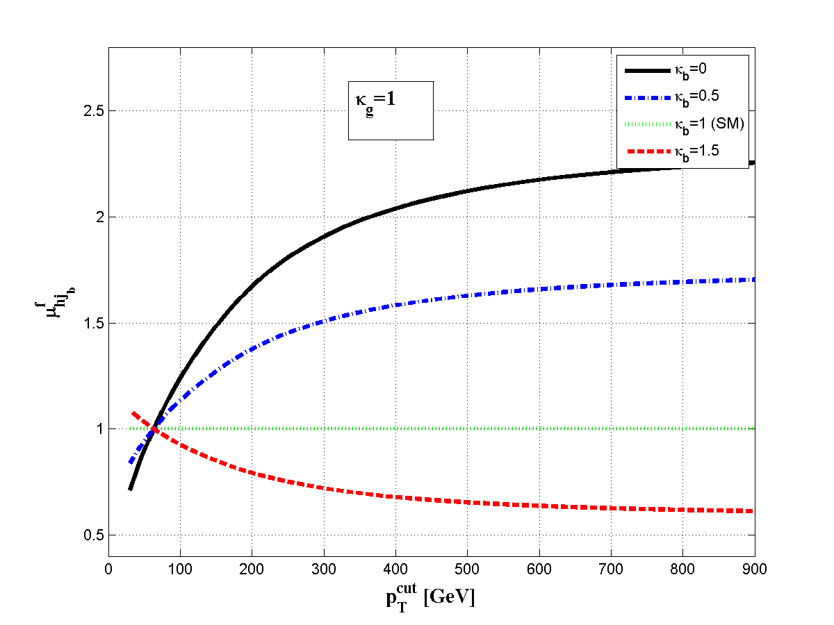
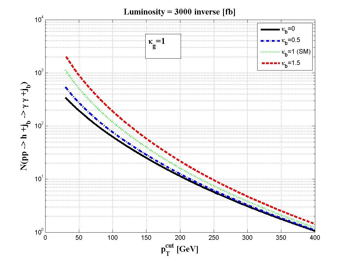
Figure 7: The $p_{T}^{cut}$ dependence of $\mu_{hj_{b}}^{f}$ (top) and of the expected number of events $N(pp\to h+j_{b}\to\gamma\gamma+j_{b})={\cal L}\cdot\sigma(pp\to h+j_{b})\cdot BR(h\to\gamma\gamma)\cdot{\cal A}\cdot\epsilon_{b}$ (bottom) at the HL-LHC with ${\cal L}=3000~{}{\rm fb}^{-1}$, an acceptance of ${\cal A}=0.5$ and a b-jet tagging efficiency of $\epsilon_{b}=0.7$. The curves are for $\kappa_{g}=1$ (i.e., assuming no NP in the $ggh$ interaction) and for $\kappa_{b}=0,0.5,1,1.5$ ($\kappa_{b}=1$ corresponds to the SM case where $\mu_{hj_{b}}^{f}=1$).

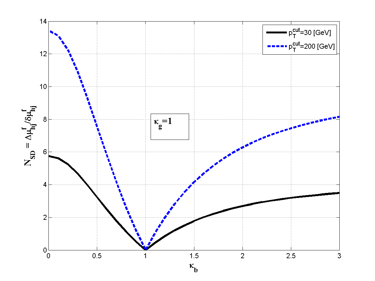
Figure 8: The statistical significance, $N_{SD}=\Delta\mu_{hj_{b}}^{f}/\delta\mu_{hj_{b}}^{f}$, as a function of $\kappa_{b}$ for $p_{T}^{cut}=30$ GeV (solid line) and $p_{T}^{cut}=200$ GeV (dashed line), assuming $\kappa_{g}=1$ and a $5\%(1\sigma)$ error $\delta\mu_{hj_{b}}^{f}=0.05$. See also text.

We also show in Fig. 7 the expected number of $pp\to h+j_{b}\to\gamma\gamma+j_{b}$ events, $N(pp\to h+j_{b}\to\gamma\gamma+j_{b})={\cal L}\cdot\sigma(pp\to h+j_{b})\cdot BR(h\to\gamma\gamma)\cdot{\cal A}\cdot\epsilon_{b}$, as a function of $p_{T}^{cut}$ at the HL-LHC with ${\cal L}=3000$ fb^-1, an acceptance of ${\cal A}=0.5$ and a b-jet tagging efficiency of 70%, i.e., $\epsilon_{b}=0.7$. We see that, under these conditions and for the values of $\kappa_{g}$ and $\kappa_{b}$ considered, a $p_{T}^{cut}\>\raisebox{-2.15277pt}{$\stackrel{{\scriptstyle\textstyle<}}{{\sim}}$}\>100$ GeV is required to ensure ${\cal O}(100)$ $pp\to h+j_{b}\to\gamma\gamma+j_{b}$ events. In particular, ${\cal N}(pp\to h+j_{b}\to\gamma\gamma+j_{b})\sim{\cal O}(1000)$ for $p_{T}^{cut}\sim 30$ GeV and ${\cal N}(pp\to h+j_{b}\to\gamma\gamma+j_{b})\sim{\cal O}(10)$ for $p_{T}^{cut}\sim 200$ GeV, respectively.

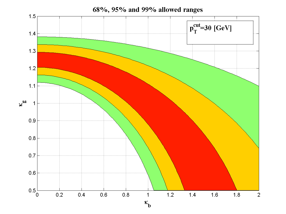
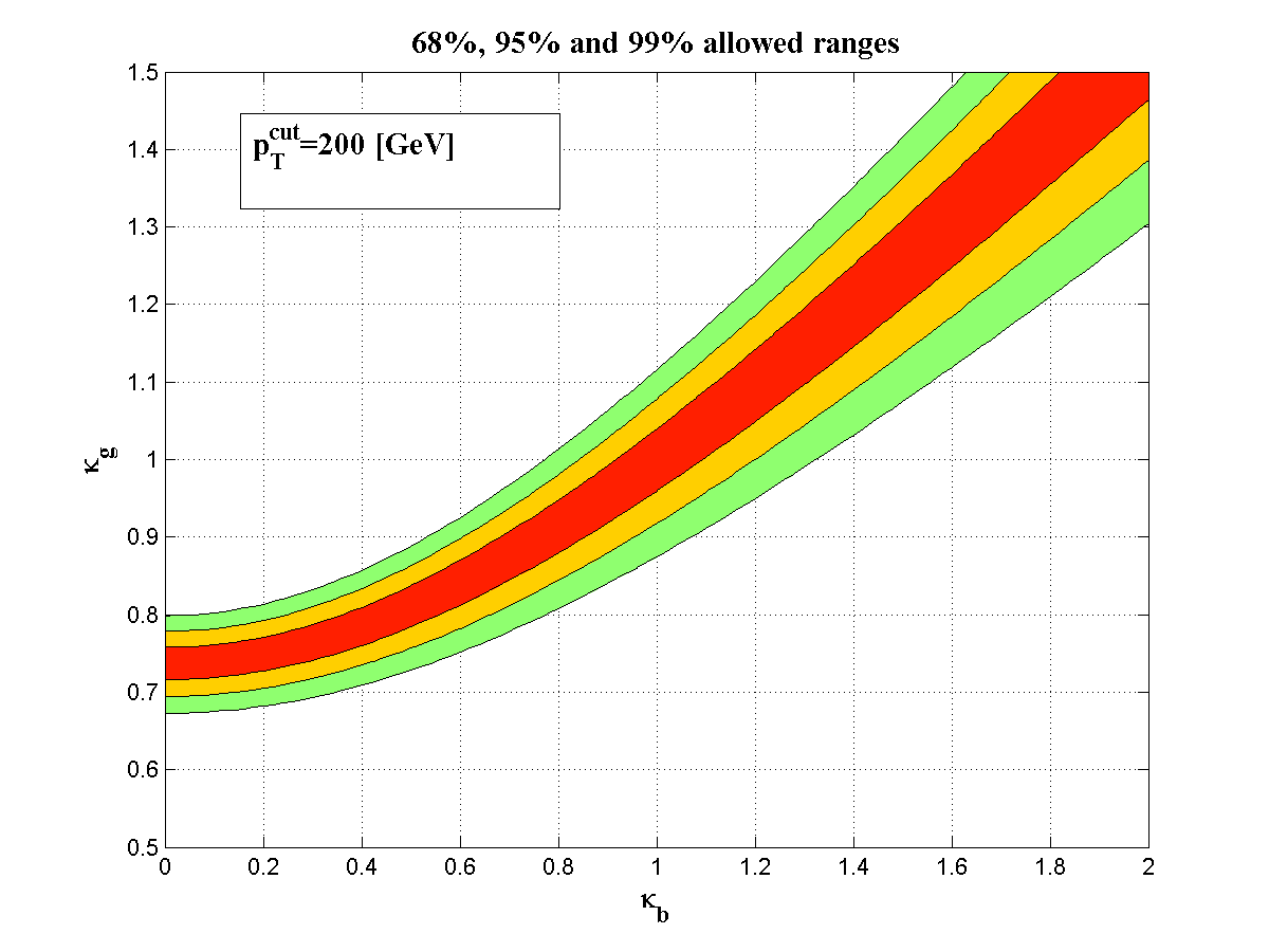
Figure 9: The 68%(red), 95%(orange) and 99%(green) CL allowed ranges in the $\kappa_{b}-\kappa_{g}$ plane, corresponding to $\Delta\mu_{hj}^{f}\equiv\left|\mu_{hj}^{f}-1\right|\leq 0.05,~{}0.1$ and $0.15$, respectively, for $pp\to h+j_{b}$ events with $p_{T}(h)>30$ GeV (top) and $p_{T}(h)>200$ GeV (bottom).

Statistical significance $N_{SD}=\frac{\Delta\mu_{hj_{b}}^{f}}{\delta\mu_{hj_{b}}^{f}}$
	$\kappa_{b}=0.5$	$\kappa_{b}=0.75$	$\kappa_{b}=1$	$\kappa_{b}=1.25$	$\kappa_{b}=1.5$
$\kappa_{g}=0.8$	$0.4^{+0.6}_{-0.3}$	$2.8^{+0.08}_{-0.08}$	$4.6^{-0.3}_{+0.3}$	$6.0^{-0.6}_{+0.6}$	$6.9^{-0.7}_{+0.7}$
$\kappa_{g}=0.9$	$3.5^{-0.8}_{+0.8}$	$0.2^{-0.08}_{+0.3}$	$2.4^{-0.2}_{+0.2}$	$4.3^{-0.4}_{+0.4}$	$5.6^{-0.7}_{+0.7}$
$\kappa_{g}=1.0$	$7.5^{-1.0}_{+1.0}$	$3.3^{-0.4}_{+0.5}$	$0$	$2.4^{-0.3}_{+0.3}$	$4.2^{-0.6}_{+0.6}$
$\kappa_{g}=1.1$	$11.8^{-1.3}_{+1.3}$	$6.7^{-0.7}_{+0.7}$	$2.6^{-0.2}_{+0.2}$	$0.4^{-0.2}_{+0.2}$	$2.6^{-0.5}_{+0.5}$
$\kappa_{g}=1.2$	$16.1^{-1.5}_{+1.5}$	$10.2^{-0.9}_{+0.9}$	$5.3^{-0.3}_{+0.3}$	$1.7^{-0.07}_{+0.07}$	$0.9^{-0.4}_{+0.4}$

Table 3: The statistical significance of the NP signal for $pp\to h+j_{b}$, $N_{SD}=\Delta\mu_{hj_{b}}^{f}/\delta\mu_{hj_{b}}^{f}$, assuming $\delta\mu_{hj_{b}}^{f}=0.05(1\sigma)$, for $p_{T}^{cut}=200$ GeV and for values of the scaled couplings $\kappa_{b}=0.5,0.75,1,1.25,1.5$ and $\kappa_{g}=0.8,0.9,1,1.1,1.2$. The errors indicate the theoretical uncertainty obtained by scale variations, where the superscript(subscript) corresponds to twice(half) the nominal scale $\mu_{F}=\mu_{R}=\mu_{T}\equiv\sum_{i}\sqrt{m_{i}^{2}+p_{T}^{2}(i)}$, see also text.

In the following, we will therefore use $p_{T}^{cut}=30$ GeV and 200 GeV as two representative extreme cases, where the former can be detected in the $pp\to h+j_{b}\to\gamma\gamma+j_{b}$ channel, while the latter is more suited for a higher statistics channel, such as $pp\to h+j_{b}\to WW^{\star}+j_{b}$ followed by the leptonic W-decays $WW^{\star}\to 2\ell 2\nu$, which has a rate about five times larger than $pp\to h+j_{b}\to\gamma\gamma+j_{b}$. In Fig. 8 we plot the statistical significance of the signals, $N_{SD}=\Delta\mu_{hj_{b}}^{f}/\delta\mu_{hj_{b}}^{f}$, for $p_{T}^{cut}=30$ and 200 GeV, as a function of $\kappa_{b}$, assuming $\kappa_{g}=1$ and a $5\%(1\sigma)$ error $\delta\mu_{hj_{b}}^{f}=0.05$. We see that, for $p_{T}^{cut}=200$ GeV a $3\sigma$ effect is expected if $\kappa_{b}\>\raisebox{-2.15277pt}{$\stackrel{{\scriptstyle\textstyle<}}{{\sim}}$}\>0.8$ and/or $\kappa_{b}\>\raisebox{-2.15277pt}{$\stackrel{{\scriptstyle\textstyle>}}{{\sim}}$}\>1.3$, while for $p_{T}^{cut}=30$ GeV a larger deviation from the SM is required, i.e., $\kappa_{b}\>\raisebox{-2.15277pt}{$\stackrel{{\scriptstyle\textstyle<}}{{\sim}}$}\>0.5$ and/or $\kappa_{b}\>\raisebox{-2.15277pt}{$\stackrel{{\scriptstyle\textstyle>}}{{\sim}}$}\>2.2$, for a statistically significant signal of NP in $pp\to h+j_{b}\to\gamma\gamma+j_{b}$.

In Fig. 9 we plot the 68%, 95% and 99% CL sensitivity ranges of NP in the $\kappa_{b}-\kappa_{g}$ plane, for $pp\to h+j_{b}$ with $p_{T}^{cut}=30$ GeV and $p_{T}^{cut}=200$ GeV, assuming again that $\mu_{hj}^{f}\sim 1\pm 0.05(1\sigma)$, i.e., around the SM value with a $5\%(1\sigma)$ accuracy. We see that the two $p_{T}^{cut}$ cases probe different regimes in the $\kappa_{g}-\kappa_{b}$ plane and are, therefore, complementary.

Finally, in Table 3 we list the statistical significance of NP in $pp\to h+j_{b}$, for $\delta\mu_{hj_{b}}^{f}=0.05(1\sigma)$, $p_{T}^{cut}=200$ GeV and for several discrete values of the scaled couplings: $\kappa_{b}=0.5,0.75,1,1.25,1.5$ and $\kappa_{g}=0.8,0.9,1,1.1,1.2$. We include again the theoretical uncertainty obtained by scale variations, which we find to be somewhat higher than in the case of $pp\to h+j$.

Here also we can estimate the sensitivity of the signal to the calculational setup, using the prescription described in the previous section. In particular, we find that calculating $R^{hj_{b}}$ in Eq. 28 with the exact 1-loop finite top-quark mass effect in $\sigma_{ggh}^{hj_{b}}$, the statistical significance values quoted in Table 3 can vary by up to a few standard deviations depending on the values of the scaled couplings $\tilde{\kappa}_{g}$ and $\kappa_{b}$. For example, for $(\kappa_{b},\tilde{\kappa}_{g})=(0.5,0.8),(0.5,1.0),(0.75,1.1),(1.0,1.2),(1.25,0.8)$ (see the definition of $\tilde{\kappa}_{g}$ in Eq. 25 and discussion therein), the expected statistical significance changes from $N_{SD}=0.4,7.5,6.7,5.3,6.0$ in the point-like $ggh$ approximation to $\tilde{N}_{SD}=2.3,4.0,4.4,4.1,4.0$ in the loop-induced (top-quark mass dependent) case.

IV Higgs + jet production in the SMEFT

The SMEFT is defined by expanding the SM Lagrangian with an infinite series of higher dimensional operators, ${\cal O}_{i}^{(n)}$ (using only the SM fields), as EFTpapers ; warsha :

$${\cal L}_{SMEFT}={\cal L}_{SM}+\sum_{n=5}^{\infty}\frac{1}{\Lambda^{(n-4)}}{\sum_{i}f_{i}^{(n)}{\cal O}_{i}^{(n)}}~{},$$ (31)

where $\Lambda$ is the scale of the NP that underlies the SM, $n$ denotes the dimension and $i$ all other distinguishing labels.

Considering the expansion up to operators of dimension 6 (for a complete list of dimension 6 operators in the SMEFT, see e.g. warsha ), we will study here the following subset of operators that can potentially modify the Higgs + jet production processes:

$${\cal O}_{u\phi} = \left(\phi^{\dagger}\phi\right)\left(\bar{Q}_{L}\tilde{\phi}u_{R}\right)+h.c.~{},$$ (32)

$${\cal O}_{d\phi} = \left(\phi^{\dagger}\phi\right)\left(\bar{Q}_{L}\phi d_{R}\right)+h.c.~{},$$ (33)

$${\cal O}_{ug} = \left(\bar{Q}_{L}\sigma^{\mu\nu}T^{a}u_{R}\right)\tilde{\phi}G_{\mu\nu}^{a}+h.c.~{},$$ (34)

$${\cal O}_{dg} = \left(\bar{Q}_{L}\sigma^{\mu\nu}T^{a}d_{R}\right)\phi G_{\mu\nu}^{a}+h.c.~{},$$ (35)

$${\cal O}_{\phi g} = \left(\phi^{\dagger}\phi\right)G_{\mu\nu}^{a}G^{a,\mu\nu}~{},$$ (36)

where $\phi$ is the SM Higgs doublet (with $\tilde{\phi}\equiv i\sigma_{2}\phi^{\star}$), $G^{a,\mu\nu}$ denotes the QCD gauge-field strength and $Q_{L}$ and $u_{R}(d_{R})$ are the ${\rm SU(2)}_{L}$ quark doublet and charge 2/3(-1/3) singlets, respectively.

In particular, we assume that the physics which underlies Higgs+jet production is contained within (dropping the dimension index $n=6$):

$${\cal L}_{SMEFT}={\cal L}_{SM}+\sum_{i=u\phi,d\phi,ug,dg,\phi g}\frac{f_{i}}{\Lambda_{i}^{2}}{\cal O}_{i}~{},$$ (37)

and, to be as general as possible, we allow different scales of the NP which underly the different operators. For example, $\Lambda_{u\phi}$ corresponds to the typical scale of ${\cal O}_{u\phi}$, where by “typical scale” we mean that the corresponding Wilson coefficient is $f_{u\phi}\sim{\cal O}(1)$.

The effects of the operators ${\cal O}_{u\phi},~{}{\cal O}_{d\phi}$ and ${\cal O}_{\phi g}$ can be “mapped” into the kappa-framework, satisfying:

$$\kappa_{q}\simeq\frac{y_{q}^{SM}}{y_{b}^{SM}}-\frac{f_{q\phi}}{y_{b}^{SM}}\frac{v^{2}}{\Lambda_{q\phi}^{2}}~{}~{},~{}~{}\kappa_{g}=1+\frac{12\pi f_{\phi g}}{\alpha_{s}}\frac{v^{2}}{\Lambda_{\phi g}^{2}}~{},$$ (38)

where $y_{q}^{SM}/y_{b}^{SM}\to 0$ for e.g., $q=u~{}{\rm or}~{}d$, while $y_{q}^{SM}/y_{b}^{SM}=1$ for the b-quark. Thus, the sensitivity of the signal strength $\mu_{hj}^{f}$ for $pp\to h+j$ (defined in Eqs. 9 and 10) to the effective Lagrangian containing the operators ${\cal O}_{u\phi},~{}{\cal O}_{d\phi}$ and ${\cal O}_{\phi g}$ can be obtained from the analysis that has been performed for the kappa-framework in the previous section. For example, it follows from Eq. 38 that, for $f_{u\phi},~{}f_{\phi g}\sim{\cal O}(1)$, one expects $|\kappa_{u}|\>\raisebox{-2.15277pt}{$\stackrel{{\scriptstyle\textstyle<}}{{\sim}}$}\>0.5$ and $\Delta\kappa_{g}=|\kappa_{g}-1|\>\raisebox{-2.15277pt}{$\stackrel{{\scriptstyle\textstyle>}}{{\sim}}$}\>0.1$, if the corresponding scales of NP are $\Lambda_{u\phi}\>\raisebox{-2.15277pt}{$\stackrel{{\scriptstyle\textstyle>}}{{\sim}}$}\>3$ TeV and $\Lambda_{\phi g}\>\raisebox{-2.15277pt}{$\stackrel{{\scriptstyle\textstyle<}}{{\sim}}$}\>15$ TeV, respectively.

On the other hand, the (flavor diagonal) operators ${\cal O}_{ug}$ and ${\cal O}_{dg}$ induce new chromo-magnetic dipole moment (CMDM) type, $qqg$ and contact $qqgh$ interactions, which have a new Lorentz structure and, therefore, cannot be described by scaling the SM couplings. In particular, these new CMDM-like operators give rise to different Higgs + jet kinematics with respect to the SM. The effects of the light-quarks and b-quark CMDM-like effective operators, ${\cal O}_{qg}$ ($q=u,d,c,s,b$), in Higgs production at the LHC was studied in 1411.0035 ; hbjet2_bMM , where it was found that the inclusive Higgs production, $pp\to h+X$, and Higgs + b-jets events can be used to probe the CMDM-like interactions if its typical scale is $\Lambda_{qg}\sim{\rm few}$ TeV. Here we will show that a better sensitivity to the scale of the effective quark CMDM-like operators, $\Lambda_{qg}$, can be achieved by analysing the exclusive $pp\to h+j(j_{b})\to\gamma\gamma+j(j_{b})$ Higgs production and decay channels and using the signal strength formalism with the cumulative cross-sections for a high $p_{T}^{cut}\sim 200-300$ GeV.

Note that, in the general case where the Wilson coefficients $f_{u\phi}$, $f_{d\phi}$, $f_{ug}$ and $f_{dg}$ are arbitrary $3\times 3$ matrices in flavor space, the operators ${\cal O}_{u\phi}$, ${\cal O}_{d\phi}$, ${\cal O}_{ug}$ and ${\cal O}_{dg}$ will generate tree-level flavor-violating $u_{i}\to u_{j}$ and $d_{i}\to d_{j}$ transitions ($i,j=1-3$ are flavor indices). One way to avoid that is to assume proportionality of these Wilson coefficients to the corresponding $3\times 3$ Yukawa coupling matrices ($Y_{u}$ and $Y_{d}$), in which case the field redefinitions which diagonalize the quark matrices also diagonalize these operators and the effective theory is automatically minimally-flavor-violating (MFV). That is,

$$\frac{f}{\Lambda^{2}}{\cal O}_{ug}\to Y_{q}\cdot\frac{f_{MFV}}{\Lambda^{2}_{MFV}}{\cal O}_{ug}~{},$$ (39)

so that the relation between generic NP parameters $(f,\Lambda)$ and the corresponding parameters in the MFV effective theory is (for a single flavor $q$):

$$\frac{\Lambda_{MFV}^{2}}{\Lambda^{2}}=y_{q}\frac{f_{MFV}}{f}~{}.$$ (40)

Thus, if $f_{MFV}\sim f$, then $\Lambda_{MFV}\sim\sqrt{y_{q}}\cdot\Lambda$, in which case $\Lambda_{MFV}\ll\Lambda$ for $q\neq t$. On the other hand, for $\sqrt{y_{q}f_{MFV}/f}\sim{\cal O}(1)$ we have $\Lambda_{MFV}\sim\Lambda$. In what follows we would like to keep our discussion as general as possible, not restricting to any assumption about the possible flavor structure of the Wilson coefficients. In particular, we will focus below on a single flavor (diagonal element) of these operators and assume that flavor violation is controlled by some underlying mechanism in the high-energy theory (not necessarily MFV), thereby suppressing the non-diagonal elements of these operators to an acceptable level.

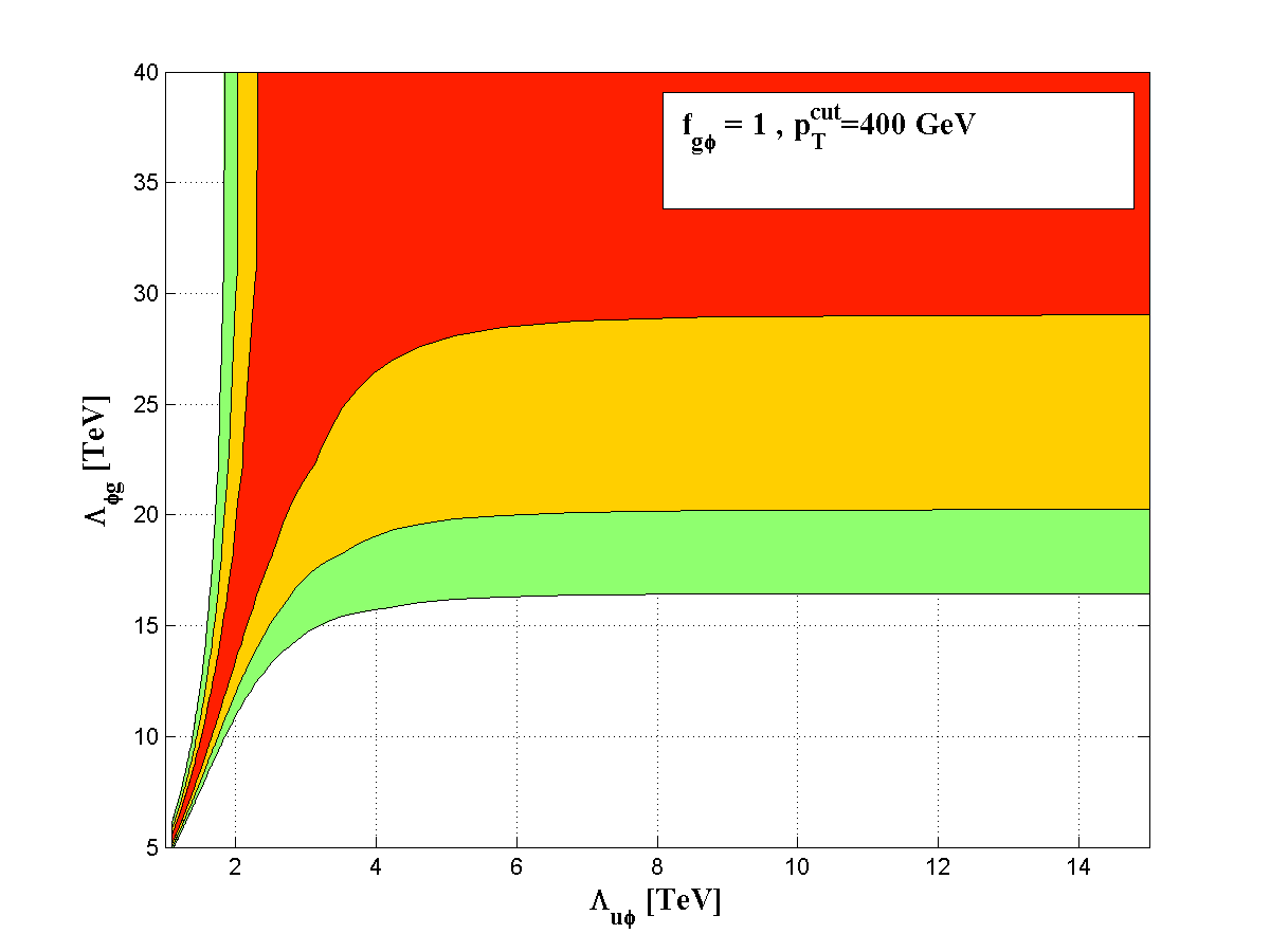
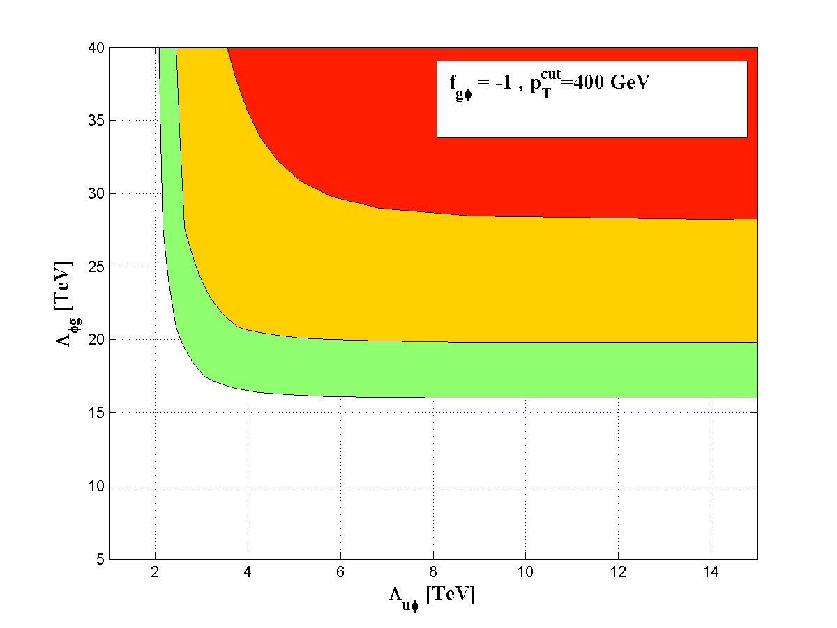
Figure 10: The 68%(red), 95%(orange) and 99%(green) CL ranges in the $\Lambda_{q\phi}-\Lambda_{\phi g}$ plane, corresponding to $\Delta\mu_{hj}^{f}\equiv\left|\mu_{hj}^{f}-1\right|\leq 0.05,~{}0.1$ and $0.15$, respectively, with $p_{T}^{cut}=400$ GeV and for $f_{\phi g}=1$ (upper plot) and $f_{\phi g}=-1$ (lower plot). In both cases $|f_{u\phi}|=1$, see text.

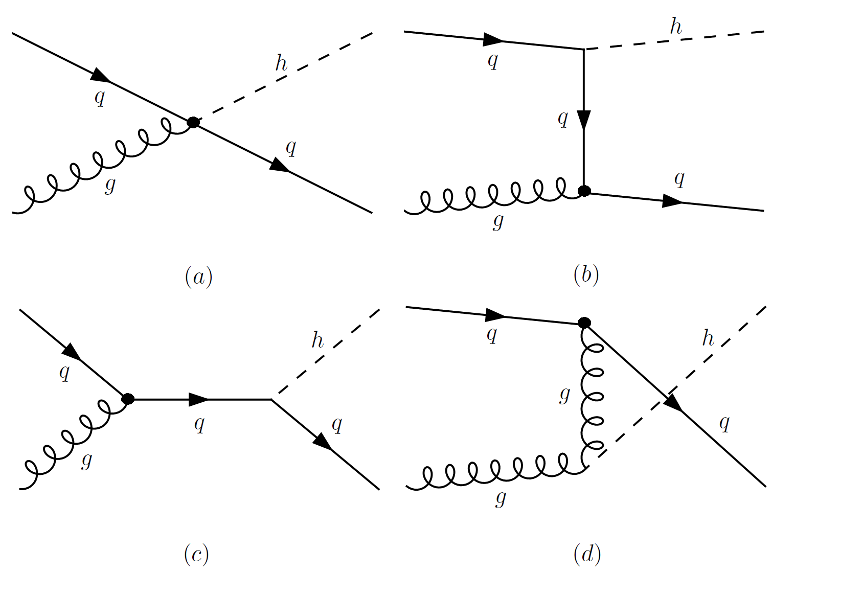
Figure 11: Sample of tree-level diagrams for $gq\to hq$, $q=u,d,c,s,b$ generated by the CMDM-like effective operator ${\cal O}_{qg}$, where the heavy dot represents the CMDM-like vertices. There are additional diagrams for the subprocess $q\bar{q}\to hg$ and $g\bar{q}\to h\bar{q}$ that can also be obtained by crossing symmetry. In the case of a Higgs + light jet production, $pp\to h+j$, diagrams (b) and (c) are essentially absent (i.e., $y_{q}\to 0$).

IV.1 The case of Higgs + light-jet production

Let us consider first the operators ${\cal O}_{u\phi}$ and ${\cal O}_{\phi g}$, which, as seen from Eq. 38, modify the SM $uuh$ and $ggh$ couplings in a way that is equivalent to the kappa-framework (we will focus below only on the case of the 1st generation u-quark operator ${\cal O}_{u\phi}$).^[3] In particular, using Eq. 38 and the analysis performed in the previous section for NP in the kappa-framework, we plot in Fig. 10 the 68%, 95% and 99% CL sensitivity ranges in the $\Lambda_{u\phi}-\Lambda_{\phi g}$ plane, for $p_{T}^{cut}=400$ GeV, assuming that $\mu_{hj}^{f}\sim 1\pm 0.05(1\sigma)$. The sensitivity ranges are shown for the two cases $f_{\phi g}=\pm 1$, where in both cases we set $|f_{u\phi}|=1$, since the cross-section is $\propto\kappa_{q}^{2}$ (see Eq. 19) so that there is no dependence on the sign of $f_{u\phi}$ for $y_{u}^{SM}/y_{b}^{SM}\to 0$ (see Eq. 38).

We see that a measured value of $\mu_{hj}^{f}$ which is consistent with the SM at $3\sigma$ (i.e, with $0.85\leq\mu_{hj}^{f}\leq 1.15$) will exclude NP with typical scales of $\Lambda_{\phi g}\>\raisebox{-2.15277pt}{$\stackrel{{\scriptstyle\textstyle<}}{{\sim}}$}\>15$ TeV (equivalent to $\kappa_{u}\>\raisebox{-2.15277pt}{$\stackrel{{\scriptstyle\textstyle>}}{{\sim}}$}\>0.6$) and $\Lambda_{u\phi}\>\raisebox{-2.15277pt}{$\stackrel{{\scriptstyle\textstyle<}}{{\sim}}$}\>2$ TeV (equivalent to $\kappa_{g}\>\raisebox{-2.15277pt}{$\stackrel{{\scriptstyle\textstyle>}}{{\sim}}$}\>1.1$), for $f_{\phi g}=-1$. In the case of $f_{\phi g}=1$, there is an allowed narrow band in the $\Lambda_{u\phi}-\Lambda_{\phi g}$ plane, stretching down to NP scales of $\Lambda_{\phi g}\sim 5$ TeV and $\Lambda_{u\phi}\sim 1$ TeV, which are consistent with $0.85\leq\mu_{hj}^{f}\leq 1.15$. We note that, as in the kappa-framework analysis, these sensitivity ranges in the $\Lambda_{u\phi}-\Lambda_{\phi g}$ plane mildly depend on the calculation scheme of the SM-like diagrams involving the $ggh$ interaction, i.e., on the difference between the point-like $ggh$ approximation and the exact 1-loop results.

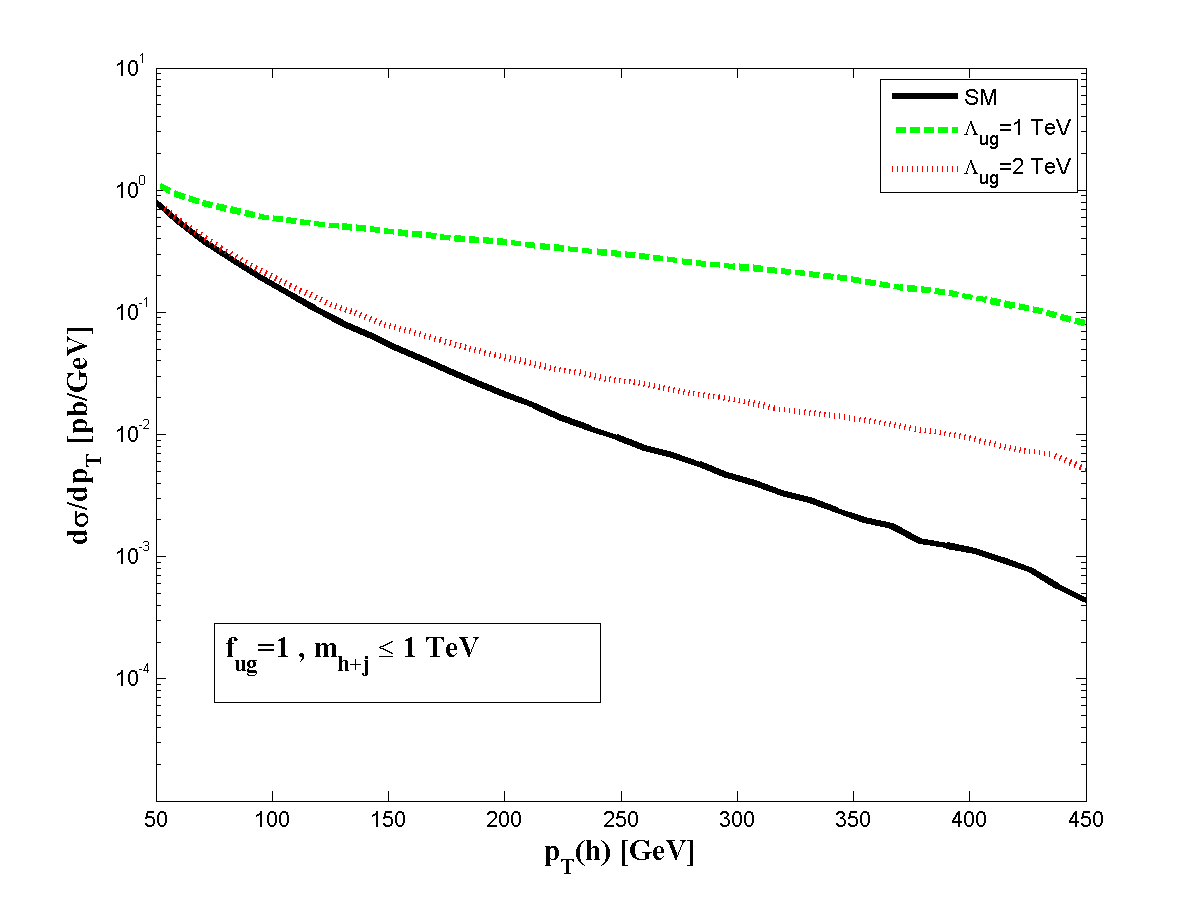
Figure 12: The differential $p_{T}(h)$ distribution, $d\sigma(pp\to h+j)/dp_{T}(h)$, in the SM and with NP in the form of ${\cal O}_{ug}$, for $\Lambda_{ug}=1$ and 2 TeV with $f_{ug}=1$ and with an invariant mass cut of $m_{h+j}\leq 1$ TeV. The SM curve was obtained using the point-like $ggh$ approximation which, as mentioned earlier, overestimates the SM cross-section for $p_{T}(h)\>\raisebox{-2.15277pt}{$\stackrel{{\scriptstyle\textstyle>}}{{\sim}}$}\>200$ GeV.

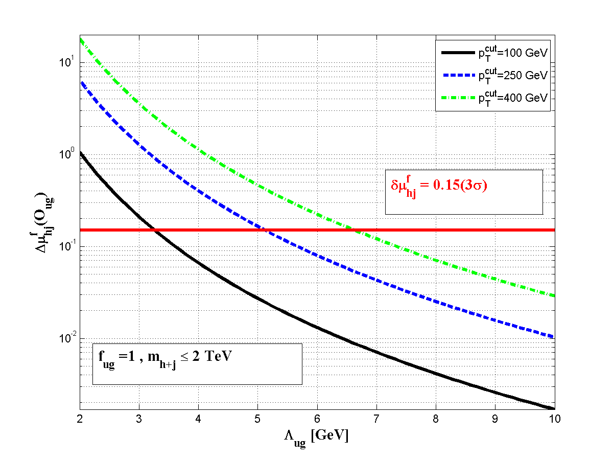
Figure 13: The NP signal $\Delta\mu_{hj}^{f}({\cal O}_{ug})$, as a function of $\Lambda_{ug}$ for $f_{ug}=1$, $p_{T}^{cut}=100,~{}250,~{}400$ GeV and an invariant mass cut of $m_{h+j}\leq 2$ TeV. The horizontal red line indicates the $5\%$ accuracy level. See also text.

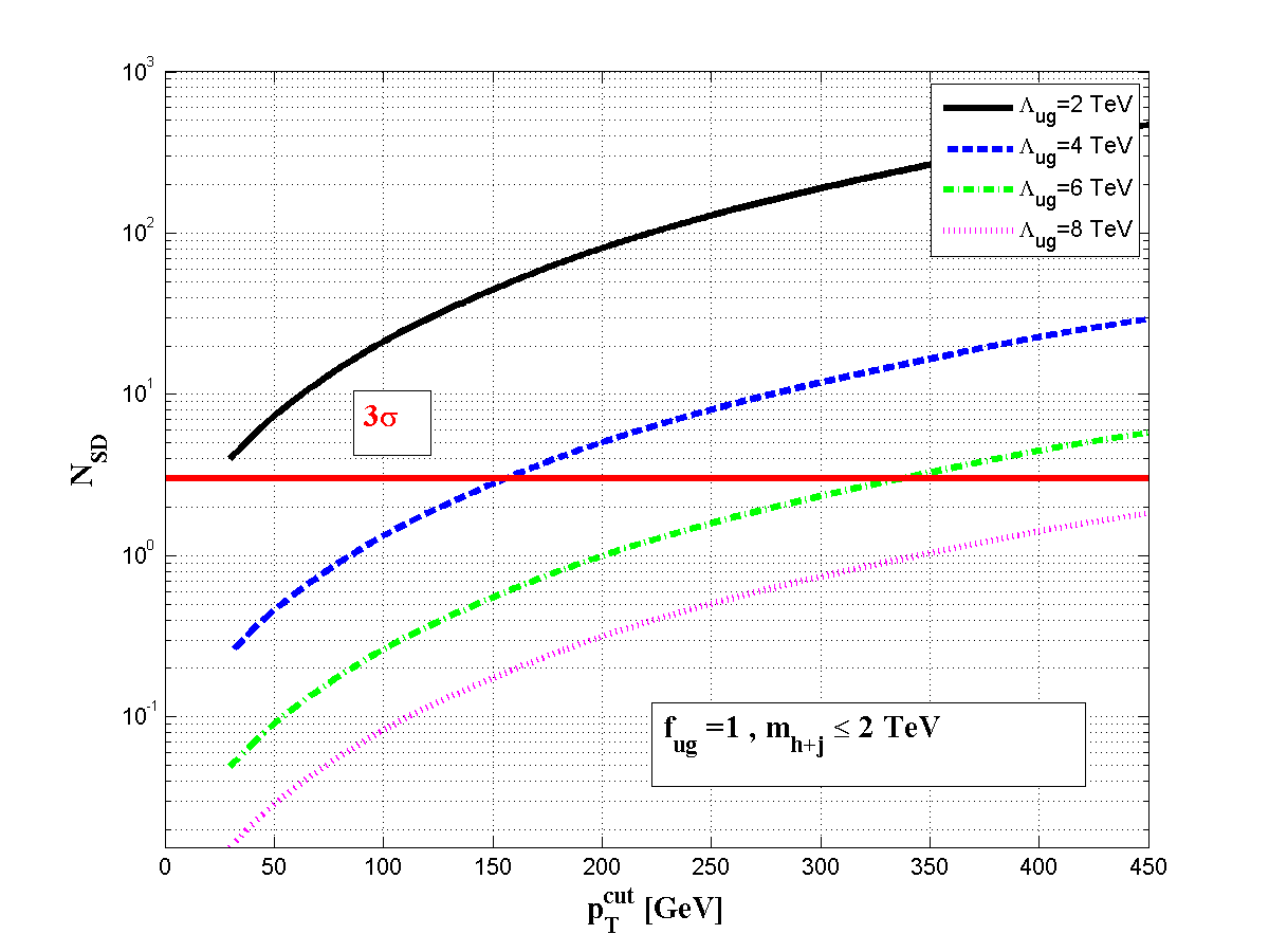
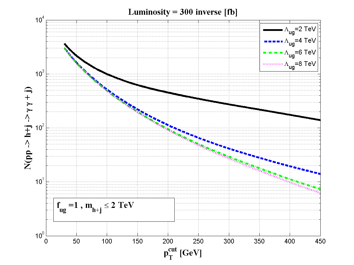
Figure 14: The statistical significance of the signal (upper plot), $N_{SD}=\mu_{hj}^{f}/\delta\mu_{hj}^{f}$, for $\delta\mu_{hj}^{f}=0.05(1\sigma)$, and the expected number of $pp\to h+j\to\gamma\gamma+j$ events (lower plot), as a function of $p_{T}^{cut}$, for $\Lambda_{ug}=2,~{}4,~{}6$ and 8 TeV with $f_{ug}=1$ and with ${\cal L}=300$ fb^-1, a signal acceptance of 50% and an invariant mass cut of $m_{h+j}\leq 2$ TeV. See also text.

We study next the effect of the CMDM-like operator ${\cal O}_{ug}$ on $pp\to h+j$ (again focusing only on the u-quark operator). The tree-level diagrams corresponding to the contribution of ${\cal O}_{ug}$ to $pp\to h+j$ are depicted in Fig. 11. They contain the momentum dependent CMDM-like $uug$ vertex and $uugh$ contact interaction, which do not interfere with the SM diagrams in the limit of $m_{u}\to 0$. In particular, in the presence of ${\cal O}_{ug}$, the total $pp\to h+j$ cross-section can be written as:

$$\sigma^{hj}=\sigma_{SM}^{hj}+\left(\frac{f_{ug}}{\Lambda_{ug}^{2}}\right)^{2}\sigma_{ug}^{hj}~{},$$ (41)

where the squared amplitudes for $\sigma_{SM}^{hj}$ are given in Eqs. 6-8 (see also Eq. 18) and $\sigma_{ug}^{hj}$ is the NP cross-section corresponding to the square of the CMDM-like amplitude, which is generated by the tree-level diagrams for $q\bar{q}\to gh,~{}qg\to qh$ and $\bar{q}g\to\bar{q}h$ shown in Fig. 11, with an insertion of the effective CMDM-like $uug$ and $uugh$ vertices. In particular, $\sigma_{ug}^{hj}$ is composed of $\sigma_{ug}^{hj}=\sigma_{ug}^{hj}\left(q\bar{q}\to gh\right)+\sigma_{ug}^{hj}\left(qg\to qh\right)+\sigma_{ug}^{hj}\left(\bar{q}g\to\bar{q}h\right)$, where the corresponding amplitude squared (summed and averaged over spins and colors) are given by:

$$\sum\overline{\left|{\cal M}_{ug}^{q\bar{q}\to gh}\right|^{2}} = \frac{8}{{\cal C}_{qq}}\hat{u}\hat{t}\left[1-4vC_{g}+8v^{2}C_{g}^{2}\right]~{},$$ (42)

$$\sum\overline{\left|{\cal M}_{ug}^{qg\to qh}\right|^{2}} = -\frac{{\cal C}_{qq}}{{\cal C}_{qg}}\sum\overline{\left|{\cal M}_{ug}^{q\bar{q}\to gh}\right|^{2}}(\hat{s}\leftrightarrow\hat{t})~{},$$ (43)

$$\sum\overline{\left|{\cal M}_{ug}^{\bar{q}g\to\bar{q}h}\right|^{2}} = -\frac{{\cal C}_{qq}}{{\cal C}_{qg}}\sum\overline{\left|{\cal M}_{ug}^{q\bar{q}\to gh}\right|^{2}}(\hat{s}\leftrightarrow\hat{u})~{},$$ (44)

with $\hat{s}=(p_{1}+p_{2})^{2},~{}\hat{t}=(p_{1}+p_{3})^{2}$ and $\hat{u}=(p_{2}+p_{3})^{2}$, defined for $q(-p_{1})+\bar{q}(-p_{2})\to h+g(p_{3})$.

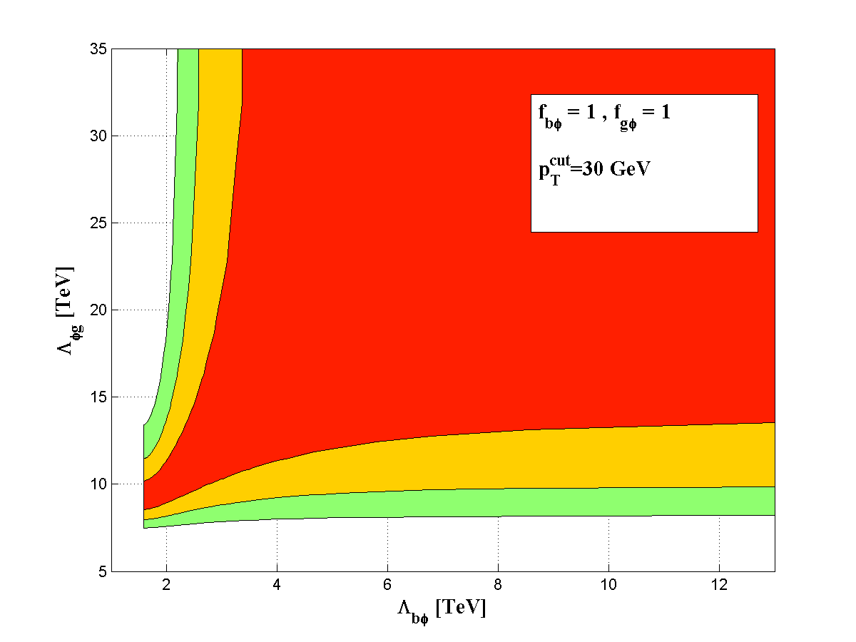
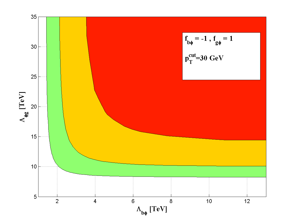
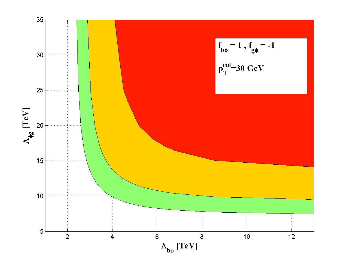
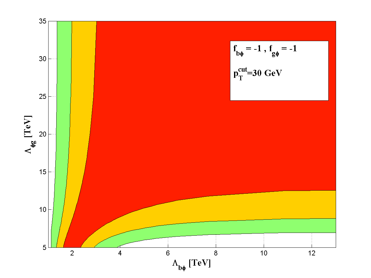
Figure 15: The 68%(red), 95%(orange) and 99%(green) CL sensitivity ranges in the $\Lambda_{b\phi}-\Lambda_{\phi g}$ plane, corresponding to $\Delta\mu_{hj}^{f}\equiv\left|\mu_{hj}^{f}-1\right|\leq 0.05,~{}0.1$ and $0.15$, respectively, with $p_{T}^{cut}=30$ GeV and for $f_{b\phi}=1,~{}f_{\phi g}=1$, $f_{b\phi}=-1,~{}f_{\phi g}=1$, $f_{b\phi}=1,~{}f_{\phi g}=-1$ and $f_{b\phi}=-1,~{}f_{\phi g}=-1$, as indicated in the figures.

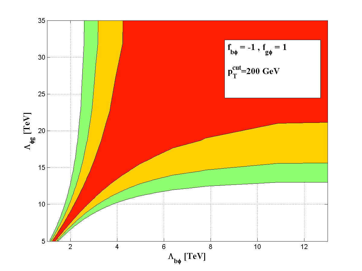
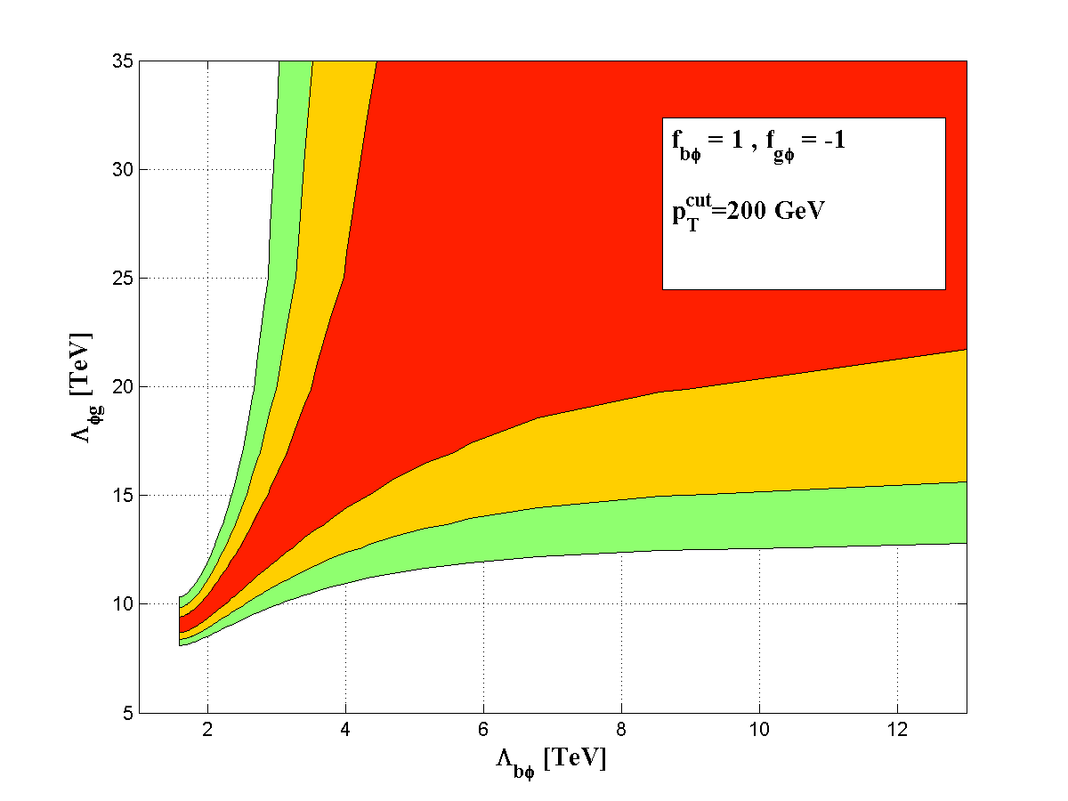
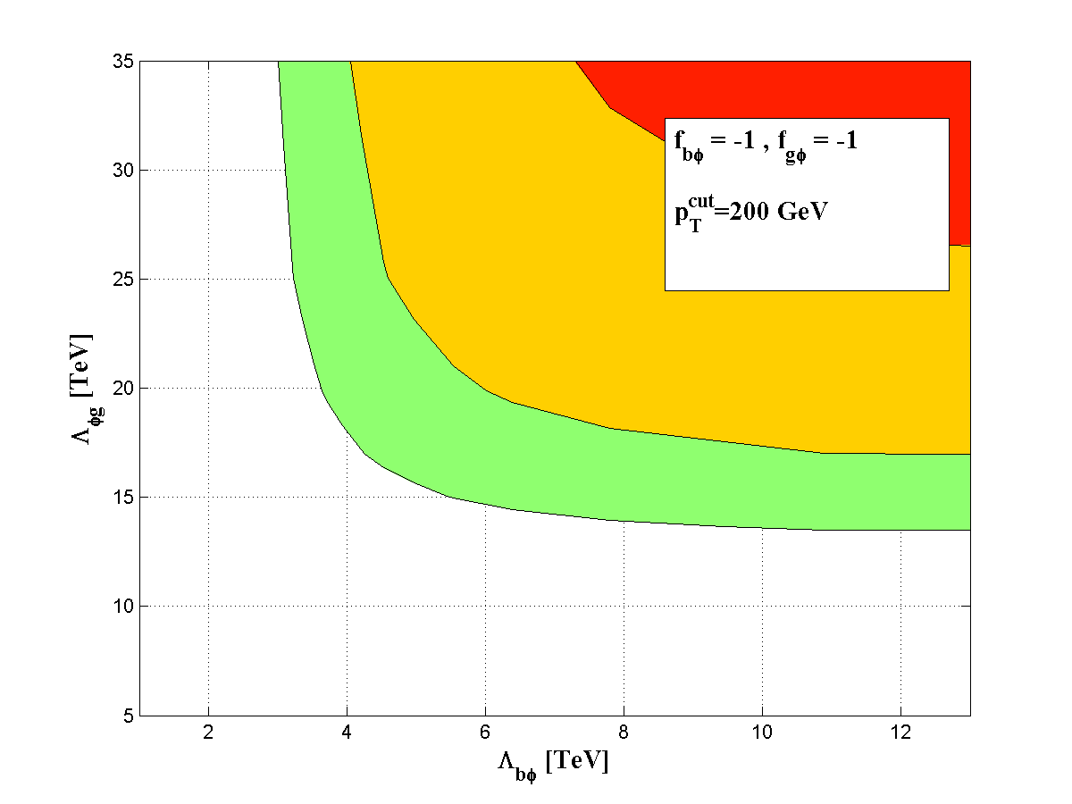
Figure 16: Same as Fig. 15 for $p_{T}^{cut}=200$ GeV.

As illustrated in Fig. 12, the momentum dependent contribution from ${\cal O}_{ug}$ drastically changes the $p_{T}(h)$-dependence of the cross-section with respect to the SM and also with respect to the case where the NP is in the form of scaled couplings (i.e., in the kappa-framework). Indeed, the effect of ${\cal O}_{ug}$ (or any other NP with a similar $p_{T}(h)$ behaviour) are better isolated in the harder Higgs $p_{T}$ regime. This can be obtained by using a relatively high $p_{T}^{cut}$ for the cumulative cross-section (see below).

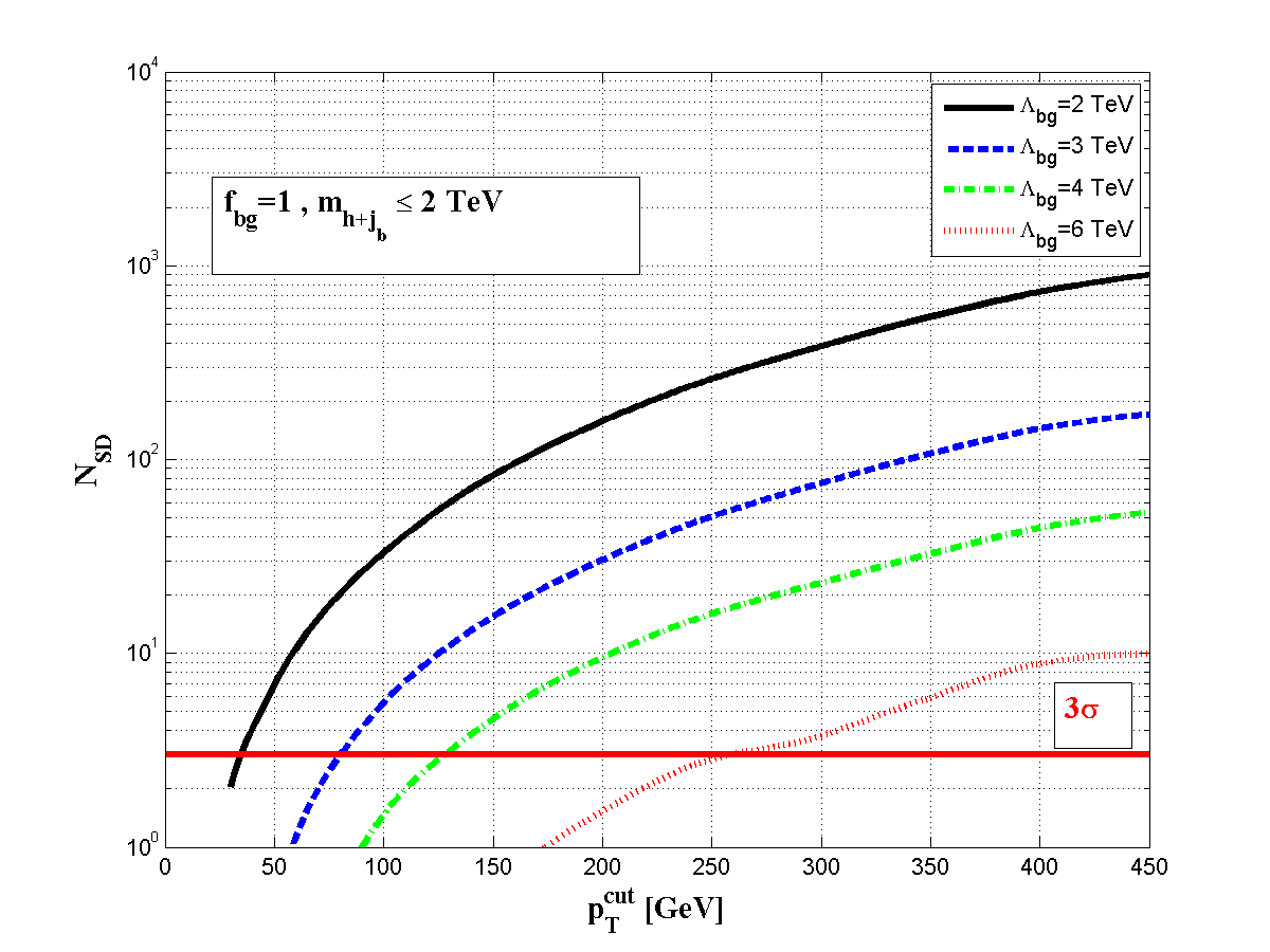
Figure 17: The statistical significance of the signal, $N_{SD}=\mu_{hj_{b}}^{f}/\delta\mu_{hj_{b}}^{f}$, for $\delta\mu_{hj_{b}}^{f}=0.05(1\sigma)$, as a function of $p_{T}^{cut}$, in the presence of ${\cal O}_{bg}$ (assuming no additional NP in the decay) for $f_{bg}=1$ and $\Lambda_{bg}=2,~{}3,~{}4$ and 6 TeV and with an invariant $h+j_{b}$ mass cut of $m_{h+j_{b}}\leq 2$ TeV.

Assuming no additional NP in the decay (the effects of ${\cal O}_{ug}$ in the Higgs decay is $\propto(m_{h}/\Lambda_{ug})^{4}$ and is, therefore, negligible for $\Lambda\sim{\rm few}$ TeV), the corresponding signal strength is:

$$\mu_{hj}^{f}({\cal O}_{ug})=1+\left(\frac{f_{ug}}{\Lambda_{ug}^{2}}\right)^{2}R_{ug}^{hj}~{}~{},~{}~{}R_{ug}^{hj}\equiv\frac{\sigma_{ug}^{hj}}{\sigma_{SM}^{hj}}~{},$$ (45)

so that the NP signal, as defined in Eq. 12, is:

$$\Delta\mu_{hj}^{f}({\cal O}_{ug})=\mid\mu_{hj}^{f}({\cal O}_{ug})-1\mid=\left(\frac{f_{ug}}{\Lambda_{ug}^{2}}\right)^{2}R_{ug}^{hj}~{}.$$ (46)

In Fig. 13 we plot the NP signal, $\Delta\mu_{hj}^{f}({\cal O}_{ug})$, as a function of $\Lambda_{ug}$ with $f_{ug}=1$, for $p_{T}^{cut}$ values of 100, 250 and 400 GeV and an invariant mass cut $m_{h+j}\leq 2$ TeV. As expected (see Fig. 12), the sensitivity to $\Lambda_{ug}$ is significantly improved the higher the $p_{T}^{cut}$ is. In particular, while $\Delta\mu_{hj}^{f}/\mu_{hj}^{f}\>\raisebox{-2.15277pt}{$\stackrel{{\scriptstyle\textstyle>}}{{\sim}}$}\>5\%$ for $p_{T}^{cut}=100$ GeV and $\Lambda_{ug}\>\raisebox{-2.15277pt}{$\stackrel{{\scriptstyle\textstyle<}}{{\sim}}$}\>4$ TeV, for $p_{T}^{cut}=400$ GeV we obtain $\Delta\mu_{hj}^{f}/\mu_{hj}^{f}\>\raisebox{-2.15277pt}{$\stackrel{{\scriptstyle\textstyle>}}{{\sim}}$}\>5\%$ for $\Lambda_{ug}\>\raisebox{-2.15277pt}{$\stackrel{{\scriptstyle\textstyle<}}{{\sim}}$}\>8.5$ TeV.

In Fig. 14 we plot the statistical significance of the signal, $N_{SD}=\mu_{hj}^{f}/\delta\mu_{hj}^{f}$, for $\delta\mu_{hj}^{f}=0.05(1\sigma)$, and the expected number of events, again assuming that the Higgs decays via $h\to\gamma\gamma$, i.e., $N(pp\to h+j\to\gamma\gamma+j)$, as a function of $p_{T}^{cut}$ and for $\Lambda_{ug}=2,~{}4,~{}6$ and 8 TeV with $f_{ug}=1$ and an invariant mass cut $m_{h+j}\leq 2$ TeV. $N(pp\to h+j\to\gamma\gamma+j)$ is shown for an integrated luminosity of 300 fb^-1 and a signal acceptance of 50%. We see, for example, that if $\Lambda_{ug}=6$ TeV, then a high $p_{T}^{cut}\sim 350$ GeV is required in order to obtain a $3\sigma$ effect, for which $N(pp\to h+j\to\gamma\gamma+j)\sim{\cal O}(10)$ and ${\cal O}(100)$ is expected at the LHC with ${\cal L}=300$ fb^-1 and the HL-LHC with ${\cal L}=3000$ fb^-1, respectively.

Note that the effect of changing the calculation scheme of the SM cross-section from the point-like $ggh$ interaction to the exact mass dependent 1-loop one is to change $R_{ug}^{hj}\to r_{ggh}R_{ug}^{hj}$ in Eq. 45 ($r_{ggh}$ is defined in Eq. 15) and therefore it also increases the statistical significance $N_{SD}$ by a factor of $r_{ggh}$ which depends on the $p_{T}^{cut}$ used (see Fig. 3). Thus, the statistical significance values reported in the upper plot of Fig. 14 are on the conservative side.

IV.2 The case of Higgs + b-jet production

As mentioned above, the effects of the NP operators ${\cal O}_{b\phi}$ and ${\cal O}_{\phi g}$ in $pp\to h+j_{b}$, can be described using the kappa-framework formalism of Eq. 16, with the NP factors multiplying the SM $bbh$ Yukawa coupling ($\kappa_{b}$) and $ggh$ coupling ($\kappa_{g}$) as prescribed in Eq. 38.

In Figs. 15 and 16 we plot the 68%, 95% and 99% CL sensitivity ranges in the $\Lambda_{b\phi}-\Lambda_{\phi g}$ plane, for $(f_{b\phi},f_{\phi g})=(1,1),(1,-1),(-1,1),(-1,-1)$ and $p_{T}^{cut}=30$ GeV and 200 GeV, assuming again that the signal strength had been measured to a $5\%(1\sigma)$ accuracy with a SM central value, i.e., $\mu_{hj}^{f}\sim 1\pm 0.05(1\sigma)$. As in the kappa-framework analysis of the previous section, we use the two $p_{T}^{cut}$ values, $p_{T}^{cut}=30$ GeV and $p_{T}^{cut}=200$ GeV, as two representative examples of a high and low statistics $pp\to h+j_{b}\to\gamma\gamma+j_{b}$ signal at the HL-LHC (see also Fig. 7). As expected, a better sensitivity to the NP is obtained for the higher $p_{T}^{cut}=200$ GeV, where $\Lambda_{b\phi}\>\raisebox{-2.15277pt}{$\stackrel{{\scriptstyle\textstyle<}}{{\sim}}$}\>3$ TeV and $\Lambda_{\phi g}\>\raisebox{-2.15277pt}{$\stackrel{{\scriptstyle\textstyle<}}{{\sim}}$}\>{\cal O}(10)$ TeV can be excluded at $3\sigma$ if $\mu_{hj_{b}}^{f}$ is found to be consistent with the SM within 15% ($3\sigma$). Here also, similar to the kappa-framework analysis for $pp\to h+j_{b}$, the sensitivity ranges in the $\Lambda_{b\phi}-\Lambda_{\phi g}$ plane for the $p_{T}^{cut}=200$ GeV case mildly depend on whether the SM cross-section is calculated with the point-like $ggh$ approximation or at 1-loop with a finite top-quark mass.

Finally, we consider the case where the NP in $pp\to h+j_{b}$ is due only to the b-quark CMDM-like operator ${\cal O}_{bg}$. The corresponding tree-level diagrams with the new momentum dependent CMDM-like $bbg$ vertex and $bbgh$ contact interaction are shown in Fig. 11, where, as opposed to the $pp\to h+j$ case, here there is an interference (though small - see below) between the CMDM-like diagrams and the tree-level SM ones (depicted in Fig. 1). In particular, in the presence of ${\cal O}_{bg}$, the total $pp\to h+j_{b}$ cross-section can be written as:

$$\sigma^{hj_{b}}=\sigma_{SM}^{hj_{b}}+\frac{f_{bg}}{\Lambda_{bg}^{2}}\sigma_{bg}^{1,hj_{b}}+\left(\frac{f_{bg}}{\Lambda_{bg}^{2}}\right)^{2}\sigma_{bg}^{2,hj_{b}}~{},$$ (47)

where $\sigma_{SM}^{hj_{b}}$ is the SM cross-section (the relevant SM squared amplitude terms are given in Eqs. 2,3,7,8) and the NP terms $\sigma_{bg}^{1,2}$ can be obtained from the following CMDM-like NP squared amplitudes (summed and averaged over spins and colors):

$$\sum\overline{\left|{\cal M}_{bg}^{1,bg\to bh}\right|^{2}} = \frac{8g_{s}y_{b}}{{\cal C}_{qg}}\left(4vC_{g}\hat{t}-m_{h}^{2}\right)~{},$$ (48)

$$\sum\overline{\left|{\cal M}_{bg}^{2,bg\to bh}\right|^{2}} = -\frac{8}{{\cal C}_{qg}}\left[\hat{s}\hat{u}\left(1-4vC_{g}+8v^{2}C_{g}^{2}\right)\right.$$ (49)

$$\left.+y_{b}^{2}v^{2}\hat{t}\right]~{},$$

$$\sum\overline{\left|{\cal M}_{bg}^{1,\bar{b}g\to\bar{b}h}\right|^{2}} = \sum\overline{\left|{\cal M}_{bg}^{1,bg\to bh}\right|^{2}}(\hat{u}\leftrightarrow\hat{t})~{},$$ (50)

$$\sum\overline{\left|{\cal M}_{bg}^{2,\bar{b}g\to\bar{b}h}\right|^{2}} = \sum\overline{\left|{\cal M}_{bg}^{2,bg\to bh}\right|^{2}}(\hat{u}\leftrightarrow\hat{t})~{},$$ (51)

where again $\hat{s}=(p_{1}+p_{2})^{2},~{}\hat{t}=(p_{1}+p_{3})^{2}$ and $\hat{u}=(p_{2}+p_{3})^{2}$, defined for $b(-p_{1})+\bar{b}(-p_{2})\to h+g(p_{3})$.

We see from Eqs. 48 and 50 above that the interference terms ${\cal M}_{bg}^{1,bg\to bh}$ and ${\cal M}_{bg}^{1,\bar{b}g\to\bar{b}h}$ (corresponding to $\sigma_{bg}^{1,hj_{b}}$ in Eq. 47) are proportional to $y_{b}\sim{\cal O}(m_{b}/v)$ and are therefore sub-leading, so that the dependence of the $pp\to h+j_{b}$ cross-section on the sign of the CMDM-like Wilson coefficient, $f_{bg}$, is tenuous. As a result, $\sigma^{hj_{b}}$ has a very similar $p_{T}$-behaviour as the one depicted in Fig. 12 for the $pp\to h+j$ case. In particular, here also, the Higgs $p_{T}$ spectrum becomes appreciably harder with respect to the SM and also with respect to the case of the NP operators ${\cal O}_{b\phi}$ and ${\cal O}_{g\phi}$, due to the momentum-dependent $\sigma_{bg}^{2,hj_{b}}$ term, which corresponds to the square of the b-quark CMDM-like diagrams, generated by the operator ${\cal O}_{bg}$ and depicted in Fig. 11.

In Fig. 17 we plot the statistical significance of the ${\cal O}_{bg}$ signal for $\delta\mu_{hj}^{f}=0.05(1\sigma)$, as a function of $p_{T}^{cut}$ for $f_{bg}=1$ and $\Lambda_{bg}=2,~{}3,~{}4$ and 6 TeV, imposing an invariant mass cut of $m_{h+j_{b}}\leq 2$ TeV. The results for $f_{bg}=-1$ are very similar due to the small interference between the CMDM-like and SM amplitudes (see discussion above). We see that, as expected, the sensitivity to the scale of the CMDM-like operator, $\Lambda_{bg}$, is higher the higher the $p_{T}^{cut}$ is. We find, for example, that the effect of ${\cal O}_{bg}$ with a typical scale of $\Lambda_{bg}\sim 4$ TeV can be probed in $pp\to h+j_{b}\to\gamma\gamma+j_{b}$ to the level of $N_{SD}\sim{\cal O}(10\sigma)$ with $p_{T}^{cut}=200$ GeV. The expected number of $pp\to h+j_{b}\to\gamma\gamma+j_{b}$ events in this case (i.e., for $\Lambda_{bg}\sim 4$ TeV, $p_{T}^{cut}=200$ GeV and an invariant mass cut of $m_{h+j_{b}}\leq 2$ TeV), assuming an integrated luminosity of 3000 fb^-1, a signal acceptance of ${\cal A}=0.5$ and a b-jet tagging efficiency of 70%, $\epsilon_{b}=0.7$, is $N(pp\to h+j_{b}\to\gamma\gamma+j_{b})\sim 30$ (see also Fig. 7).

As for the sensitivity of the above results to the calculational scheme: due to the smallness of the interference term it is similar to that of the u-quark CMDM-like case in $pp\to h+j$. In particular, the statistical significance $N_{SD}$ shown in Fig. 17 should also be considered conservative with respect to the values which would have been obtained using the exact 1-loop induced SM cross-section, i.e., $N_{SD}$ is naively larger by a factor of $r_{ggh}$ in the exact 1-loop calculation case.

V Summary

We have examined the effects of various NP scenarios, which entail new forms of effective $qqh$ and $qqg$ interactions in conjunction with beyond the SM Higgs-gluon effective coupling, in exclusive Higgs + light-jet ($pp\to h+j$) and Higgs + b-jet ($pp\to h+j_{b}$) production at the LHC. We have defined the signal strength for $pp\to h+j(j_{b})$ followed by the Higgs decay $h\to ff$, as the ratio of the corresponding NP and SM rates, and studied its dependence on the Higgs $p_{T}$ spectrum. We specifically focused on $h\to\gamma\gamma$ and assumed that there is no NP in this decay channel.

We first analyse NP in $pp\to h+j(j_{b})\to\gamma\gamma+j(j_{b})$ within the kappa-framework, in which the SM Higgs couplings to the light-quarks ($qqh$) and to the gluons ($ggh$) are assumed to be scaled by a factor of $\kappa_{q}$ and $\kappa_{g}$, respectively. In particular, in our notation the scale factors $\kappa_{q}$ for all light-quark’s Yukawa couplings ($q=u,d,c,s,b$) are normalized with respect to the b-quark Yukawa, $\kappa_{q}=y_{q}/y_{b}^{SM}$, so that in the SM we have e.g., $\kappa_{b}=1$ and $\kappa_{u}\sim{\cal O}(10^{-3})$. This NP setup does not introduce any new Lorentz structure in the underlying hard processes (i.e., $gg\to gh$, $qg\to qh$, $\bar{q}g\to\bar{q}h$, $q\bar{q}\to gh$ in the case of $pp\to h+j$ and $bg\to bh$, $\bar{b}g\to\bar{b}h$ in the case of $pp\to h+j_{b}$), thus retaining the SM $pp\to h+j(j_{b})$ kinematics. In particular, we find that strong bounds can be obtained in the $\kappa_{g}-\kappa_{q}$ plane at the LHC, by measuring a $p_{T}$-dependent signal strength for Higgs + jet events at relatively high Higgs $p_{T}$. For example, the combination of $\kappa_{g}<0.8$ with $\kappa_{u}>0.25$ ($\kappa_{g}<0.8$ with $\kappa_{b}>1.5$) can be excluded at more than $7\sigma$ at the HL-LHC with a luminosity of 3000 fb^-1, if the signal strength in the $pp\to h+j(j_{b})\to\gamma\gamma+j(j_{b})$ channels will be measured and known to an accuracy of $5\%(1\sigma)$, for high $p_{T}(h)$ events with $p_{T}(h)\geq 400(200)$ GeV. Recall that in our notation the corresponding SM strengths of these couplings are $\kappa_{b}=\kappa_{g}=1$ and $\kappa_{u}\sim{\cal O}(10^{-3})$.

We also considered NP effects in $pp\to h+j(j_{b})$ in the SMEFT framework, where higher dimensional effective operators modify the SM $qqh$ Yukawa couplings and the Higgs-gluon $ggh$ interaction by a scaling factor, similar to the case of the kappa-framework for NP. We thus utilize an interesting “mapping” between the SMEFT and kappa-frameworks to derive new bounds on the typical scale of NP that underlies the SMEFT lagrangian. We find, for example, that $pp\to h+j(j_{b})\to\gamma\gamma+j(j_{b})$ events with high $p_{T}(h)>400(200)$ GeV at the HL-LHC, are sensitive to the new effective operators that modify the $qqh$ (Yukawa) and $ggh$ couplings, if their typical scale (i.e., with ${\cal O}(1)$ dimensionless Wilson coefficients) is a few TeV and ${\cal O}(10)$ TeV, respectively.

Finally, as a counter example, we study the effects of NP in the form of dimension six u-quark and b-quark chromo magnetic dipole moment (CMDM)-like effective operators, which induce new derivative and new contact interactions that significantly distort the $pp\to h+j(j_{b})$ SM kinematics and, therefore, cannot be described in terms of scaled couplings. In particular, in this case, the high-$p_{T}$ Higgs spectrum becomes significantly harder with respect to the SM. We thus show that $pp\to h+j(j_{b})\to\gamma\gamma+j(j_{b})$ events at the HL-LHC, with a high Higgs $p_{T}$ of $p_{T}(h)\>\raisebox{-2.15277pt}{$\stackrel{{\scriptstyle\textstyle>}}{{\sim}}$}\>400(200)$ GeV, can probe the higher dimensional CMDM-like u-quark and b-quark effective operators, if their typical scale is around $\Lambda\sim 5$ TeV.

Our main results were obtained using an effective point-like $ggh$ interaction approximation. To estimate the sensitivity to this approximation, we also compared samples of our results to the case where the $ggh$ vertex is calculated explicitly at leading order, which, for Higgs + jet, corresponds to a 1-loop mass dependent calculation using a finite top-quark mass.

Acknowledgments: The work of AS was supported in part by the US DOE contract #DE-SC0012704.

References

- (1) G. Aad et al., the ATLAS collaboration, JHEP 1409 (2014), 112, arXiv:1407.4222 [hep-ex].
- (2) G. Aad et al., the ATLAS collaboration, Phys.Lett. B738 (2014), 234, arXiv:1408.3226 [hep-ex].
- (3) G. Aad et al., the ATLAS collaboration, Phys.Rev.Lett. 115 (2015) no.9, 091801, arXiv:1504.05833 [hep-ex].
- (4) G. Aad et al., the ATLAS collaboration, JHEP 1608 (2016), 104, arXiv:1604.02997 [hep-ex].
- (5) V. Khachatryan et al., the CMS collaboration, Eur.Phys. J. C76 (2016), 13, arXiv:1508.07819 [hep-ex].
- (6) V. Khachatryan et al., the CMS collaboration, arXiv:1606.01522 [hep-ex].
- (7) X. Chen, J. Cruz-Martinez, T. Gehrmann, E.W.N. Glover, M. Jaquier, JHEP 1610 (2016), 066, arXiv:1607.08817 [hep-ph].
- (8) R. Boughezal, F. Caola, K. Melnikov, F. Petriello, M. Schulze, JHEP 1306 (2013), 072, Phys.Rev.Lett. 115 (2015) no.8, 082003, arXiv:1504.07922 [hep-ph].
- (9) F. Caola, K. Melnikov, M. Schulze, JHEP 1306 (2013), 072, Phys.Rev. D92 (2015) no.7, 074032, arXiv:1508.02684 [hep-ph].
- (10) X. Chen, T. Gehrmann, E.W.N. Glover, M. Jaquier, Phys.Lett. B740 (2015), 147, arXiv:1408.5325 [hep-ph]; ibid. arXiv:1604.04085 [hep-ph].
- (11) R. Boughezal, C. Focke, W. Giele, X. Liu, F. Petriello, Phys.Lett. B748 (2015), 5, arXiv:1505.03893 [hep-ph].
- (12) N. Greiner., S. Hoche, G. Luisoni., M. Schönherr, J.-C. Winter, JHEP 1701 (2017), 091, arXiv:1608.01195 [hep-ph].
- (13) R.V. Harlander, T. Neumann, K.J. Ozeren, M. Wiesemann, JHEP 1208 (2012), 139, arXiv:1206.0157 [hep-ph].
- (14) T. Neumann, C. Williams, Phys.Rev. D95 (2017) no.1, 014004, arXiv:1609.00367 [hep-ph].
- (15) J.M. Lindert, K. Melnikov, L. Tancredi, C. Wever, arXiv:1703.03886 [hep-ph].
- (16) R.K. Ellis, I. Hinchliffe, M. Soldate, J.J. van der Bij, Nucl.Phys. B297 (1988) 221.
- (17) U. Baur, E.W.Nigel Glover, Nucl.Phys. B339 (1990), 38.
- (18) D. de Florian, M. Grazzini, Z. Kunszt, Phys.Rev.Lett. 82 (1999), 5209, hep-ph/9902483.
- (19) V. Ravindran, J. Smith, W.L. Van Neerven, Nucl.Phys. B634 (2002), 247, hep-ph/0201114.
- (20) R. Boughezal, F. Caola, K. Melnikov, F. Petriello, M. Schulze, JHEP 1306 (2013), 072, arXiv:1302.6216 [hep-ph].
- (21) B. Jager, L. Reina, D. Wackeroth, Phys.Rev. D93 (2016) no.1, 014030, arXiv:1509.05843 [hep-ph].
- (22) E. Braaten, H. Zhang, J.-W. Zhang, arXiv:1704.06620 [hep-ph].
- (23) O. Brein, W. Hollik, Phys.Rev. D68 (2003), 095006, hep-ph/0305321.
- (24) S. Dittmaier, Michael Kramer, M. Spira, Phys.Rev. D70 (2004), 074010, e-Print: hep-ph/0309204.
- (25) S. Dawson, C.B. Jackson, L. Reina, D. Wackeroth, Phys.Rev. D69 (2004), 074027, e-Print: hep-ph/0311067; ibid. Phys.Rev.Lett. 94 (2005), 031802, e-Print: hep-ph/0408077; ibid. Mod.Phys.Lett. A21 (2006), 89, e-Print: hep-ph/0508293.
- (26) J.M. Campbell et al., e-Print: hep-ph/0405302.
- (27) A. Banfi, A. Martin, V. Sanz, JHEP 1408 (2014), 053, arXiv:1308.4771 [hep-ph].
- (28) C. Grojean, E. Salvioni, M. Schlaffer, A. Weiler, JHEP 1405 (2014), 022, arXiv:1312.3317 [hep-ph].
- (29) D. Ghosh, M. Wiebusch, Phys.Rev. D91 (2015) no.3, 031701, arXiv:1411.2029 [hep-ph].
- (30) S. Dawson, I.M. Lewis, Mao Zeng, Phys.Rev. D90 (2014) no.9, 093007, arXiv:1409.6299 [hep-ph].
- (31) R. V. Harlander, T. Neumann, Phys.Rev. D88 (2013), 074015, arXiv:1308.2225 [hep-ph].
- (32) J. Bramante, A. Delgado, L. Lehman, A. Martin, Phys.Rev. D93 (2016) no.5, 053001, arXiv:1410.3484 [hep-ph].
- (33) A. Azatov, A. Paul, JHEP 1401 (2014), 014, arXiv:1309.5273 [hep-ph].
- (34) M. Schlaffer, M. Spannowsky, M. Takeuchi, A. Weiler, C. Wymant, Eur.Phys. J. C74 (2014) no.10, 3120, arXiv:1405.4295 [hep-ph].
- (35) M. Buschmann, C. Englert, D. Goncalves, T. Plehn, M. Spannowsky, Phys.Rev. D90 (2014) no.1, 013010, arXiv:1405.7651 [hep-ph].
- (36) M. Grazzini., A. Ilnicka., M. Spira., M. Wiesemann, arXiv:1612.00283 [hep-ph].
- (37) H. Mantler, M. Wiesemann, Eur. Phys. J. C73 (2013), 2467, arXiv:1210.8263 [hep-ph]; M. Grazzini, H. Sargsyan, JHEP 1309 (2013), 129, arXiv:1306.4581 [hep-ph].
- (38) https://cp3.irmp.ucl.ac.be/projects/madgraph/wiki/Models/HiggsEffective#no1.
- (39) A.L. Kagan, G. Perez, F. Petriello, Y. Soreq, S. Stoynev, J. Zupan, Phys.Rev.Lett. 114 (2015), 101802, arXiv:1406.1722 [hep-ph]; G. Perez, Y. Soreq, E. Stamou, K. Tobioka, Phys.Rev. D92 (2015), 033016, arXiv:1503.00290 [hep-ph].
- (40) G. Perez, Y. Soreq, E. Stamou, K. Tobioka1, arXiv:1505.06689 [hep-ph].
- (41) Y. Soreq, H.X. Zhu, J. Zupan, arXiv:1606.09621 [hep-ph].
- (42) F. Bishara, U. Haisch, P.F. Monni, E. Re, Phys.Rev.Lett. 118 (2017), 121801, arXiv:1606.09253 [hep-ph].
- (43) M. Buschmann, D. Goncalves, S. Kuttimalai, M. Schonherr, F. Krauss, T. Plehn, JHEP 1502 (2015), 038, arXiv:1410.5806 [hep-ph]; R. Frederix, S. Frixione, E. Vryonidou, M. Wiesemann, JHEP 1608 (2016), 006, arXiv:1604.03017 [hep-ph].
- (44) G. Bonner, H.E. Logan, arXiv:1608.04376 [hep-ph].
- (45) F. Yu, arXiv:1609.06592 [hep-ph].
- (46) L.M. Carpenter, T. Han, K. Hendricks, Z. Qian, N. Zhouc, Phys.Rev.D95 (2017) no.5, 053003, arXiv:1611.05463 [hep-ph].
- (47) J. Gao, arXiv:1608.01746 [hep-ph].
- (48) J.L. Diaz-Cruz, U.J. Saldaña-Salazar, Nucl.Phys. B913 (2016), 942, arXiv:1405.0990 [hep-ph].
- (49) T. Han, X. Wang, arXiv:1704.00790 [hep-ph].
- (50) J. Alwall, R. Frederix, S. Frixione, V. Hirschi, F. Maltoni, O. Mattelaer, H.S. Shao, T. Stelzer, P. Torrielli, M. Zaro, JHEP 07 (2014), 079, arXiv:1405.0301 [hep-ph].
- (51) A. Alloul et al., Comput.Phys.Commun. 185 (2014), 2250, arXiv:1310.1921 [hep-ph].
- (52) T. Hahn, S. Paßehr, C. Schappacher, PoS LL2016 (2016) 068, [J.Phys.Conf.Ser. 762 (2016) no.1, 012065], arXiv:1604.04611 [hep-ph].
- (53) Vladyslav Shtabovenko. FeynCalc 9. J. Phys. Conf. Ser., 762(1):012064, 2016 V. Shtabovenko, J.Phys.Conf.Ser. 762 (2016) no.1, 012064, arXiv:1604.06709 [hep-ph].
- (54) A.Martin, W. Stirling, R. Thorne, G. Watt, Eur.Phys.J. C63 (2009), 189, arXiv:0901.0002 [hep-ph].
- (55) E. Conte, B. Fuks, G. Serret, Comput.Phys.Commun. 184 (2013) 222, arXiv:1206.1599 [hep-ph].
- (56) See e.g., Working Group Report: Higgs Boson, Sally Dawson et al., arXiv:1310.8361 [hep-ex]; LHC Higgs Cross Section Working Group, S. Heinemeyer et al., arXiv:1101.0593 [hep-ph], S. Dittmaier et al., arXiv:1201.3084 [hep-ph], S. Heinemeyer et al., arXiv:1307.1347 [hep-ph] and D. de Florian et al., arXiv:1610.07922 [hep-ph].
- (57) LHC Higgs Cross Section Working Group Collaboration, A. David et al., arXiv:1209.0040 [hep-ph].
- (58) C. Mariotti, G. Passarino,Int.J.Mod.Phys. A32 (2017) no.04, 1730003, arXiv:1612.00269 [hep-ph].
- (59) M. Wiesemann, R. Frederix, S. Frixione, V. Hirschi, F. Maltoni, P. Torrielli, JHEP 1502 (2015), 132, arXiv:1409.5301 [hep-ph].
- (60) K.J. Ozeren, JHEP 1011 (2010), 084, arXiv:1010.2977 [hep-ph].
- (61) R. V. Harlander, K.J. Ozeren, M. Wiesemann, Phys.Lett. B693 (2010), 269, arXiv:1007.5411 [hep-ph].
- (62) ATLAS and CMS Collaborations (G. Aad et al.), JHEP 1608 (2016), 045, arXiv:1606.02266 [hep-ex].
- (63) W. Buchmiiller, D. Wyler, Nucl. Phys. B268 (1986), 621; C. Arzt, M.B. Einhorn, J. Wudka, Nucl. Phys. B433 (1995), 41; M. B Einhorn and J. Wudka, Nucl. Phys. B876 (2013), 556.
- (64) B. Grzadkowski, M. Iskrzynski, M. Misiak, J. Rosiek, JHEP 1010 (2010), 085.
- (65) A. Hayreter, G. Valencia, Phys.Rev. D88 (2013), 034033, e-Print: arXiv:1304.6976 [hep-ph]; ibid.,arXiv:1411.0035 [hep-ph].