Neural Models for Documents with Metadata

Abstract

Most real-world document collections involve various types of metadata, such as author, source, and date, and yet the most commonly-used approaches to modeling text corpora ignore this information. While specialized models have been developed for particular applications, few are widely used in practice, as customization typically requires derivation of a custom inference algorithm. In this paper, we build on recent advances in variational inference methods and propose a general neural framework, based on topic models, to enable flexible incorporation of metadata and allow for rapid exploration of alternative models. Our approach achieves strong performance, with a manageable tradeoff between perplexity, coherence, and sparsity. Finally, we demonstrate the potential of our framework through an exploration of a corpus of articles about US immigration.

1 Introduction

Topic models comprise a family of methods for uncovering latent structure in text corpora, and are widely used tools in the digital humanities, political science, and other related fields Boyd-Graber et al. (2017). Latent Dirichlet allocation (LDA; Blei et al., 2003) is often used when there is no prior knowledge about a corpus. In the real world, however, most documents have non-textual attributes such as author Rosen-Zvi et al. (2004), timestamp Blei and Lafferty (2006), rating McAuliffe and Blei (2008), or ideology Eisenstein et al. (2011); Nguyen et al. (2015b), which we refer to as metadata.

Many customizations of LDA have been developed to incorporate document metadata. Two models of note are supervised LDA (SLDA; McAuliffe and Blei, 2008), which jointly models words and labels (e.g., ratings) as being generated from a latent representation, and sparse additive generative models (SAGE; Eisenstein et al., 2011), which assumes that observed covariates (e.g., author ideology) have a sparse effect on the relative probabilities of words given topics. The structural topic model (STM; Roberts et al., 2014), which adds correlations between topics to SAGE, is also widely used, but like SAGE it is limited in the types of metadata it can efficiently make use of, and how that metadata is used. Note that in this work we will distinguish labels (metadata that are generated jointly with words from latent topic representations) from covariates (observed metadata that influence the distribution of labels and words).

The ability to create variations of LDA such as those listed above has been limited by the expertise needed to develop custom inference algorithms for each model. As a result, it is rare to see such variations being widely used in practice. In this work, we take advantage of recent advances in variational methods Kingma and Welling (2014); Rezende et al. (2014); Miao et al. (2016); Srivastava and Sutton (2017) to facilitate approximate Bayesian inference without requiring model-specific derivations, and propose a general neural framework for topic models with metadata, scholar.

scholar combines the abilities of SAGE and SLDA, and allows for easy exploration of the following options for customization:

1. Covariates: as in SAGE and STM, we incorporate explicit deviations for observed covariates, as well as effects for interactions with topics.

2. Supervision: as in SLDA, we can use metadata as labels to help infer topics that are relevant in predicting those labels.

3. Rich encoder network: we use the encoding network of a variational autoencoder (VAE) to incorporate additional prior knowledge in the form of word embeddings, and/or to provide interpretable embeddings of covariates.

4. Sparsity: as in SAGE, a sparsity-inducing prior can be used to encourage more interpretable topics, represented as sparse deviations from a background log-frequency.

We begin with the necessary background and motivation (§2), and then describe our basic framework and its extensions (§3), followed by a series of experiments (§4). In an unsupervised setting, we can customize the model to trade off between perplexity, coherence, and sparsity, with improved coherence through the introduction of word vectors. Alternatively, by incorporating metadata we can either learn topics that are more predictive of labels than SLDA, or learn explicit deviations for particular parts of the metadata. Finally, by combining all parts of our model we can meaningfully incorporate metadata in multiple ways, which we demonstrate through an exploration of a corpus of news articles about US immigration.

In presenting this particular model, we emphasize not only its ability to adapt to the characteristics of the data, but the extent to which the VAE approach to inference provides a powerful framework for latent variable modeling that suggests the possibility of many further extensions. Our implementation is available at https://github.com/dallascard/scholar.

2 Background and Motivation

LDA can be understood as a non-negative Bayesian matrix factorization model: the observed document-word frequency matrix, $\mathbf{X}\in\mathbb{Z}^{D\times V}$ ($D$ is the number of documents, $V$ is the vocabulary size) is factored into two low-rank matrices, $\bm{\Theta}^{D\times K}$ and $\mathbf{B}^{K\times V}$, where each row of $\bm{\Theta}$, $\bm{\theta}_{i}\in\Delta^{K}$ is a latent variable representing a distribution over topics in document $i$, and each row of $\mathbf{B}$, $\bm{\beta}_{k}\in\Delta^{V}$, represents a single topic, i.e., a distribution over words in the vocabulary. While it is possible to factor the count data into unconstrained matrices, the particular priors assumed by LDA are important for interpretability Wallach et al. (2009). For example, the neural variational document model (NVDM; Miao et al., 2016) allows $\bm{\theta}_{i}\in\mathbb{R}^{K}$ and achieves normalization by taking the softmax of $\bm{\theta}_{i}^{\top}\mathbf{B}$. However, the experiments in Srivastava and Sutton (2017) found the performance of the NVDM to be slightly worse than LDA in terms of perplexity, and dramatically worse in terms of topic coherence.

The topics discovered by LDA tend to be parsimonious and coherent groupings of words which are readily identifiable to humans as being related to each other Chang et al. (2009), and the resulting mode of the matrix $\bm{\Theta}$ provides a representation of each document which can be treated as a measurement for downstream tasks, such as classification or answering social scientific questions Wallach (2016). LDA does not require — and cannot make use of — additional prior knowledge. As such, the topics that are discovered may bear little connection to metadata of a corpus that is of interest to a researcher, such as sentiment, ideology, or time.

In this paper, we take inspiration from two models which have sought to alleviate this problem. The first, supervised LDA (SLDA; McAuliffe and Blei, 2008), assumes that documents have labels $y$ which are generated conditional on the corresponding latent representation, i.e., ${y}_{i}\sim p({y}\mid\bm{\theta}_{i})$. By incorporating labels into the model, it is forced to learn topics which allow documents to be represented in a way that is useful for the classification task. Such models can be used inductively as text classifiers (Balasubramanyan et al., 2012).

SAGE Eisenstein et al. (2011), by contrast, is an exponential-family model, where the key innovation was to replace topics with sparse deviations from the background log-frequency of words ($\bm{d}$), i.e., $p(\textrm{word}\mid\textrm{softmax}(\bm{d}+\bm{\theta}_{i}^{\top}\mathbf{B}))$. SAGE can also incorporate deviations for observed covariates, as well as interactions between topics and covariates, by including additional terms inside the softmax. In principle, this allows for inferring, for example, the effect on an author’s ideology on their choice of words, as well as ideological variations on each underlying topic. Unlike the NVDM, SAGE still constrains $\bm{\theta}_{i}$ to lie on the simplex, as in LDA.

SLDA and SAGE provide two different ways that users might wish to incorporate prior knowledge as a way of guiding the discovery of topics in a corpus: SLDA incorporates labels through a distribution conditional on topics; SAGE includes explicit sparse deviations for each unique value of a covariate, in addition to topics.

Because of the Dirichlet-multinomial conjugacy in the original model, efficient inference algorithms exist for LDA. Each variation of LDA, however, has required the derivation of a custom inference algorithm, which is a time-consuming and error-prone process. In SLDA, for example, each type of distribution we might assume for $p({y}\mid\bm{\theta})$ would require a modification of the inference algorithm. SAGE breaks conjugacy, and as such, the authors adopted L-BFGS for optimizing the variational bound. Moreover, in order to maintain computational efficiency, it assumed that covariates were limited to a single categorical label.

More recently, the variational autoencoder (VAE) was introduced as a way to perform approximate posterior inference on models with otherwise intractable posteriors Kingma and Welling (2014); Rezende et al. (2014). This approach has previously been applied to models of text by Miao et al. (2016) and Srivastava and Sutton (2017). We build on their work and show how this framework can be adapted to seamlessly incorporate the ideas of both SAGE and SLDA, while allowing for greater flexibility in the use of metadata. Moreover, by exploiting automatic differentiation, we allow for modification of the model without requiring any change to the inference procedure. The result is not only a highly adaptable family of models with scalable inference and efficient prediction; it also points the way to incorporation of many ideas found in the literature, such as a gradual evolution of topics Blei and Lafferty (2006), and hierarchical models Blei et al. (2010); Nguyen et al. (2013, 2015b).

3 scholar: A Neural Topic Model with Covariates, Supervision, and Sparsity

We begin by presenting the generative story for our model, and explain how it generalizes both SLDA and SAGE (§3.1). We then provide a general explanation of inference using VAEs and how it applies to our model (§3.2), as well as how to infer document representations and predict labels at test time (§3.3). Finally, we discuss how we can incorporate additional prior knowledge (§3.4).

3.1 Generative Story

Consider a corpus of $D$ documents, where document $i$ is a list of $N_{i}$ words, $\bm{w}_{i}$, with $V$ words in the vocabulary. For each document, we may have observed covariates $\bm{c}_{i}$ (e.g., year of publication), and/or one or more labels, $\bm{y}_{i}$ (e.g., sentiment).

Our model builds on the generative story of LDA, but optionally incorporates labels and covariates, and replaces the matrix product of $\bm{\Theta}$ and $\mathbf{B}$ with a more flexible generative network, $f_{g}$, followed by a softmax transform. Instead of using a Dirichlet prior as in LDA, we employ a logistic normal prior on $\bm{\theta}$ as in Srivastava and Sutton (2017) to facilitate inference (§3.2): we draw a latent variable, $\bm{r}$, from a multivariate normal, and transform it to lie on the simplex using a softmax transform.

The generative story is shown in Figure 1(a) and described in equations below:

• For each document $i$ of length $N_{i}$:

  • # Draw a latent representation on the simplex from a logistic normal prior:

  • $\bm{r}_{i}\sim\mathcal{N}(\bm{r}\mid\bm{\mu}_{0}(\alpha),\textrm{diag}(\bm{\sigma}^{2}_{0}(\alpha)))$

  • $\bm{\theta}_{i}=\textrm{softmax}(\bm{r}_{i})$

  • # Generate words, incorporating covariates:

  • $\bm{\eta}_{i}=f_{g}(\bm{\theta}_{i},\bm{c}_{i})$

  • For each word $j$ in document $i$:

    • $w_{ij}\sim p({w}\mid\textrm{softmax}(\bm{\eta}_{i}))$

  • # Similarly generate labels:

  • $\bm{y}_{i}\sim p(\bm{y}\mid f_{y}(\bm{\theta}_{i},\bm{c}_{i}))$,

where $p({w}\mid\textrm{softmax}(\bm{\eta}_{i}))$ is a multinomial distribution and $p(\bm{y}\mid f_{y}(\bm{\theta}_{i},\bm{c}_{i}))$ is a distribution appropriate to the data (e.g., multinomial for categorical labels). $f_{g}$ is a model-specific combination of latent variables and covariates, $f_{y}$ is a multi-layer neural network, and $\bm{\mu}_{0}(\alpha)$ and $\bm{\sigma}_{0}^{2}(\alpha)$ are the mean and diagonal covariance terms of a multivariate normal prior. To approximate a symmetric Dirichlet prior with hyperparameter $\alpha$, these are given by the Laplace approximation Hennig et al. (2012) to be $\mu_{0,k}(\alpha)=0$ and $\sigma_{0,k}^{2}=(K-1)/(\alpha K)$.

If we were to ignore covariates, place a Dirichlet prior on $\mathbf{B}$, and let $\bm{\eta}=\bm{\theta}_{i}^{\top}\mathbf{B}$, this model is equivalent to SLDA with a logistic normal prior. Similarly, we can recover a model that is like SAGE, but lacks sparsity, if we ignore labels, and let

$$\bm{\eta}_{i}=\bm{d}+\bm{\theta}_{i}^{\top}\mathbf{B}+\bm{c}_{i}^{\top}\mathbf{B}^{\textit{cov}}+(\bm{\theta}_{i}\otimes\bm{c}_{i})^{\top}\mathbf{B}^{\textit{int}},$$ (1)

where $\bm{d}$ is the $V$-dimensional background term (representing the log of the overall word frequency), $\bm{\theta}_{i}\otimes\bm{c}_{i}$ is a vector of interactions between topics and covariates, and $\mathbf{B}^{\textit{cov}}$ and $\mathbf{B}^{\textit{int}}$ are additional weight (deviation) matrices. The background is included to account for common words with approximately the same frequency across documents, meaning that the $\mathbf{B}^{\ast}$ weights now represent both positive and negative deviations from this background. This is the form of $f_{g}$ which we will use in our experiments.

To recover the full SAGE model, we can place a sparsity-inducing prior on each $\mathbf{B}^{\ast}$. As in Eisenstein et al. (2011), we make use of the compound normal-exponential prior for each element of the weight matrices, $\mathbf{B}_{m,n}^{\ast}$, with hyperparameter $\gamma$,

$$\tau_{m,n} \sim\textrm{Exponential}(\gamma),$$ (2)

$$\mathbf{B}_{m,n}^{\ast} \sim\mathcal{N}(0,\tau_{m,n}).$$ (3)

We can choose to ignore various parts of this model, if, for example, we don’t have any labels or observed covariates, or we don’t wish to use interactions or sparsity. Other generator networks could also be considered, with additional layers to represent more complex interactions, although this might involve some loss of interpretability.

(a) Generative model

(b) Inference model

Figure 1: Figure 1(a) presents the generative story of our model. Figure 1(b) illustrates the inference network using the reparametrization trick to perform variational inference on our model. Shaded nodes are observed; double circles indicate deterministic transformations of parent nodes.

In the absence of metadata, and without sparsity, our model is equivalent to the ProdLDA model of Srivastava and Sutton (2017) with an explicit background term, and ProdLDA is, in turn, a special case of SAGE, without background log-frequencies, sparsity, covariates, or labels. In the next section we generalize the inference method used for ProdLDA; in our experiments we validate its performance and explore the effects of regularization and word-vector initialization (§3.4). The NVDM Miao et al. (2016) uses the same approach to inference, but does not not restrict document representations to the simplex.

3.2 Learning and Inference

As in past work, each document $i$ is assumed to have a latent representation $\bm{r}_{i}$, which can be interpreted as its relative membership in each topic (after exponentiating and normalizing). In order to infer an approximate posterior distribution over $\bm{r}_{i}$, we adopt the sampling-based VAE framework developed in previous work (Kingma and Welling, 2014; Rezende et al., 2014).

As in conventional variational inference, we assume a variational approximation to the posterior, $q_{\bm{\Phi}}(\bm{r}_{i}\mid\bm{w}_{i},\bm{c}_{i},\bm{y}_{i})$, and seek to minimize the KL divergence between it and the true posterior, $p(\bm{r}_{i}\mid\bm{w}_{i},\bm{c}_{i},\bm{y}_{i})$, where $\bm{\Phi}$ is the set of variational parameters to be defined below. After some manipulations (given in supplementary materials), we obtain the evidence lower bound (ELBO) for a single document,

$${\mathcal{L}(\bm{w}_{i})}={\mathbb{E}_{q_{\bm{\Phi}}(\bm{r}_{i}\mid\bm{w}_{i},\bm{c}_{i},\bm{y}_{i})}\left[\sum_{j=1}^{N_{i}}\log p(w_{ij}\mid\bm{r}_{i},\bm{c}_{i})\right]}+{\mathbb{E}_{q_{\bm{\Phi}}(\bm{r}_{i}\mid\bm{w}_{i},\bm{c}_{i},\bm{y}_{i})}\left[\log p(\bm{y}_{i}\mid\bm{r}_{i},\bm{c}_{i})\right]}-{\textrm{D}_{\textrm{KL}}\left[q_{\bm{\Phi}}(\bm{r}_{i}\mid\bm{w}_{i},\bm{c}_{i},\bm{y}_{i})~{}||~{}p(\bm{r}_{i}\mid\alpha)\right].}$$ (4)

As in the original VAE, we will encode the parameters of our variational distributions using a shared multi-layer neural network. Because we have assumed a diagonal normal prior on $\bm{r}$, this will take the form of a network which outputs a mean vector, $\bm{\mu}_{i}=f_{\bm{\mu}}(\bm{w}_{i},\bm{c}_{i},\bm{y}_{i})$ and diagonal of a covariance matrix, $\bm{\sigma}^{2}_{i}=f_{\bm{\sigma}}(\bm{w}_{i},\bm{c}_{i},\bm{y}_{i})$, such that $q_{\bm{\Phi}}(\bm{r}_{i}\mid\bm{w}_{i},\bm{c}_{i},\bm{y}_{i})=\mathcal{N}(\bm{\mu}_{i},\bm{\sigma}_{i}^{2})$. Incorporating labels and covariates to the inference network used by Miao et al. (2016) and Srivastava and Sutton (2017), we use:

$$\bm{\pi}_{i} =f_{e}([\mathbf{W}_{x}\bm{x}_{i};\mathbf{W}_{c}\bm{c}_{i};\mathbf{W}_{y}\bm{y}_{i}]),$$ (5)

$$\bm{\mu}_{i} =\mathbf{W}_{\mu}\bm{\pi}_{i}+\bm{b}_{\mu},$$ (6)

$$\log\bm{\sigma}_{i}^{2} =\mathbf{W}_{\sigma}\bm{\pi}_{i}+\bm{b}_{\sigma},$$ (7)

where $\bm{x}_{i}$ is a $V$-dimensional vector representing the counts of words in $\bm{w}_{i}$, and $f_{e}$ is a multilayer perceptron. The full set of encoder parameters, $\bm{\Phi}$, thus includes the parameters of $f_{e}$ and all weight matrices and bias vectors in Equations 5–7 (see Figure 1(b)).

This approach means that the expectations in Equation 4 are intractable, but we can approximate them using sampling. In order to maintain differentiability with respect to $\bm{\Phi}$, even after sampling, we make use of the reparameterization trick (Kingma and Welling, 2014), which allows us to reparameterize samples from $q_{\bm{\Phi}}(\bm{r}\mid\bm{w}_{i},\bm{c}_{i},\bm{y}_{i})$ in terms of samples from an independent source of noise, i.e.,

$$\bm{\epsilon}^{(s)} \sim\mathcal{N}(0,\mathbf{I}),$$

$$\bm{r}_{i}^{(s)}=g_{\bm{\Phi}}(\bm{w}_{i},\bm{c}_{i},\bm{y}_{i},\bm{\epsilon}^{(s)}) =\bm{\mu}_{i}+\bm{\sigma}_{i}\cdot\bm{\epsilon}^{(s)}.$$

We thus replace the bound in Equation 4 with a Monte Carlo approximation using a single sample of $\bm{\epsilon}$ (and thereby of $\bm{r}$):

$$\mathcal{L}(\bm{w}_{i})\approx{\sum_{j=1}^{N_{i}}\log p(w_{ij}\mid\bm{r}_{i}^{(s)},\bm{c}_{i})+\log p(\bm{y}_{i}\mid\bm{r}_{i}^{(s)},\bm{c}_{i})}-{\textrm{D}_{\textrm{KL}}\left[q_{\bm{\Phi}}(\bm{r}_{i}\mid\bm{w}_{i},\bm{c}_{i},\bm{y}_{i})~{}||~{}p(\bm{r}_{i}\mid\alpha)\right].}$$ (8)

We can now optimize this sampling-based approximation of the variational bound with respect to $\bm{\Phi}$, $\mathbf{B}^{\ast}$, and all parameters of $f_{g}$ and $f_{y}$ using stochastic gradient descent. Moreover, because of this stochastic approach to inference, we are not restricted to covariates with a small number of unique values, which was a limitation of SAGE. Finally, the KL divergence term in Equation 8 can be computed in closed form (see supplementary materials).

3.3 Prediction on Held-out Data

In addition to inferring latent topics, our model can both infer latent representations for new documents and predict their labels, the latter of which was the motivation for SLDA. In traditional variational inference, inference at test time requires fixing global parameters (topics), and optimizing the per-document variational parameters for the test set. With the VAE framework, by contrast, the encoder network (Equations 5–7) can be used to directly estimate the posterior distribution for each test document, using only a forward pass (no iterative optimization or sampling).

If not using labels, we can use this approach directly, passing the word counts of new documents through the encoder to get a posterior $q_{\bm{\Phi}}(\bm{r}_{i}\mid\bm{w}_{i},\bm{c}_{i})$. When we also include labels to be predicted, we can first train a fully-observed model, as above, then fix the decoder, and retrain the encoder without labels. In practice, however, if we train the encoder network using one-hot encodings of document labels, it is sufficient to provide a vector of all zeros for the labels of test documents; this is what we adopt for our experiments (§4.2), and we still obtain good predictive performance.

The label network, $f_{y}$, is a flexible component which can be used to predict a wide range of outcomes, from categorical labels (such as star ratings; McAuliffe and Blei, 2008) to real-valued outputs (such as number of citations or box-office returns; Yogatama et al., 2011). For categorical labels, predictions are given by

$$\hat{y}_{i}=\underset{y~{}\in~{}\mathcal{Y}}{\textrm{argmax}}~{}p(y\mid\bm{r}_{i},\bm{c}_{i}).$$ (9)

Alternatively, when dealing with a small set of categorical labels, it is also possible to treat them as observed categorical covariates during training. At test time, we can then consider all possible one-hot vectors, $\bm{e}$, in place of $\bm{c}_{i}$, and predict the label that maximizes the probability of the words, i.e.,

$$\hat{y}_{i}=\underset{y~{}\in~{}\mathcal{Y}}{\textrm{argmax}}~{}\sum_{j=1}^{N_{i}}\log p(w_{ij}\mid\bm{r}_{i},\bm{e}_{y}).$$ (10)

This approach works well in practice (as we show in §4.2), but does not scale to large numbers of labels, or other types of prediction problems, such as multi-class classification or regression.

The choice to include metadata as covariates, labels, or both, depends on the data. The key point is that we can incorporate metadata in two very different ways, depending on what we want from the model. Labels guide the model to infer topics that are relevant to those labels, whereas covariates induce explicit deviations, leaving the latent variables to account for the rest of the content.

3.4 Additional Prior Information

A final advantage of the VAE framework is that the encoder network provides a way to incorporate additional prior information in the form of word vectors. Although we can learn all parameters starting from a random initialization, it is also possible to initialize and fix the initial embeddings of words in the model, $\mathbf{W}_{x}$, in Equation 5. This leverages word similarities derived from large amounts of unlabeled data, and may promote greater coherence in inferred topics. The same could also be done for some covariates; for example, we could embed the source of a news article based on its place on the ideological spectrum. Conversely, if we choose to learn these parameters, the learned values ($\mathbf{W}_{y}$ and $\mathbf{W}_{c}$) may provide meaningful embeddings of these metadata (see section §4.3).

Other variants on topic models have also proposed incorporating word vectors, both as a parallel part of the generative process Nguyen et al. (2015a), and as an alternative parameterization of topic distributions Das et al. (2015), but inference is not scalable in either of these models. Because of the generality of the VAE framework, we could also modify the generative story so that word embeddings are emitted (rather than tokens); we leave this for future work.

4 Experiments and Results

To evaluate and demonstrate the potential of this model, we present a series of experiments below. We first test scholar without observed metadata, and explore the effects of using regularization and/or word vector initialization, compared to LDA, SAGE, and NVDM (§4.1). We then evaluate our model in terms of predictive performance, in comparison to SLDA and an $l_{2}$-regularized logistic regression baseline (§4.2). Finally, we demonstrate the ability to incorporate covariates and/or labels in an exploratory data analysis (§4.3).

The scores we report are generalization to held-out data, measured in terms of perplexity; coherence, measured in terms of non-negative point-wise mutual information (NPMI; Chang et al., 2009; Newman et al., 2010), and classification accuracy on test data. For coherence we evaluate NPMI using the top $10$ words of each topic, both internally (using test data), and externally, using a decade of articles from the English Gigaword dataset (Graff and Cieri, 2003). Since our model employs variational methods, the reported perplexity is an upper bound based on the ELBO.

As datasets we use the familiar 20 newsgroups, the IMDB corpus of 50,000 movie reviews Maas et al. (2011), and the UIUC Yahoo answers dataset with 150,000 documents in 15 categories Chang et al. (2008). For further exploration, we also make use of a corpus of approximately 4,000 time-stamped news articles about US immigration, each annotated with pro- or anti-immigration tone Card et al. (2015). We use the original author-provided implementations of SAGE and SLDA, while for LDA we use Mallet.. Our implementation of scholar is in TensorFlow, but we have also provided a preliminary PyTorch implementation of the core of our model. For additional details about datasets and implementation, please refer to the supplementary material.

It is challenging to fairly evaluate the relative computational efficiency of our approach compared to past work (due to the stochastic nature of our approach to inference, choices about hyperparameters such as tolerance, and because of differences in implementation). Nevertheless, in practice, the performance of our approach is highly appealing. For all experiments in this paper, our implementation was much faster than SLDA or SAGE (implemented in C and Matlab, respectively), and competitive with Mallet.

4.1 Unsupervised Evaluation

Although the emphasis of this work is on incorporating observed labels and/or covariates, we briefly report on experiments in the unsupervised setting. Recall that, without metadata, scholar equates to ProdLDA, but with an explicit background term. We therefore use the same experimental setup as Srivastava and Sutton (2017) (learning rate, momentum, batch size, and number of epochs) and find the same general patterns as they reported (see Table 1 and supplementary material): our model returns more coherent topics than LDA, but at the cost of worse perplexity. SAGE, by contrast, attains very high levels of sparsity, but at the cost of worse perplexity and coherence than LDA. As expected, the NVDM produces relatively low perplexity, but very poor coherence, due to its lack of constraints on $\bm{\theta}$.

Further experimentation revealed that the VAE framework involves a tradeoff among the scores; running for more epochs tends to result in better perplexity on held-out data, but at the cost of worse coherence. Adding regularization to encourage sparse topics has a similar effect as in SAGE, leading to worse perplexity and coherence, but it does create sparse topics. Interestingly, initializing the encoder with pretrained word2vec embeddings, and not updating them returned a model with the best internal coherence of any model we considered for IMDB and Yahoo answers, and the second-best for 20 newsgroups.

The background term in our model does not have much effect on perplexity, but plays an important role in producing coherent topics; as in SAGE, the background can account for common words, so they are mostly absent among the most heavily weighted words in the topics. For instance, words like film and movie in the IMDB corpus are relatively unimportant in the topics learned by our model, but would be much more heavily weighted without the background term, as they are in topics learned by LDA.

	Ppl.	NPMI	NPMI	Sparsity
Model	$\downarrow$	(int.) $\uparrow$	(ext.) $\uparrow$	$\uparrow$
LDA	1508	0.13	0.14	0
SAGE	1767	0.12	0.12	0.79
NVDM	1748	0.06	0.04	0
scholar $-$ b.g.	1889	0.09	0.13	0
scholar	1905	0.14	0.13	0
scholar + w.v.	1991	0.18	0.17	0
scholar + reg.	2185	0.10	0.12	0.58

Table 1: Performance of our various models in an unsupervised setting (i.e., without labels or covariates) on the IMDB dataset using a 5,000-word vocabulary and 50 topics. The supplementary materials contain additional results for 20 newsgroups and Yahoo answers.

4.2 Text Classification

We next consider the utility of our model in the context of categorical labels, and consider them alternately as observed covariates and as labels generated conditional on the latent representation. We use the same setup as above, but tune number of training epochs for our model using a random 20% of training data as a development set, and similarly tune regularization for logistic regression.

Table 2 summarizes the accuracy of various models on three datasets, revealing that our model offers competitive performance, both as a joint model of words and labels (Eq. 9), and a model which conditions on covariates (Eq. 10). Although scholar is comparable to the logistic regression baseline, our purpose here is not to attain state-of-the-art performance on text classification. Rather, the high accuracies we obtain demonstrate that we are learning low-dimensional representations of documents that are relevant to the label of interest, outperforming SLDA, and have the same attractive properties as topic models. Further, any neural network that is successful for text classification could be incorporated into $f_{y}$ and trained end-to-end along with topic discovery.

	20news	IMDB	Yahoo
Vocabulary size	2000	5000	5000
Number of topics	50	50	250
SLDA	0.60	0.64	0.65
scholar (labels)	0.67	0.86	0.73
scholar (covariates)	0.71	0.87	0.72
Logistic regression	0.70	0.87	0.76

Table 2: Accuracy of various models on three datasets with categorical labels.

4.3 Exploratory Study

We demonstrate how our model might be used to explore an annotated corpus of articles about immigration, and adapt to different assumptions about the data. We only use a small number of topics in this part ($K=8$) for compact presentation.

Tone as a label.

We first consider using the annotations as a label, and train a joint model to infer topics relevant to the tone of the article (pro- or anti-immigration). Figure 2 shows a set of topics learned in this way, along with the predicted probability of an article being pro-immigration conditioned on the given topic. All topics are coherent, and the predicted probabilities have strong face validity, e.g., “arrested charged charges agents operation” is least associated with pro-immigration.

Base topics (each row is a topic)	Anti-immigration interactions	Pro-immigration interactions
ice customs agency enforcement homeland	criminal customs arrested	detainees detention center agency
population born percent americans english	jobs million illegals taxpayers	english newcomers hispanic city
judge case court guilty appeals attorney	guilty charges man charged	asylum court judge case appeals
patrol border miles coast desert boat guard	patrol border agents boat	died authorities desert border bodies
licenses drivers card visa cards applicants	foreign sept visas system	green citizenship card citizen apply
island story chinese ellis international	smuggling federal charges	island school ellis english story
guest worker workers bush labor bill	bill border house senate	workers tech skilled farm labor
benefits bill welfare republican state senate	republican california gov state	law welfare students tuition

Table 3: Top words for topics (left) and the corresponding anti-immigration (middle) and pro-immigration (right) variations when treating tone as a covariate, with interactions.

Tone as a covariate.

Next we consider using tone as a covariate, and build a model using both tone and tone-topic interactions. Table 3 shows a set of topics learned from the immigration data, along with the most highly-weighted words in the corresponding tone-topic interaction terms. As can be seen, these interaction terms tend to capture different frames (e.g., “criminal” vs. “detainees”, and “illegals” vs. “newcomers”, etc).

Combined model with temporal metadata.

Finally, we incorporate both the tone annotations and the year of publication of each article, treating the former as a label and the latter as a covariate. In this model, we also include an embedding matrix, $\mathbf{W}_{c}$, to project the one-hot year vectors down to a two-dimensional continuous space, with a learned deviation for each dimension. We omit the topics in the interest of space, but Figure 3 shows the learned embedding for each year, along with the top terms of the corresponding deviations. As can be seen, the model learns that adjacent years tend to produce similar deviations, even though we have not explicitly encoded this information. The left-right dimension roughly tracks a temporal trend with positive deviations shifting from the years of Clinton and INS on the left, to Obama and ICE on the right. Meanwhile, the events of 9/11 dominate the vertical direction, with the words sept, hijackers, and attacks increasing in probability as we move up in the space. If we wanted to look at each year individually, we could drop the embedding of years, and learn a sparse set of topic-year interactions, similar to tone in Table 3.

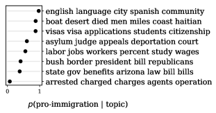
Figure 2: Topics inferred by a joint model of words and tone, and the corresponding probability of pro-immigration tone for each topic. A topic is represented by the top words sorted by word probability throughout the paper.

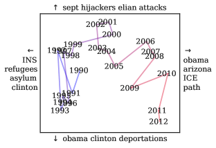
Figure 3: Learned embeddings of year-of-publication (treated as a covariate) from combined model of news articles about immigration.

5 Additional Related Work

The literature on topic models is vast; in addition to papers cited throughout, other efforts to incorporate metadata into topic models include Dirichlet-multinomial regression (DMR; Mimno and McCallum, 2008), Labeled LDA Ramage et al. (2009), and MedLDA Zhu et al. (2009). A recent paper also extended DMR by using deep neural networks to embed metadata into a richer document prior Benton and Dredze (2018).

A separate line of work has pursued parameterizing unsupervised models of documents using neural networks Hinton and Salakhutdinov (2009); Larochelle and Lauly (2012), including non-Bayesian approaches Cao et al. (2015). More recently, Lau et al. (2017) proposed a neural language model that incorporated topics, and He et al. (2017) developed a scalable alternative to the correlated topic model by simultaneously learning topic embeddings.

Others have attempted to extend the reparameterization trick to the Dirichlet and Gamma distributions, either through transformations (Kucukelbir et al., 2016) or a generalization of reparameterization (Ruiz et al., 2016). Black-box and VAE-style inference have been implemented in at least two general purpose tools designed to allow rapid exploration and evaluation of models (Kucukelbir et al., 2015; Tran et al., 2016).

6 Conclusion

We have presented a neural framework for generalized topic models to enable flexible incorporation of metadata with a variety of options. We take advantage of stochastic variational inference to develop a general algorithm for our framework such that variations do not require any model-specific algorithm derivations. Our model demonstrates the tradeoff between perplexity, coherence, and sparsity, and outperforms SLDA in predicting document labels. Furthermore, the flexibility of our model enables intriguing exploration of a text corpus on US immigration. We believe that our model and code will facilitate rapid exploration of document collections with metadata.

Supplementary Material

A Deriving the ELBO

The derivation of the ELBO for our model is given below, dropping explicit reference to $\bm{\Phi}$ and $\alpha$ for simplicity. For document $i$,

$$\log~{}p(\bm{w}_{i},\bm{y}_{i}\mid\bm{c}_{i})=\log\int_{\bm{r}_{i}}p(\bm{w}_{i},\bm{y}_{i},\bm{r}_{i}\mid\bm{c}_{i})d\bm{r}_{i}$$ (11)

$$=\log\int_{\bm{r}_{i}}p(\bm{w}_{i},\bm{y}_{i},\bm{r}_{i}\mid,\bm{c}_{i})\frac{q(\bm{r}_{i}\mid\bm{w}_{i},\bm{c}_{i},\bm{y}_{i})}{q(\bm{r}_{i}\mid\bm{w}_{i},\bm{c}_{i},\bm{y}_{i})}d\bm{r}_{i}$$ (12)

$$=\log\left(\mathbb{E}_{q(\bm{r}_{i}\mid\bm{w}_{i},\bm{c}_{i},\bm{y}_{i})}\left[\frac{p(\bm{w}_{i},\bm{y}_{i},\bm{r}_{i}\mid\bm{c}_{i})}{q(\bm{r}_{i}\mid\bm{w}_{i},\bm{c}_{i},\bm{y}_{i})}\right]\right)$$ (13)

$$\begin{aligned} \geq\mathbb{E}_{q(\bm{r}_{i}\mid\bm{w}_{i},\bm{c}_{i},\bm{y}_{i})}\left[\log p(\bm{w}_{i},\bm{y}_{i},\bm{r}_{i}\mid\bm{c}_{i})\right]\\ -\mathbb{E}_{q(\bm{r}_{i}\mid\bm{w}_{i},\bm{c}_{i},\bm{y}_{i})}\left[\log q(\bm{r}_{i}\mid\bm{w}_{i},\bm{c}_{i},\bm{y}_{i})\right]\end{aligned}$$ (14)

$$\begin{aligned} =\mathbb{E}_{q(\bm{r}_{i}\mid\bm{w}_{i},\bm{c}_{i},\bm{y}_{i})}&\left[\log p(\bm{w}_{i},\bm{y}_{i}\mid\bm{r}_{i},\bm{c}_{i})\right]\\ +\mathbb{E}_{q(\bm{r}_{i}\mid\bm{w}_{i},\bm{c}_{i},\bm{y}_{i})}&\left[\log p(\bm{r}_{i})\right]\\ -\mathbb{E}_{q(\bm{r}_{i}\mid\bm{w}_{i},\bm{c}_{i},\bm{y}_{i})}&\left[\log q(\bm{r}_{i}\mid\bm{w}_{i},\bm{c}_{i},\bm{y}_{i})\right]\end{aligned}$$ (15)

$$\begin{aligned} =\mathbb{E}_{q(\bm{r}_{i}\mid\bm{w}_{i},\bm{c}_{i},\bm{y}_{i})}&\left[\sum_{j=1}^{N_{i}}\log p(w_{ij}\mid\bm{r}_{i},\bm{c}_{i})\right]\\ +\mathbb{E}_{q(\bm{r}_{i}\mid\bm{w}_{i},\bm{c}_{i},\bm{y}_{i})}&\left[\log p(\bm{y}_{i}\mid\bm{r}_{i},\bm{c}_{i})\right]\\ -\textrm{D}_{\textrm{KL}}&\left[q(\bm{r}_{i}\mid\bm{w}_{i},\bm{c}_{i},\bm{y}_{i})~{}||~{}p(\bm{r}_{i})\right]\end{aligned}$$ (16)

B Model details

The KL divergence term in the variational bound can be computed as

$$\textrm{D}_{\textrm{KL}}[q_{\bm{\Phi}}(\bm{r}_{i}\mid\bm{w}_{i},\bm{c}_{i},\bm{y}_{i})\|p(\bm{r}_{i})]=\frac{1}{2}\left(\textrm{tr}(\bm{\Sigma}_{0}^{-1}\bm{\Sigma}_{i})+(\bm{\mu}_{i}-\bm{\mu}_{0})^{\top}\bm{\Sigma}_{0}^{-1}(\bm{\mu}_{i}-\bm{\mu}_{0})-K+\log\frac{|\bm{\Sigma}_{0}|}{|\bm{\Sigma}_{i}|}\right)$$ (17)

where $\bm{\Sigma}_{i}=\textrm{diag}(\bm{\sigma}_{i}^{2}(\bm{w}_{i},\bm{c}_{i},\bm{y}_{i}))$, and $\bm{\Sigma}_{0}=\textrm{diag}(\bm{\sigma}_{0}^{2}(\alpha))$.

C Practicalities and Implementation

As observed in past work, inference using a VAE can suffer from component collapse, which translates into excessive redundancy in topics (i.e., many topics containing the same set of words). To mitigate this problem, we borrow the approach used by Srivastava and Sutton (2017), and make use of the Adam optimizer with a high momentum, combined with batchnorm layers to avoid divergence. Specifically, we add batchnorm layers following the computation of $\bm{\mu}$, $\log\bm{\sigma}^{2}$, and $\bm{\eta}$.

This effectively solves the problem of mode collapse, but the batchnorm layer on $\bm{\eta}$ introduces an additional problem, not previously reported. At test time, the batchnorm layer will shift the input based on the learned population mean of the training data; this effectively encodes information about the distribution of words in this model that is not captured by the topic weights and background distribution. As such, although reconstruction error will be low, the document representation $\bm{\theta}$, will not necessarily be a useful representation of the topical content of each document. In order to alleviate this problem, we reconstruct $\bm{\eta}$ as a convex combination of two copies of the output of the generator network, one passed through a batchnorm layer, and one not. During training, we then gradually anneal the model from relying entirely on the component passed through the batchnorm layer, to relying entirely on the one that is not. This ensures that the the final weights and document representations will be properly interpretable.

Note that although ProdLDA Srivastava and Sutton (2017) does not explicitly include a background term, it is possible that the batchnorm layer applied to $\bm{\eta}$ has a similar effect, albeit one that is not as easily interpretable. This annealing process avoids that ambiguity.

D Data

All datasets were preprocessed by tokenizing, converting to lower case, removing punctuation, and dropping all tokens that included numbers, all tokens less than 3 characters, and all words on the stopword list from the snowball sampler. The vocabulary was then formed by keeping the words that occurred in the most documents (including train and test), up to the desired size (2000 for 20 newsgroups, 5000 for the others). Note that these small preprocessing decisions can make a large difference to perplexity. We therefore include our preprocessing scripts as part of our implementation so as to facilitate easy future comparison.

For the UIUC Yahoo answers dataset, we downloaded the documents from the project webpage. However, the file that is available does not completely match the description on the website. We dropped Cars and Transportation and Social Science which had less than the expected number of documents, and merged Arts and Arts and Humanities, which appeared to be the same category, producing 15 categories, each with 10,000 documents.

E Experimental Details

For all experiments we use a model with 300-dimensional embeddings of words, and we take $f_{e}$ to be only the element-wise softplus nonlinearity (followed by the linear transformations for $\bm{\mu}$ and $\log\bm{\sigma}^{2}$). Similarly, $f_{y}$ is a linear transformation of $\bm{\theta}$, followed by a softplus layer, followed by a linear transformation to the size of the output (the number of classes). During training, we set $S$ (the number of samples of $\bm{\epsilon}$) to be 1; for estimating the ELBO at on test documents, we set $S=20$.

For the unsupervised results, we use the same set up as Srivastava and Sutton (2017): Adam optimizer with $\beta_{1}=0.99$, learning rate $=0.002$, batch size of $200$, and training for $200$ epochs. The setup was the same for all datasets, except we only trained for $150$ epochs on Yahoo answers because it is much larger. For LDA, we updated the hyperparameters every 10 epochs.

For the external evaluation of NPMI, we use the co-occurrence statistics from all New York Times articles in the English Gigaword published from the start of 2000 to the end of 2009, processed in the same way as our data.

For the text classification experiments, we use the scikit-learn implementation of logistic regression. We give it access to the same input data as our model (using the same vocabulary), and tune the strength of $l_{2}$ regularization using cross-validation. For our model, we only tune the number of epochs, evaluating on development data. Our models for this task did not use regularization or word vectors.

F Additional Experimental Results

In this section we include additional experimental results in the unsupervised setting.

Table 4 shows results on the 20 newsgroups dataset, using 20 topics with a 2,000-word vocabulary. Note that these results are not necessarily directly comparable to previously published results, as preprocessing decisions can have a large impact on perplexity. These results show a similar pattern to those on the IMDB data provided in the main paper, except that word vectors do not improve internal coherence on this dataset, perhaps because of the presence of relatively more names and specialized terminology. Also, although the NVDM still has worse perplexity than LDA, the effects are not as dramatic as reported in Srivastava and Sutton (2017). Regularization is also more beneficial for this data, with both SAGE and our regularized model obtaining better coherence than LDA. The topics from scholar for this dataset are also shown in Table 6.

	Ppl.	NPMI	NPMI	Sparsity
Model	$\downarrow$	(int.) $\uparrow$	(ext.) $\uparrow$	$\uparrow$
LDA	810	0.20	0.11	0
SAGE	867	0.27	0.15	0.71
NVDM	1067	0.18	0.11	0
scholar - b.g.	928	0.17	0.09	0
scholar	921	0.35	0.16	0
scholar + w.v.	955	0.29	0.17	0
scholar + reg.	1053	0.25	0.13	0.43

Table 4: Performance of various models on the 20 newsgroups dataset with 20 topics and a 2,000-word vocabulary.

Table 5 shows the equivalent results for the Yahoo answers dataset, using 250 topics, and a 5,000-word vocabulary. These results closely match those for the IMDB dataset, with our model having higher perplexity but also higher internal coherence than LDA. As with IMDB, the use of word vectors improves coherence, both internally and externally, but again at the cost of worse perplexity. Surprisingly, our model without a background term actually has the best external coherence on this dataset, but as described in the main paper, these tend to give high weight primarily to common words, and are more repetitive as a result.

	Ppl.	NPMI	NPMI	Sparsity
Model	$\downarrow$	(int.) $\uparrow$	(ext.) $\uparrow$	$\uparrow$
LDA	1035	0.29	0.15	0
NVDM	4588	0.20	0.09	0
scholar - b.g.	1589	0.27	0.16	0
scholar	1596	0.33	0.13	0
scholar + w.v.	1780	0.37	0.15	0
scholar + reg.	1840	0.34	0.13	0.44

Table 5: Performance of various models on the Yahoo answers dataset with 250 topics and a 5,000-word vocabulary. SAGE did not finish in 72 hours so we omit it from this table.

NPMI	Topic
0.77	turks armenian armenia turkish roads escape soviet muslim mountain soul
0.52	escrow clipper encryption wiretap crypto keys secure chip nsa key
0.49	jesus christ sin bible heaven christians church faith god doctrine
0.43	fbi waco batf clinton children koresh compound atf went fire
0.41	players teams player team season baseball game fans roger league
0.39	guns gun weapons criminals criminal shooting police armed crime defend
0.37	playoff rangers detroit cup wings playoffs montreal toronto minnesota games
0.36	ftp images directory library available format archive graphics package macintosh
0.33	user server faq archive users ftp unix applications mailing directory
0.32	bike car cars riding ride engine rear bmw driving miles
0.32	study percent sexual medicine gay studies april percentage treatment published
0.32	israeli israel arab peace rights policy islamic civil adam citizens
0.30	morality atheist moral belief existence christianity truth exist god objective
0.28	space henry spencer international earth nasa orbit shuttle development vehicle
0.27	bus motherboard mhz ram controller port drive card apple mac
0.25	windows screen files button size program error mouse colors microsoft
0.24	sale shipping offer brand condition sell printer monitor items asking
0.21	driver drivers card video max advance vga thanks windows appreciated
0.19	cleveland advance thanks reserve ohio looking nntp western host usa
0.04	banks gordon univ keith soon pittsburgh michael computer article ryan

Table 6: Topics from the unsupervised scholar on the 20 newsgroups dataset, and the corresponding internal coherence values.

References

- Balasubramanyan et al. (2012) Ramnath Balasubramanyan, William W. Cohen, Doug Pierce, and David P. Redlawsk. 2012. Modeling polarizing topics: When do different political communities respond differently to the same news? In Proceedings of ICWSM.
- Benton and Dredze (2018) Adrian Benton and Mark Dredze. 2018. Deep Dirichlet multinomial regression. In Proceedings of NAACL.
- Blei et al. (2010) David M. Blei, Thomas L. Griffiths, and Michael I. Jordan. 2010. The nested Chinese restaurant process and Bayesian nonparametric inference of topic hierarchies. JACM, 57(2).
- Blei and Lafferty (2006) David M. Blei and John D. Lafferty. 2006. Dynamic topic models. In Proceedings of ICML.
- Blei et al. (2003) David M. Blei, Andrew Y. Ng, and Michael I. Jordan. 2003. Latent Dirichlet allocation. JMLR, 3:993–1022.
- Boyd-Graber et al. (2017) Jordan Boyd-Graber, Yuening Hu, and David Mimno. 2017. Applications of topic models. Foundations and Trends in Information Retrieval, 11(2-3):143–296.
- Cao et al. (2015) Ziqiang Cao, Sujian Li, Yang Liu, Wenjie Li, and Heng Ji. 2015. A novel neural topic model and its supervised extension. In Proceedings of AAAI.
- Card et al. (2015) Dallas Card, Amber E. Boydstun, Justin H. Gross, Philip Resnik, and Noah A. Smith. 2015. The media frames corpus: Annotations of frames across issues. In Proceedings of ACL.
- Cemgil (2009) Ali Taylan Cemgil. 2009. Bayesian inference for nonnegative matrix factorisation models. Computational Intelligence and Neuroscience, pages 4:1–4:17.
- Chang et al. (2009) Jonathan Chang, Sean Gerrish, Chong Wang, Jordan L Boyd-graber, and David M Blei. 2009. Reading tea leaves: How humans interpret topic models. In Proceedings of NIPS.
- Chang et al. (2008) Ming-Wei Chang, Lev-Arie Ratinov, Dan Roth, and Vivek Srikumar. 2008. Importance of semantic representation: Dataless classification. In Proceedings of AAAI.
- Das et al. (2015) Rajarshi Das, Manzil Zaheer, and Chris Dyer. 2015. Gaussian LDA for topic models with word embeddings. In Proceedings of ACL.
- Eisenstein et al. (2011) Jacob Eisenstein, Amr Ahmed, and Eric P. Xing. 2011. Sparse additive generative models of text. In Proceedings of ICML.
- Graff and Cieri (2003) David Graff and C Cieri. 2003. English gigaword corpus. Linguistic Data Consortium.
- He et al. (2017) Junxian He, Zhiting Hu, Taylor Berg-Kirkpatrick, Ying Huang, and Eric P. Xing. 2017. Efficient correlated topic modeling with topic embedding. In Proceedings of KDD.
- Hennig et al. (2012) Philipp Hennig, David Stern, Ralf Herbrich, and Thore Graepel. 2012. Kernel topic models. In Proceedings of AISTATS.
- Hinton and Salakhutdinov (2009) Geoffrey E Hinton and Ruslan R Salakhutdinov. 2009. Replicated softmax: An undirected topic model. In Proceedings of NIPS.
- Kingma and Welling (2014) Diederik P Kingma and Max Welling. 2014. Auto-encoding variational bayes. In Proceedings of ICLR.
- Kucukelbir et al. (2015) Alp Kucukelbir, Rajesh Ranganath, Andrew Gelman, and David Blei. 2015. Automatic variational inference in stan. In Proceedings of NIPS.
- Kucukelbir et al. (2016) Alp Kucukelbir, Dustin Tran, Rajesh Ranganath, Andrew Gelman, and David M. Blei. 2016. Automatic differentiation variational inference. ArXiv:1603.00788.
- Lafferty and Blei (2006) John D. Lafferty and David M. Blei. 2006. Correlated topic models. In Proceedings of NIPS.
- Larochelle and Lauly (2012) Hugo Larochelle and Stanislas Lauly. 2012. A neural autoregressive topic model. In Proceedings of NIPS.
- Lau et al. (2017) Jey Han Lau, Timothy Baldwin, and Trevor Cohn. 2017. Topically driven neural language model. In Proceedings of ACL.
- Maas et al. (2011) Andrew L. Maas, Raymond E. Daly, Peter T. Pham, Dan Huang, Andrew Y. Ng, and Christopher Potts. 2011. Learning word vectors for sentiment analysis. In Proceedings of ACL.
- McAuliffe and Blei (2008) Jon D. McAuliffe and David M. Blei. 2008. Supervised topic models. In Proceedings of NIPS.
- Miao et al. (2016) Yishu Miao, Lei Yu, and Phil Blunsom. 2016. Neural variational inference for text processing. In Proceedings of ICML.
- Mimno and McCallum (2008) David Mimno and Andrew McCallum. 2008. Topic models conditioned on arbitrary features with Dirichlet-multinomial regression. In Proceedings of UAI.
- Newman et al. (2010) David Newman, Jey Han Lau, Karl Grieser, and Timothy Baldwin. 2010. Automatic evaluation of topic coherence. In Proceedings of ACL.
- Nguyen et al. (2015a) Dat Quoc Nguyen, Richard Billingsley, Lan Du, and Mark Johnson. 2015a. Improving topic models with latent feature word representations. In Proceedings of ACL.
- Nguyen et al. (2015b) Viet-An Nguyen, Jordan Boyd-Graber, Philip Resnik, and Kristina Miler. 2015b. Tea party in the house: A hierarchical ideal point topic model and its application to Republican legislators in the 112th congress. In Proceedings of ACL.
- Nguyen et al. (2013) Viet-An Nguyen, Jordan L. Boyd-Graber, and Philip Resnik. 2013. Lexical and hierarchical topic regression. In Proceedings of NIPS.
- Paisley et al. (2014) John William Paisley, David M. Blei, and Michael I. Jordan. 2014. Bayesian nonnegative matrix factorization with stochastic variational inference. In Handbook of Mixed Membership Models and Their Applications, pages 205–224.
- Ramage et al. (2009) Daniel Ramage, David Hall, Ramesh Nallapati, and Christopher D. Manning. 2009. Labeled LDA: A supervised topic model for credit attribution in multi-labeled corpora. In Proceedings of EMNLP.
- Rezende et al. (2014) Danilo J. Rezende, Shakir Mohamed, and Daan Wierstra. 2014. Stochastic backpropagation and approximate inference in deep generative models. In Proceedings of ICML.
- Roberts et al. (2014) Molly Roberts, Brandon Stewart, Dustin Tingley, Christopher Lucas, Jetson Leder-Luis, Shana Gadarian, Bethany Albertson, and David Rand. 2014. Structural topic models for open ended survey responses. American Journal of Political Science, 58:1064–1082.
- Rosen-Zvi et al. (2004) Michal Rosen-Zvi, Thomas Griffiths, Mark Steyvers, and Padhraic Smyth. 2004. The author-topic model for authors and documents. In Proceedings of UAI.
- Ruiz et al. (2016) Francisco J R Ruiz, Michalis K Titsias, and David M Blei. 2016. The generalized reparameterization gradient. In Proceedings of NIPS.
- Srivastava and Sutton (2017) Akash Srivastava and Charles Sutton. 2017. Autoencoding variational inference for topic models. In Proceedings of ICLR.
- Tran et al. (2016) Dustin Tran, Alp Kucukelbir, Adji B. Dieng, Maja Rudolph, Dawen Liang, and David M. Blei. 2016. Edward: A library for probabilistic modeling, inference, and criticism. ArXiv:1610.09787.
- Wallach (2016) Hanna Wallach. 2016. Interpretability and measurement. EMNLP Workshop on Natural Language Processing and Computational Social Science.
- Wallach et al. (2009) Hanna Wallach, David M. Mimno, and Andrew McCallum. 2009. Rethinking LDA: Why priors matter. In Proceedings of NIPS.
- Yogatama et al. (2011) Dani Yogatama, Michael Heilman, Brendan O’Connor, Chris Dyer, Bryan R Routledge, and Noah A Smith. 2011. Predicting a scientific community’s response to an article. In Proceedings of EMNLP.
- Zhu et al. (2009) Jun Zhu, Amr Ahmed, and Eric P. Xing. 2009. MedLDA: Maximum margin supervised topic models for regression and classification. In Proceedings of ICML.