Vibronic Ground-state Degeneracies and the Berry Phase: A Continuous Symmetry Perspective

Abstract

We develop a geometric construction to prove the inevitability of the electronic ground-state (adiabatic) Berry phase for a class of Jahn-Teller models with maximal continuous symmetries and $N>2$ intersecting electronic states. Given that vibronic ground-state degeneracy in JT models may be seen as a consequence of the electronic Berry phase, and that any JT problem may be obtained from the subset we investigate in this letter by symmetry-breaking, our arguments reveal the fundamental origin of the vibronic ground-state degeneracy of JT models.

The Jahn-Teller (JT) theorem Jahn and Teller (1937); Jahn (1938) is a cornerstone of condensed matter and chemical physics; it enunciates that adiabatic electronically degenerate states of symmetric nonlinear molecules are unstable with respect to symmetry-breaking distortions of the molecular geometry (unless the degeneracy is protected by time-reversal symmetry). Given this statement, one might be tempted to loosely extrapolate that molecular quantum state degeneracies are generally unstable. This is, however, an incorrect conclusion: It is interesting that a large class of JT models exhibit robust vibronic ground-state degeneracies Longuet-Higgins et al. (1958); O’Brien (1969); Zwanziger and Grant (1987); Ham (1987, 1990); Cullerne and O’Brien (1994); De Los Rios et al. (1996); Chancey and O’Brien (1997); Bersuker (2006); Requist et al. (2016); Ryabinkin and Izmaylov (2013). Thus, there is a counterintuitive flavor to the JT theorem: vibronic degeneracies can be born at the expense of the breakdown of their electronic counterparts Bersuker (2006); Chancey and O’Brien (1997). These degeneracies leave distinctive signatures in the chemical dynamics of JT systems which are sometimes immune to degeneracy-breaking perturbations Ryabinkin and Izmaylov (2013); Joubert-Doriol and F. Izmaylov (2017). The goal of this letter is to explain the fundamental reason for the emergence of degenerate vibronic ground-states in JT models.

Vibronic ground-state degeneracy (VGSD) in JT models appears frequently when linear vibronic couplings dominate Bersuker (2006); Chancey and O’Brien (1997) (for a recent proposal of direct non-interferometric experimental verification of VGSD, see e.g.,Englman (2016, 2016)), although there are exceptions Moate et al. (1996); Bevilacqua et al. (2001); Bersuker (2001); Lijnen and Ceulemans (2005). More specifically, there exists a particular class of JT models for which VGSD is guaranteed to exist whenever the adiabatic approximation (Born-Oppenheimer Born and Oppenheimer (1927) with inclusion of Berry phase effects Mead and Truhlar (1979); Berry (1984)) is valid Bersuker (2006); Chancey and O’Brien (1997); Ribeiro and Yuen-Zhou (2017). These are the JT systems containing continuous symmetries and all possible couplings between JT active modes and a single electronically degenerate multiplet (at the reference geometry for a description of the JT effect, from now on denoted by JT center) Longuet-Higgins et al. (1958); O’Brien (1969); Judd (1974, 1982); Pooler and O’Brien (1977); Pooler (1978, 1980); Ribeiro and Yuen-Zhou (2017), the simplest and most famous example being the linear $E\otimes e$ model (we use the standard convention where the electronic irreducible representation (irrep) is given by a capital letter and the vibrational irrep is given by a lowercase) which displays an exotic SO(2) (circular) symmetry in its potential energy surface Longuet-Higgins et al. (1958); Bersuker (2006). The most complex spinless example is the SO(5)-invariant model of the icosahedral JT problem $H\otimes(g\oplus 2h)$, which contains all possible JT active modes associated with the electronic $H$ quintuplet Pooler (1980); Ceulemans, A. and Fowler, R. (1990); De Los Rios et al. (1996); Chancey and O’Brien (1997). On the other hand, the linearized $H\otimes h$ model has SO(3) symmetry Khlopin et al. (1978), but it does not include the couplings between $H$ and the remaining $g\oplus h$ active vibrations. In this letter we focus only on the former class of models, which we refer hereafter as JT systems with maximal continuous symmetries (MCSs) ($H\otimes h$ has SO(3) symmetry Khlopin et al. (1978), but inclusion of equally coupled $g\oplus h$ vibrations leads to a JT Hamiltonian invariant under the action of SO(5) Pooler (1980); the latter is the maximal symmetry group available for a JT model containing a single electronic $H$ multiplet Pooler (1980); De Los Rios et al. (1996)). Nevertheless, as we argue below, the results we obtain are expected to be meaningful also in the presence of moderate symmetry-breaking perturbations, as continuous symmetry is not a necessary condition for VGSD Bersuker (2006)).

We will discuss only JT models for which spin-orbit coupling can be neglected, so we may take the system to be spinless and the time-reversal operator $T$ to satisfy $T^{2}=1$. In all cases where it appears, VGSD in JT models can be associated to a twisting of the lowest-energy adiabatic electronic state as the molecular geometry traverses a loop on a vibrational configuration space submanifold enclosing the jT center. That is, a direct connection exists between the geometric phase Berry (1984); Mead (1992); Bohm et al. (2003) and the exotic degeneracy in the molecular ground-state of a large class of JT models Zwanziger and Grant (1987); Ham (1987); Ceulemans and Szopa (1991); Cullerne and O’Brien (1994); De Los Rios et al. (1996); Chancey and O’Brien (1997); Bersuker (2006); Requist et al. (2016); Ribeiro and Yuen-Zhou (2017); Bohm et al. (2003); Ham (1990).

In the limit where the ratio of the squared reduced (linear) vibronic constant to the harmonic restoring force at the JT center is large, the extrema of the electronic ground-state adiabatic potential energy surface (APES) are located sufficiently far from the JT center Bersuker (2006). The energy gap between the electronic ground-state and any other state in the considered multiplet is also generally large enough, and the adiabatic approximation holds. In this case, VGSD in JT models with MCSs arises from the following facts Bersuker (2006); Chancey and O’Brien (1997): (i) Continuous symmetry implies the space of minima of the ground-state APES is a continuous trough Pooler (1978); Judd (1984); Ceulemans (1987); Ribeiro and Yuen-Zhou (2017). (ii) If the choice is made that the electronic ground-state wavefunction is real for any nuclear geometry, then it can only change by $\pm 1$ when transported over a loop on the trough. (iii) Whenever this process leads to a change in sign of the electronic ground-state wavefunction, then, because the total vibronic wavefunction is single-valued, the corresponding nuclear wavefunction must satisfy compensating antiperiodic boundary conditions Longuet-Higgins et al. (1958); O’Brien (1969); Cullerne and O’Brien (1994); De Los Rios et al. (1996); Chancey and O’Brien (1997); this turns out to be the case for JT models with MCSs. (iv) Motion on the trough (pseudorotation) is equivalent to that of a free particle on a sphere with antipodal points identified by an equivalence relation O’Brien (1969); Ceulemans (1987); De Los Rios et al. (1996); Chancey and O’Brien (1997); Ribeiro and Yuen-Zhou (2017), and thus, the vibrational Schrodinger equation describing pseudorotation is the same as that for a point particle constrained to move on a sphere with appropriate boundary conditions. (v) The lowest energy wavefunction for a free particle on a spherical surface is symmetric under inversion; however, due to item (iii), it cannot be the ground-state vibrational wavefunction for JT models with MCSs. As a result, the molecular ground-state corresponds to the lowest-energy multiplet of a particle on a sphere with wavefunctions odd under inversion. (vi) This condition is satisfied by the vector irreducible representation of the orthogonal group O($N$) (the symmetry group of the sphere $S^{N-1}$). (viii) Finally, the vector irreps of O($N$) have more than one real dimension for all $N>1$ (the O(2) case is atypical, since the relevant representation to the corresponding JT model is spanned by the time-reversal partners $e^{\pm i\phi/2}$; this representation is only irreducible in the presence of time-reversal symmetry) Barut and Raczka (1986); this result implies VGSD, where the degeneracy is determined by the dimensionality of the vector irrep of O($N$). The facts above have been verified on a case-by-case basis for all JT models with continuous symmetriesO’Brien (1969); Judd (1984); Ham (1987); Zwanziger and Grant (1987); Auerbach (1994); Cullerne and O’Brien (1994); De Los Rios et al. (1996); Chancey and O’Brien (1997). This list of items traces the origin of the aforementioned counterintuitive feature of the JT problem: the electronic degeneracy, even though lifted, leaves its signature in the resulting vibrational eigenspectrum. By analogy to the Aharonov-Bohm effect Aharonov and Bohm (1959), as the nuclei circulate the JT center, they nonlocally recognize its existence and inherit a degeneracy themselves.

Despite the existence of a variety of works on the Berry phase in JT and related models Zwanziger and Grant (1987); Chancey and O’Brien (1997); Ham (1987); De Los Rios et al. (1996); Chancey and O’Brien (1988); Ceulemans and Szopa (1991); Apsel et al. (1992); Cullerne and O’Brien (1994); Auerbach (1994); Schön and Köppel (1995); Manini and Rios (1998); Bohm et al. (2003); Varandas and Xu (2004); Lijnen and Ceulemans (2005); Garcia-Fernandez et al. (2006); Bersuker (2006); Althorpe et al. (2008); Zygelman (2017); Abedi et al. (2012); Ryabinkin and Izmaylov (2013); Englman (2016); Requist et al. (2016), to the best of our knowledge, the following question has yet to be answered: given that in a set of $N$ intersecting real electronic states, such that some, but not all states change sign under a non-trivial loop on the nuclear configuration space, why does the electronic ground-state of JT models with MCSs (and in cases where this symmetry is only slightly broken) always has a nontrivial Berry phase (items (ii) and (iii) above)? For example, consider the SO(3)-invariant version of the cubic JT problem $T\otimes(e\oplus t_{2})$ O’Brien (1969). Its APES trough has a constant electronic spectrum with a degenerate branch including two excited electronic states, while the ground-state is non-degenerate. As first verified by O’Brien O’Brien (1969), the real ground-state electronic wavefunction of this model is double-valued. In other words, there exists an obstruction to the definition of a continuous global real basis for the electronic ground-state Chancey and O’Brien (1988); Ceulemans and Szopa (1991). This obstruction implies the electronic ground-state has a Berry phase, i.e., there exists loops on the vibrational configuration space, which if traversed adiabatically lead to a change in the sign of the electronic ground-state wavefunction Longuet-Higgins (1975); Bohm et al. (2003). The degenerate subspace orthogonal to the adiabatic ground-state is spanned by two basis vectors, only one of which admits a nontrivial Berry phase (see Eqs. 18 and 19). The more complex SO(4) and SO(5) icosahedral models display the same features Cullerne and O’Brien (1994); De Los Rios et al. (1996); Chancey and O’Brien (1997). Notably, $E\otimes e$ is a special case as both the electronic ground- and excited-state display a non-trivial geometric phase Bersuker (2006). Conversely, as mentioned above, for $N>2$ there is a priori no reason for the lowest energy electronic state to correspond to a non-trivial line bundle Varandas and Xu (2004); Varandas (2010). Thus, in this letter we aim attention at models with MCSs and $N>2$. While the electronic ground-state Berry phase has been verified on a case-by-case basis for all of these models before, the steps required to demonstrate the existence of the Berry phase are algebraically lengthy even for relatively small $N$Chancey and O’Brien (1997). Additionally, prior arguments do not indicate the common origin of the Berry phase in all of these systems. Because more realistic JT and other molecular systems with electronic degeneracies may be understood to arise from symmetry breaking of JT models with MCSs, an explanation for the inevitability of the electronic ground-state Berry phase of the latter is also a foundation for an understanding of the former.

It is the main objective of this letter to provide a simple answer to the question raised in the previous paragraph. We aim to explain the basic geometric reason for VGSD in JT systems with MCSs. Importantly, JT models with MCSs are minimal models for molecular conical intersections, so the generic features we find here are also relevant for a wide variety of problems in photochemical dynamics both in gas and condensed phases Atanasov et al. (2011); Domcke et al. (2011); Halász et al. (2011); Domcke and Yarkony (2012); Gatti (2014) (for a recent review on the effects of the molecular Berry phase on nonadiabatic dynamics near conical intersection, see Ref. Ryabinkin et al. (2017)).

The molecular Hamiltonian for a JT model with MCS can be written as:

$$H=\frac{\mathbf{P}^{2}}{2}+\frac{\omega^{2}\mathbf{Q}^{2}}{2}+H_{\text{JT}}(\mathbf{Q}),$$ (1)

where $\mathbf{Q}$ is the vector of nuclear displacements from the JT center $\mathbf{Q}=0$, $\mathbf{P}$ is the corresponding conjugate momentum, and $H_{\text{JT}}(\mathbf{Q})$ is the electronic JT Hamiltonian. The latter acts only on the family of $N-$dimensional electronic Hilbert spaces $\mathcal{H}_{el}(\mathbf{Q})$, and depends linearly on $\mathbf{Q}$. Thus, $H_{\text{JT}}(\mathbf{Q})$ may be written as

$$H_{\text{JT}}(\mathbf{Q})=F\sum_{k=1}^{M}Q_{k}V_{k},$$ (2)

where $F$ is the reduced vibronic coupling constant (from the Wigner-Eckart theorem), and $\{V_{k}\}$ are Clebsch-Gordan matrices depending on the choice of electronic diabatic basis vectors $\ket{\psi_{k}}$, $k\in\{1,2,...,N\}$ forming a representation of the corresponding continuous group Pooler (1978, 1980). A fundamental property of the JT models with MCSs is that they have a continuous set of electronic ground-state minima $\mathcal{O}\subset\mathbb{R}^{M}$, where $\nabla_{\mathbf{Q}}\left[E_{\text{JT}}(\mathbf{Q})+\omega^{2}\mathbf{Q}^{2}/2\right]=0$ Ceulemans (1987); Pooler (1978, 1980); Ribeiro and Yuen-Zhou (2017). In each case the electronic spectrum for any molecular geometry in the trough $\mathcal{O}$ is given by Longuet-Higgins et al. (1958); O’Brien (1969); Ceulemans and Fowler (1989); Chancey and O’Brien (1997); Ribeiro and Yuen-Zhou (2017)

$$\text{spec}[H_{\text{JT}}(\mathbf{Q})]=\{x(Q),x(Q),...,x(Q),-(N-1)x(Q)\},$$

$$x(Q)>0,\mathbf{Q}\in\mathcal{O},$$ (3)

where $Q$ is the Euclidean length of the JT displacement vector $\mathbf{Q}$ (all points of a given trough have the same value of $Q$), and $x(Q)$ is a real function of $Q$. For any $\mathbf{Q}\in\mathcal{O}$, the JT Hamiltonian with spectrum given by Eq. 3 may be rewritten as Ribeiro and Yuen-Zhou (2017)

$$H_{\text{JT}}(\mathbf{Q})=\sum_{i=1}^{M}Q_{i}V_{i}=QU[\mathbf{\theta}(\mathbf{Q})]V_{M}U^{-1}[\mathbf{\theta}(\mathbf{Q})],$$ (4)

where $QV_{M}$ is the diagonal matrix with entries determined by the electronic spectrum for $\mathbf{Q}\in\mathcal{O}$ (in the order specified by Eq. 3), $\theta(\mathbf{Q})=(\theta_{1}(\mathbf{Q}),...,\theta_{N-1}(\mathbf{Q}))$ are SO$(N)$ parameters specifying a molecular geometry at $\mathcal{O}$ (if $\theta(\mathbf{Q})$ is multivalued, then a continuous local choice of representative is assumed to have been made), and $U(\theta)$ (we will sometimes omit the dependence of $\theta$ on $\mathbf{Q}$ for notational simplicity) is the SO($N$) transformation of the electronic Hilbert space at $\mathbf{Q}$ defined by

$$Q[U(\theta)V_{M}U^{-1}(\theta)]=\sum_{i=1}^{M}\underbrace{(R^{-1}(\theta)\mathbf{Q}_{M}^{T})_{i}}_{=Q_{i}}V_{i},$$ (5)

where $R^{-1}(\theta)$ is the SO($N$)$\subset$SO($M$) vibrational configuration space rotation (pseudorotation) which maps $\mathbf{Q}_{M}=Q\mathbf{e}_{M}$ into $\mathbf{Q}=\sum_{i=1}^{M}Q_{i}\mathbf{e}_{i}$, where the $\mathbf{e}_{i}$ are the unit vectors of the vibrational configuration space. For the sake of simplicity we chose $F=1$. Thus, we see that $\mathbf{Q}_{M}$ defines a reference JT distorted molecular structure for which $H_{\text{JT}}(\mathbf{Q})$ is already diagonal in the diabatic basis $\{\ket{\psi_{k}}\}$. Note that $N\leq M$ for all JT models with MCSs Pooler (1978, 1980); Judd (1982); Ribeiro and Yuen-Zhou (2017). As an example of the above definitions, consider the case of $E\otimes e$. Since only two electronic states are retained in this model, it follows that $N=2$, and the diabatic basis may be written as $\{\ket{\psi_{1}},\ket{\psi_{2}}\}$. Let $\mathbf{\sigma}=(\sigma_{x},\sigma_{z})$ denote a matrix vector (each entry corresponds to a Pauli matrix), and $\mathbf{Q}=(Q_{x},Q_{z})=Q\text{sin}\theta\mathbf{e}_{x}+Q\text{cos}\theta\mathbf{e}_{z}$ [where $\theta=\text{tan}^{-1}(Q_{x}/Q_{z})$] be the JT displacement from the maximally symmetric structure at $\mathbf{Q}=0$. In this case, the electronic Hamiltonian can be written as

$$H_{\text{JT}}^{E\otimes e}(\mathbf{Q})=\mathbf{Q}\cdot\sigma^{T}=Q\text{sin}(\theta)\sigma_{x}+Q\text{cos}(\theta)\sigma_{z},$$ (6)

$$H_{\text{JT}}^{E\otimes e}(\mathbf{Q})=Qe^{-i\sigma_{y}\theta/2}\sigma_{z}e^{i\sigma_{y}\theta/2},$$ (7)

$$H_{\text{JT}}^{E\otimes e}(\mathbf{Q})=QU[\theta(\mathbf{Q})]\sigma_{z}U^{-1}[\theta(\mathbf{Q})],\leavevmode\nobreak\ \text{where}\leavevmode\nobreak\$$ (8)

$$U[\theta(\mathbf{Q})]=e^{-i\sigma_{y}\theta(\mathbf{Q})/2}.$$ (9)

In the notation of Eq. 4, it follows that for $E\otimes e$, $M=2$ and $V_{2}=\sigma_{z}$. Hence, for a given $Q$, the molecular structure with vanishing diabatic couplings is given by $\theta=0$. We obtain the relationship expressed by Eq. 5 by setting $\mathbf{e}_{2}=\mathbf{e}_{z}$ and $\mathbf{Q}_{2}=Q(0,1)$, such that

$$H_{\text{JT}}^{E\otimes e}(\mathbf{Q})=QU(\theta)V_{2}U^{-1}(\theta)=\sum_{i=1}^{2}\left[R^{-1}(\theta)\mathbf{Q}_{2}^{T}\right]_{i}\sigma_{i},$$ (10)

where we employed the relationship

$$R^{-1}(\theta)\mathbf{e}_{z}^{T}=\begin{pmatrix}\text{cos}\theta&\text{sin}\theta\\ -\text{sin}\theta&\text{cos}\theta\end{pmatrix}\cdot\mathbf{e}_{z}^{T}=\left(\text{sin}\theta,\text{cos}\theta\right).$$ (11)

Eqs. $3-5$ generalize the $E\otimes e$ construction and display the basic property of JT models with MCSs: a change of basis of the electronic Hilbert space preserving its real structure (e.g., an SO($N)$ transformation) leads to an electronic Hamiltonian matrix that can also be obtained by a rotation of the vibrational configuration space Pooler (1978, 1980); Judd (1982); Ribeiro and Yuen-Zhou (2017). However, note that only $N-1$ of the $N(N-1)/2$ degrees of freedom of SO($N$) are required to identify a point of the ground-state trough of JT models with MCSs. This is a consequence of the spectrum given by Eq. 1. In particular, the subgroup SO$(N-1)\subset$ SO$(N)$ that acts non-trivially only on the electronically degenerate subspace commutes with $H_{\text{JT}}(\mathbf{Q})$. Therefore, its corresponding action on the vibrational configuration space is trivial and gives rise to no additional molecular structures with the electronic spectrum given by Eq. 1.

Let the eigenstate of $H_{\text{JT}}(\mathbf{Q}_{M})$ with lowest eigenvalue be written as $\ket{\phi_{0}(\mathbf{Q}_{M})}=\ket{\psi_{N}}$, (from Eqs. 4 and 5, it follows that $U[\theta(\mathbf{Q}_{M})]=U(0)=R(0)=1$). For any $\mathbf{Q}\in\mathcal{O}$ related to $\mathbf{Q}_{M}$ by a pseudorotation, i.e., $\mathbf{Q}=R^{-1}(\theta)\mathbf{Q}_{M}$, a normalized electronic ground-state wavefunction of $H_{\text{JT}}(\mathbf{Q})$ is

$$\ket{\phi_{0}(\mathbf{Q})}=U(\theta)\ket{\phi_{0}(\mathbf{Q}_{M})}=U(\theta)\ket{\psi_{N}},$$

$$\ket{\phi_{0}(\mathbf{Q})}=\sum_{i=1}^{N}c_{0i}[\theta(\mathbf{Q})]\ket{\psi_{i}},c_{0i}\in\mathbb{R}.$$ (12)

The excited states span the hyperplane $\mathcal{S}_{0}^{\perp}(\mathbf{Q})$ of the electronic Hilbert space $\mathcal{H}_{el}(\mathbf{Q})$ at $\mathbf{Q}\in\mathcal{O}$ that is perpendicular to the line defined by the adiabatic electronic ground-state $\mathcal{L}_{0}(\mathbf{Q})=\text{span}\{\ket{\phi_{0}(\mathbf{Q})}\}$. Because the ground-state of $H_{\text{JT}}(\mathbf{Q})$ is gapped we may decompose $\mathcal{H}_{el}(\mathbf{Q})$ uniquely for any $\mathbf{Q}\in\mathcal{O}$ into the direct sum:

$$\mathcal{H}_{el}(\mathbf{Q})=\mathcal{L}_{0}(\mathbf{Q})\oplus\mathcal{S}_{0}^{\perp}(\mathbf{Q}).$$ (13)

In addition, since $T^{2}=1$, we take $\mathcal{H}_{el}(\mathbf{Q})$ to be a real vector space. Thus, a normalized basis for $\mathcal{L}_{0}(\mathbf{Q})$ is given by Eq. 12. The only permissible orthogonal basis transformations of $\mathcal{L}_{0}(\mathbf{Q})$ are given by multiplication by $O(1)=\pm 1$. Conversely, any choice of basis for $\mathcal{S}_{0}^{\perp}(\mathbf{Q})$ can be redefined by orthogonal transformations belonging to O$(N-1)$.

For every $\mathbf{Q}\in\mathcal{O}$ we can define a sphere $S^{N-1}(\mathbf{Q})$ immersed in $\mathbb{R}^{N}$. Then, because $\ket{\phi_{0}(\mathbf{Q})}=\sum_{i=1}^{N}c_{0i}[\mathbf{Q}]\ket{\psi_{i}}$ belongs to a line, we can represent it as the outwards normal vector of $S^{N-1}(\mathbf{Q})$ at the point with coordinates $c_{0}[\mathbf{Q}]=(c_{01}[\mathbf{Q}],...,c_{0N}[\mathbf{Q}])$. The hyperplane $\mathcal{S}_{0}^{\perp}(\mathbf{Q})$ can be mapped onto the tangent space of $S^{N-1}(\mathbf{Q})$ at the point $c_{0}[\mathbf{Q}]$, i.e., there exists a map $\mathcal{S}_{0}^{\perp}(\mathbf{Q})\mapsto T_{c_{0}[\mathbf{Q}]}S^{N-1}(\mathbf{Q})$. The mappings described above can be locally given by hyperspherical unit vectors (e.g., if $N=3$, then the tangent space of $c_{0}[\mathbf{Q}]\in S^{2}(\mathbf{Q})$ can be taken as the span of the polar and azimuthal vectors $\mathbf{e}_{\theta}(\mathbf{Q})$ and $\mathbf{e}_{\phi}(\mathbf{Q})$, while the normal vector field is $\mathbf{e}_{r}(\mathbf{Q})$).

Adiabatic transport of the ground-state $\ket{\phi_{0}(\mathbf{Q})}$ over the trough $\mathcal{O}$ is implemented by defining a curve $\text{$\gamma$:}\leavevmode\nobreak\ [0,1]\rightarrow\mathcal{O}$ along which $\ket{\phi_{0}(\mathbf{Q})}$ is parallel-transported according to the connection defined by Berry (1984); Ceulemans and Szopa (1991); Bohm et al. (2003),

$$\braket{\phi_{0}(\mathbf{Q})}{\mathrm{d}\phi_{0}(\mathbf{Q})}=0.$$ (14)

This condition is necessarily satisfied by any choice of real local section of $\mathcal{L}_{0}(\mathbf{Q})$ (recall there exists two (normalized) possibilities $\pm c_{0}[\mathbf{Q}]$ for the electronic ground-state at a given $\mathbf{Q}\in\mathcal{O}$; a local section is a continuous choice of either one of those for some open subset of $\mathcal{O}$).

Now consider an adiabatic loop starting at arbitrary $\mathbf{Q}_{0}\in\mathcal{O}$

$$\gamma_{L} [0,1]\rightarrow\mathcal{O},$$:

$$t\mapsto\gamma_{L}(t),\leavevmode\nobreak\ \gamma_{L}(0)=\gamma_{L}(1)=\mathbf{Q}_{0}.$$ (15)

As $t$ varies between 0 and 1, $\mathbf{Q}$ traverses the closed path $\gamma_{L}(t)\in\mathcal{O}$ and $\ket{\phi_{0}[\gamma_{L}(t)]}$ is parallel-transported according to the adiabatic connection (Eq. 14). Its associated normal vector traces a path on the space $\mathcal{B}$ defined by the disjoint union of the spheres $S^{N-1}(\mathbf{Q})$ attached to each $\mathbf{Q}\in\mathcal{O}$,

$$\mathcal{B}\equiv\bigsqcup_{\mathbf{Q}\in\mathcal{O}}S^{N-1}(\mathbf{Q}).$$ (16)

Intuitively, parallel transport ensures that given an initial vector $\ket{\phi_{0}(\mathbf{Q}_{0})}$ and a continuous path $\gamma_{L}$ in $\mathcal{O}$, there is a uniquely defined continuous curve $\ket{\phi_{0}[\gamma_{L}(t)]}$. If adiabatic transport along $\gamma_{L}(t)$ corresponds to an open path on $\mathcal{B}$, then it must take $c_{0}(\mathbf{Q}_{0})$ at $t=0$ into $-c_{0}(\mathbf{Q}_{0})$ at $t=1$. In this case, while the nuclei undergo a loop in the space of allowed JT distortions, the normal vector corresponding to the electronic ground-state is mapped into its antipode; thus, a Berry phase ensues. Continuous loops $\gamma_{L}(t)\in\mathcal{O}$ satisfying the preceding conditions always exist, as the electronic ground-state trough $\mathcal{O}$ is topologically equivalent to the real projective space $\mathbb{R}P^{N-1}$ Ceulemans (1987); De Los Rios et al. (1996); Ribeiro and Yuen-Zhou (2017) (for a detailed discussion of this point, see Secs.III.B.1 and III.B.2 of Ref. Ribeiro and Yuen-Zhou (2017)). $\mathbb{R}P^{N-1}$ has loops that are lifted to open paths connecting antipodal points of $S^{N-1}$ Ceulemans (1987); Ribeiro and Yuen-Zhou (2017); Nakahara (2003); Lee (2010). These features are crucial elements of our proof. The topological equivalence between $\mathcal{O}$ and $\mathbb{R}P^{N-1}$ can be simply restated as there being a continuous bijection between molecular geometries $\mathbf{Q}\in\mathcal{O}$ and real pure-state projection operators $|\eta\rangle\langle\eta|$ with $|\eta\rangle=\sum_{i=1}^{N}d_{i}|\psi_{i}\rangle,\leavevmode\nobreak\ d_{i}\in\mathbb{R}$.

More formally, the argument just given may be rephrased in the following way: $\mathcal{O}\cong\mathbb{R}P^{N-1}$ Ceulemans (1987); De Los Rios et al. (1996); Chancey and O’Brien (1997); Ribeiro and Yuen-Zhou (2017) implies the existence of a continuous bijective map (with continuous inverse)

$$\Phi \mathcal{O}\rightarrow\mathbb{R}P^{N-1},$$:

$$\mathbf{Q}\mapsto\ket{\phi_{0}(\mathbf{Q})}\bra{\phi_{0}(\mathbf{Q})}.$$ (17)

As a result, the equivalence classes of loops (containing all closed paths which can be deformed continuously into each other) of $\mathbb{R}P^{N-1}$ and the space of ground-state minima $\mathcal{O}$ are equal Nakahara (2003); Lee (2010). The case where $N=2$ corresponds to the thoroughly investigated SO(2)-invariant linear $E\otimes e$ system Longuet-Higgins et al. (1958); Zwanziger and Grant (1987); Ceulemans and Szopa (1991); Bersuker (2006), the only JT model with a spherical trough (as $\mathbb{R}P^{1}\cong S^{1}$, but $\mathbb{R}P^{N-1}\neq S^{N-1}$ when $N>2$ Nakahara (2003); Lee (2010)). From now on we assume $N>2$.

The non-trivial class $[\gamma_{L}(t)]$ of $\mathbb{R}P^{N-1}$ loops can be lifted via the adiabatic connection (and a choice of local section for the initial point on $S^{N-1}(\mathbf{Q})$, e.g., $c_{0}[\mathbf{Q}]$ representing $\ket{\phi_{0}(\mathbf{Q})}$) to a class of open paths on $\mathcal{B}$: let $(\mathbf{Q},p)$ with $p\in S^{N-1}(\mathbf{Q})$, denote local coordinates for the bundle $\mathcal{B}$ defined by Eq. 16. Then, the lift to $\mathcal{B}$ of a non-trivial loop $\gamma_{L}(t)\in[\gamma_{L}(t)]$ is defined by the curve $\text{$\tilde{\gamma}_{L}$:}\leavevmode\nobreak\ [0,1]\rightarrow\mathcal{B}$ connecting the points $(\mathbf{Q}_{0},\pm c_{0}[\mathbf{Q}_{0}])$ Nakahara (2003); Lee (2010), i.e.,

$$\tilde{\gamma}_{L}(t)=(\gamma_{L}(t),C[\gamma_{L}(t)]),\leavevmode\nobreak\ t\in[0,1],$$

$$C[\gamma_{L}(0)]=(c_{01}[\mathbf{Q}_{0}],...,c_{0N}[\mathbf{Q}_{0}])=\ket{\phi_{0}(\mathbf{Q}_{0})},$$

$$C[\gamma_{L}(1)]=-C[\gamma_{L}(0)]=-\ket{\phi_{0}(\mathbf{Q}_{0})},$$ (18)

where $C[\gamma_{L}(t)]$ is the vector obtained by parallel transport of $\ket{\phi_{0}(\mathbf{Q}_{0})}$ along $\gamma_{L}(t)$ with the adiabatic connection (Eq. 14). The geometric phase of the electronic ground-state for any loop $\gamma^{\prime}(t)\in\mathcal{O}$ with lift $\tilde{\gamma}^{\prime}(t)\in\mathcal{B}$ is given by Berry (1984); Ceulemans and Szopa (1991); Mead (1992)

$$\Gamma_{\gamma^{\prime}}^{0}=\braket{C[\gamma^{\prime}(0)]}{C[\gamma^{\prime}(1)]}.$$ (19)

Given that $\ket{\phi_{0}(\mathbf{Q})}$ is a normal vector of $S^{N-1}(\mathbf{Q})$, and a non-trivial loop $\gamma_{L}$ of $\mathbb{R}P^{N-1}$ is lifted into an open path on the family (bundle) of spheres attached to each $\mathbf{Q}\in\mathcal{O}$, it follows that $\gamma_{L}$ provides a mapping of the normal vector at $c_{0}[\mathbf{Q}]\in S^{N-1}(\mathbf{Q})$ into that at $-c_{0}[\mathbf{Q}]\in S^{N-1}(\mathbf{Q})$ which in turn implies $\Gamma_{\gamma_{L}}^{0}=-1$. Figure 1 illustrates this result (for visualization purposes the representative lift $\tilde{\gamma}_{L}(t)$ is drawn on a single sphere).

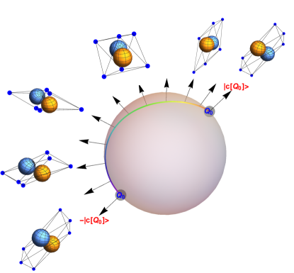
Figure 1: A visual representation of the lift $\tilde{\gamma}_{L}(t)$ (Eq. 18) of a non-trivial loop on the ground-state minimal energy trough $\mathcal{O}$ based at $\mathbf{Q}_{0}$, to the sphere bundle $\mathcal{B}$ for the SO(3)-invariant cubic model $T_{1}\otimes(e\oplus t_{2})$ O’Brien (1969) (see Eqs. 20 and 21). In this figure the path on the family of spheres parametrized by $\mathbf{Q}$ is represented on a single sphere for simplicity. The arrows correspond to a choice of local section for the normal vectors representing $\mathcal{L}_{0}(\mathbf{Q})$. The nontrivial $-1$ Berry phase of this model is indicated by the fact that the normal vector at $\mathbf{Q}_{0}$, $n(\mathbf{Q}_{0})$ is mapped into $-n(\mathbf{Q}_{0})$ under adiabatic transport over a loop on $\mathcal{O}$.

Our argument also implies that the number of linearly independent states which change sign under adiabatic transport on $\mathcal{O}$ is equal to the number of hyperspherical unit vectors of $S^{N-1}$ which have their sign changed under inversion of the sphere. For example, in the SO(3)-invariant model of $T_{1}\otimes(e\oplus t_{2})$ O’Brien (1969) the adiabatic ground-state is given by

$$\mathbf{e}_{r}\equiv\ket{\phi_{0}(\theta,\phi)}=\text{sin}\theta\text{cos}\phi\ket{\psi_{1}}+\text{sin}\theta\text{sin}\phi\ket{\psi_{2}}+\text{cos}\theta\ket{\psi_{3}},$$ (20)

where $\ket{\psi_{i}},i=1,2,3$, are electronic basis vectors spanning the $T_{1}$ irrep of the octahedral group, and for $\mathbf{Q}\in\mathcal{O}$ it follows that $\mathbf{Q}=\mathbf{Q}(\theta,\phi)=\mathbf{Q}(\pi-\theta,\phi+\pi)$ where $\theta\in[0,\pi],\phi\in[0,2\pi)$ O’Brien (1969). In fact, $\ket{\phi_{0}(\theta,\phi)}=-\ket{\phi_{0}(\pi-\theta,\phi+\pi)}$. The family of degenerate subspaces orthogonal to $\mathbf{e}_{r}(\theta,\phi)$ is generated by the basis vectors $\mathbf{e}_{\theta}(\theta,\phi)\equiv\ket{\phi_{1}(\theta,\phi)}$, and $\mathbf{e}_{\phi}(\theta,\phi)\equiv\ket{\phi_{2}(\theta,\phi)}$, where

$$\ket{\phi_{1}(\theta,\phi)}=\text{cos}\theta\text{cos}\phi\ket{\psi_{1}}+\text{cos}\theta\text{sin}\phi\ket{\psi_{2}}-\text{sin}\theta\ket{\psi_{3}},$$

$$\ket{\phi_{2}(\theta,\phi)}=-\text{sin}\phi\ket{\psi_{1}}+\text{cos}\phi\ket{\psi_{2}}.$$ (21)

Note that $\mathbf{e}_{\theta}[\mathbf{Q}]$ is fixed, but $\mathbf{e}_{\phi}[\mathbf{Q}]$ has its direction inverted when $(\theta,\phi)\mapsto(\pi-\theta,\pi+\phi)$. Similar verifications may be performed for the SO(4) and SO(5) icosahedral JT models Varandas and Xu (2004); Varandas (2010). In every case, only the normal vector corresponding to the ground-state and one of the spherical basis vectors of $\mathcal{S}_{0}^{\perp}(\mathbf{Q})$ acquire a non-trivial phase when $\mathbf{Q}$ traverses a loop on $\mathcal{O}$. This can be understood by considering the behavior of hyperspherical basis vectors under inversion of $S^{N-1}$. Previous work by Varandas and Xu Varandas and Xu (2004) provided the possible sign changes of the electronic adiabatic states of JT models (see also Ref.Varandas (2010)) by explicitly constructing the higher-dimensional counterparts of Eqs. 20 and 21, though their considerations did not uncover the fundamental reason the lowest-energy state of JT models with MCSs always admits a nontrivial Berry phase.

At first sight our construction may be perceived as severely restricted by the conditions that (a) the molecular Hamiltonian is totally symmetric under the action of a continuous group on the electronic and vibrational degrees of freedom and (b) the ground-state trough $\mathcal{O}$ has the electronic spectrum described by Eq. 1. However, higher-order vibronic perturbations which remove these constraints may only change the Berry phase if they induce degeneracies between the adiabatic ground-state $\ket{\phi_{0}(\mathbf{Q})}$ and any other electronic state in regions relevant to nuclear dynamics at low energies. This will happen e.g., if sufficiently strong quadratic vibronic couplings are introduced Zwanziger and Grant (1987); Koizumi and Bersuker (1999); Koizumi et al. (2000). Alternatively, any external perturbation (e.g., due to a static electric field) which couples the degenerate states will lift their degeneracy Bersuker (2006). In other words, while generic perturbations typically break MCSs and lead to a discrete set of ground-state minima (as opposed to a continuous trough) Zwanziger and Grant (1987); Koizumi and Bersuker (1999); Koizumi et al. (2000); Bersuker (2006) the Berry phase may still persist. Therefore, while the existence of a ground-state trough is significant to our proof, it is not a necessary condition for the existence of VGSD.

In summary, the reason that VGSD exists in spinless JT models with MCSs is that the adiabatic electronic ground-state corresponding to every geometry $\mathbf{Q}$ in the space $\mathcal{O}$ of JT APES minima can be canonically mapped to a normal vector of a sphere attached to each $\mathbf{Q}$, while its orthogonal subspace can be mapped onto the tangent space at the same point. Under adiabatic transport over a non-trivial loop on $\mathcal{O}$ the spherical normal vector corresponding to the electronic ground-state has its direction reversed, thereby giving a Berry phase, and requiring antiperiodic boundary conditions to be satisfied by the nuclear wavefunction, for the total vibronic ground-state to be single-valued. It is crucial for the existence of a Berry phase that the aforementioned non-trivial paths exist and are relevant for the dynamics of the physical system at low energies. These pre-requisites are ensured here by the topological equivalence between the nuclear trough $\mathcal{O}$ and the electronic projective space $\mathbb{R}P^{N-1}$ Ceulemans (1987); Ribeiro and Yuen-Zhou (2017), and by the fact that the Born-Oppenheimer potential energy is constant in $\mathcal{O}$. In other words, our construction relied on two key features of JT models with MCSs: (i) the topological equivalence between the JT trough $\mathcal{O}$ and the real projective Hilbert space, and (ii) the existence of a uniquely defined electronic ground-state line $\mathcal{L}_{0}(\mathbf{Q})$ and excited degenerate subspace $\mathcal{S}_{0}^{\perp}(\mathbf{Q})$ perpendicular to $\mathcal{L}_{0}(\mathbf{Q})$ at all $\mathbf{Q}\in\mathcal{O}$. Although these conditions are ideal, as explained, VGSD is protected as long as perturbations breaking the MCS of the studied models are not strong enough that intersections between the electronic ground-state and the remaining states emerge in low-energy regions of the ground-state APES. Therefore, we believe the presented construction provides the fundamental reason for the prevalence of VGSD in a large class of JT models. It would be interesting to understand whether these topological degeneracies can emerge in other contexts, such as optical or mechanical systems.

Acknowledgments.– Both authors acknowledge support from NSF CAREER award CHE:1654732 and generous UCSD startup funds.

References

- Jahn and Teller (1937) Jahn, H. A.; Teller, E. Stability of Polyatomic Molecules in Degenerate Electronic States. I. Orbital Degeneracy. Proc. R. Soc. London, Ser. A 1937, 161, 220–235.
- Jahn (1938) Jahn, H. A. Stability of Polyatomic Molecules in Degenerate Electronic States. II. Spin Degeneracy. Proc. R. Soc. London, Ser. A 1938, 164, 117–131.
- Longuet-Higgins et al. (1958) Longuet-Higgins, H. C.; Opik, U.; Pryce, M. H. L.; Sack, R. A. Studies of the Jahn-Teller Effect. II. The Dynamical Problem. Proc. R. Soc. London, Ser. A 1958, 244, 1–16.
- O’Brien (1969) O’Brien, M. C. M. Dynamic Jahn-Teller Effect in an Orbital Triplet State Coupled to Both and Vibrations. Phys. Rev. 1969, 187, 407–418.
- Zwanziger and Grant (1987) Zwanziger, J. W.; Grant, E. R. Topological Phase in Molecular Bound States: Application to the System. J. Chem. Phys. 1987, 87, 2954–2964.
- Ham (1987) Ham, F. S. Berry’s Geometrical Phase and the Sequence of States in the Jahn-Teller Effect. Phys. Rev. Lett. 1987, 58, 725–728.
- Ham (1990) Ham, F. S. The Role of Berry’s Phase in Ordering the Low-Energy States of a Jahn-Teller System in Strong Coupling. J. Phys.: Condens. Matter 1990, 2, 1163–1177.
- Cullerne and O’Brien (1994) Cullerne, J. P.; O’Brien, M. C. M. The Jahn-Teller Effect in Icosahedral Symmetry: Ground-State Topography and Phases. Journal of Physics: Condensed Matter 1994, 6, 9017–9041.
- De Los Rios et al. (1996) De Los Rios, P.; Manini, N.; Tosatti, E. Dynamical Jahn-Teller Effect and Berry Phase in Positively Charged Fullerenes: Basic Considerations. Phys. Rev. B 1996, 54, 7157–7167.
- Chancey and O’Brien (1997) Chancey, C.; O’Brien, M. The Jahn-Teller Effect in C60 and Other Icosahedral Complexes; Princeton University Press: Princeton, USA.; 1997.
- Bersuker (2006) Bersuker, I. The Jahn-Teller Effect; Cambridge University Press: Cambridge, U.K.; 2006.
- Requist et al. (2016) Requist, R.; Tandetzky, F.; Gross, E. K. U. Molecular Geometric Phase from the Exact Electron-Nuclear Factorization. Phys. Rev. A 2016, 93, 042108.
- Ryabinkin and Izmaylov (2013) Ryabinkin, I. G.; Izmaylov, A. F. Geometric Phase Effects in Dynamics Near Conical Intersections: Symmetry Breaking and Spatial Localization. Phys. Rev. Lett. 2013, 111, 220406.
- Joubert-Doriol and F. Izmaylov (2017) Joubert-Doriol, L.; F. Izmaylov, A. Molecular ”Topological Insulators”: A Case Study of Electron Transfer in the Bis(Methylene) Adamantyl Carbocation. Chemical Communications 2017, 53, 7365–7368.
- Englman (2016) Englman, R. Spectroscopic Detectability of the Molecular Aharonov-Bohm Effect. J. Chem. Phys. 2016, 144, 024103.
- Englman (2016) Englman, R. Non-Interferometric Determination of Berry Phases: Precession Reversal in Noiseless Systems. J. Chem. Phys. 2016, 145, 184105.
- Moate et al. (1996) Moate, C. P.; O’Brien, M. C. M.; Dunn, J. L.; Bates, C. A.; Liu, Y. M.; Polinger, V. Z. : A Jahn-Teller Coupling That Really Does Reduce the Degeneracy of the Ground State Physical Review Letters 1996, 77, 4362–4365.
- Bevilacqua et al. (2001) Bevilacqua, G.; Bersuker, I.; Martinelli, L. Vibronic Interactions: Jahn-Teller Effect in Crystals and Molecules; Springer, 2001; pp 229–233.
- Bersuker (2001) Bersuker, I. B. Vibronic Interactions: Jahn-Teller Effect in Crystals and Molecules; Springer, 2001; pp 73–82.
- Lijnen and Ceulemans (2005) Lijnen, E.; Ceulemans, A. Berry Phase and Entanglement in the Icosahedral H x (G+2h) Jahn-Teller System with Trigonal Minima. Phys. Rev. B 2005, 71, 014305.
- Born and Oppenheimer (1927) Born, M.; Oppenheimer, R. Zur Quantentheorie Der Molekeln. Ann. Phys (Berlin, Ger.) 1927, 389, 457–484.
- Mead and Truhlar (1979) Mead, C. A.; Truhlar, D. G. On the Determination of Born-Oppenheimer Nuclear Motion Wave Functions Including Complications Due to Conical Intersections and Identical Nuclei. J. Chem. Phys. 1979, 70, 2284–2296.
- Berry (1984) Berry, M. V. Quantal Phase Factors Accompanying Adiabatic Changes. Proc. R. Soc. London, Ser. A 1984, 392, 45–57.
- Ribeiro and Yuen-Zhou (2017) Ribeiro, R. F.; Yuen-Zhou, J. Continuous Vibronic Symmetries in Jahn-Teller Models: Local and Global Aspects. arXiv:1705.08104, 2017.
- Judd (1974) Judd, B. R. Lie Groups and the Jahn-Teller Effect. Can. J. Phys. 1974, 52, 999–1044.
- Judd (1982) Judd, B. R. The Dynamical Jahn-Teller Effect in Localized Systems. Yu E. Perlin and M. Wagner, Eds.; North-Holland: Amsterdam, 1982.
- Pooler and O’Brien (1977) Pooler, D. R.; O’Brien, M. C. M. The Jahn-Teller Effect in a Quartet: Equal Coupling to and Vibrations. J. Phys. C: Solid State Phys. 1977, 10, 3769–3792.
- Pooler (1978) Pooler, D. R. Continuous Group Invariances of Linear Jahn-Teller Systems. J. Phys. A: Math. Gen. 1978, 11, 1045–1056.
- Pooler (1980) Pooler, D. R. Continuous Group Invariances of Linear Jahn-Teller Systems. II. Extension and Application to Icosahedral Systems. J. Phys. C: Solid State Phys. 1980, 13, 1029–1042.
- Ceulemans, A. and Fowler, R. (1990) Ceulemans, A., Fowler, R. The Jahn-Teller Instability of Fivefold Degenerate States in Icosahedral Molecules. J. Chem. Phys. 1990, 93, 1221–1234.
- Khlopin et al. (1978) Khlopin, V. P.; Polinger, V. Z.; Bersuker, I. B. The Jahn-Teller Effect in Icosahedral Molecules and Complexes. Theor. Chim. Acta 1978, 48, 87–101.
- Mead (1992) Mead, C. A. The Geometric Phase in Molecular Systems. Rev. Mod. Phys. 1992, 64, 51–85.
- Bohm et al. (2003) Bohm, A.; Koizumi, H.; Niu, Q.; Zwanziger, J.; Mostafazadeh, A. The Geometric Phase in Quantum Systems; Springer: New York, USA; 2003.
- Ceulemans and Szopa (1991) Ceulemans, A.; Szopa, M. The Berry Phase for a Threefold Degenerate State. J. Phys. A: Math. Gen. 1991, 24, 4495-4509.
- Judd (1984) Judd, B. R. In Advances in Chemical Physics; Prigogine, I., Rice, S. A., Eds.; John Wiley & Sons, Inc., 1984; pp 247–309.
- Ceulemans (1987) Ceulemans, A. The Structure of Jahn-Teller Surfaces. J. Chem. Phys. 1987, 87, 5374–5385.
- Barut and Raczka (1986) Barut, A.; Raczka, R. Theory of Group Representations and Applications; World Scientific Publishing Co Inc: Singapore; 1986.
- Auerbach (1994) Auerbach, A. Vibrations and Berry Phases of Charged Buckminsterfullerene. Phys. Rev. Lett. 1994, 72, 2931–2934.
- Aharonov and Bohm (1959) Aharonov, Y.; Bohm, D. Significance of Electromagnetic Potentials in the Quantum Theory. Phys. Rev. 1959, 115, 485–491.
- Chancey and O’Brien (1988) Chancey, C. C.; O’Brien, M. C. M. Berry’s Geometric Quantum Phase and the Jahn-Teller Effect. J. Phys. A: Math. Gen. 1988, 21, 3347–3353.
- Apsel et al. (1992) Apsel, S. E.; Chancey, C. C.; O’Brien, M. C. M. Berry Phase and the and the Jahn-Teller System. Phys. Rev. B 1992, 45, 5251–5261.
- Schön and Köppel (1995) Schön, J.; Köppel, H. Geometric Phase Effects and Wave Packet Dynamics on Intersecting Potential Energy Surfaces. J. Chem. Phys. 1995, 103, 9292–9303.
- Manini and Rios (1998) Manini, N.; Rios, P. D. L. The rôle of the Berry Phase in Dynamical Jahn-Teller Systems. J. Phys.: Condens. Matter 1998, 10, 8485–8495.
- Varandas and Xu (2004) Varandas, A. J. C.; Xu, Z. R. Geometric Phase Effect at N-Fold Electronic Degeneracies in Jahn-Teller Systems. Int. J. Quantum Chem. 2004, 99, 385–392.
- Garcia-Fernandez et al. (2006) Garcia-Fernandez, P.; Bersuker, I. B.; Boggs, J. E. Lost Topological (Berry) Phase Factor in Electronic Structure Calculations. Example: The Ozone Molecule. Phys. Rev. Lett. 2006, 96, 163005.
- Althorpe et al. (2008) Althorpe, S. C.; Stecher, T.; Bouakline, F. Effect of the Geometric Phase on Nuclear Dynamics at a Conical Intersection: Extension of a Recent Topological Approach from One to Two Coupled Surfaces. J. Chem. Phys. 2008, 129, 214117.
- Zygelman (2017) Zygelman, B. The Molecular Aharonov-Bohm Effect Redux. J. Phys. B: At., Mol. Opt. Phys. 2017, 50, 025102.
- Abedi et al. (2012) Abedi, A.; Maitra, N. T.; Gross, E. K. U. Correlated Electron-Nuclear Dynamics: Exact Factorization of the Molecular Wavefunction. J. Chem. Phys. 2012, 137, 22A530.
- Longuet-Higgins (1975) Longuet-Higgins, H. C. The Intersection of Potential Energy Surfaces in Polyatomic Molecules. Proc. R. Soc. London, Ser. A 1975, 344, 147–156.
- Varandas (2010) Varandas, A. J. C. Geometrical Phase Effect in Jahn-Teller Systems: Twofold Electronic Degeneracies and Beyond. Chem. Phys. Lett. 2010, 487, 139–146.
- Atanasov et al. (2011) Atanasov, M.; Daul, C.; Tregenna-Piggott, P. L. Vibronic Interactions and the Jahn-Teller Effect: Theory and Applications; Springer Science & Business Media, 2011; Vol. 23.
- Domcke et al. (2011) Domcke, W.; Yarkony, D. R.; Köppel, H. Conical Intersections: Theory, Computation and Experiment Vol. 17; World Scientific: Singapore; 2011 .
- Halász et al. (2011) Halász, G. J.; Vibók, Á.; Šindelka, M.; Moiseyev, N.; Cederbaum, L. S. Conical Intersections Induced by Light: Berry Phase and Wavepacket Dynamics. J. Phys. B: At., Mol. Opt. Phys. 2011, 44, 175102.
- Domcke and Yarkony (2012) Domcke, W.; Yarkony, D. R. Role of Conical Intersections in Molecular Spectroscopy and Photoinduced Chemical Dynamics. Annu. Rev. Phys. Chem. 2012, 63, 325–352.
- Gatti (2014) Gatti, F. Molecular Quantum Dynamics: From Theory to Applications; Springer Science & Business Media, 2014.
- Ryabinkin et al. (2017) Ryabinkin, I. G.; Joubert-Doriol, L.; Izmaylov, A. F. Geometric Phase Effects in Nonadiabatic Dynamics near Conical Intersections. Acc. Chem. Res. 2017, 50, 1785–1793.
- Ceulemans and Fowler (1989) Ceulemans, A.; Fowler, P. W. SO(4) Symmetry and the Static Jahn-Teller Effect in Icosahedral Molecules. Phys. Rev. A 1989, 39, 481–493.
- Nakahara (2003) Nakahara, M. Geometry, Topology and Physics; CRC Press: Boca Raton, USA; 2003.
- Lee (2010) Lee, J. Introduction to Topological Manifolds; Springer Science & Business Media; 2010.
- Koizumi and Bersuker (1999) Koizumi, H.; Bersuker, I. B. Multiconical Intersections and Nondegenerate Ground State in Jahn-Teller Systems. Phys. Rev. Lett. 1999, 83, 3009–3012.
- Koizumi et al. (2000) Koizumi, H.; Bersuker, I. B.; Boggs, J. E.; Poilinger, V. Z. Multiple Lines of Conical Intersections and Nondegenerate Ground State in Jahn-Teller Systems. J. Chem. Phys. 2000, 112, 8470–8482.