Vacuum Topology and the Electroweak Phase Transition

Abstract

We investigate if the topology of pure gauge fields in the electroweak vacuum can play a role in classical dynamics at the electroweak phase transition. Our numerical analysis shows that magnetic fields are produced if the initial vacuum has non-trivial Chern-Simons number, and the fields are helical if the Chern-Simons number changes during the phase transition.

An explanation for the observed cosmic matter-antimatter asymmetry likely requires CP violating particle interactions at energies at or above the electroweak scale, at an epoch when the universe was out of thermal equilibrium Sakharov (1967). Models of matter-genesis, more specifically, baryogenesis or leptogenesis, also necessarily involve the violation of baryon plus lepton (B+L) number through anomalous quantum processes. Several studies have now shown that the anomalous violation of B+L at the time of electroweak symmetry breaking, when the Higgs ($\Phi$) acquires a non-vanishing vacuum expectation value (VEV), leads to the production of helical magnetic fields Cornwall (1997a); Vachaspati (2001a). The connection of matter-genesis and magneto-genesis offers a means to probe fundamental particle interactions by the observation of magnetic fields in the universe.

In hindsight it is not difficult to intuitively understand the production of helical magnetic fields when B+L is violated by anomalous processes. To change B+L, requires a change in the Chern-Simons number of the electroweak gauge fields and, post electroweak symmetry breaking, this requires passage through a “sphaleron” Manton (1983) that has the interpretation of a twisted magnetic monopole-antimonopole configuration Vachaspati and Field (1994); Hindmarsh and James (1994); Saurabh and Vachaspati (2017) The decay of the sphaleron corresponds to the annihilation of the monopole and antimonopole, with the release of helical magnetic fields Copi et al. (2008); Chu et al. (2011).

In the present paper, we address a related question – can the topology of the electroweak vacuum play a role in the dynamics of the electroweak phase transition? A hint that the answer is in the affirmative is suggested by the work of Jackiw and Pi Jackiw and Pi (2000), where they consider a pure vacuum SU(2) gauge field configuration that has non-vanishing Chern-Simons number. They then project the gauge field configuration onto a fixed isospin direction to simulate the effects of the Higgs field VEV, and then evolve and calculate the helicity in the electromagnetic (EM) field. Jackiw and Pi find a non-vanishing EM helicity and further provide the neat result that the EM helicity at late times is 1/2 of the helicity at early times.

As originally discussed in Ref. Jackiw and Pi (2000), the Jackiw-Pi result depends crucially on their model for projection of the gauge fields in isospin space. For example, note that the initial gauge configuration is pure gauge and has zero energy, while the final configuration with helical magnetic fields has non-zero energy. Clearly energy is introduced by the act of projecting the non-Abelian gauge fields to the Abelian component, and it is assumed that the projection somehow mimics electroweak symmetry breaking. In a more realistic setting, the projection will be achieved by the process by which the Higgs field acquires a VEV, and the precise projection in isospin space depends on the dynamics of the Higgs field as it interacts with the gauge (and other) fields.

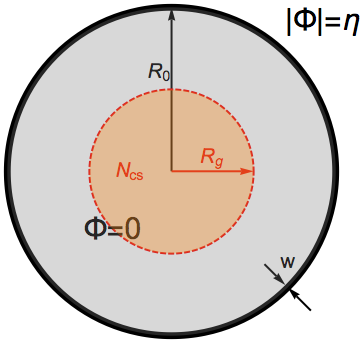
Figure 1: In a first-order electroweak phase transition, bubbles of true vacuum ($|\Phi|=\eta$) will grow and encapsulate regions of false vacuum ($\Phi=0$), within which gauge fields with localized non-trivial Chern-Simons number, $N_{\rm{CS}}$, may exist. With time, the bubbles of true vacuum will grow and complete the phase transition, forcing a projection of the gauge fields within the region of radius $R_{g}$ (shown as an orange disk) in the false vacuum onto the EM field. In studying this process, we will replace the complicated geometry of the symmetric phase by a spherical bubble of radius $R_{0}$ (thick solid circle) and thickness $w$.

In this paper we will resolve the effect of isospin projection on the gauge fields by studying the full dynamics of the Higgs field and the electroweak gauge fields. Our first analysis corresponds to dynamics during a first order electroweak phase transition. We will set up a pure gauge field configuration in a spherical region with vanishing Higgs VEV, surrounded by the true vacuum of the model where the Higgs has already acquired a VEV as shown in Fig. 1. As the spherical region with vanishing Higgs shrinks, the electroweak gauge fields will get projected on to the EM field and presumably some magnetic field will be generated. We calculate the energy and helicity of the magnetic field as a function of time, for several different values of the initial Chern-Simons number.

We also examine the case of a second order electroweak phase transition, as shown in Fig. 2. Here the Higgs VEV vanishes everywhere at the initial time but its time derivative is non-vanishing.

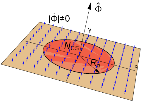
Figure 2: As a second-order electroweak phase transition proceeds, $\Phi=0$ everywhere but ${\dot{\Phi}}\neq 0$. (This is a simplification of the second order phase transition dynamics but one that is sufficient for our purposes.) The drawing shows a spatial slice over which $\Phi=0$ and with a localized region of pure gauge field with non-vanishing Chern-Simons number (red region). The blue arrows in the vertical direction illustrate the initial growth of the Higgs field VEV as in Eq. (9). As the VEV of $\Phi$ grows, pure gauge field configurations get projected into massless EM fields and massive gauge fields.

We start in Sec. I by describing the electroweak model and the initial conditions that we will use to study the evolution. We describe our numerical results in Sec. II both for a first-order transition (Sec. II.1) and for a second-order transition (Sec. II.2). We conclude in Sec. III. Further details of our numerical setup are provided in the appendices.

I Model details

The bosonic electroweak variables are the Higgs field $\Phi$, the SU(2) valued gauge fields $W^{a}_{\mu}$ and the U(1) hypercharge gauge field $B_{\mu}$, with Lagrangian

$$\mathcal{L}=|D_{\mu}\Phi|^{2}-\frac{1}{4}W^{a}_{\mu\nu}W^{a\mu\nu}-\frac{1}{4}B_{\mu\nu}B^{\mu\nu}-\lambda(|\Phi|^{2}-\eta^{2})^{2},$$ (1)

where

$$D_{\mu}=\partial_{\mu}-i\frac{g}{2}\sigma^{a}W^{a}_{\mu}-i\frac{g^{\prime}}{2}B_{\mu}$$ (2)

is the covariant derivative, $\sigma^{a}$ ($a=1,2,3$) the Pauli spin matrices, and $W^{a}_{\mu\nu}$, $B_{\mu\nu}$ are the field strengths. We describe the resulting equations of motion and our numerical techniques to solve them in Appendices A and B.

The initial conditions for the gauge fields are always pure gauge but can have non-trivial Chern-Simons number. As described in Jackiw and Pi (2000), these are

$$W_{\mu}\equiv\frac{\sigma^{a}}{2i}W^{a}_{\mu}=\frac{1}{g}U^{-1}\partial_{\mu}U\ ,\ \ B_{\mu}=0,$$ (3)

where,

$$U=\cos\frac{f(r)}{2}+i\bm{\sigma}\cdot\hat{\bm{\omega}}\sin\frac{f(r)}{2},$$ (4)

and the unit vector $\hat{\bm{\omega}}={\hat{x}}$ points in the radial direction and $r=|{\bm{x}}|$ is the radial spherical coordinate. The function $f(r)$ is chosen to be

$$f(r)=2\pi n\tanh(r/R_{g}),\ \ n=0,1,2,\ldots$$ (5)

Therefore the profile function $f(r)$ satisfies the boundary conditions $f(0)=0$ and $f(\infty)=2\pi n$. The time derivatives of all gauge fields are taken to vanish at the initial time $t=0$.

The Chern-Simons number is defined as

$$N_{\rm CS}(t) = \frac{N_{F}}{32\pi^{2}}\epsilon^{ijk}\int d^{3}x\biggl{[}-g^{\prime 2}B_{ij}B_{k}$$

$$+g^{2}\left(W^{a}_{ij}W^{a}_{k}-\frac{g}{3}\epsilon_{abc}W^{a}_{i}W^{b}_{j}W^{c}_{k}\right)\biggr{]},$$ (6)

where $N_{F}$ is the number of fermion families. In the rest of the paper, we will choose $N_{F}=1$. The initial gauge field configuration described in Eq. (3) has a Chern-Simons number

$$N_{\rm CS}=-n.$$ (7)

For the first-order phase transition set up shown in Fig. 1, the Higgs doublet is given by

$$\Phi(t=0,{\bm{r}}) = \frac{\eta}{2}\left[1+\tanh\left(\frac{r-R_{0}}{w}\right)\right]\begin{pmatrix}0\\ 1\end{pmatrix}$$

$$\dot{\Phi}(t=0,{\bm{r}}) = 0,$$ (8)

where $R_{0}>R_{g}$ is the initial size of the false vacuum region (the bubble), and $w\ll R_{0}$ is the width of the transition region from true to false vacuum, i.e. the bubble wall thickness.

One question that arises in the setup of the first order phase transition is that it should be possible to study the evolution after performing a large gauge transformation that makes the gauge fields trivial, $W_{i}=0$. If there is exactly zero overlap between the scalar and gauge profiles, such a gauge transformation will not affect the Higgs field (up to an overall sign). However, for profile functions that are analytic, such as the ones in Eqs. (5) and (8), there is always some overlap between the gauge fields and non-zero Higgs VEV. In this region $|D_{i}\Phi|\neq 0$ even for $i$ in the angular directions. The large gauge transformation that sets $W_{i}=0$ will also twist the Higgs. In fact, the electroweak model has two distinct and independent winding numbers: the gauge winding of Eq. (6) and the Higgs winding, $N_{w}$, e.g. as defined in Mou et al. (2017), and the difference of the two windings is invariant even under large gauge transformations. By gauging away the gauge winding, we will induce a corresponding Higgs winding. We have explicitly checked that the overlap between the Higgs and the gauge fields plays a crucial role in the evolution by also considering non-analytic profile functions, i.e. where the interior of the bubble has exactly $\Phi=0$ and the exterior of the gauge configuration has exactly $W_{i}=0$. Such non-analytic profiles are not expected to be relevant in a physical setting but they do show that no magnetic energy is produced if there is no overlap. The importance of the overlap will also be seen for analytic profiles when we demonstrate that the magnetic field energy grows with larger $R_{g}$.

Whereas for a second-order phase transition, the Higgs doublet is initially taken to be

$$\Phi(t=0,{\bm{r}}) = 0$$

$$\dot{\Phi}(t=0,{\bm{r}}) = \gamma\,\eta^{2}\begin{pmatrix}0\\ 1\end{pmatrix},$$ (9)

where $\gamma$ is a dimensionless parameter denoting the speed with which the uniform Higgs is rolling off the top of the potential. Our modelling of the second order phase transition is not completely accurate, since we hold the Higgs field at the origin until the potential has reached its zero temperature form. A more realistic treatment would take into account the temperature evolution of the potential over time scales set by the Hubble expansion, which is $\sim 10^{17}$ times slower than the electroweak time scale that determines the dynamical evolution rate of the fields in our simulations. We leave a more detailed investigation of these effects for future work. Nevertheless, we expect our treatment to fit more closely the actual cosmological phase transition than the sudden projection of the Chern-Simons vacuum onto massive and massless gauge field components that was used in Ref. Jackiw and Pi (2000).

Once the Higgs has left the symmetric phase, $\Phi=0$, we can track the EM magnetic field. The EM field potential is generally defined by

$$A_{\mu}=\sin\theta_{w}n^{a}W^{a}_{\mu}+\cos\theta_{w}B_{\mu},$$ (10)

and the EM field strength follows the definition in Vachaspati (1991a),

$$A_{\mu\nu} = \sin\theta_{w}n^{a}W^{a}_{\mu\nu}+\cos\theta_{w}B_{\mu\nu}$$ (11)

$$\hskip-31.2982pt-i\frac{2}{g|\Phi|^{2}}\sin\theta_{w}[(D_{\mu}\Phi)^{\dagger}(D_{\nu}\Phi)-(D_{\nu}\Phi)^{\dagger}(D_{\mu}\Phi)],$$

where, $\theta_{w}$ is the Weinberg angle, and $n^{a}$ is the unit vector in SU(2) isospace defined by the direction of the Higgs field

$$n^{a}=-\frac{\Phi^{\dagger}\sigma^{a}\Phi}{|\Phi|^{2}}.$$ (12)

These expressions are only defined when $|\Phi|\neq 0$. We shall alter them slightly so that the definition makes sense for all $\Phi$ and coincides with the usual definition in the symmetry broken phase. The expressions we use are

$$A_{\mu\hphantom{\nu}}=\sin\theta_{w}N^{a}W^{a}_{\mu}+\cos\theta_{w}B_{\mu}$$ (13)

$$A_{\mu\nu}=\sin\theta_{w}N^{a}W^{a}_{\mu\nu}+\cos\theta_{w}B_{\mu\nu}$$

$$\quad-i\frac{2}{g\eta^{2}}\sin\theta_{w}[(D_{\mu}\Phi)^{\dagger}(D_{\nu}\Phi)-(D_{\nu}\Phi)^{\dagger}(D_{\mu}\Phi)],$$ (14)

where,

$$N^{a}=-\frac{\Phi^{\dagger}\sigma^{a}\Phi}{\eta^{2}}.$$ (15)

We will also calculate the magnetic energy in the EM field

$$E_{\rm em}=\frac{1}{2}\int d^{3}x~{}{\bm{B}}^{2},$$ (16)

and the magnetic helicity

$$H_{\rm em}=\int d^{3}x~{}{\bm{A}}\cdot{\bm{B}}.$$ (17)

Our numerical scheme is based on a lattice implementation of the electroweak equations as described in Rajantie et al. (2001). The numerical details are listed in Appendix B. We adopt phenomenological values of all parameters: $g=0.65$, $\sin^{2}\theta_{w}=0.22$, $g^{\prime}=g\tan\theta_{w}$, $\eta=1$, $\lambda=0.129$. The Higgs mass is $m_{H}=2\eta\sqrt{\lambda}=125~{}\text{GeV}$, therefore $\eta=174~{}\text{GeV}$, which means one unit of energy in our simulation is equivalent to $174~{}\text{GeV}$. One unit of length is $1.13\times 10^{-16}~{}\text{cm}$, and one unit of time is $3.78\times 10^{-27}~{}\text{s}$.

We use absorbing boundary conditions (ABC) to minimize effects from lattice boundaries and to ensure that negligible contributions enter from outside the finite lattice box. It should be noted that the specific form of the ABC varies, depending on the initial conditions, as described in Appendix C. We run our simulation as long as the gauge fields are confined within the lattice box. Conservation of total energy and fulfillment of Gauss constraints are two non-trivial checks that we monitor in the simulation. The total energy is conserved within $1\%$, while the Gauss constraints given in Eq. (33) are satisfied to an even higher accuracy. Notice that both sets of initial conditions considered in this paper automatically satisfy the Gauss constraints, and thus should be preserved during the evolution in the bulk of the lattice; there may be small violations due to the boundary conditions on the lattice as discussed in Appendix B.

As a final check of our code, we have compared some results with a completely separate evolution code Vachaspati (2016) and obtained consistent results.

II Results

We will now describe the results of our simulations, first for the first order phase transition set up of Fig. 1, and then for the second order phase transition set up of Fig. 2.

II.1 First order phase transition

The Higgs field configuration at the initial time is given by Eq. (8). For our simulations we will set the false vacuum bubble radius to be $R_{0}=8.0$ and the bubble wall width to be $w=0.4$. At the center of the bubble we start with a pure gauge configuration as given in Eq. (3) with radius $R_{g}=6.0$. We denote the initial Chern-Simons number by $-n$. The case with $n=0$ has trivial evolution and no gauge fields are excited by the bubble collapse. The results for $n=1,2,3$ are non-trivial and are shown in Fig. 3 where we plot the evolution of the Chern-Simons number, the EM magnetic helicity defined in Eq. (17) and the EM magnetic energy defined in Eq. (16). We have tested the evolution with the definition of EM given in Eqs. (10) and (11) and find agreement at late times where these expressions are well-defined.

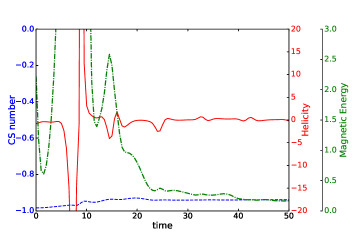
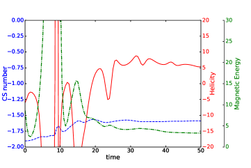
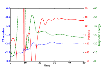
Figure 3: Plots of the Chern-Simons number (blue-dashed), magnetic helicity (red solid curve), and magnetic energy (green dot-dashed curve) for initial Chern-Simons number $n=1$ (top), $n=2$ (middle), and $n=3$ (bottom) in the first-order phase transition case. Note the different scale bars for the EM energy (in lattice units) shown on the right-hand side of the plot.

The total energies in our three runs with $n=1,2,3$ are about 964, 1083 and 1250, respectively and are well above the sphaleron barrier, which is $E_{\rm sph}\approx 9~{}{\rm TeV}$ Manton (1983); Klinkhamer and Manton (1984) or about 52 in lattice units. So there is ample energy in the simulations for the Chern-Simons number to change. Nevertheless, being above the sphaleron energy barrier is a necessary but not sufficient condition for the change in Chern-Simons number. Also note that the Chern-Simons number is an integer only for the vacuum; a non-vacuum configuration may have a non-integer value of the Chern-Simons number. Indeed, the plots in Fig. 3 show non-integer values of the Chern-Simons number as we always have some energy in the lattice.

In all our runs, there is some energy transferred from the false vacuum bubble to the gauge sector during evolution. This is seen in the plots of the EM energy, which is non-vanishing after the collapse of the bubble is complete. A non-vanishing positive helicity is obtained for the $n=2,3$ cases but not for the $n=1$ case for which the Chern-Simons number remains roughly constant. A rough fit to the data in Table I gives

$$|H_{\rm em}|\approx 56(\Delta N_{\rm CS})^{2}$$ (18)

where $\Delta N_{\rm CS}$ is the change in Chern-Simons number, and $n$ is the initial Chern-Simons number. Further, the sign of magnetic helicity is the same as the sign of the change in Chern-Simons number.

$n$	$\Delta N_{\rm CS}$	$H_{\rm em}$
1	$0.044$	$-0.20$
2	$0.31$	$5.4$
3	$0.77$	$33$

Table 1: $n$, $\Delta N_{\rm CS}$ and $H_{\rm em}$ for the first-order phase transition simulations. For $n=1$, $\Delta N_{\rm CS}$ and $H_{\rm em}$ are consistent with zero.

In Fig. 4 we show the electromagnetic energy as a function of time for several different values of the initial gauge radius $R_{g}$. The electromagnetic energy is larger for larger $R_{g}$. This is consistent with our expectations as discussed below Eq. (8) since larger $R_{g}$ provides greater overlap of the initial gauge fields and the imploding bubble.

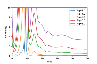
Figure 4: Plot of EM energy generated during a first-order phase transition for different $R_{g}$. The initial conditions are given by Eq. (3) and Eq. (8). Here, $R_{0}=8.0$, $w=0.4$, $n=2$.

II.2 Second order phase transition

The Higgs is now initially assumed to be in the symmetry unbroken phase everywhere but in the process of rolling down the potential toward the true vacuum (see Fig. 2 and Eq. (9)). In this case we need to specify the initial velocity of the Higgs field, the extent of the gauge field configuration, and the initial Chern-Simons number. We set the velocity parameter $\gamma=0.4$ and the radius of the gauge field configuration $R_{g}=6.0$. Three different initial Chern-Simons number are considered: $n=1,2,3$. As in the first-order phase transition case, the evolution for $n=0$ is trivial.

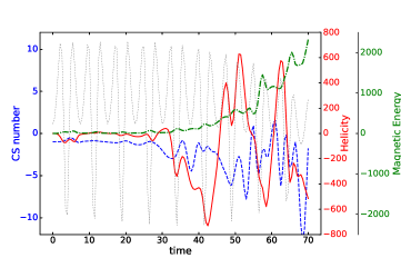
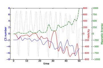
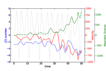
Figure 5: Plots of the Chern-Simons number (blue-dashed), magnetic helicity (red solid curve), and magnetic energy (green dot-dashed curve) for initial Chern-Simons number $n=1$ (top), $n=2$ (middle), and $n=3$ (bottom) in the second-order phase transition case. The kinetic energy of the Higgs is also shown in grey. Note the different scale bar for the EM energy shown in lattice units on the right-hand side of the plot.

The results for the second-order phase transition are very different from the results of the first-order phase transition. The oscillatory features can be understood by realizing that the Higgs field oscillates about the true minimum, as is clear from the oscillations in the Higgs kinetic energy curve in Fig. 5. We see the general feature that Chern-Simons number, magnetic helicity, and magnetic energy, all grow at late times, when the kinetic energy of the Higgs also starts dissipating. We can also understand the oscillatory behavior by noting that the Higgs field oscillates in the potential (light grey curve in in Fig. 5). The growth of the Chern-Simons number and magnetic helicity and energy, is more rapid for larger values of $n$. We expect the growth to saturate once the energy is evenly distributed between the scalar and gauge field sectors. However, to see this would require very long run times and very large lattices.

Our results show that even in the case of a second order phase transition, energy is transferred during the phase transition to EM magnetic fields with non-trivial helicity if the gauge fields initially have non-vanishing Chern-Simons number. As in the first-order phase transition case, the sign of magnetic helicity is the same as the sign of the change in Chern-Simons number.

III Conclusions

We have investigated the effects of pure gauge fields and their topology on the electroweak phase transition. The creation of magnetic fields from the gauge vacuum was anticipated in Ref. Jackiw and Pi (2000), treating the phase transition as a mathematical projection of the gauge fields into massive and massless components. In this paper we have numerically examined the classical dynamics of the electroweak symmetry breaking for different gauge vacua. Our results broadly agree with the analysis of Ref. Jackiw and Pi (2000) in that the evolution can lead to the creation of helical magnetic fields.

The details of the evolution are more involved. In the present work, we have explored the evolution and magnetic field generation during processes that can occur during a first-order phase transition that proceeds by bubble nucleation, and also during a second-order phase transition that proceeds by a continuously rolling Higgs field. In cases where the initial Chern-Simons number is zero and we set the gauge fields to zero, the evolution is trivial and the Chern-Simons number continues to be zero and magnetic fields are not produced. If the initial Chern-Simons number is non-zero but does not change during evolution (see the $n=1$ case in Fig. 1), even then helicity is not generated though magnetic fields are produced. This may be related to the generation of magnetic fields at the electroweak phase transition due to non-vanishing gradient energy of the Higgs as was discussed in Ref. Vachaspati (1991b, 1994). (For this reason we also expect magnetic fields to be produced in the zero Chern-Simons case if initially the gauge fields are not zero.) If the initial Chern-Simons number is large – greater than equal to 2 for the other parameters in our runs – the Chern-Simons number changes during evolution and magnetic helicity is produced. The connection between changes in the Chern-Simons number and magnetic helicity production, and the relation with changes in the baryon number via a quantum anomaly, has been pointed out in Refs. Cornwall (1997b); Vachaspati (2001b); Copi et al. (2008). Thus there are several lines of reasoning that point to the production of magnetic fields at the electroweak phase transition.

Based on early arguments we would expect that the magnetic helicity is directly proportional to the change in Chern-Simons number Cornwall (1997b); Vachaspati (2001b). In our runs, this simple relationship does not bear out. Instead we observe that the magnetic helicity goes as the square of the change in Chern-Simons number (Eq. (18)). This result should be considered tentative because we have only been able to run our simulations for a few values of the initial Chern-Simons number. Finer lattices and longer runs will be necessary to study a greater range of initial Chern-Simons number. Quantitative estimates of the magnetic field produced at the electroweak phase transition will require further work along the lines of Mou et al. (2017).

Finally we also mention that a non-Abelian vacuum consisting of a periodic array of pure gauge vortices has been proposed in Ref. Olesen (2016). It is argued that spontaneous symmetry breaking in such a vacuum can also generate magnetic fields Olesen (2017a, b). It would be worthwhile to study a dynamical phase transition in this vacuum just as we have done for the Chern-Simons vacua in this paper.

Appendix A Electroweak continuum equations

The classical electroweak equations of motion that result from the bosonic electroweak Lagrangian in Eq.(1) are:

$$D_{\mu}D^{\mu}\Phi+2\lambda(|\Phi|^{2}-\eta^{2})\Phi=0$$

$$\partial_{\mu}B^{\mu\nu}=g^{\prime}\text{Im}\big{[}\Phi^{\dagger}(D^{\nu}\Phi)\big{]}$$

$$\partial_{\mu}W^{a\mu\nu}+g\epsilon^{abc}W^{b}_{\mu}W^{c\mu\nu}=g\text{Im}\big{[}\Phi^{\dagger}\sigma^{a}(D^{\nu}\Phi)\big{]}.$$

In a numerical simulation, it is convenient to use the temporal gauge, $W_{0}^{a}=0$ and $B_{0}=0$. Then, the equations of motion become:

$$\partial_{0}^{2}\Phi\hphantom{{}_{i}}= D_{i}D_{i}\Phi-2\lambda(|\Phi|^{2}-\eta^{2})\Phi$$

$$\partial_{0}^{2}W^{a}_{i}= -\partial_{k}W^{a}_{ik}$$

$$-g\epsilon^{abc}W^{b}_{k}W^{c}_{ik}+g\text{Im}[\Phi^{\dagger}\sigma^{a}(D_{i}\Phi)]$$

$$\partial_{0}^{2}B_{i}= -\partial_{k}B_{ik}+g^{\prime}\text{Im}[\Phi^{\dagger}(D_{i}\Phi)],$$ (19)

along with two Gauss constraints,

$$\partial_{0}\partial_{j}B_{j}-g^{\prime}\text{Im}\big{[}\Phi^{\dagger}\partial_{0}\Phi\big{]}=0$$

$$\partial_{0}\partial_{j}W^{a}_{j}+g\epsilon^{abc}W^{b}_{j}\partial_{0}W^{c}_{j}-g\text{Im}\big{[}\Phi^{\dagger}\sigma^{a}\partial_{0}\Phi\big{]}=0.$$ (20)

We have implemented a discretized version of these equations following Ref. Vachaspati (2016) as a check of our main results that were obtained using the lattice formulation of Appendix B.

Appendix B Lattice implementation

Our lattice implementation of the electroweak evolution equations follows closely the discussion in Ref. Rajantie et al. (2001).

We introduce the lattice based fields $U_{\mu}(t,x)$ and $V_{\mu}(t,x)$, which are related to the continuum gauge fields through:

$$U_{i}(t,x) = \exp{\Big{(}-\frac{i}{2}g\Delta x\sigma^{a}W^{a}_{i}\Big{)}}$$

$$U_{0}(t,x) = \exp{\Big{(}-\frac{i}{2}g\Delta t\sigma^{a}W^{a}_{0}\Big{)}}$$

$$V_{i}(t,x) = \exp{\Big{(}-\frac{i}{2}g\Delta xB_{i}\Big{)}}$$

$$V_{0}(t,x) = \exp{\Big{(}-\frac{i}{2}g\Delta tB_{0}\Big{)}}.$$ (21)

The discretized action in terms of these fields is:

$$S = \sum_{x,t}\Delta t\Delta x^{3}\Bigg{\{}\big{(}D_{0}\Phi\big{)}^{\dagger}\big{(}D_{0}\Phi\big{)}-\sum_{i}\big{(}D_{i}\Phi\big{)}^{\dagger}\big{(}D_{i}\Phi\big{)}-U(\Phi)+\Big{(}\frac{2}{g\Delta t\Delta x}\Big{)}^{2}\sum_{i}\Big{(}1-\frac{1}{2}\text{Tr}~{}U_{0i}\Big{)}$$ (22)

$$+\Big{(}\frac{2}{g^{\prime}\Delta t\Delta x}\Big{)}^{2}\sum_{i}\Big{(}1-\text{Re}~{}V_{0i}\Big{)}-\frac{2}{g^{2}\Delta x^{4}}\sum_{i,j}\Big{(}1-\frac{1}{2}\text{Tr}~{}U_{ij}\Big{)}-\frac{2}{g^{\prime 2}\Delta x^{4}}\sum_{i,j}\Big{(}1-\text{Re}~{}V_{ij}\Big{)}\Bigg{\}},$$

where, $\Phi(t,x)$ is the Higgs field doublet defined on each lattice site; $U_{i}(t,x)$ and $V_{i}(t,x)$ are the SU(2) and U(1) link fields, respectively, defined on the link between the neighboring sites $x$ and $x+i$; and for the U(1) link field we take the real part rather than the trace as in Ref. Rajantie et al. (2001). Also, $U_{0}(t,x)=I_{2}$ and $V_{0}(t,x)=1$ consistent with (21) and our choice of temporal gauge. Note that throughout this appendix Latin indices take values $i,j,k=1,2,3$ and repeated indices are not summed over.

Here, we adopt the conventional interpretation that $U_{i}(t,x)$, $V_{i}(t,x)$ parallel transport the fields at site $x+i$ back to site $x$; then $U_{i}^{\dagger}(t,x)$, $V_{i}^{\dagger}(t,x)$ parallel transport the fields at site $x$ to $x+i$. Then, the covariant derivative of $\Phi(t,x)$ that enters in Eq. (22) has components:

$$D_{i}\Phi =\frac{1}{\Delta x}\big{[}U_{i}(t,x)V_{i}(t,x)\Phi(t,x+i)-\Phi(t,x)\big{]}$$

$$D_{0}\Phi =\frac{1}{\Delta t}\big{[}U_{0}(t,x)V_{0}(t,x)\Phi(t+\Delta t,x)-\Phi(t,x)\big{]}.$$

Finally, the plaquette fields can be seen as the discretized version of the magnetic fields:

$$U_{ij}(t,x)=U_{j}(t,x)U_{i}(t,x+j)U_{j}^{\dagger}(t,x+i)U_{i}^{\dagger}(t,x)$$

$$V_{ij}(t,x)=V_{j}(t,x)V_{i}(t,x+j)V_{j}^{\dagger}(t,x+i)V_{i}^{\dagger}(t,x).$$

The fields $\Phi(t,x)$, $U_{i}(t,x)$ and $V_{i}(t,x)$ are defined at the time steps $t+\Delta t$, $t+2\Delta t$, $\ldots$; while the conjugate momentum fields, $\Pi(t+\Delta t/2,x)$, $F(t+\Delta t/2,x)$ and $E(t+\Delta t/2,x)$, are defined at time steps $t+\Delta t/2$, $t+3\Delta t/2$, $\ldots$. They are related by

$$\Phi(t+\Delta t,x)= \Phi(t,x)+\Delta t\Pi(t+\Delta t/2,x)$$ (23)

$$V_{i}(t+\Delta t,x)= \frac{1}{2}g^{\prime}\Delta x\Delta tE_{i}(t+\Delta t/2,x)V_{i}(t,x)$$ (24)

$$U_{i}(t+\Delta t,x)= g\Delta x\Delta tF_{i}(t+\Delta t/2,x)U_{i}(t,x),$$ (25)

The equations of motion that result from setting the functional derivative of the action to zero are:

$$\Pi(t+\Delta t/2,x)= \Pi(t-\Delta t/2,x)+\Delta t\Big{\{}\frac{1}{\Delta x^{2}}\sum_{i}\big{[}U_{i}(t,x)V_{i}(t,x)\Phi(t,x+i)$$

$$-2\Phi(t,x)+U_{i}^{\dagger}(t,x-i)V_{i}^{\dagger}(t,x-i)\Phi(t,x-i)\big{]}-\frac{\partial U}{\partial\Phi^{\dagger}}\Big{\}}$$ (26)

$$\text{Im}[E_{k}(t+\Delta t/2,x)]= \text{Im}[E_{k}(t-\Delta t/2,x)]+\Delta t\Big{\{}\frac{g^{\prime}}{\Delta x}\text{Im}[\Phi^{\dagger}(t,x+k)U^{\dagger}_{k}(t,x)V^{\dagger}_{k}(t,x)\Phi(t,x)]$$

$$-\frac{2}{g^{\prime}\Delta x^{3}}\sum_{i}\text{Im}[V_{k}(t,x)V_{i}(t,x+k)V_{k}^{\dagger}(t,x+i)V_{i}^{\dagger}(t,x)$$

$$+V_{i}(t,x-i)V_{k}(t,x)V_{i}^{\dagger}(t,x+k-i)V_{k}^{\dagger}(t,x-i)]\Big{\}}$$ (27)

$$\text{Tr}[i\sigma^{m}F_{k}(t+\Delta t/2,x)]= \text{Tr}[i\sigma^{m}F_{k}(t-\Delta t/2,x)]+\Delta t\Big{\{}\frac{g}{\Delta x}\text{Re}[\Phi^{\dagger}(t,x+k)U_{k}^{\dagger}(t,x)V_{k}^{\dagger}(t,x)i\sigma^{m}\Phi(t,x)]$$

$$-\frac{1}{g\Delta x^{3}}\sum_{i}\text{Tr}[i\sigma^{m}U_{k}(t,x)U_{i}(t,x+k)U_{k}^{\dagger}(t,x+i)U_{i}^{\dagger}(t,x)$$

$$+i\sigma^{m}U_{k}(t,x)U_{i}^{\dagger}(t,x+k-i)U_{k}^{\dagger}(t,x-i)U_{i}(t,x-i)]\Big{\}},$$ (28)

where, in Eq. (26) the term $U_{i}^{\dagger}(t,x-i)V_{i}^{\dagger}(t,x-i)\Phi(t,x-i)$ corrects the corresponding equation (A17) in Ref. Rajantie et al. (2001) where it is written without the $-i$. The remaining components, $\text{Re}(E_{k})$ and $\text{Tr}(F_{k})$, can be found by using:

$$|E|=\frac{2}{g^{\prime}\Delta x\Delta t},\quad\text{det}(F)=\Big{(}\frac{1}{g\Delta x\Delta t}\Big{)}^{2},$$ (29)

where the square in the second equation corrects a typo in Ref. Rajantie et al. (2001).

The lattice action (22) is invariant under gauge transformations:

$$\Phi(t,x) \rightarrow\Omega_{1}(t,x)\Omega_{2}(t,x)\Phi(t,x)$$

$$U_{i}(t,x) \rightarrow\Omega_{2}(t,x)U_{i}(t,x)\Omega_{2}^{\dagger}(t,x+i)$$

$$V_{i}(t,x) \rightarrow\Omega_{1}(t,x)V_{i}(t,x)\Omega_{1}^{\dagger}(t,x+i)$$

$$\Omega_{2} \in SU(2),\quad\Omega_{1}\in U(1),$$

which imply the following Gauss constraints:

$$G_{\rm U1}(x)\equiv\frac{1}{\Delta x}\sum_{i}\text{Im}[E_{i}(t+\Delta t/2,x)-E_{i}(t+\Delta t/2,x-i)]-g^{\prime}\text{Im}[\Pi^{\dagger}(t+\Delta t/2,x)\Phi(t,x)] = 0$$ (30)

$$G_{\rm SU2}^{k}(x)\equiv\frac{1}{\Delta x}\sum_{i}\text{Tr}~{}\{i\sigma^{k}\big{[}F_{i}(t+\Delta t/2,x)-U_{i}^{\dagger}(t,x-i)F_{i}(t+\Delta t/2,x-i)U_{i}(t,x-i)\big{]}\}$$

$$-g\text{Re}[\Pi^{\dagger}(t+\Delta t/2,x)i\sigma^{k}\Phi(t,x)] = 0$$ (31)

If the initial time is $t_{0}=0$, our initial conditions should specify $\Phi(0,x)$, $U_{i}(0,x)$, $V_{i}(0,x)$, as well as $\Pi(\Delta t/2,x)$, $F_{i}(\Delta t/2,x)$, $E_{i}(\Delta t/2,x)$. This is consistent with the requirements for second-order differential equations. As mentioned in Moore (1996), there is no conserved quantity that can be identified as energy, but we can construct a quantity that approaches the conserved energy in the small $\Delta t$ limit:

$$E = \sum_{x}\Delta x^{3}\Bigg{\{}\Big{(}\frac{\Pi(t+\Delta t/2,x)+\Pi(t-\Delta t/2,x)}{2}\Big{)}^{\dagger}\Big{(}\frac{\Pi(t+\Delta t/2,x)+\Pi(t-\Delta t/2,x)}{2}\Big{)}$$ (32)

$$+\sum_{i}\big{[}D_{i}\Phi(t,x)\big{]}^{\dagger}\big{[}D_{i}\Phi(t,x)\big{]}+U(\Phi(t,x))$$

$$+\Big{(}\frac{2}{g\Delta t\Delta x}\Big{)}^{2}\frac{1}{2}\sum_{i}\Big{[}\Big{(}1-\frac{g\Delta x\Delta t}{2}\text{Tr}~{}F_{i}(t+\Delta t/2,x)\Big{)}+\Big{(}1-\frac{g\Delta x\Delta t}{2}\text{Tr}~{}F_{i}(t-\Delta t/2,x)\Big{)}\Big{]}$$

$$+\Big{(}\frac{2}{g^{\prime}\Delta t\Delta x}\Big{)}^{2}\frac{1}{2}\sum_{i}\Big{[}\Big{(}1-\frac{g^{\prime}\Delta x\Delta t}{2}\text{Re}~{}E_{i}(t+\Delta t/2,x)\Big{)}+\Big{(}1-\frac{g^{\prime}\Delta x\Delta t}{2}\text{Re}~{}E_{i}(t-\Delta t/2,x)\Big{)}\Big{]}$$

$$+\frac{2}{g^{2}\Delta x^{4}}\sum_{i,j}\Big{(}1-\frac{1}{2}\text{Tr}~{}U_{ij}(t,x)\Big{)}+\frac{2}{g^{\prime 2}\Delta x^{4}}\sum_{i,j}\Big{(}1-\text{Re}~{}V_{ij}(t,x)\Big{)}\Bigg{\}}$$

There are two checks that can be made to ensure the simulation is running correctly. The first one is conservation of total energy. Given a localized configuration, the total energy inside the lattice box should be fixed before this configuration reaches the boundary. The second check is that the Gauss constraints should be satisfied. Following Ref. Rajantie et al. (2001), we introduce a “Hamiltonian”

$$H=\frac{(\Delta x)^{3}}{2}\sum_{x}[G_{\rm U1}(x)G_{\rm U1}(x)+G_{\rm SU2}^{k}(x)G_{\rm SU2}^{k}(x)]$$ (33)

as a measure of the violation of the Gauss constraints. Numerically, the value of Eq. (33) should be very close to zero. As pointed out in Moore (1996), the Gauss constraints are preserved by the evolution algorithm as long as they are satisfied by the initial conditions. However, we are using ABC to evolve the fields at the boundaries. The ABC equations, discussed in the following appendix, do not in general preserve the Gauss constraints. We find that our simulations satisfy the constraints to a very high accuracy, which is a non-trivial check that the boundary conditions are appropriate.

Appendix C Absorbing Boundary Conditions

To implement absorbing boundary conditions in our simulations, we extend the results in Engquist and Majda (1977); Szeftel (2006); Feng (1999) as described below.

Neglecting for the moment interactions with gauge fields, the equation of motion for the Higgs can be written as

$$[\partial_{t}^{2}-\nabla^{2}+J(\Phi)]\Phi=0,$$ (34)

where $J(\Phi)=2\lambda(|\Phi|^{2}-\eta^{2})$.

We can formally decompose Eq.(34) at a boundary as

$$\big{[}\bm{n}\cdot\nabla-\sqrt{\partial_{t}^{2}-\partial_{\perp}^{2}+J(\Phi)}\big{]}\big{[}\bm{n}\cdot\nabla+\sqrt{\partial_{t}^{2}-\partial_{\perp}^{2}+J(\Phi)}\big{]}\Phi=0,$$ (35)

where $\bm{n}$ is the outward pointing unit normal vector of the boundary, and $\partial_{\perp}\equiv\nabla-\bm{n}(\bm{n}\cdot\nabla)$.

To prevent exterior waves from entering the simulation lattice, while allowing outgoing waves to leave the box, we require

$$\big{[}\bm{n}\cdot\nabla+\sqrt{\partial_{t}^{2}-\partial_{\perp}^{2}+J(\Phi)}\big{]}\Phi=0.$$ (36)

To find a local approximate form of Eq.(36) that is suitable for numerical implementation, we need to expand the square root in a power series.

If $\partial_{t}^{2}$ is the dominant term, then $-\partial_{\perp}^{2}+J(\Phi)$ can be treated as a small perturbation. This approximation will be most accurate for waves that hit the boundary perpendicularly, with negligible $\partial_{\perp}^{2}\Phi$ and negligible $J(\Phi)$. Keeping terms that are linear in the perturbation, Eq.(36) becomes

$$\Bigg{[}\bm{n}\cdot\nabla+\partial_{t}\bigg{(}1-\frac{\partial_{\perp}^{2}-J(\Phi)}{2\partial_{t}^{2}}\bigg{)}\Bigg{]}\Phi=0,$$ (37)

which can be simplified as

$$\partial_{t}^{2}\Phi=-\bm{n}\cdot\nabla\partial_{t}\Phi+\frac{1}{2}\partial_{\perp}^{2}\Phi-\frac{1}{2}J(\Phi)\Phi.$$ (38)

We use this approximation when simulating a first-order phase transition, as $J(\Phi)$ can then be neglected at the boundary.

In the case of a second-order phase transition, even for $t=0$ the potential is not small at the boundary. Therefore we treat $\partial_{t}^{2}+J(\Phi)$ as the dominant term and $\partial_{\perp}^{2}$ as a perturbation. Now Eq.(36) becomes

$$\Bigg{[}\bm{n}\cdot\nabla+\sqrt{\partial_{t}^{2}+J(\Phi)}\bigg{(}1-\frac{\partial_{\perp}^{2}}{2(\partial_{t}^{2}+J(\Phi))}\bigg{)}\Bigg{]}\Phi=0$$ (39)

Assuming that $\partial_{t}^{2}\gg J(\Phi)\gg\partial_{\perp}^{2}$, we can further simplify the above equation as

$$\partial_{t}^{2}\Phi=-\bm{n}\cdot\nabla\partial_{t}\Phi+\frac{1}{2}\partial_{\perp}^{2}\Phi-J(\Phi)\Phi.$$ (40)

Although this scheme can be extended to include higher order terms in the perturbation, we find that Eqs. (38) and (40) are accurate enough for our purpose.

To take into account the coupling of the Higgs to the gauge fields, the spatial derivatives in Eq.(34) should be replaced with covariant derivatives. We start by writing Eq.(34) as

$$[\partial_{t}^{2}-\nabla^{2}+\nabla^{2}-D^{2}+J(\Phi)]\Phi=0,$$ (41)

where $D$ denotes the covariant derivative. Then the previous discussion still holds if we use the current $J^{\prime}(\Phi)\equiv\nabla^{2}-D^{2}+J(\Phi)$, which now includes the gauge interactions.

To evolve the gauge fields at the boundary, we use the lowest order absorbing boundary conditions:

$$\bm{E}^{T}=-\bm{n}\times\bm{B}$$ (42)

In principle, higher order corrections could be included along similar lines as for the scalar wave equation. However, it has been argued in Feng (1999) that they may give rise to numerical instabilities.

We stress that implementing the ABC for gauge fields on the lattice requires us to make some compromises that cannot always be rigorously justified. We use a scheme that only requires two time slices and the nearest neighboring spatial points, which roughly speaking is robust as long as the gauge fields on the boundary are small. As shown by the energy and Gauss constraint checks, they are adequate for our purposes.

References

- Sakharov (1967) A. D. Sakharov, JETP lett. 5, 24 (1967).
- Cornwall (1997a) J. M. Cornwall, Physical Review D 56, 6146 (1997a).
- Vachaspati (2001a) T. Vachaspati, Physical review letters 87, 251302 (2001a).
- Manton (1983) N. S. Manton, Phys. Rev. D28, 2019 (1983).
- Vachaspati and Field (1994) T. Vachaspati and G. B. Field, Physical review letters 73, 373 (1994).
- Hindmarsh and James (1994) M. Hindmarsh and M. James, Physical Review D 49, 6109 (1994).
- Saurabh and Vachaspati (2017) A. Saurabh and T. Vachaspati (2017), eprint 1705.03091.
- Copi et al. (2008) C. J. Copi, F. Ferrer, T. Vachaspati, and A. Achúcarro, Physical review letters 101, 171302 (2008).
- Chu et al. (2011) Y.-Z. Chu, J. B. Dent, and T. Vachaspati, Physical Review D 83, 123530 (2011).
- Jackiw and Pi (2000) R. Jackiw and S.-Y. Pi, Physical Review D 61, 105015 (2000).
- Vachaspati (1991a) T. Vachaspati, Physics Letters B 265, 258 (1991a).
- Rajantie et al. (2001) A. Rajantie, P. Saffin, and E. J. Copeland, Physical Review D 63, 123512 (2001).
- Vachaspati (2016) T. Vachaspati, Phys. Rev. Lett. 117, 181601 (2016), eprint 1607.07460.
- Klinkhamer and Manton (1984) F. R. Klinkhamer and N. S. Manton, Phys. Rev. D30, 2212 (1984).
- Vachaspati (1991b) T. Vachaspati, Phys. Lett. B265, 258 (1991b).
- Vachaspati (1994) T. Vachaspati, in Sintra Electroweak 1994:171-184 (1994), pp. 171–184, eprint hep-ph/9405286, URL http://alice.cern.ch/format/showfull?sysnb=0181105.
- Cornwall (1997b) J. M. Cornwall, Phys. Rev. D56, 6146 (1997b), eprint hep-th/9704022.
- Vachaspati (2001b) T. Vachaspati, Phys. Rev. Lett. 87, 251302 (2001b), eprint astro-ph/0101261.
- Mou et al. (2017) Z.-G. Mou, P. M. Saffin, and A. Tranberg (2017), eprint 1704.08888.
- Olesen (2016) P. Olesen (2016), eprint 1605.00603.
- Olesen (2017a) P. Olesen (2017a), eprint 1701.00245.
- Olesen (2017b) P. Olesen (2017b), eprint 1705.02055.
- Moore (1996) G. D. Moore, Nuclear Physics B 480, 689 (1996).
- Engquist and Majda (1977) B. Engquist and A. Majda, Proceedings of the National Academy of Sciences 74, 1765 (1977).
- Szeftel (2006) J. Szeftel, Mathematics of computation 75, 565 (2006).
- Feng (1999) X. Feng, Mathematics of Computation of the American Mathematical Society 68, 145 (1999).