Renormalization in a Lorentz-violating model and higher-order operators

Abstract

The renormalization in a Lorentz-breaking scalar-spinor higher-derivative model involving $\phi^{4}$ self-interaction and the Yukawa-like coupling is studied. We explicitly de- monstrate that the convergence is improved in comparison with the usual scalar-spinor model, so, the theory is super- renormalizable, with no divergences beyond four loops. We compute the one-loop corrections to the propagators for the scalar and fermionic fields and show that in the presence of higher-order Lorentz invariance violation, the poles that dominate the physical theory, are driven away from the standard on-shell pole mass due to radiatively induced lower dimensional operators. The new operators change the standard gamma-matrix structure of the two-point functions, introduce large Lorentz-breaking corrections and lead to modifications in the renormalization conditions of the theory. We found the physical pole mass in each sector of our model.

1 Introduction

It is well known that the Lorentz-breaking field theory models can be introduced in several ways. We can list some of the most popular approaches. First, one can introduce small Lorentz-breaking modifications of the known theories through additive terms, thus implementing the Lorentz-breaking extensions of the standard model ColKost . In principle, the most known extensions of the QED follow this way. A very extensive list of the possible Lorentz-breaking additive terms in different field theory models including QED is given by KosGra . Second, one can start with the modified dispersion relations Amelino , and, in principle, try to find a theory yielding such relations. Third, the Lorentz-breaking theories can be treated as a low-energy limit of some fundamental theories, for example string theory KostSam and loop quantum gravity LQG . Finally, the Lorentz symmetry can be broken spontaneously, see f.e. spont . The main motivation behind all these approaches, however, is the same, and resides in the expectation that any experimental evidence of departure from Lorentz symmetry may provide the first germs towards the construction of a theory amalgamating both General Relativity and the Standard Model of particle physics.

At the same time, it is natural to consider one more aspect of studying the Lorentz-breaking extensions of the field theory models. It consists in introducing essentially Lorentz- breaking terms, that is, those ones proportional to some constant vectors or tensors, involving higher derivatives. As a result, the corresponding theory will yield an essentially different quantum dynamics. The first known example of such a theory is the Myers-Pospelov extension of the electrodynamics MP where the three-derivative term essentially involves the Lorentz symmetry breaking. Another important example of such a theory is the four-dimensional Chern-Simons modified gravity with the Chern-Simons coefficient chosen in special form $\Theta(x)=k_{\mu}x^{\mu}$ JaPi , which, in the weak field limit, also involves third order in derivatives of the dynamical field (that is, the metric fluctuation). Moreover, the importance of the Myers-Pospelov-like term, and analogous terms for scalar and spinor fields which can be easily introduced, is also motivated by the fact that a special choice of the Lorentz-breaking vector will allow to eliminate the presence of higher time derivatives thus avoiding the arising of the ghosts which are typically present in theories with higher time derivatives (see f.e. ghosts ). Also, this term was shown to arise as a quantum correction in different Lorentz-breaking extensions of QED MNP and has been studied for causality and stability CMR0 . In the case of including higher time derivatives, it has been shown recently that the unitarity of the $S$-matrix can be preserved at the one-loop order in a Myers-Pospelov QED CMR . The proof has been accomplished using the Lee-Wick prescription for quantum field theories with negative metric Lee-Wick . For other studies on unitarity at tree level for minimal and nonminimal Lorentz violations, see Schreck1 ; Schreck2 respectively. It is important to notice that the Myers-Pospelov-like modifications of QED are actually experimentally studied as well within different contexts MPexp .

We emphasize that, up to now, the quantum impact of the Myers-Pospelov-like class of terms being introduced already at the classical level, where the higher-derivative additive term should carry a small parameter which can enforce large quantum corrections collins , almost was not studied except of the QED Fine-Tuning and superfield case CMP . The presence of such effect raises the question how to define correctly the physical parameters in the renormalized theory. On the other hand, for studies in the context of semiclassical quantization it is natural to consider the presence of higher derivative terms in order to implement a consistent renormalization program shapiro . With these considerations, the natural question is – what are the possible consequences of including the Lorentz-breaking higher-derivative terms into the classical action?

It is well known that loop corrections in Lorentz- violating quantum field theory may lead to new kinetic operators absent in the original Lagrangian. Recently, the consequences of these radiatively induced operators have been studied in relation with the finiteness of the $S$-matrix and the identification of the asymptotic state space ralf . These new terms introduce modifications in the propagation of free particles and change drastically the physical content of the space of in and out states. In particular, the Källén–Lehmann representation KL and the Lehmann- Symanzik- Zimmermann (LSZ) reduction formalism LSZ are modified in the presence of Lorentz symmetry violation rob . An important finding is that spectral densities which in the standard case are functions of momentum-dependent observer scalars such as $p^{2}$, in the Lorentz violating scenario may depend on other scalars such as couplings of Lorentz-violating tensor coefficients with momenta rob . This has led to modifications in the renormalization procedure, in the definition of the asymptotic Hilbert space and in general in the treatment for external-leg physics ralf ; for other studies of the renormalization in Lorentz-breaking theories, see also scarp . A natural extension for these studies is to consider the nonminimal framework of Lorentz invariance violation, that is, when the Lorentz-breaking is performed with higher-order operators Kos-Mew . It is well known that the inclusion of higher-order operators in quantum field theory will generate, via radiative corrections, all the lower dimensional operators allowed by the symmetries of the Lagrangian gen_rad . For the case of breaking the Lorentz symmetry, let us say in QED and with a preferred four-vector $n^{\mu}$, the induced operators may involve contractions of $n_{\mu}$ with matrices other than just $\gamma^{\mu}$, together with scalars such as $(n\cdot p)$. The new terms force to modify the renormalization conditions in order to extract the correct pole mass from the two-point functions. In particular, the renormalization condition for the renormalized fermion self-energy $\Sigma_{R}(\not{p}=m_{P})=0$, with $m_{P}$ being the physical pole mass, has to be generalized, which ultimately will depend on the form of Lorentz breaking. In this work we continue these studies in order to carry out the renormalization in a theory with higher-order operators and in addition we study the possible effects of large Lorentz-violating corrections. Within our study, we consider the renormalization of the higher-derivative Lorentz-breaking generalizations of $\lambda\phi^{4}$ and Yukawa model.

The structure of the paper looks like follows. In Sec. 2, we consider the classical actions of our models, write down the dispersion relations, find the poles and describe their analytical behavior in complex $p_{0}$-plane. In Sec. 3, we compute the quantum corrections corresponding to the self interaction $\lambda\phi^{4}$. In Sec. 4 we discuss the coupling of scalar and spinor fields and provide a study of the degree of divergencies in our model. In Sec. 5, we compute the two-point functions in purely scalar and scalar-spinor sectors thus exhausting possible divergences and showing explicitly the radiatively induced operators with new gamma-matrix structure and large Lorentz-violating terms. In Sec. 6, we perform the mass renormalization in both sectors and find the physical masses in the theory. In the last section, we discuss our results, and in the Appendices A, B and C, we provide some details of the calculations.

2 The effective models and pole structure

We are interested in the higher-order Lagrangian density describing two sectors of Lorentz-breaking theory

$$\mathcal{L}=\mathcal{L}_{1}+\mathcal{L}_{2}\,.$$ (1)

The first sector involves a scalar sector with a fourth derivative together with a self-interaction potential term

$$\mathcal{L}_{1}=\frac{1}{2}\partial_{\mu}\phi\partial^{\mu}\phi-\frac{1}{2}M^{2}\phi^{2}+g_{1}\phi(n\cdot\partial)^{4}\phi-\frac{\lambda}{4!}\phi^{4}\,,$$ (2)

and the second one the fermionic Myers-Pospelov model MP , with dimension-five operators and the Yukawa coupling vertex

$${\cal L}_{2}=\bar{\psi}\left(i\partial\!\!\!/-m-\bar{\alpha}mn\!\!\!/\right)\psi+g_{2}\bar{\psi}n\!\!\!/(n\cdot\partial)^{2}\psi+g\bar{\psi}\phi\psi\,.$$ (3)

The constants $g_{1}=\frac{\kappa}{M^{2}_{Pl}}$ and $g_{2}=\frac{\eta}{M_{Pl}}$ parametrize the higher-order Lorentz invariance violation with $M_{P}$ the Planck mass representing itself as a natural mass scale, $\kappa$, $\eta$ and $\bar{\alpha}$ are dimensionless parameters, whose presence describes the intensity of the higher-derivative terms, and $n^{\mu}$ is a dimensionless four-vector defining a preferred reference frame.

Figure 1: The path of integration $C_{F}^{(s)}$ for the scalar propagator which encloses the poles $-p_{1}$ and $iP_{2}$ when closing the contour upward and encloses the poles $p_{1}$ and $-iP_{2}$ when closing the contour downward.

The propagators in momentum space read

$$\Delta(p) = \frac{i}{p^{2}-M^{2}+2g_{1}(n\cdot p)^{4}}\,,$$

$$S(p) = \frac{i}{p\!\!\!/-m-\bar{\alpha}mn\!\!\!/-g_{2}n\!\!\!/(n\cdot p)^{2}}\,.$$ (4)

We begin an analysis of the dispersion relations in both sectors. A further motivation for its study, and consequently, the finding of the poles and their analytical behavior in complex $p_{0}$-plane, consists first in the fact that in our models namely using of the residues of the propagators is a most convenient approach for calculating the quantum corrections. Second, in the presence of higher-order time-derivative terms a direct implementation of the $i\epsilon$ prescription may lead to a wrong four-momentum representation for the propagator which may spoil any attempt to preserve unitarity or causality.

Let us start with the scalar dispersion relation, namely

$$p^{2}-M^{2}+2g_{1}(n\cdot p)^{4}=0\,,$$ (5)

which for a purely time-like four-vector $n^{\mu}=(1,0,0,0)$, the solutions are given by

$$p_{0}=\pm\frac{1}{2}\sqrt{\frac{-1\pm\sqrt{1+8g_{1}E^{2}}}{g_{1}}},$$ (6)

and where $E(\vec{p})=\sqrt{{\vec{p}}^{2}+M^{2}}$. The dispersion relation can also be written as $(p_{0}^{2}-p_{1}^{2})(p_{0}^{2}+P_{2}^{2})=0$, hence one has the solutions $p_{0}=\pm p_{1}$ and $p_{0}=\pm iP_{2}$ so that

$$p_{1} = \frac{1}{2}\sqrt{\frac{-1+\sqrt{1+8g_{1}E^{2}}}{g_{1}}}\,,$$

$$P_{2} = \frac{1}{2}\sqrt{\frac{1+\sqrt{1+8g_{1}E^{2}}}{g_{1}}}\,.$$ (7)

Their exact location in complex $p_{0}$-plane and also the contour of integration $C_{F}^{(s)}$ are shown in Fig. 1.

The solutions can be classified according to their perturbative behavior when taking the Lorentz violation to zero. We identify two standard solutions $\pm p_{1}$ which are perturbative solutions to the usual ones $\pm E$ and two complex ones (and moreover, actually tachyonic) $\pm iP_{2}$ which diverge as $g_{1}\to 0$. The extra solutions that appear $\pm P_{2}$ are associated to negative-metric states in Hilbert space and have been called Lee-Wick solutions Lee-Wick .

Figure 2: The integration contour $C_{F}^{(f)}$ for the fermion propagator which is defined to round the negative pole from below and the positive poles from above. At higher energies than $1/(4g_{2})$, the two solutions $\omega_{1}$ and $W_{1}$ become complex and move in opposite directions along the imaginary line starting at $1/(2g_{2})$, we deform the contour continuously avoiding any crossing or singularity with the poles.

Alternatively, we can write the scalar propagator as

$$\Delta(p) = \frac{i}{2g_{1}(p_{0}^{2}+P_{2}^{2})(p_{0}^{2}-p_{1}^{2}+i\epsilon)}\,,$$ (8)

which agrees with the usual propagator in the limit $g_{1}\to 0$.

In the fermion sector we have the dispersion relation

$$(p_{\mu}-\bar{\alpha}mn_{\mu}-g_{2}n_{\mu}(n\cdot p)^{2})^{2}-m^{2}=0\,.$$ (9)

Again for the time-like $n^{\mu}$ we have the equation

$$(p_{0}-\bar{\alpha}m-g_{2}p_{0}^{2})^{2}-\vec{p}^{2}-m^{2}=0\,,$$ (10)

whose standard, that is, non-singular at $g_{2}\to 0$, solutions are

$$\omega_{1} = \frac{1-\sqrt{1-4g_{2}(\bar{\alpha}m+\mathcal{E})}}{2g_{2}}$$

$$\omega_{2} = \frac{1-\sqrt{1+4g_{2}(\mathcal{E}-\bar{\alpha}m)}}{2g_{2}}\,,$$ (11)

and the Lee-Wick ones

$$W_{1} = \frac{1+\sqrt{1-4g_{2}(\bar{\alpha}m+\mathcal{E})}}{2g_{2}}$$

$$W_{2} = \frac{1+\sqrt{1+4g_{2}(\mathcal{E}-\bar{\alpha}m)}}{2g_{2}}\,,$$ (12)

where $\mathcal{E}(\vec{p})=\sqrt{\vec{p}^{2}+m^{2}}$.

In the region of energies satisfying the condition $4g_{2}(\mathcal{E}\pm\bar{\alpha})<1$ the four solutions are real and obey the inequality $\omega_{2}<\omega_{1}<W_{1}<W_{2}$ at least for $\bar{\alpha}$ enough small, where $\omega_{2}$ is a negative number. However, beyond the critical energy $1/(4g_{2})$ both $\omega_{1}$ and $W_{1}$ become complex and move in the opposite imaginary line at $1/(2g_{2})$ as shown in Fig. 2, while the other two solutions $\omega_{2},W_{2}$ remain real.

To define the contour $C_{F}^{(f)}$ we use an heuristic argument, specially to go beyond the critical energy at which complex solutions appear. We implement a correct low energy limit by considering the prescription given in QEDunitarity which has been well tested to give a suitable correspondence with the normal theory when $g_{2}\to 0$ and also to preserve the unitarity of the $S$ matrix. In this effective region the integration contour $C_{F}^{(f)}$ is defined to round the negative pole from below and the three positive ones from above. Now we increase the energy to values at which the two solutions $\omega_{1}$ and $W_{1}$ become complex, and define the new contour as the one obtained by continuously deforming the curve by avoiding any crossing and singularity with the poles, as shown in Fig. 2.

With this consideration in mind, the fermion propagator reads

$$S(p) = \frac{i\left((p_{0}-\bar{\alpha}m-g_{2}p_{0}^{2})\gamma^{0}+p_{i}\gamma^{i}+m\right)}{g_{2}^{2}(p_{0}-\omega_{1}+i\epsilon)(p_{0}-W_{1}+i\epsilon)(p_{0}-\omega_{2}-i\epsilon)}$$ (13)

$$\times \frac{1}{(p_{0}-W_{2}+i\epsilon)}\,,$$

which differs from the direct $i\epsilon$ prescription in the quadratic terms, but allows in particular to define a consistent Wick rotation which we use later.

3 The interaction $\lambda\phi^{4}$

In this section we explore the potentially divergent one-loop radiative correction in the scalar propagator which is generated by the well-known tadpole graph given by Fig. 3.

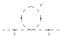
Figure 3: One-loop graph in the scalar model with self interaction $\lambda\phi^{4}$.

To proceed with it, we need to evaluate the basic integral

$$\Sigma_{2}=\frac{1}{2}\lambda\int\frac{d^{4}p}{(2\pi)^{4}}\frac{1}{p^{2}-M^{2}+2g_{1}(n\cdot p)^{4}}\,.$$ (14)

with some regularization technique.

Before computing the above integral, let us comment on the well known fact that perturbative approximation for physical observables can show some ambiguities depending on the regularization scheme. This brief detour will give us some insight of the finite nature of some integrals which we will compute using the scheme of analytic continuation to $d$ dimensions or dimensional regularization (DR).

To be more clear, let us consider the integral $\Sigma_{2}$ in the standard case (taking $g_{1}\to 0$), for which we will arrive to the well known expression in dimensional regularization

$$\Sigma_{2}^{\rm DR}=\frac{i\lambda M^{2}}{16\pi^{2}\epsilon}+\rm{fin}.$$ (15)

On the other hand, using a cutoff regularization in which we introduce an upper limit in momenta proportional to $\Lambda$ will produce

$$\Sigma_{2}^{\rm cut-off}=\frac{\Lambda^{2}}{2}-\frac{M^{2}}{4}\left(2\ln\left(\frac{2\Lambda}{M}\right)-1\right)+\mathcal{O}(\Lambda^{-2})\,,$$ (16)

which includes quadratic and logarithmic divergencies.

These two results not only show the ambiguity of results for observables in the perturbative scheme, but also the important fact that quadratic divergencies are not seen by dimensional regularization which only has the property to describe logarithmic divergences. In our case something similar happens. As we will show in the Appendix C, some of our integrals display divergences proportional to powers of $\Lambda$ with the absence of logarithmic divergences, and hence dimensional regularization will give finite results for these integrals.

We return to the computation of $\Sigma_{2}$. We use DR and go to $d$ dimensions and choose the Lorentz-breaking four-vector to be timelike $n^{\mu}=(1,0,0,0)$ which yields

$$\Sigma_{2} = \frac{1}{2}\mu^{4-d}\lambda\int\frac{d^{d}p}{(2\pi)^{d}}\frac{1}{2g_{1}(p_{0}^{2}-p_{1}^{2}+i\epsilon)(p_{0}^{2}+P_{2}^{2})}\,,$$ (17)

where $p_{1},P_{2}$ are given in (2). We perform the integration in the complex $p_{0}$-plane by closing the contour $C_{F}^{(s)}$ upward and enclosing the two poles $-p_{1}$ and $iP_{2}$ as depicted in Fig. 1, yielding

$$\Sigma_{2}=\pi i\mu^{4-d}\lambda\int\frac{d^{d-1}{\bf p}}{(2\pi)^{d}}\left(iF_{1}-F_{2}\right)\,,$$ (18)

where

$$F_{1} = \frac{\sqrt{g_{1}}}{\sqrt{1+8g_{1}E^{2}}\sqrt{1+\sqrt{1+8g_{1}E^{2}}}}\,,$$

$$F_{2} = \frac{\sqrt{g_{1}}}{\sqrt{1+8g_{1}E^{2}}\sqrt{-1+\sqrt{1+8g_{1}E^{2}}}}\,.$$ (19)

Note that $iF_{1}-F_{2}$ has the correct limit at $g_{1}\to 0$, recovering the usual result $-\frac{1}{2E}$. Now, it is convenient to change variables $z=\sqrt{1+8g_{1}E^{2}({\bf p})}$ yielding

$${\bf p}\,d{\bf p}=\frac{zdz}{8g_{1}};\qquad d^{d-1}{\bf p}=|{\bf p}|^{d-2}\,d{\bf p}\;d\Omega_{d-1}\,,$$ (20)

which allows to write the integral (18) as

$$\Sigma_{2}=-\pi\mu^{4-d}\lambda\frac{2\pi^{(d-1)/2}\sqrt{g_{1}}}{(2\pi)^{d}\Gamma(\frac{d-1}{2})(8g_{1})^{\frac{d-1}{2}}}\,(I_{1}+I_{2})\,.$$ (21)

with

$$I_{1} = \int_{z_{0}}^{\infty}dz\,\frac{(z^{2}-z_{0}^{2})^{\frac{d-3}{2}}}{\sqrt{z+1}}\,,$$ (22)

$$I_{2} = i\int_{z_{0}}^{\infty}dz\,\frac{(z^{2}-z_{0}^{2})^{\frac{d-3}{2}}}{\sqrt{z-1}}\,,$$ (23)

where $z_{0}=\sqrt{1+8g_{1}M^{2}}$, and we have used the definition of solid angle (125).

Considering both contributions through the relation $\Sigma_{2}=\Sigma_{(1)}+\Sigma_{(2)}$, and after some algebra with $d=4-\epsilon$ and expanding in $\epsilon$, we find at the lowest order

$$\Sigma_{(1)} = \frac{M^{2}\lambda}{12\pi^{3}}\left(-\frac{19}{3}+2\gamma_{E}+6\ln(2)\right.$$

$$\left.-\frac{3\pi\,\,{}_{2}F_{1}R^{(0,0,1,0)}\left(\frac{1}{4},\frac{3}{4},2,1\right)}{8\sqrt{2}}+\right.$$

$$+ \left.\left(1-\frac{3}{8}\gamma_{E}-\frac{1}{8}\ln(512)\right)\ln\left(-\frac{g_{1}M^{2}}{8}\right)\right)\,,$$

$$\Sigma_{(2)} = \frac{\lambda}{144g_{1}\pi^{3}}(-14+6\gamma_{E}+3\ln(32g_{1}M^{2}))$$

$$+\frac{M^{2}\lambda}{192\pi^{3}}\left(8\left(-17+6\gamma_{E}+3\ln\left(32g_{1}M^{2}\right)\right)\right.$$

$$\left.-2\left(3+\ln\left(\frac{g_{1}M^{2}}{8}\right)\right)\right.\times$$

$$\times \left.\left(-14+6\gamma_{E}+3\ln(32g_{1}M^{2})\right)\right)\,.$$

Here, ${}_{2}F_{1}R^{(0,0,1,0)}\left(\frac{1}{4},\frac{3}{4},2,1\right)$ is a hypergeometric function of the given arguments, its value is $-0.71$. Note that there is a fine tuning in this case, that is, the expression is singular at $g_{1}\to 0$. However the correction to the two-point function $\Sigma_{2}$ is UV finite.

4 Coupling of scalar and spinor fields

Let us consider the theory involving both the quartic interaction vertex $V_{1}=-\frac{\lambda}{4!}\phi^{4}$ and the Yukawa coupling vertex $V_{2}=g\bar{\psi}\psi\phi$. We note, that, in principle, the second time derivatives in a free action of a spinor field are present also in specific Lorentz invariant theories, for example, the known ELKO model ELKO . However, our theory essentially differs from that model. To classify the possible divergences, we should calculate the superficial degree of divergence $\omega$ of this theory. The naive result for it is

$$\omega=4-4V_{1}-2V_{2}-E_{\psi}\,,$$ (26)

where $E_{\psi}$ is a number of spinor legs. However, this manner yields incorrect results because of the strong anisotropy between time and space components of the momenta (for example, in this case one can naively suggest that the two-point function of the spinor field can yield only the renormalization of the mass of the spinor field). So, let us proceed in the manner similar to that one used for Horava-Lifshitz-like theories (cf. Anselmi ). Since $n^{\mu}$ is purely time-like, we can write $(n\cdot p)^{4}=p^{4}_{0}$, so, we have from  (2)

$$\Delta(p) = \frac{i}{p^{2}_{0}-\vec{p}^{2}-M^{2}+2g_{1}p^{4}_{0}}\,,$$

$$S(p) = \frac{i}{p\!\!\!/-m-\bar{\alpha}m\gamma_{0}-g_{2}\gamma^{0}p^{2}_{0}}\,.$$ (27)

Following the methodology developed for the Horava- Lifshitz theories (see f.e. Anselmi ), we suggest that the denominators of the propagators are the homogeneous functions with respect to higher orders in corresponding momenta, and the canonical dimension of the spatial momentum $\vec{p}$ is 1. Taking into account only the leading degrees, we easily conclude that the canonical dimension of the momentum $p_{0}$ is $1/2$ (we note that this case does not occur in usual Horava-Lifshitz-like theories where the canonical dimension of time momenta are always more than one, cf. Anselmi ). Therefore, the spinor propagator has the canonical dimension (and the contribution to the superficial degree of divergence) equal to $(-1)$, and the scalar one – equal to $(-2)$ just as in the usual case. Nevertheless, the dimension of the integral measure, that is, $d^{4}k=d^{3}\vec{k}dk_{0}$ in this case is different from the usual one, being equal to $7/2$ rather than $4$. Hence the superficial degree in our theory is

$$\omega=(7/2)L-2P_{\phi}-P_{\psi}\,,$$ (28)

where $L$ is a number of loops, and $P_{\phi}$ and $P_{\psi}$ are the numbers of scalar and spinor propagators respectively. Then, let $V_{1}$ will be the number of $\phi^{4}$ vertices, and $V_{2}$ – of Yukawa-like vertices. One has the identities for numbers of scalar and spinor fields in an arbitrary Feynman diagram:

$$N_{\phi} = 4V_{1}+V_{2}=2P_{\phi}+E_{\phi}\,,$$

$$N_{\psi} = 2V_{2}=2P_{\psi}+E_{\psi}\,,$$ (29)

where $E_{\phi}$, $E_{\psi}$ are the numbers of external scalar and spinor legs respectively. We use the topological identity $L+V-P=1$, that is, $L+V_{1}+V_{2}-P_{\psi}-P_{\phi}=1$. As a result, we eliminate numbers of loops and propagators from $\omega$ and rest with

$$\omega=\frac{7}{2}-\frac{1}{2}V_{1}-\frac{1}{4}V_{2}-\frac{3}{4}E_{\phi}-\frac{5}{4}E_{\psi}\,.$$ (30)

A straightforward verification shows that the superficially divergent diagrams (that is, those ones with $\omega>0)$ can be of the following types:

(i): $E_{\psi}=2$, $E_{\phi}=0$, $V_{2}=2$, $\omega=1/2$. This is the one-loop renormalization of the mass and kinetic terms for the spinor.

(ii): $E_{\psi}=2$, $E_{\phi}=0$, $V_{2}=4$, $\omega=0$. This is the two-loop renormalization of the mass and kinetic terms for the spinor.

(iii): $E_{\psi}=0$, $E_{\phi}=2$, $V_{2}=2$, $\omega=3/2$. This is the one-loop renormalization of the mass and kinetic terms for the scalar.

(iv): $E_{\psi}=0$, $E_{\phi}=2$, $V_{2}=4$, $\omega=1$. This is the two-loop renormalization of the mass and kinetic terms for the scalar.

(v) $E_{\psi}=0$, $E_{\phi}=2$, $V_{1}=1$, $\omega=3/2$. This is the one-loop renormalization of the mass term for the scalar. Actually, we already showed in the previous section that, due to the specific structure of poles of the propagator, this contribution is finite.

Actually, in the cases (iii) and (iv) the divergence will be not linear but logarithmic, by the reasons of symmetry of integrals over momenta. The diagrams with odd numbers of $E_{\phi}$ will vanish due to an analogue of the Furry theorem. So, our theory is super-renormalizable. Moreover, we note that since the kinetic term for the scalar involves two derivatives acting to the external fields, its superficial degree of freedom should be decreased at least by 1, if these derivatives are the time ones, and by two for space derivatives; actually, in one-loop case in a purely scalar sector the kinetic term simply does not arise. Also, in the cases (i) and (ii) one will have the only divergent contribution to the mass of the spinor. So, taking into account the previous section as well, we conclude that at the one-loop order one could have only the renormalization of the masses of the spinor and the scalar arisen from the Yukawa-like coupling.

We note that namely this degree of divergence correctly explains why the self-energy of the fermion diverges, as we will see further (indeed, the naive calculation yields a finite result for it). To study the renormalization, we can restrict ourselves by the lower order, that is, one loop.

So, we rest with only three potentially divergent graphs – with $V_{1}=1$, that is, the purely scalar tadpole we studied above, and with $V_{2}=2$ and $E_{\psi}=0,E_{\phi}=2$ or $E_{\psi}=2,E_{\phi}=0$ we study below.

5 The Yukawa-like theory

In the next subsections we compute the radiative corrections to the scalar and fermion two-point function in the Yukawa-like theory which arises by considering the self-interaction term $V_{1}\to 0$ and $g_{1}\to 0$ in (1). The Lagrangian is

$$\mathcal{L} = \frac{1}{2}\partial_{\mu}\phi\partial^{\mu}\phi-\frac{1}{2}M^{2}\phi^{2}+\bar{\psi}\left(i\partial\!\!\!/-m-\bar{\alpha}mn\!\!\!/\right)\psi$$ (31)

$$+g_{2}\bar{\psi}n\!\!\!/(n\cdot\partial)^{2}\psi+g\bar{\psi}\phi\psi\,,$$

and additionally, we impose the simplification of considering $m=M$ and the preferred four-vector to be purely timelike $n=(1,0,0,0)$.

5.1 Scalar self-energy $\Pi(p)$

As a first example of quantum corrections in our Yukawa-like model, we study the contribution with two external scalar legs depicted at Fig. 4.

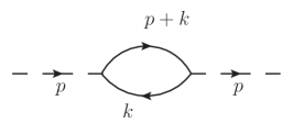
Figure 4: Self-energy loop graph in the scalar sector.

It is represented by the integral

$$i\Pi(p) = -\frac{g^{2}}{2}\phi(-p)\phi(p)\times$$ (32)

$$\times \int\frac{d^{4}k}{(2\pi)^{4}}\frac{{\rm Tr}\left((Q_{\mu}\gamma^{\mu}+m)(R_{\nu}\gamma^{\nu}+m)\right)}{(Q^{2}-m^{2})(R^{2}-m^{2})}\,,$$

where we define

$$Q_{\mu} = k_{\mu}-\bar{\alpha}mn_{\mu}-g_{2}n_{\mu}(n\cdot k)^{2}\,,$$

$$R_{\mu} = k_{\mu}+p_{\mu}-\bar{\alpha}mn_{\mu}-g_{2}n_{\mu}(n\cdot(k+p))^{2}\,.$$ (33)

Calculating the trace gives

$$i\Pi(p)=-2g^{2}\phi(-p)\phi(p)\int\frac{d^{4}k}{(2\pi)^{4}}\frac{Q\cdot R+m^{2}}{(Q^{2}-m^{2})(R^{2}-m^{2})}\,.$$

In principle, within our calculations, in the denominators $Q^{2}-m^{2}$ and $R^{2}-m^{2}$ we can suppress the terms proportional to $\bar{\alpha}$ since they yield only subleading orders. Let us write the corresponding contribution to the effective action as $i\Pi(p)=-2g^{2}\phi(-p)\widetilde{\Pi}(p)\phi(p)$ and study the typical low-energy behavior of this contribution by expanding it into Taylor series

$$\widetilde{\Pi}(p) = \widetilde{\Pi}(0)+p_{\mu}\left(\frac{\partial\widetilde{\Pi}}{\partial p_{\mu}}\right)_{p=0}+\frac{1}{2}p_{\mu}p_{\nu}\left(\frac{\partial^{2}\widetilde{\Pi}}{\partial p_{\mu}\partial p_{\nu}}\right)_{p=0}$$

$$+\dots\,.$$ (35)

The zeroth-order contribution follows directly from (5.1):

$$\widetilde{\Pi}(0)=\int\frac{d^{4}k}{(2\pi)^{4}}\frac{Q^{2}+m^{2}}{(Q^{2}-m^{2})^{2}}\,.$$ (36)

It is convenient to rewrite as

$$\widetilde{\Pi}(0)=K+2m^{2}P\,,$$ (37)

where

$$K=\int\frac{d^{4}k}{(2\pi)^{4}}\frac{1}{(Q^{2}-m^{2})}\,,$$ (38)

and

$$P=\int\frac{d^{4}k}{(2\pi)^{4}}\frac{1}{(Q^{2}-m^{2})^{2}}\,.$$ (39)

where the integrals (38) and (39) have been solved in the Appendix A.

For the next term, it is clear that $(\frac{\partial\widetilde{\Pi}}{\partial p^{\mu}})|_{p=0}$ can be proportional to $n_{\mu}$ only since there is no other vectors, the corresponding contribution to the effective action will yield
$\int d^{4}x\phi(n\cdot\partial)\phi$, that is, a surface term. So, we can disregard it. Further, one would need then to find the second derivative, that is, $(\frac{\partial^{2}\widetilde{\Pi}}{\partial p_{\mu}\partial p_{\nu}})|_{p=0}$ which may contain naturally terms of higher-order in $g_{2}$. To find it, consider

$$\left(\frac{\partial^{2}\widetilde{\Pi}(p)}{\partial p_{\mu}\partial p_{\nu}}\right)_{p=0} = \int\frac{d^{4}k}{(2\pi)^{4}}{\rm Tr}\Big{[}\left(\frac{1}{\not{Q}-m}\right)$$ (40)

$$\times \left[\frac{\partial}{\partial p_{\mu}}\frac{\partial}{\partial p_{\nu}}\left(\frac{1}{\not{R}-m}\right)\right]_{p=0}\Big{]}\,.$$

Integrating by parts and neglecting the surface terms, we obtain the symmetric expression

$$\left(\frac{\partial^{2}\widetilde{\Pi}(p)}{\partial p_{\mu}\partial p_{\nu}}\right)_{p=0} = -\int\frac{d^{4}k}{(2\pi)^{4}}{\rm Tr}\Big{[}\frac{\partial}{\partial k_{\nu}}\left(\frac{1}{\not{Q}-m}\right)$$ (41)

$$\times \frac{\partial}{\partial k_{\mu}}\left(\frac{1}{\not{Q}-m}\right)\Big{]}\,,$$

where we have used the identity $\left(\frac{\partial f(k+p)}{\partial p_{\alpha}}\right)_{p=0}=\frac{\partial f(k)}{\partial k_{\alpha}}$.

We consider

$$\frac{\partial}{\partial k_{\mu}}\left(\frac{1}{\not{Q}-m}\right)=\left(\frac{\partial Q_{\alpha}}{\partial k_{\mu}}\right)\frac{1}{(\not{Q}-m)^{2}}\gamma^{\alpha}\,,$$ (42)

and after some algebra we arrive at

$$\left(\frac{\partial^{2}\widetilde{\Pi}(p)}{\partial p_{\mu}\partial p_{\nu}}\right)_{p=0}=-\int\frac{d^{4}k}{(2\pi)^{4}}\left(\frac{\partial Q_{\alpha}}{\partial k_{\mu}}\right)\left(\frac{\partial Q_{\sigma}}{\partial k_{\nu}}\right)T^{\alpha\sigma}\,,$$ (43)

with

$$T^{\alpha\sigma}=\frac{4}{(Q^{2}-m^{2})^{2}}\eta^{\alpha\sigma}+\frac{32m^{2}}{(Q^{2}-m^{2})^{4}}Q^{\alpha}Q^{\sigma}\,.$$ (44)

By using the relations

$$\left(\frac{\partial Q_{\alpha}}{\partial k_{\mu}}\right)\left(\frac{\partial Q^{\alpha}}{\partial k_{\nu}}\right)=\eta^{\mu\nu}-4g_{2}n^{\mu}n^{\nu}(n\cdot Q)\,,$$

$$\left(\frac{\partial Q_{\alpha}}{\partial k_{\mu}}\right)\left(\frac{\partial Q_{\sigma}}{\partial k_{\nu}}\right)Q^{\alpha}Q^{\sigma}=\frac{1}{4}\left(\frac{\partial Q^{2}}{\partial k_{\mu}}\right)\left(\frac{\partial Q^{2}}{\partial k_{\nu}}\right)\,,$$ (45)

one obtains

$$\left(\frac{\partial^{2}\widetilde{\Pi}(p)}{\partial p_{\mu}\partial p_{\nu}}\right)_{p=0}=-4\int\frac{d^{4}k}{(2\pi)^{4}}\left(\frac{\eta^{\mu\nu}-4g_{2}n^{\mu}n^{\nu}(n\cdot Q)}{(Q^{2}-m^{2})^{2}}\right.$$

$$\left.+\frac{2m^{2}}{(Q^{2}-m^{2})^{4}}\left(\frac{\partial Q^{2}}{\partial k_{\mu}}\right)\left(\frac{\partial Q^{2}}{\partial k_{\nu}}\right)\right)\,.$$ (46)

Considering the tensors available in our model, which are the flat metric $\eta_{\mu\nu}$ and the preferred four-vector $n_{\mu}$ we can write

$$\int\frac{d^{4}k}{(2\pi)^{4}}\frac{Q_{\mu}}{(Q^{2}-m^{2})^{2}}=n_{\mu}S\,,$$ (47)

and

$$\int\frac{d^{4}k}{(2\pi)^{4}}\frac{1}{(Q^{2}-m^{2})^{4}}\left(\frac{\partial Q^{2}}{\partial k_{\mu}}\right)\left(\frac{\partial Q^{2}}{\partial k_{\nu}}\right)=$$ (48)

$$= n^{\mu}n^{\nu}L+\eta^{\mu\nu}n^{2}M\,.$$

Now, consider the relation

$$\frac{\partial Q^{2}}{\partial k_{\mu}}=2\left(Q^{\mu}-2g_{2}n^{\mu}(n\cdot Q)(n\cdot k)\right)\,,$$ (49)

and multiplying it by $n_{\mu}n_{\nu}$ we arrive at

$$\int\frac{d^{4}k}{(2\pi)^{4}}\frac{4(n\cdot Q)^{2}}{(Q^{2}-m^{2})^{4}}\left(1-4g_{2}n^{2}(n\cdot k)\right.$$ (50)

$$+ \left.4g_{2}^{2}(n^{2})^{2}(n\cdot k)^{2}\right)=(n^{2})^{2}(L+M)\,,$$

and by contracting with the metric $\eta_{\mu\nu}$

$$\int\frac{d^{4}k}{(2\pi)^{4}}\frac{4}{(Q^{2}-m^{2})^{4}}\left(Q^{2}-4g_{2}(n\cdot Q)^{2}(n\cdot k)\right.$$

$$\left.+4g_{2}^{2}n^{2}(n\cdot Q)^{2}(n\cdot k)^{2}\right)=n^{2}(L+4M)\,.$$ (51)

Solving the algebraic equation we have

$$L = \frac{16}{3n^{2}}\int\frac{d^{4}k}{(2\pi)^{4}}\frac{1}{(Q^{2}-m^{2})^{4}}\left(\frac{(n\cdot Q)^{2}}{n^{2}}-\frac{Q^{2}}{4}\right.$$

$$\left.-3g_{2}(n\cdot Q)^{2}(n\cdot k)+3g_{2}^{2}(n\cdot Q)^{2}(n\cdot k)^{2}n^{2}\right)\,,$$

$$M = \frac{4}{3n^{2}}\int\frac{d^{4}k}{(2\pi)^{4}}\frac{1}{(Q^{2}-m^{2})^{4}}\left(Q^{2}-\frac{(n\cdot Q)^{2}}{n^{2}}\right)\,.$$ (52)

A similar analysis gives

$$S=\frac{1}{n^{2}}\int\frac{d^{4}k}{(2\pi)^{4}}\frac{(n\cdot Q)}{(Q^{2}-m^{2})^{2}}\,.$$ (53)

We find the second-order contribution

$$\left(\frac{\partial^{2}\widetilde{\Pi}(p)}{\partial p_{\mu}\partial p_{\nu}}\right)_{p=0}p^{\mu}p^{\nu}=-\left(4P+8m^{2}n^{2}M\right)p^{2}$$

$$+\left(16g_{2}n^{2}S-8m^{2}L\right)(n\cdot p)^{2}\,.$$ (54)

Reorganizing this expression, we can write the correction to the scalar propagator up to second-order in $p$ as

$$\widetilde{\Pi}(p) = m^{2}q_{0}+p^{2}q_{1}+(n\cdot p)^{2}q_{n}\,,$$ (55)

where

$$q_{0} = \frac{K}{m^{2}}+2P\,,$$ (56)

$$q_{1} = -4\left(P+2m^{2}n^{2}M\right)\,,$$

$$q_{n} = 8\left(2g_{2}n^{2}S-m^{2}L\right)\,.$$

Finally one has

$$q_{0} = -\frac{i}{48\pi^{2}g_{2}^{2}m^{2}}+\frac{i}{16\pi^{2}}\left(2(3\gamma_{E}-1)-0.46\right.$$

$$\left.-3\ln\left(\frac{g_{2}^{2}m^{2}}{4}\right)\right)\,,$$

$$q_{1} = -\frac{i}{12\pi^{2}}\left(-5+6\gamma_{E}-0.46-3\ln\left(\frac{g_{2}^{2}m^{2}}{4}\right)\right)\,,$$ (58)

$$q_{n} = \frac{i}{\pi^{2}}\,.$$ (59)

We provide details of the computation of $q_{0}$, $q_{1}$ and $q_{n}$ in the Appendix A. The two-point function is finite and involves a fine-tuning term proportional to $g_{2}^{-2}$. The Lee-Wick modes improve the convergence of the theory such to make the two-point function of the scalar field essentially UV finite and involves the aether term ouraether .

5.2 Fermion self-energy ${\Sigma}(p)$

Now we focus on the contribution of the fermion self-energy graph depicted in Fig. 5, and recall that here we consider $M=m$.

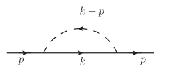
Figure 5: The fermion self-energy graph.

The fermion self-energy graph is represented by the integral

$$i{\Sigma}(p)=g^{2}\int\frac{d^{4}k}{(2\pi)^{4}}\frac{\not{Q}+m}{((k-p)^{2}-m^{2})(Q^{2}-m^{2})}\,.$$ (60)

To find it, let us consider a Taylor expansion of the first denominator term up to second-order in $p$ and rewrite this contribution as

$$i{\Sigma}(p)\approx g^{2}\int\frac{d^{4}k}{(2\pi)^{4}}\left(\frac{1}{k^{2}-m^{2}}+\frac{2(k\cdot p)-p^{2}}{(k^{2}-m^{2})^{2}}+\right.$$ (61)

$$+ \left.\frac{4(k\cdot p)^{2}}{(k^{2}-m^{2})^{3}}\right)\left(\frac{\not{Q}+m}{Q^{2}-m^{2}}\right)+\mathcal{O}(p^{3},n)\,.$$

With the notation $i{\Sigma}(p)=g^{2}I^{(0)}+g^{2}I^{(1)}+g^{2}I^{(2)}$, we introduce the the zeroth-order contribution

$$I^{(0)}=\int\frac{d^{4}k}{(2\pi)^{4}}\left(\frac{1}{k^{2}-m^{2}}\right)\left(\frac{\not{Q}+m}{Q^{2}-m^{2}}\right)\,,$$ (62)

the linear-order contribution

$$I^{(1)}=\int\frac{d^{4}k}{(2\pi)^{4}}\left(\frac{2(k\cdot p)}{(k^{2}-m^{2})^{2}}\right)\left(\frac{\not{Q}+m}{Q^{2}-m^{2}}\right)\,,$$ (63)

and the second-order contribution

$$I^{(2)} = \int\frac{d^{4}k}{(2\pi)^{4}}\left(\frac{4(k\cdot p)^{2}}{(k^{2}-m^{2})^{3}}-\frac{p^{2}}{(k^{2}-m^{2})^{2}}\right)\left(\frac{\not{Q}+m}{Q^{2}-m^{2}}\right)\,.$$

5.3 The gamma-matrix structure of $I^{(0)}$, $I^{(1)}$ $I^{(2)}$

5.3.1 Zeroth-order $I^{(0)}$

Let us start with Eq. (62) and rewrite it as

$$I^{(0)} = \gamma^{\mu}I_{\mu}^{(0)}+mf_{0}\,,$$ (65)

where we have defined

$$I_{\mu}^{(0)} = \int\frac{d^{4}k}{(2\pi)^{4}}\frac{Q_{\mu}}{(k^{2}-m^{2})(Q^{2}-m^{2})}\,,$$ (66)

and

$$f_{0} = \int\frac{d^{4}k}{(2\pi)^{4}}\frac{1}{(k^{2}-m^{2})(Q^{2}-m^{2})}\,.$$ (67)

From tensor analysis considerations one should have

$$\int\frac{d^{4}k}{(2\pi)^{4}}\frac{Q_{\mu}}{(k^{2}-m^{2})(Q^{2}-m^{2})}=n_{\mu}f_{1}^{n}\,.$$ (68)

Replacing the expression (68) in Eq. (65) produces the zeroth-order contribution

$$I^{(0)}=\not{n}f_{1}^{n}+mf_{0}\,,$$ (69)

with

$$f_{1}^{n} = \frac{1}{n^{2}}\int\frac{d^{4}k}{(2\pi)^{4}}\frac{(n\cdot Q)}{(k^{2}-m^{2})(Q^{2}-m^{2})}\,.$$ (70)

We carry out the calculations of $f_{0}$ and $f_{1}^{n}$ following the lines given in Appendix B.2. The first coefficient $f_{0}$ is naturally finite and the second one $f_{1}^{n}$ is divergent and contains a large Lorentz-breaking correction term of the order of $g_{2}^{-1}$.

5.3.2 Linear-order $I^{(1)}$

The linear-order integral (63) can be rewritten by introducing

$$I^{(1)}=2p^{\mu}\gamma^{\nu}I_{\mu\nu}^{(1)}+2mp^{\mu}I_{\mu}^{(1)}\,,$$ (71)

where

$$I_{\mu}^{(1)} = \int\frac{d^{4}k}{(2\pi)^{4}}\frac{k_{\mu}}{(k^{2}-m^{2})^{2}(Q^{2}-m^{2})}\,,$$ (72)

$$I_{\mu\nu}^{(1)} = \int\frac{d^{4}k}{(2\pi)^{4}}\frac{k_{\mu}Q_{\nu}}{(k^{2}-m^{2})^{2}(Q^{2}-m^{2})}\,.$$

By considering

$$\int\frac{d^{4}k}{(2\pi)^{4}}\frac{k_{\mu}}{(k^{2}-m^{2})^{2}(Q^{2}-m^{2})} = n_{\mu}D\,,$$ (73)

$$\int\frac{d^{4}k}{(2\pi)^{4}}\frac{k_{\mu}Q_{\nu}}{(k^{2}-m^{2})^{2}(Q^{2}-m^{2})} = n_{\mu}n_{\nu}B+n^{2}\eta_{\mu\nu}C\,,$$

and after some manipulations one finds

$$D=\frac{1}{n^{2}}\int\frac{d^{4}k}{(2\pi)^{4}}\frac{(n\cdot k)}{(k^{2}-m^{2})^{2}(Q^{2}-m^{2})}\,,$$ (74)

$$B=\frac{1}{3n^{2}}\int\frac{d^{4}k}{(2\pi)^{4}}\frac{\frac{4(n\cdot k)(n\cdot Q)}{n^{2}}-(k\cdot Q)}{(k^{2}-m^{2})^{2}(Q^{2}-m^{2})}\,,$$

$$C=\frac{1}{3n^{2}}\int\frac{d^{4}k}{(2\pi)^{4}}\frac{(k\cdot Q)-\frac{(n\cdot k)(n\cdot Q)}{n^{2}}}{(k^{2}-m^{2})^{2}(Q^{2}-m^{2})}\,.$$

Introducing the new notation we can write

$$I^{(1)}=\not{p}f_{1}+m(n\cdot p)f_{2}^{n}+\not{n}(n\cdot p)f_{3}^{n}\,,$$ (75)

where

$$f_{1} = 2n^{2}C\,,$$ (76)

$$f_{2}^{n} = 2D\,,$$ (77)

$$f_{3}^{n} = 2B\,.$$ (78)

The terms $f_{1}$, $f_{2}^{n}$ and $f_{3}^{n}$ are convergent and are explicitly calculated in Appendix B.3.

5.3.3 Second-order $I^{(2)}$

Following the same methodology the integral $I^{(2)}$ can be written as

$$I^{(2)} = -p^{2}\left(\gamma^{\mu}{{I}}_{\mu}^{(2)}+m{f_{2}}\right)+4p^{\mu}p^{\nu}\left(\gamma^{\alpha}{{I}}_{\mu\nu\alpha}^{(2)}+m{{I}}_{\mu\nu}^{(2)}\right)\,,$$ (79)

with

$${{I}}_{\mu}^{(2)} = \int\frac{d^{4}k}{(2\pi)^{4}}\frac{Q_{\mu}}{(k^{2}-m^{2})^{2}(Q^{2}-m^{2})}\,,$$

$${{I}}_{\mu\nu}^{(2)} = \int\frac{d^{4}k}{(2\pi)^{4}}\frac{k_{\mu}k_{\nu}}{(k^{2}-m^{2})^{3}(Q^{2}-m^{2})}\,,$$

$${{I}}_{\mu\nu\alpha}^{(2)} = \int\frac{d^{4}k}{(2\pi)^{4}}\frac{k_{\mu}k_{\nu}Q_{\alpha}}{(k^{2}-m^{2})^{3}(Q^{2}-m^{2})}\,,$$

$$f_{2} = \int\frac{d^{4}k}{(2\pi)^{4}}\frac{1}{(k^{2}-m^{2})^{2}(Q^{2}-m^{2})}\,.$$ (80)

We have that ${{I}}_{\mu\nu}^{(2)}$ and $f_{2}$ are of the order $g_{2}^{2}$ so they can be neglected. For the remaining we define them with the following tensor structure

$$\int\frac{d^{4}k}{(2\pi)^{4}}\frac{Q_{\mu}}{(k^{2}-m^{2})^{2}(Q^{2}-m^{2})} = n_{\mu}\bar{C}\,,$$ (81)

$$\int\frac{d^{4}k}{(2\pi)^{4}}\frac{k_{\mu}k_{\nu}Q_{\alpha}}{(k^{2}-m^{2})^{3}(Q^{2}-m^{2})}=n_{\mu}n_{\nu}n_{\alpha}\bar{D}$$ (82)

$$+n^{2}\eta_{\mu\nu}n_{\alpha}\bar{E}+n^{2}\eta_{\nu\alpha}n_{\mu}\bar{F}\,.$$

After some algebra we find

$$\bar{C} = \frac{1}{n^{2}}\int\frac{d^{4}k}{(2\pi)^{4}}\frac{(n\cdot Q)}{(k^{2}-m^{2})^{2}(Q^{2}-m^{2})},$$

$$\bar{E} = \frac{1}{3(n^{2})^{2}}\int\frac{d^{4}k}{(2\pi)^{4}}\frac{\left(k^{2}-\frac{(n\cdot k)^{2}}{n^{2}}\right)(n\cdot Q)}{(k^{2}-m^{2})^{3}(Q^{2}-m^{2})}\,,$$

$$\bar{D} = \frac{1}{3(n^{2})^{2}}\times$$

$$\times \int\frac{d^{4}k}{(2\pi)^{4}}\frac{\left(\frac{5(n\cdot k)^{2}(n\cdot Q)}{n^{2}}-k^{2}(n\cdot Q)-(n\cdot k)(k\cdot Q)\right)}{(k^{2}-m^{2})^{3}(Q^{2}-m^{2})},\,$$

$$\bar{F} = -\frac{1}{3(n^{2})^{2}}\int\frac{d^{4}k}{(2\pi)^{4}}\frac{\left(\frac{(n\cdot k)^{2}(n\cdot Q)}{n^{2}}-(n\cdot k)(k\cdot Q)\right)}{(k^{2}-m^{2})^{3}(Q^{2}-m^{2})}.\,$$ (83)

Replacing the expressions (5.3.3) in (79) and using the integrals (5.3.3), up to linear-order in Lorentz violation and second-order in $p$, we arrive at

$$I^{(2)} = p^{2}\not{n}(-\bar{C}+4n^{2}\bar{E})+4n^{2}(n\cdot p)\not{p}\bar{F}+4(n\cdot p)^{2}\not{n}\bar{D}\,.$$ (84)

We rewrite as

$$I^{(2)} = p^{2}\not{n}f_{6}^{n}+(n\cdot p)\not{p}f_{4}^{n}+(n\cdot p)^{2}\not{n}f_{5}^{n}\,,$$ (85)

with

$$f_{4}^{n} = 4n^{2}\bar{F}\,,$$ (86)

$$f_{5}^{n} = 4\bar{D}\,,$$ (87)

$$f_{6}^{n} = -\bar{C}+4n^{2}\bar{E}\,,$$ (88)

where the explicit form of the relevant constants is given in the Appendix B.4.

6 Mass renormalization

6.1 The on-shell subtraction scheme

Having computed the one-loop correction to the scalar and fermion propagators, we now proceed to determine the pole mass in our Yukawa-like model. The radiative corrections essentially involve extra terms such as the scalar $(n\cdot p)$, the matrix $\not{n}$ and their combinations. The theory is finite in the scalar sector and in the fermion sector the only divergency appears in the term $f_{1}^{n}$. Since the mass corrections are finite in both sectors, in some sense we are working in the scheme in which the finite parts of the renormalized mass correspond to the pole mass, and hence one can say that we are working in the on-shell subtraction scheme. Most of the ideas and method of calculation in the derivation of the pole mass, which are given below, are along the lines developed in the work of Ref. ralf .

Let us remind the leading quantum corrections in the scalar sector

$$i\Pi(p) = -2g^{2}m^{2}q_{0}-2g^{2}p^{2}q_{1}-2g^{2}(n\cdot p)^{2}q_{n}\,,$$ (89)

where we have restored the constant $-2g^{2}$. In the fermion sector we have found

$$i\Sigma_{2} = g^{2}\not{n}f_{1}^{n}+g^{2}mf_{0}+g^{2}\not{p}f_{1}+g^{2}m(n\cdot p)f_{2}^{n}+g^{2}\not{n}(n\cdot p)f_{3}^{n}$$ (90)

$$+g^{2}p^{2}\not{n}f_{6}^{n}+g^{2}(n\cdot p)\not{p}f_{4}^{n}+g^{2}(n\cdot p)^{2}\not{n}f_{5}^{n}\,.$$

The coefficients $q$ and $f$ have been computed in the Appendices A and B.

6.2 The scalar pole mass

Let us start with the finite scalar Lagrangian

$${\cal L}_{\phi} = \frac{1}{2}\partial_{\mu}\phi\partial^{\mu}\phi-\frac{1}{2}M^{2}\phi^{2}\,,$$ (91)

in which no counterterms are needed to control ultraviolet divergencies. The renormalized scalar two-point function is given by

$$(\Gamma_{\phi,R}^{(2)})^{-1}=p^{2}-M^{2}+\Pi_{R}(p)\,,$$ (92)

where

$$\Pi_{R}(p)=p^{2}A_{\phi}+m^{2}B_{\phi}+(n\cdot p)^{2}C_{\phi}\,,$$ (93)

where $A_{\phi}$, $B_{\phi}$ and $C_{\phi}$ are constants that can be deduced from the expressions (5.1), (58), (59) being

$$iA_{\phi} = -2g^{2}q_{1}\,,$$

$$iB_{\phi} = -2g^{2}q_{0}\,,$$

$$iC_{\phi} = -2g^{2}q_{n}\,.$$ (94)

We define

$$\bar{P}^{2}_{\phi}=p^{2}-{M}^{2}_{{\rm ph}}+\bar{y}(n\cdot p)^{2}\,.$$ (95)

in terms of the two unknown constants $M_{{\rm ph}}$ and $\bar{y}$, Both constants can be determine with the renormalization condition at $\bar{P}^{2}_{\phi}=0$

$$(\Gamma_{\phi,R}^{(2)})^{-1}(\bar{P}_{\phi}^{2}=0)=0\,.$$ (96)

Hence, from (92) replacing the value of $p^{2}$ given in (95) and using the condition (96), we arrive at the equation

$$0 = {M}^{2}_{{\rm ph}}-\bar{y}(n\cdot p)^{2}-M^{2}+A_{\phi}\left({M}^{2}_{{\rm ph}}-\bar{y}(n\cdot p)^{2}\right)$$ (97)

$$+ B_{\phi}m^{2}+C_{\phi}(n\cdot p)^{2}\,.$$

Due to the independence of each term, we find the two constants

$${M}^{2}_{{\rm ph}}=\frac{(M^{2}-B_{\phi}m^{2})}{(1+A_{\phi})}\,,\qquad\bar{y}=\frac{C_{\phi}}{1+A_{\phi}}\,,$$ (98)

and in consequence also the scalar pole mass $\bar{P}_{\phi}^{2}$. Substituting the above expressions in Eq. (92) and using

$$\frac{(\Gamma_{\phi,R}^{(2)})^{-1}(0)}{d\bar{P}^{2}_{\phi}}=Z_{\phi}^{-1}\,,$$ (99)

we identify the wave function normalization $Z_{\phi}^{-1}=1+A_{\phi}$, which in this case is finite.

6.3 The fermion pole mass

The fermionic Lagrangian written in terms of renormalized quantities reads

$${\cal L}_{\psi} = i\bar{\psi}\partial\!\!\!/\psi-m\bar{\psi}\psi-\bar{\alpha}_{R}m\bar{\psi}n\!\!\!/\psi+g_{2}\bar{\psi}\not{n}(n\cdot\partial)^{2}\psi$$ (100)

$$- \delta_{\bar{\alpha}}\bar{\alpha}_{R}m\bar{\psi}\not{n}\psi\,,$$

where $\bar{\alpha}=Z_{\bar{\alpha}}\bar{\alpha}_{R}$ and $Z_{\bar{\alpha}}=1+\delta_{\bar{\alpha}}$ and all other $Z_{X}$ equal to one. The renormalized fermion two-point function is

$$(\Gamma_{\psi,R}^{(2)})^{-1}=\not{p}-m+\Sigma_{R}\,,$$ (101)

with

$$\Sigma_{R}=\Sigma_{2}-\delta_{\bar{\alpha}}\bar{\alpha}_{R}m\not{n}+\mathcal{O}(g^{4})\,.$$ (102)

We can write the finite contribution to the renormalized two-point function up to second-order in $p$ as

$$\Sigma_{R}=\not{p}A_{\psi}+mB_{\psi}+\not{n}C_{\psi}\,,$$ (103)

where the explicit Lorentz violation coefficients at linear order in $g_{2}$, and coded in $\Sigma_{2}$, are given by

$$A_{\psi} = A^{(0)}+g_{2}A^{(1)}(n\cdot p)\,,$$

$$B_{\psi} = B^{(0)}+g_{2}B^{(1)}(n\cdot p)\,,$$

$$C_{\psi} = \frac{C^{(0)}}{g_{2}}+C^{(1)}(n\cdot p)+g_{2}C^{(2)}(n\cdot p)^{2}+g_{2}C^{(3)}p^{2}\,.$$ (104)

We work in the minimal subtraction scheme and hence we fix the divergent term to be

$$\delta_{\bar{\alpha}}=\frac{g^{2}}{4\bar{\alpha}_{R}g_{2}m\pi^{2}\epsilon}\,,$$ (105)

in accordance with the correction term in (170). Within this scheme and according to the previous calculations we make the identification

$$iA^{(0)}=g^{2}f_{1}\,,\qquad iA^{(1)}=\frac{g^{2}f_{4}^{n}}{g_{2}}\,,\qquad iB^{(0)}=g^{2}f_{0}\,,$$

$$iB^{(1)}=\frac{g^{2}f_{2}^{n}}{g_{2}}\,,\qquad iC^{(0)}=g_{2}(g^{2}f_{1}^{n}-\delta_{\bar{\alpha}}\bar{\alpha}_{R})\,,$$

$$iC^{(1)}=g^{2}f_{3}^{n}\,,\qquad iC^{(2)}=\frac{g^{2}f_{5}^{n}}{g_{2}}\,,\qquad iC^{(3)}=\frac{g^{2}f_{6}^{n}}{g_{2}}\,.$$ (106)

To find the pole we consider the ansatz

$$\bar{P}=\not{p}-\bar{m}+\bar{x}\not{n}\,,$$ (107)

where

$$\bar{m}=m_{{\rm ph}}+g_{2}m_{n}(n\cdot p)\,,$$ (108)

and

$$\bar{x}=\frac{\bar{x}^{(0)}}{g_{2}}+\bar{x}^{(1)}(n\cdot p)+g_{2}\bar{x}^{(2)}(n\cdot p)^{2}+g_{2}\bar{x}^{(3)}p^{2}\,.$$ (109)

We include the large Lorentz violating terms in the pole extraction process which has been included explicitly in $\bar{x}$.

Considering the condition for $\bar{P}$ to be a pole, that is to say,

$$(\Gamma_{\psi,R}^{(2)})^{-1}(\bar{P}=0)=\not{p}-m+\Sigma_{R}=0\,,$$ (110)

provides us with the six terms $m_{ph}$, $m_{n}$, $\bar{x}^{(0)}$, $\bar{x}^{(1)}$, $\bar{x}^{(2)}$, $\bar{x}^{(3)}$. We proceed as follows: we replace $\bar{P}$ in (101), and arrive at

$$(\Gamma_{\psi,R}^{(2)})^{-1} = \bar{P}+\bar{m}-\bar{x}\not{n}-m+A(\bar{P}+\bar{m}-\bar{x}\not{n})+Bm+C\not{n}\,.$$

With $\bar{P}=0$ we write

$$(\Gamma_{\psi,R}^{(2)})^{-1}(\bar{P}=0)=0=m_{{\rm ph}}+g_{2}m_{n}(n\cdot p)-\bar{x}\not{n}-m$$ (112)

$$+ \Big{(}A^{(0)}+gA^{(1)}(n\cdot p)\Big{)}\Big{(}m_{{\rm ph}}+gm_{n}(n\cdot p)-\bar{x}\not{n}\Big{)}$$

$$+ \left(B^{(0)}+g_{2}B^{(1)}(n\cdot p)\right)m+\left(\frac{1}{g_{2}}C^{(0)}+C^{(1)}(n\cdot p)\right.$$

$$\left.+g_{2}C^{(2)}(n\cdot p)^{2}+g_{2}C^{(3)}p^{2}\right)\not{n}\,.$$

At lowest-order we have the first condition

$$m_{{\rm ph}}-m+A^{(0)}m_{ph}+B^{(0)}m=0\,,$$ (113)

which has the solution

$$m_{{\rm ph}}=m\frac{(1-B^{(0)})}{(1+A^{(0)})}\,.$$ (114)

Considering that all coefficients are independent, we have at linear-order for the factor accompanying $(n\cdot p)$:

$$g_{2}(n\cdot p)\left[m_{n}+A^{(0)}m_{n}+A^{(1)}m_{{\rm ph}}+B^{(1)}m\right]=0\,,$$

and consequently we have

$$m_{n}=-m\left(\frac{(A^{(1)}(1-B^{(0)})}{(1+A^{(0)})^{2}}+\frac{B^{(1)}}{1+A^{(0)}}\right)\,.$$ (116)

The next conditions determine $\bar{x}$ which follows from the equations with factor accompanying $\frac{1}{g_{2}}\not{n}$, $(n\cdot p)\not{n}$ , $g_{2}(n\cdot p)^{2}\not{n}$, $g_{2}p^{2}\not{n}$ respectively. Therefore, one arrives at

$$\bar{x}^{(0)} = \frac{C^{(0)}}{1+A^{(0)}}\,,$$

$$\bar{x}^{(1)} = -\frac{A^{(1)}C^{(0)}}{(1+A^{(0)})^{2}}+\frac{C^{(1)}}{1+A^{(0)}}\,,$$

$$\bar{x}^{(2)} = \frac{(A^{(1)})^{2}C^{(0)}}{(1+A^{(0)})^{3}}-\frac{A^{(1)}C^{(1)}}{(1+A^{(0)})^{2}}+\frac{C^{(2)}}{1+A^{(0)}}\,,$$

$$\bar{x}^{(3)} = \frac{C^{(3)}}{1+A^{(0)}}\,.$$ (117)

This finishes the pole extraction in both sectors.

Let us perform an analysis of renormalization group equations and consider the beta function for the renormalized parameter $\bar{\alpha}_{R}$

$$\beta(\bar{\alpha}_{R})=\mu\frac{d}{d\mu}\bar{\alpha}_{R}\,.$$ (118)

Recall, in our theory the $\bar{\alpha}$ parameter is renormalized through the relation

$$\bar{\alpha}=\bar{\alpha}_{R}\left(1+\frac{g^{2}}{4\bar{\alpha}_{R}g_{2}m\pi^{2}\epsilon}\right)\,,$$ (119)

where in terms of the bare coupling $g_{0}$ one has in $d$ dimension $g_{0}=\mu^{\epsilon/2}g$. From the condition

$$\mu\frac{d}{d\mu}\bar{\alpha}=0\,,$$ (120)

we find at leading order

$$\beta(\bar{\alpha}_{R})=\frac{g^{2}}{4g_{2}m\pi^{2}}\,.$$ (121)

We use the renormalization group equation

$$\frac{d\bar{\alpha}_{R}}{dt}=\beta(\bar{\alpha}_{R})\,,$$ (122)

which can be integrated as

$$\bar{\alpha}_{R}(t)=\bar{\alpha}_{R}(0)+\frac{g^{2}}{4g_{2}m\pi^{2}}t.$$ (123)

Hence we have no problems for low-energy domain but we can meet zero charge problem (Landau pole) at high energies for $g_{2}<0$.

7 Summary

We considered the Myers-Pospelov-like higher-derivative extensions of the Yukawa model which incorporates possible new physics from the Planck scale through dimension five operators coupled to a preferred four vector $n^{\mu}$ which breaks the Lorentz symmetry. We have selected a particular configuration of Lorentz symmetry violation in which the preferred four-vector $n^{\mu}$ is purely timelike. This choice produces higher-order time-derivative terms and leads to extra solutions and new poles in the model. We have found and identified the poles associated to standard solutions and those ones corresponding to negative-metric states or Lee-Wick solutions. Some of these poles move in the real axis, as in the usual Yukawa model. However, above a specific energy called the critical energy some solutions become complex introducing a extra difficulty for defining the consistent prescription for the contour of integration in the complex plane Anselmi2 . To solve this problem we have analyzed the motion of the poles in the complex plane. In the scalar sector we have defined the usual Feynman integration contour which rounds the negative pole from below and the positive from above; the new poles that appear are located in the imaginary axis and hence they do not present problems in this sense. However, in the fermion sector we have defined the prescription with two considerations in mind: first, the ability to recover the standard location of the poles relative to the real axis when the Lorentz invariance violation is turned off. With this consideration we have imposed the minimal requirement on the contour $C_{F}^{(f)}$ to round the negative pole $\omega_{2}$ from below and $\omega_{1}$ from above. Second, to account for the other poles we have used the prescription putted forward in QEDunitarity , which has been shown to lead to a unitary $S$-matrix in the regime of real solutions. Using this Lee-Wick prescription, the three positive solutions $W_{1}$, $W_{2}$ and $\omega_{1}$ are defined to lie below the contour and the negative one $\omega_{2}$ above. At higher energies beyond the critical energy, we have called for the following heuristic construction. We start at lower energies in which all the poles are real and where the basic requirements for consistency of the theory are satisfied. Next, we begin to increase the energy at which complex solutions appear and define the new contour as the one obtained by continuously deforming the first one in such a way to avoid any crossing and singularity with the complex poles.

A central part of this work has been the study of mass renormalization in the presence of both Lorentz-invariance violation and higher-order operators. We have computed the one-loop corrections in the model and shown how they lead to modifications in the renormalization procedure by pushing the pole mass to a sector involving other gamma matrices besides of $\not{p}$. The significance of our results, in particular, is based on the fact that this is one of the first works on the renormalization of higher-derivative Lorentz-breaking theories within the context of modifications of asymptotic Hilbert space, whereas even without introducing the higher derivatives the renormalization issues in Lorentz-breaking theory were considered only in a few papers, in particular One-loop ; scarp ; ba . For other approaches in renormalization of higher-order Lorentz breaking theories, see Anselmi1 . We found that the theory is super-renormalizable (in principle, increasing the value of $N$ in the added kinetic operator $(n\cdot\partial)^{N}$, we can get a completely finite theory, the same result can be achieved through a supersymmetric extension of the theory, see CMP ). The kinetic terms of the both fields are explicitly finite. As a by-product, we conclude that the aether-like terms originally introduced in ouraether ; class are generated within our studies both in scalar and spinor sectors, and they are essentially finite. It is interesting to note that in the spinor sector, the aether terms dominate in the low-energy limit in comparison with the second-derivative term we introduced into the classical action.

At the same time, the large quantum corrections or, in other words, fine-tuning arise in our theory. We have found in the scalar sector a large correction which in principle should be added to the usual fine tuning proportional to the square of the fermion mass. In consequence the effect of UV sensitivity of the scalar mass is maintained in our model. In the fermion sector we have that the large corrections affect a term which do not involve any physical observable protecting the theory in this sector to a genuine fine tuning. Actually, in our theory we have only one nontrivial counterterm, in the quadratic acton of the spinor. In a certain sense, this effect of large quantum corrections taking place in our theory resembles the effect of UV/IR mixing taking place in noncommutative field theories responsible for arising infrared singularities in a small noncommutativity limit Minw . Let us mention that in principle these large corrections are natural to expect since the higher-derivative extensions of the classical action can be treated as a kind of the higher-derivative regularization, hence, removing the regularization we return to singular results. We note that this effect is rather generic since the large quantum corrections are present even in the supersymmetric extensions of the Myers-Pospelov-like theories CMP . The complete elimination of large quantum corrections could consist in employing the extended supersymmetry which is well known to achieve complete finiteness of the field theory models as occurs for example for ${\cal N}=4$ super-Yang-Mills theory. Therefore, the natural problem could consist in study of some Myers-Pospelov-like extensions of ${\cal N}=4$ super-Yang-Mills theories. Another relevant problem consists in studying of the two-loop approximation thus exhausting the possible divergences. We plan to carry out these studies in one of our next papers.

Appendix A The calculation of $q_{0}$, $q_{1}$, $q_{n}$

We start to compute $q_{0}$ in (56), so we focus on $K$ and $P$ as given in Eqs. (38) and (39) and promote the integrals to $d$ dimensions and consider

$$d^{d}k = \Omega_{d-1}|{\vec{k}}|^{d-2}d|{\vec{k}}|\,dk_{0}$$ (124)

$$= \Omega_{d-1}E(E^{2}-m^{2})^{\frac{d-3}{2}}dE\,dk_{0}\,,$$

where we have performed an integration in the angles producing the solid angle in $d-1$ dimensions

$$\Omega_{d-1}=\frac{2\pi^{(d-1)/2}}{\Gamma\left(\frac{d-1}{2}\right)}\,.$$ (125)

From Eqs. (38) and (39), we note that

$$\frac{\partial K}{\partial m^{2}}=P\,.$$ (126)

So we first compute $K$ and then derive $P$. To compute $K$ we consider the integral

$$K = \mu^{4-d}\Omega_{d-1}\int_{m}^{\infty}\frac{E(E^{2}-m^{2})^{\frac{d-3}{2}}dE}{(2\pi)^{d}}$$ (127)

$$\times \int_{C_{F}^{(f)}}\frac{dk_{0}}{(Q^{2}-m^{2})}\,.$$

We rewrite the contour integrals making explicit their poles, and to compute them we use the method of residues and close the contour $C_{F}^{(f)}$ in the upper half plane as shown in Fig. 2. We find

$$\int_{C_{F}^{(f)}}\frac{dk_{0}}{g_{2}^{2}(k_{0}-\omega_{1})(k_{0}-\omega_{2})(k_{0}-W_{1})(k_{0}-W_{2})}$$ (128)

$$= -\frac{\pi i}{E\sqrt{1+4g_{2}E}}\,,$$

The next integral in the variable $E$ is direct, and gives at lowest order in $\epsilon=4-d$ the contribution

$$K = -\frac{i}{48\pi^{2}g_{2}^{2}}+\frac{im^{2}}{48\pi^{2}}\left(6\gamma_{E}-0.46\right.$$ (129)

$$- \left.3\ln\left(\frac{g_{2}^{2}m^{2}}{4}\right)\right)\,.$$

From the relation 126 one has

$$P = -\frac{i}{16\pi^{2}}+\frac{i}{48\pi^{2}}\left(6\gamma_{E}-0.46-3\ln\left(\frac{g_{2}^{2}m^{2}}{4}\right)\right)\,.$$ (130)

It is simple to show that by combining the two contributions through $q_{0}=K/m^{2}+2P$, produces

$$q_{0} = -\frac{i}{48\pi^{2}g_{2}^{2}m^{2}}+\frac{i}{16\pi^{2}}\left(2(3\gamma_{E}-1)-0.46\right.$$ (131)

$$\left.-3\ln\left(\frac{g_{2}^{2}m^{2}}{4}\right)\right)\,.$$

The second-order contributions $q_{1}$ and $q_{n}$ are given in terms of $P$, $M$, $S$ and $L$ as shown in Eqs. (56). We begin with $M$, and since it is obtainable in four dimension, we just set $d=4$, giving

$$M=-\frac{16\pi}{3}\int_{m}^{\infty}\frac{E(E^{2}-m^{2})^{3/2}dE}{(2\pi)^{4}}\int_{C_{F}^{(f)}}\frac{dk_{0}}{(Q^{2}-m^{2})^{4}}\,.$$ (132)

Solving the first integral gives

$$\int_{C_{F}^{(f)}}\frac{dk_{0}}{g_{2}^{8}(k_{0}-\omega_{1})^{4}(k_{0}-\omega_{2})^{4}(k_{0}-W_{1})^{4}(k_{0}-W_{2})^{4}}$$ (133)

$$= \frac{\pi i\left(5+2g_{2}E\left(35+4g_{2}E\left(43+77g_{2}E\right)\right)\right)}{16E^{7}(1+4g_{2}E)^{7/2}}\,,$$

and calculating then the $E$-integral, we arrive at

$$M = -\frac{i}{48\pi^{2}m^{2}}\,.$$ (134)

With the result of $P$ given in (130), one has

$$q_{1} = -\frac{i}{12\pi^{2}}\left(-5+6\gamma_{E}-0.46-3\ln\left(\frac{g_{2}^{2}m^{2}}{4}\right)\right)\,.$$ (135)

We continue to compute $q_{n}$. From (53) we have

$$S = \mu^{4-d}\Omega_{d-1}\int_{m}^{\infty}\frac{E(E^{2}-m^{2})^{(d-3)/2}dE}{(2\pi)^{d}}$$

$$\times \int_{C_{F}^{(f)}}\frac{k_{0}(1-g_{2}k_{0})\;dk_{0}}{g_{2}^{4}(k_{0}-\omega_{1})^{2}(k_{0}-\omega_{2})^{2}(k_{0}-W_{1})^{2}(k_{0}-W_{2})^{2}}\,.$$

In the same way, we arrive at

$$S=\frac{i}{16g_{2}\pi^{2}}+\frac{ig_{2}m^{2}}{16\pi^{2}}\left(-4+\gamma_{E}-0.15-2\ln\left(\frac{g_{2}m}{2}\right)\right)\,.$$

To compute $L$ given in the first equation (5.1),

$$L = \frac{16}{3n^{2}}\int\frac{d^{4}k}{(2\pi)^{4}}\frac{1}{(Q^{2}-m^{2})^{4}}\left(\frac{(n\cdot Q)^{2}}{n^{2}}-\frac{Q^{2}}{4}\right.$$ (138)

$$\left.-3g_{2}(n\cdot Q)^{2}(n\cdot k)+3g_{2}^{2}(n\cdot Q)^{2}(n\cdot k)^{2}n^{2}\right)\,,$$

we note that

$$L = L_{2}-M\,,$$ (139)

with

$$L_{2} = 16\pi\int_{m}^{\infty}\frac{E(E^{2}-m^{2})^{1/2}dE}{(2\pi)^{4}}$$

$$\times \int_{C_{F}^{(f)}}\frac{k_{0}^{2}(1-g_{2}k_{0})^{2}(1-2g_{2}k_{0})^{2}\;dk_{0}}{g_{2}^{8}(k_{0}-\omega_{1})^{4}(k_{0}-\omega_{2})^{4}(k_{0}-W_{1})^{4}(k_{0}-W_{2})^{4}}\,.$$

We find

$$L_{2} = -\frac{i}{48\pi^{2}m^{2}}\,,$$ (141)

and therefore $L=0$. Considering the leading contributions for $q_{n}$ we obtain

$$q_{n} = \frac{i}{\pi^{2}}\,.$$ (142)

Appendix B The calculation of $\Sigma(p)$

B.1 The general strategy

In this subsection, we describe the main steps to derive the basic integral that will appear in the computation of the fermion self-energy correction (61). Let us start to consider the integral below where each order is labelled with $\alpha=1,2,3$

$$M_{(\alpha)}=\int\frac{d^{4}k}{(2\pi)^{4}}\frac{F(k_{0},\vec{k})}{(k^{2}-m^{2})^{\alpha}(Q^{2}-m^{2})}\,,$$ (143)

and where $F(k_{0},\vec{k})$ is an arbitrary function of $k_{0}$ and $\vec{k}$.

We promote the integrals to $d$ dimensions and recall the phase space measure given in (124) in order to write

$$M_{(\alpha)} = \mu^{4-d}\Omega_{d-1}\int_{m}^{\infty}\frac{dE}{(2\pi)^{d}}E(E^{2}-m^{2})^{\frac{d-3}{2}}$$ (144)

$$\times \int_{C_{F}^{(f)}}\frac{F(k_{0},\vec{k})\;dk_{0}}{(k_{0}^{2}-E^{2})^{\alpha}((k_{0}-\bar{\alpha}m-g_{2}k_{0}^{2})^{2}-E^{2})}\,.$$

To simplify the calculation, we will in the sequel everywhere approximate $(k_{0}-\bar{\alpha}m-g_{2}k_{0}^{2})^{2}-E^{2})\simeq(k_{0}-g_{2}k_{0}^{2})^{2}-E^{2})$ in all denominators, which will have very small modifications of the result since, first, $\bar{\alpha}$ is very small, second, it contributes only to subleading orders of results. Working the denominator, we can rewrite the last contour integral as

$$-\frac{1}{2Eg_{2}}\int_{C_{F}^{(f)}}dk_{0}F(k_{0},\vec{k})\frac{1}{(k_{0}^{2}-E^{2})^{\alpha}}$$ (145)

$$\times \left(\frac{1}{\left(\frac{k_{0}(-1+g_{2}k_{0})+E}{g_{2}}\right)}-\frac{1}{\left(\frac{k_{0}(-1+g_{2}k_{0})-E}{g_{2}}\right)}\right)\,.$$

Now, using the Feynman parametrization

$$\frac{1}{A^{\alpha}B^{\beta}}=\frac{\Gamma({\alpha}+\beta)}{\Gamma({\alpha})\Gamma(\beta)}\int_{0}^{1}dx\frac{x^{{\alpha}-1}\left(1-x\right)^{\beta-1}}{\left(Ax+B\left(1-x\right)\right)^{{\alpha}+\beta}}\,,$$ (146)

and using $\beta=1$ we write the integral as

$$-\frac{\alpha}{2Eg_{2}}\int_{C_{F}^{(f)}}dk_{0}F(k_{0},\vec{k})\int_{0}^{1}dx$$ (147)

$$\times \left[\frac{x^{\alpha-1}}{\left[k_{0}^{2}-\frac{k_{0}(1-x)}{g_{2}}-E^{2}x+\frac{E(1-x)}{g_{2}}\right]^{\alpha+1}}\right.$$

$$\left.-\frac{x^{\alpha-1}}{\left[k_{0}^{2}-\frac{k_{0}(1-x)}{g_{2}}-E^{2}x-\frac{E(1-x)}{g_{2}}\right]^{\alpha+1}}\right]\,.$$

Next, we carry out the change of variables $k_{0}^{\prime}=k_{0}-\frac{(1-x)}{2g_{2}}$ and perform a subsequent Wick rotation $k_{0}^{\prime}\to ik_{0E}^{\prime}$, as a result, and dropping the tilde, we arrive at

$$\frac{i(-1)^{\alpha}\alpha}{2Eg_{2}}\int_{0}^{1}dx\int_{-\infty}^{\infty}dk_{0E}F\left(ik_{0E}+\frac{(1-x)}{2g_{2}},\vec{k}\right)$$ (148)

$$\times \left[\frac{x^{\alpha-1}}{\left[k_{0E}^{2}+E^{2}x-\frac{E(1-x)}{g_{2}}+\frac{(1-x)^{2}}{4g_{2}^{2}}\right]^{\alpha+1}}\right.$$

$$\left.-\frac{x^{\alpha-1}}{\left[k_{0E}^{2}+E^{2}x+\frac{E(1-x)}{g_{2}}+\frac{(1-x)^{2}}{4g_{2}^{2}}\right]^{\alpha+1}}\right]\,.$$

Replacing the above expression in (144) and again changing variables by the rule $t=g_{2}E$ produces the final expression

$$M_{(\alpha)} = \frac{i(-1)^{\alpha}\alpha\Omega_{d-1}\mu^{4-d}}{2}$$ (149)

$$\times \int_{g_{2}m}^{\infty}\frac{dt}{(2\pi)^{d}}\frac{1}{g_{2}^{d-1}}(t^{2}-g_{2}^{2}m^{2})^{\frac{(d-3)}{2}}l_{(\alpha)}\,,$$

with

$$l_{(\alpha)} = \int_{-\infty}^{\infty}dk_{0E}\int_{0}^{1}dxF\left(ik_{0E}+\frac{(1-x)}{2g_{2}},\vec{k}\right)$$ (150)

$$\times \left[\frac{x^{\alpha-1}}{\left[k_{0E}^{2}+\frac{t^{2}}{g_{2}^{2}}x-\frac{t(1-x)}{g_{2}^{2}}+\frac{(1-x)^{2}}{4g_{2}^{2}}\right]^{\alpha+1}}\right.$$

$$- \left.\frac{x^{\alpha-1}}{\left[k_{0E}^{2}+\frac{t^{2}}{g_{2}^{2}}x+\frac{t(1-x)}{g_{2}^{2}}+\frac{(1-x)^{2}}{4g_{2}^{2}}\right]^{\alpha+1}}\right]\,,$$

which is the basic integral we need to solve in the next subsections.

B.2 The zeroth-order terms $f_{0}$ and $f_{1}^{n}$

We start to compute $f_{0}$ in $d$ dimensions which follows from (67)

$$f_{0}=\mu^{4-d}\int\frac{d^{d}k}{(2\pi)^{d}}\frac{1}{(k^{2}-m^{2})(Q^{2}-m^{2})}\,.$$ (151)

We use the Eqs. (149) and (150) with the identification $\alpha=1$ and $F(k_{0},\vec{k})=1$, which yield

$$f_{0}=-\frac{i\Omega_{d-1}\mu^{4-d}}{2}\int_{g_{2}m}^{\infty}\frac{dt}{(2\pi)^{d}}\frac{1}{g_{2}^{d-1}}(t^{2}-g_{2}^{2}m^{2})^{\frac{(d-3)}{2}}l^{(1)}_{1}\,,$$

with

$$l_{1}^{(1)} = \int_{-\infty}^{\infty}dk_{0E}\int_{0}^{1}dx\left[\frac{1}{\left[k_{0E}^{2}+\frac{t^{2}}{g_{2}^{2}}x-\frac{t(1-x)}{g_{2}^{2}}+\frac{(1-x)^{2}}{4g_{2}^{2}}\right]^{2}}\right.$$ (153)

$$\left.-\frac{1}{\left[k_{0E}^{2}+\frac{t^{2}}{g_{2}^{2}}x+\frac{t(1-x)}{g_{2}^{2}}+\frac{(1-x)^{2}}{4g_{2}^{2}}\right]^{2}}\right]\,.$$

To proceed, we consider some useful integrals

$$\int_{-\infty}^{\infty}dk_{0E}\frac{1}{(k_{0E}^{2}+M^{2})^{r}}=\frac{\sqrt{\pi}}{\Gamma(r)}\frac{\Gamma(r-\frac{1}{2})}{(M^{2})^{r-\frac{1}{2}}}\,,$$ (154)

$$\int_{-\infty}^{\infty}dk_{0E}\frac{k_{0E}^{2}}{(k^{2}_{0E}+M^{2})^{r}}=\frac{\sqrt{\pi}}{2\Gamma(r)}\frac{\Gamma(r-\frac{3}{2})}{(M^{2})^{r-\frac{3}{2}}}\,,$$ (155)

$$\int_{-\infty}^{\infty}dk_{0E}\frac{k_{0E}^{4}}{(k^{2}_{0E}+M^{2})^{r}}=\frac{3\sqrt{\pi}}{4\Gamma(r)}\frac{\Gamma(r-\frac{5}{2})}{(M^{2})^{r-\frac{5}{2}}}\,.$$ (156)

By using the integral (154) for $r=2$, we are able to solve the time integral in (153) arriving at

$$l_{1}^{(1)} = \frac{\pi}{2}\int_{0}^{1}dx\left[\frac{1}{(\frac{t^{2}}{g_{2}^{2}}x-\frac{t(1-x)}{g_{2}^{2}}+\frac{(1-x)^{2}}{4g_{2}^{2}})^{3/2}}\right.$$ (157)

$$\left.-\frac{1}{(\frac{t^{2}}{g_{2}^{2}}x+\frac{t(1-x)}{g_{2}^{2}}+\frac{(1-x)^{2}}{4g_{2}^{2}})^{3/2}}\right].$$

Introducing the new variable $\varepsilon=t(1-x)$, we write

$$l_{1}^{(1)} = \frac{g_{2}^{3}\pi}{2}\int_{0}^{1}dx\left[\frac{1}{(t^{2}x-\varepsilon+\frac{(1-x)^{2}}{4})^{3/2}}\right.$$ (158)

$$\left.-\frac{1}{(t^{2}x+\varepsilon+\frac{(1-x)^{2}}{4})^{3/2}}\right]\,.$$

We use the approximation

$$\frac{1}{(t^{2}x-\varepsilon+\frac{(1-x)^{2}}{4})^{n/2}}-\frac{1}{(t^{2}x+\varepsilon+\frac{(1-x)^{2}}{4})^{n/2}}$$ (159)

$$= \frac{n\varepsilon}{(t^{2}x+\frac{(1-x)^{2}}{4})^{n/2+1}}+\mathcal{O}(\varepsilon^{3})\,,$$

for $n=3$ followed by replacing $d=4$ in all explicitly finite terms, as a result, we arrive at the expression

$$f_{0}=-\frac{3i}{16\pi^{2}}\int_{0}^{1}dx\int_{g_{2}m}^{\infty}dt\frac{t(1-x)(t^{2}-g_{2}^{2}m^{2})^{\frac{d-3}{2}}}{(t^{2}x+\frac{(1-x)^{2}}{4})^{5/2}}\,.$$ (160)

Integrating in $t$ and then in $x$ we arrive at the finite expression

$$f_{0} = \frac{i}{2\pi^{2}}\left({\rm AppellF_{1}}\left(-\frac{1}{2},1,1,\frac{1}{2},a,b\right)\right.$$ (161)

$$\left.+{\rm AppellF_{1}}\left(\frac{1}{2},1,1,\frac{3}{2},a,b\right)\right)\,,$$

with the notation

$$a = \frac{1}{1-2g_{2}^{2}m^{2}-2g_{2}m\sqrt{-1+g_{2}^{2}m^{2}}}\,,$$

$$b = \frac{1}{1-2g_{2}^{2}m^{2}+2g_{2}m\sqrt{-1+g_{2}^{2}m^{2}}}.$$ (162)

The function ${\rm AppellF_{1}}\left(a,b_{1},b_{2},c,x_{1},x_{2}\right)$ that appear above, is the hypergeometric function of two variables defined by

$${\rm AppellF_{1}}(a,b_{1},b_{2},c,x_{1},x_{2})$$ (163)

$$= \sum_{m=0}^{\infty}\sum_{n=0}^{\infty}\frac{(a)_{m+n}(b_{1})_{m}(b_{2})_{n}}{m!\,n!\,(c)_{m+n}}x_{1}^{m}\,x_{2}^{n}\,,$$

where $(q)_{n}=q(q+1)\dots(q+n-1)$, or equivalently

$$(q)_{n}=\frac{\Gamma(q+n)}{\Gamma(q)}\,.$$ (164)

We continue with $f_{1}^{n}$, given in (70), and again promote to $d$ dimensions

$$f_{1}^{n}=\mu^{4-d}\int\frac{d^{d}k}{(2\pi)^{d}}\frac{k_{0}-\bar{\alpha}m-g_{2}k_{0}^{2}}{(k^{2}-m^{2})(Q^{2}-m^{2})}\,,$$ (165)

and using our Eqs. (149) and (150), with $\alpha=1$ and $F(k_{0},\vec{k})=k_{0}-\bar{\alpha}m-g_{2}k_{0}^{2}$, we write

$$f_{1}^{n} = -\frac{i\Omega_{d-1}\mu^{4-d}}{2}\int_{gm}^{\infty}\frac{dt}{(2\pi)^{d}}\frac{1}{g_{2}^{d-1}}$$ (166)

$$\times (t^{2}-g_{2}^{2}m^{2})^{\frac{d-3}{2}}l_{2}^{(1)}\,,$$

with

$$l_{2}^{(1)} = \int dk_{0E}\int_{0}^{1}dx\left(\frac{1-x}{2g_{2}}-\bar{\alpha}m+g_{2}k_{0E}^{2}-\frac{(1-x)^{2}}{4g_{2}}\right)$$ (167)

$$\times \left[\frac{1}{\left[k_{0E}^{2}+\frac{t^{2}}{g_{2}^{2}}x-\frac{t(1-x)}{g_{2}^{2}}+\frac{(1-x)^{2}}{4g_{2}^{2}}\right]^{2}}\right.$$

$$- \left.\frac{1}{\left[k_{0E}^{2}+\frac{t^{2}}{g_{2}^{2}}x+\frac{t(1-x)}{g_{2}^{2}}+\frac{(1-x)^{2}}{4g_{2}^{2}}\right]^{2}}\right]\,.$$

Using the integrals (154) and (155) we arrive at

$$l_{2}^{(1)} = \frac{\pi}{2}\int_{0}^{1}dx\left[\frac{(\frac{1-x}{2g_{2}}-\bar{\alpha}m-\frac{(1-x)^{2}}{4g_{2}})}{(\frac{t^{2}}{g_{2}^{2}}x-\frac{t(1-x)}{g_{2}^{2}}+\frac{(1-x)^{2}}{4g_{2}^{2}})^{3/2}}\right.$$ (168)

$$- \left.\frac{(\frac{1-x}{2g_{2}}-\bar{\alpha}m-\frac{(1-x)^{2}}{4g_{2}})}{(\frac{t^{2}}{g_{2}^{2}}x+\frac{t(1-x)}{g_{2}^{2}}+\frac{(1-x)^{2}}{4g_{2}^{2}})^{3/2}}\right.$$

$$+ \left.\frac{g_{2}}{(\frac{t^{2}}{g_{2}^{2}}x-\frac{t(1-x)}{g^{2}}+\frac{(1-x)^{2}}{4g_{2}^{2}})^{1/2}}\right.$$

$$- \left.\frac{g_{2}}{(\frac{t^{2}}{g_{2}^{2}}x+\frac{t(1-x)}{g_{2}^{2}}+\frac{(1-x)^{2}}{4g_{2}^{2}})^{1/2}}\right].$$

Just as in the previous calculation, we define $\varepsilon=t(1-x)$ and consider the approximation (159) with $n=3$ for the first and second term and $n=1$ for the third and fourth term in (168). Together with this, we replace $d=4$ in all the finite terms and consider the identity $\frac{1-x}{2}-\frac{(1-x)^{2}}{4}=\frac{(1-x^{2})}{4}$ to arrive at the simpler expression

$$f_{1}^{n}=-\frac{i}{16\pi^{2}}\int_{0}^{1}dx\frac{\mu^{\epsilon}}{g_{2}^{d-3}}\int_{g_{2}m}^{\infty}dt$$ (169)

$$\times \left(\frac{3\left(\frac{(1-x^{2})}{4}+\bar{\alpha}m\right)t(1-x)(t^{2}-g_{2}^{2}m^{2})^{\frac{(d-3)}{2}}}{(t^{2}x+\frac{(1-x)^{2}}{4})^{5/2}}\right.$$

$$\left.+\frac{t(1-x)(t^{2}-g_{2}^{2}m^{2})^{\frac{(d-3)}{2}}}{(t^{2}x+\frac{(1-x)^{2}}{4})^{3/2}}\right)\,.$$

Solving the $t$ integral and then the $x$ integrals and expanding in $\epsilon$, we are able to isolate the divergence, so to arrive at the final result

$$f_{1}^{n} = \frac{i}{4g_{2}\pi^{2}\epsilon}+\frac{i}{8g_{2}\pi^{2}}\left[(1-4\bar{\alpha}m)\right.$$ (170)

$$\times \left.{\rm AppellF_{1}}\left(-\frac{1}{2},1,1,\frac{1}{2},a,b\right)\right.$$

$$+ \left.(1-4\bar{\alpha}m){\rm AppellF_{1}}\left(\frac{1}{2},1,1,\frac{3}{2},a,b\right)\right.$$

$$+ \left.\frac{1}{3}{\rm AppellF_{1}}\left(\frac{3}{2},1,1,\frac{5}{2},a,b\right)\right.$$

$$- \left.\frac{1}{5}{\rm AppellF_{1}}\left(\frac{5}{2},1,1,\frac{7}{2},a,b\right)\right]$$

$$- \frac{i}{8g_{2}\pi^{2}}\left[\gamma_{E}-2\log(2g\mu)\right.$$

$$+ \left.{\rm PolyGamma}\left(0,\frac{3}{2}\right)\right]\,,$$

where $a,b$ are given by (B.2) and ${\rm PolyGamma}\left(0,\frac{3}{2}\right)=0.036$.

B.3 The linear-order terms $f_{1}$, $f_{2}^{n}$ and $f_{3}^{n}$.

Now we compute the linear-order corrections given by the expressions (76), (77) and (78). We start with

$$f_{1} = -\frac{2}{3}\mu^{4-d}\int\frac{d^{d}k}{(2\pi)^{d}}$$ (171)

$$\times \frac{\vec{k}^{2}}{(k_{0}^{2}-E^{2})^{2}((k_{0}-g_{2}k_{0}^{2})^{2}-E^{2})}\,,$$

and rewrite it with $\alpha=2$ and $F(k_{0},\vec{k})=\vec{k}^{2}$, as

$$f_{1} = -\frac{2i\Omega_{d-1}\mu^{4-d}}{3}\int_{g_{2}m}^{\infty}\frac{dt}{(2\pi)^{d}}\frac{1}{g_{2}^{d-1}}$$ (172)

$$\times (t^{2}-g_{2}^{2}m^{2})^{\frac{d-3}{2}}l_{1}^{(2)}\,,$$

where

$$l_{1}^{(2)} = \int dk_{0E}\int_{0}^{1}dx\,\vec{k}^{2}\left[\frac{x}{\left[k_{0E}^{2}+\frac{t^{2}}{g_{2}^{2}}x-\frac{t(1-x)}{g_{2}^{2}}+\frac{(1-x)^{2}}{4g_{2}^{2}}\right]^{3}}\right.$$ (173)

$$\left.-\frac{x}{\left[k_{0E}^{2}+\frac{t^{2}}{g_{2}^{2}}x+\frac{t(1-x)}{g^{2}}+\frac{(1-x)^{2}}{4g_{2}^{2}}\right]^{3}}\right]\,.$$

Using (154) with $r=3$, we arrive at

$$l_{1}^{(2)} = \frac{3\pi}{8}\int_{0}^{1}dx\,\vec{k}^{2}\left[\frac{x}{(\frac{t^{2}}{g_{2}^{2}}x-\frac{t(1-x)}{g_{2}^{2}}+\frac{(1-x)^{2}}{4g_{2}^{2}})^{5/2}}\right.$$ (174)

$$\left.-\frac{x}{(\frac{t^{2}}{g_{2}^{2}}x+\frac{t(1-x)}{g_{2}^{2}}+\frac{(1-x)^{2}}{4g_{2}^{2}})^{5/2}}\right].$$

With $\varepsilon=t(1-x)$, $\vec{k}^{2}=\frac{1}{g_{2}^{2}}(t^{2}-g_{2}^{2}m^{2})$ and using the approximation (159) gives

$$f_{1} = -\frac{5i}{16\pi^{2}}\int_{0}^{1}dx\frac{\mu^{\epsilon}}{g_{2}^{d-4}}$$ (175)

$$\times \left(\int_{g_{2}m}^{\infty}dt\frac{t(1-x)x(t^{2}-g_{2}^{2}m^{2})^{\frac{d-1}{2}}}{(t^{2}x+\frac{(1-x)^{2}}{4})^{7/2}}\right)\,.$$

Again, performing the $t$ integral followed by the $x$ integral, we arrive at

$$f_{1} = \frac{i}{2\pi^{2}}\left[{\rm AppellF_{1}}\left(-\frac{1}{2},1,1,\frac{1}{2},a,b\right)+\right.$$ (176)

$$+ \left.{\rm AppellF_{1}}\left(\frac{1}{2},1,1,\frac{3}{2},a,b\right)\right]\,,$$

with $a,b$ are given by (B.2).

Now we consider

$$f_{2}^{n}=2\mu^{4-d}\int\frac{d^{d}k}{(2\pi)^{d}}\frac{k_{0}}{(k_{0}^{2}-E^{2})^{2}((k_{0}-g_{2}k_{0}^{2})^{2}-E^{2})}\,,$$ (177)

which we rewrite as

$$f_{2}^{n} = 2i\Omega_{d-1}\mu^{4-d}\int_{g_{2}m}^{\infty}\frac{dt}{(2\pi)^{d}}\frac{1}{g_{2}^{d-1}}$$ (178)

$$\times (t^{2}-g_{2}^{2}m^{2})^{\frac{d-3}{2}}l_{2}^{(2)}\,.$$

After the same change of variables in $l_{2}^{(2)}$, a linear term in $k_{0}^{\prime}$ vanishes and we are left with

$$l_{2}^{(2)} = \int dk_{0E}\int_{0}^{1}dx\frac{(1-x)}{2g_{2}}$$ (179)

$$\times \int\left[\frac{x}{\left[k_{0E}^{2}+\frac{t^{2}}{g_{2}^{2}}x-\frac{t(1-x)}{g_{2}^{2}}+\frac{(1-x)^{2}}{4g_{2}^{2}}\right]^{3}}\right.$$

$$- \left.\frac{x}{\left[k_{0E}^{2}+\frac{t^{2}}{g_{2}^{2}}x+\frac{t(1-x)}{g_{2}^{2}}+\frac{(1-x)^{2}}{4g_{2}^{2}}\right]^{3}}\right].$$

Using (154), we have

$$l_{2}^{(2)} = \frac{3\pi}{8}\int_{0}^{1}dx\frac{(1-x)}{2g_{2}}\left[\frac{x}{(\frac{t^{2}}{g_{2}^{2}}x-\frac{t(1-x)}{g_{2}^{2}}+\frac{(1-x)^{2}}{4g_{2}^{2}})^{5/2}}\right.$$ (180)

$$\left.-\frac{x}{(\frac{t^{2}}{g_{2}^{2}}x+\frac{t(1-x)}{g_{2}^{2}}+\frac{(1-x)^{2}}{4g_{2}^{2}})^{5/2}}\right].$$

Again, we define $\varepsilon=t(1-x)$ and consider again the approximation (159) and replace $d=4$ in all the finite terms. We arrive at the simpler expression

$$f_{2}^{n} = \frac{15i}{32\pi^{2}}\int_{0}^{1}dx\frac{\mu^{\epsilon}}{g_{2}^{d-5}}$$ (181)

$$\times \left(\int_{g_{2}m}^{\infty}dt\frac{(1-x)^{2}tx(t^{2}-g_{2}^{2}m^{2})^{\frac{(d-3)}{2}}}{(t^{2}x+\frac{(1-x)^{2}}{4})^{7/2}}\right)\,.$$

Integrating in $t$ and then in $x$ at lowest order, we arrive at

$$f_{2}^{n} = \frac{2ig_{2}}{\pi^{2}}\left[{\rm AppellF_{1}}\left(\frac{1}{2},1,1,\frac{3}{2},a,b\right)\right]\,,$$ (182)

with the same $a,b$ given by (B.2).

To find $f_{3}^{n}$ we take advantage of having already calculated the piece $f_{1}$ and by considering $f_{3}^{n}=2B$

$$f_{3}^{n} = \frac{2}{(n^{2})^{2}}\int\frac{d^{4}k}{(2\pi)^{4}}\frac{(n\cdot k)(n\cdot Q)}{(k^{2}-m^{2})^{2}(Q^{2}-m^{2})}-f_{1}$$ (183)

$$\equiv T_{1}+T_{2}-f_{1}\,,$$

we focus on the pieces

$$T_{1}=\mu^{4-d}\int\frac{d^{d}k}{(2\pi)^{d}}\frac{k_{0}^{2}}{(k^{2}-m^{2})^{2}(Q^{2}-m^{2})}\,,$$ (184)

and

$$T_{2}=-g_{2}\mu^{4-d}\int d^{d}k\frac{k_{0}^{3}}{(k^{2}-m^{2})^{2}(Q^{2}-m^{2})}\,.$$ (185)

where we are considering $\bar{\alpha}$ small.

Following the same technique we find

$$T_{1} = -\frac{i}{4\pi^{2}}\left[{\rm AppellF_{1}}\left(\frac{1}{2},1,1,\frac{3}{2},a,b\right)\right.$$

$$\left.-\frac{1}{3}{\rm AppellF_{1}}\left(\frac{3}{2},1,1,\frac{5}{2},a,b\right)\right]$$

$$+ \frac{i}{2\pi^{2}}\left[{\rm AppellF_{1}}\left(\frac{1}{2},2,2,\frac{3}{2},a,b\right)\right.$$

$$\left.-{\rm AppellF_{1}}\left(\frac{3}{2},2,2,\frac{5}{2},a,b\right)\right.$$

$$\left.+\frac{3}{5}{\rm AppellF_{1}}\left(\frac{5}{2},2,2,\frac{7}{2},a,b\right)\right.$$

$$- \left.\frac{1}{7}{\rm AppellF_{1}}\left(\frac{7}{2},2,2,\frac{9}{2},a,b\right)\right]\,,$$

and

$$T_{2} = \frac{3i}{8\pi^{2}}\left[1-\frac{4g^{2}m^{2}}{3}{\rm AppellF_{1}}\left(\frac{3}{2},1,1,\frac{5}{2},a,b\right)\right]$$ (187)

$$-\frac{i}{4\pi^{2}}\left[{\rm AppellF_{1}}\left(\frac{1}{2},2,2,\frac{3}{2},a,b\right)\right.$$

$$\left.-\frac{4}{3}{\rm AppellF_{1}}\left(\frac{3}{2},2,2,\frac{5}{2},a,b\right)\right.$$

$$+ \left.\frac{6}{5}{\rm AppellF_{1}}\left(\frac{5}{2},2,2,\frac{7}{2},a,b\right)\right.$$

$$\left.-\frac{4}{7}{\rm AppellF_{1}}\left(\frac{7}{2},2,2,\frac{9}{2},a,b\right)\right.$$

$$\left.+\frac{1}{9}{\rm AppellF_{1}}\left(\frac{9}{2},2,2,\frac{11}{2},a,b\right)\right]\,,$$

and therefore

$$f_{3}^{n} = \frac{3i}{8\pi^{2}}+\frac{i}{2\pi^{2}}\left[-{\rm AppellF_{1}}\left(-\frac{1}{2},1,1,\frac{3}{2},a,b\right)\right.$$ (188)

$$- \left.-\frac{3}{2}{\rm AppellF_{1}}\left(\frac{1}{2},1,1,\frac{3}{2},a,b\right)\right.$$

$$+ \left.\frac{1}{6}{\rm AppellF_{1}}\left(\frac{3}{2},1,1,\frac{5}{2},a,b\right)\right.$$

$$+ \left.\frac{1}{2}{\rm AppellF_{1}}\left(\frac{1}{2},2,2,\frac{3}{2},a,b\right)\right.$$

$$- \left.\frac{2}{3}{\rm AppellF_{1}}\left(\frac{3}{2},2,2,\frac{5}{2},a,b\right)\right.$$

$$+ \left.\frac{1}{7}{\rm AppellF_{1}}\left(\frac{7}{2},2,2,\frac{9}{2},a,b\right)\right.$$

$$- \left.\frac{1}{18}{\rm AppellF_{1}}\left(\frac{9}{2},2,2,\frac{11}{2},a,b\right)\right]\,.$$

with $a,b$ given by (B.2).

B.4 The second-order terms $f_{4}^{n}$, $f_{5}^{n}$, $f_{6}^{n}$.

Here we impose the further simplification $\bar{\alpha}$ small which eventually may contribute to finite terms in the numerators of the terms below. For the second-order contributions we start with $f_{4}^{n}$ in Eq.(86). and consider

$$\bar{F}=-\frac{1}{3}\mu^{4-d}\int\frac{d^{d}k}{(2\pi)^{d}}\frac{\vec{k}^{2}k_{0}}{(k^{2}-m^{2})^{3}(Q^{2}-m^{2})}\,.$$ (189)

We write

$$\bar{F} = \frac{i}{2}\Omega_{d-1}\mu^{4-d}\int_{g_{2}m}^{\infty}\frac{dt}{(2\pi)^{d}}\frac{1}{g_{2}^{d-1}}$$ (190)

$$\times (t^{2}-g_{2}^{2}m^{2})^{\frac{d-3}{2}}l_{1}^{(3)}\,,$$

where

$$l_{1}^{(3)} = \int dk_{0E}\left(\vec{k}^{2}\frac{(1-x)}{2g_{2}}\right)$$ (191)

$$\times \left[\int_{0}^{1}dx\frac{x^{2}}{\left[k_{0E}^{2}+\frac{t^{2}}{g_{2}^{2}}x-\frac{t(1-x)}{g_{2}^{2}}+\frac{(1-x)^{2}}{4g_{2}^{2}}\right]^{4}}\right.$$

$$\left.-\int_{0}^{1}dx\frac{x^{2}}{\left[k_{0E}^{2}+\frac{t^{2}}{g_{2}^{2}}x+\frac{t(1-x)}{g_{2}^{2}}+\frac{(1-x)^{2}}{4g_{2}^{2}}\right]^{4}}\right]\,.$$

Using (154), we arrive at

$$l_{1}^{(3)} = \frac{5\pi}{16}\int_{0}^{1}dx(\vec{k}^{2})\frac{(1-x)}{2g_{2}}\left[\frac{x^{2}}{(\frac{t^{2}}{g_{2}^{2}}x-\frac{t(1-x)}{g_{2}^{2}}+\frac{(1-x)^{2}}{4g_{2}^{2}})^{7/2}}\right.$$ (192)

$$\left.-\frac{x^{2}}{(\frac{t^{2}}{g_{2}^{2}}x+\frac{t(1-x)}{g_{2}^{2}}+\frac{(1-x)^{2}}{4g_{2}^{2}})^{7/2}}\right]\,.$$

We again use $\varepsilon=t(1-x)$ and write

$$l_{1}^{(3)} = \frac{5\pi g_{2}^{6}}{32}\int_{0}^{1}dx\left(\frac{t^{2}-g_{2}^{2}m^{2}}{g_{2}^{2}}\right)\left[\frac{(1-x)x^{2}}{(t^{2}x-\varepsilon+\frac{(1-x)^{2}}{4})^{7/2}}\right.$$ (193)

$$\left.-\frac{(1-x)x^{2}}{(t^{2}x+\varepsilon+\frac{(1-x)^{2}}{4})^{7/2}}\right]\,.$$

We consider the approximation (159) and replace $d=4$ in all the finite terms. We arrive at

$$\bar{F} = \frac{35i}{256\pi^{2}}\int_{0}^{1}dx\frac{\mu^{\epsilon}}{g_{2}^{d-5}}$$ (194)

$$\times \left(\int_{gm}^{\infty}dt\frac{(1-x)^{2}tx^{2}(t^{2}-g_{2}^{2}m^{2})^{\frac{(d-1)}{2}}}{(t^{2}x+\frac{(1-x)^{2}}{4})^{9/2}}\right)\,.$$

Integrating in $t$ and then in $x$ and considering $f_{4}^{n}=4\bar{F}$ we have

$$f_{4}^{n} = \frac{ig_{2}}{4\pi^{2}}\left[{\rm AppellF_{1}}\left(\frac{1}{2},1,1,\frac{3}{2},a,b\right)\right]\,,$$ (195)

with $a,b$ given by (B.2).

Now we compute $f_{5}^{n}$ and focus on $\bar{D}$. From the integrals (5.3.3) one can show that

$$\bar{D} = \frac{1}{3}\int\frac{d^{4}k}{(2\pi)^{4}}\frac{(3k_{0}^{3}-3g_{2}k_{0}^{4}+k_{0}\vec{k}^{2}-g_{2}k_{0}^{2}\vec{k}^{2})}{(k^{2}-m^{2})^{3}((k_{0}-g_{2}k_{0}^{2})^{2}-E^{2})}$$ (196)

$$- \frac{f_{4}^{n}}{4}\,,$$

and write

$$f_{5}^{n}=P-T-Y-2f_{4}^{n}\,,$$ (197)

by considering the definitions of the $d$ dimensions integrals

$$P = 4\mu^{4-d}\int\frac{d^{d}k}{(2\pi)^{d}}\frac{k_{0}^{3}}{(k^{2}-m^{2})^{3}((k_{0}-g_{2}k_{0}^{2})^{2}-E^{2})}\,,$$

$$T = 4g_{2}\mu^{4-d}\int\frac{d^{d}k}{(2\pi)^{d}}\frac{k_{0}^{4}}{(k^{2}-m^{2})^{3}((k_{0}-g_{2}k_{0}^{2})^{2}-E^{2})}\,,$$

$$Y = 4g_{2}\frac{\mu^{4-d}}{3}\int\frac{d^{d}k}{(2\pi)^{d}}$$ (198)

$$\times \frac{\vec{k}^{2}k_{0}^{2}}{(k^{2}-m^{2})^{3}((k_{0}-g_{2}k_{0}^{2})^{2}-E^{2})}\,.$$

Let us compute $P$, with $\alpha=3$, we have

$$P = -\frac{3i}{2}\Omega_{d-1}\mu^{\epsilon}$$ (199)

$$\times \int_{gm}^{\infty}\frac{dt}{(2\pi)^{d}}\frac{1}{g_{2}^{(d-1)}}(t^{2}-g_{2}^{2}m^{2})^{\frac{(d-3)}{2}}l_{2}^{(3)}\,,$$

with

$$l_{2}^{(3)} = \int dk_{0E}\left(-3k_{0E}^{2}\frac{(1-x)}{2g_{2}}+\frac{(1-x)^{3}}{8g_{2}^{3}}\right)$$

$$\times \left[\int_{0}^{1}dx\frac{x^{2}}{\left[k_{0E}^{2}+\frac{t^{2}}{g_{2}^{2}}x-\frac{t(1-x)}{g_{2}^{2}}+\frac{(1-x)^{2}}{4g_{2}^{2}}\right]^{4}}\right.$$

$$\left.-\int_{0}^{1}dx\frac{x^{2}}{\left[k_{0E}^{2}+\frac{t^{2}}{g_{2}^{2}}x+\frac{t(1-x)}{g_{2}^{2}}+\frac{(1-x)^{2}}{4g_{2}^{2}}\right]^{4}}\right]\,.$$

After some algebra we find at lowest order

$$P = \frac{ig_{2}}{\pi^{2}}\left[{\rm AppellF_{1}}\left(\frac{3}{2},1,1,\frac{5}{2},a,b\right)\right.$$ (201)

$$\left.-\frac{4}{3}{\rm AppellF_{1}}\left(\frac{3}{2},3,3,\frac{5}{2},a,b\right)\right.$$

$$\left.+\frac{16}{5}{\rm AppellF_{1}}\left(\frac{5}{2},3,3,\frac{7}{2},a,b\right)\right.$$

$$- \left.\frac{24}{7}{\rm AppellF_{1}}\left(\frac{7}{2},3,3,\frac{9}{2},a,b\right)\right.$$

$$\left.+\frac{16}{9}{\rm AppellF_{1}}\left(\frac{9}{2},3,3,\frac{11}{2},a,b\right)\right.$$

$$\left.-\frac{4}{11}{\rm AppellF_{1}}\left(\frac{11}{2},3,3,\frac{13}{2},a,b\right)\right]\,.$$

In the same way we find

$$T = -\frac{ig_{2}}{\pi^{2}}\left[\frac{1}{4}{\rm AppellF_{1}}\left(\frac{3}{2},1,1,\frac{5}{2},a,b\right)+\right.$$ (202)

$$+ \left.\frac{2}{3}{\rm AppellF_{1}}\left(\frac{3}{2},3,3,\frac{5}{2},a,b\right)\right.$$

$$\left.-2{\rm AppellF_{1}}\left(\frac{10}{2},3,3,\frac{7}{2},a,b\right)\right.$$

$$+ \left.\frac{20}{7}{\rm AppellF_{1}}\left(\frac{7}{2},3,3,\frac{9}{2},a,b\right)\right.$$

$$\left.-\frac{20}{9}{\rm AppellF_{1}}\left(\frac{9}{2},3,3,\frac{11}{2},a,b\right)+\right.$$

$$+ \left.\frac{10}{11}{\rm AppellF_{1}}\left(\frac{11}{2},3,3,\frac{13}{2},a,b\right)\right.$$

$$\left.-\frac{2}{13}{\rm AppellF_{1}}\left(\frac{13}{2},3,3,\frac{15}{2},a,b\right)\right]$$

$$+\frac{ig_{2}}{2\pi^{2}}\left[2{\rm AppellF_{1}}\left(\frac{3}{2},2,2,\frac{5}{2},a,b\right)-\right.$$

$$- \left.\frac{18}{5}{\rm AppellF_{1}}\left(\frac{5}{2},2,2,\frac{7}{2},a,b\right)\right.$$

$$+ \left.\frac{18}{7}{\rm AppellF_{1}}\left(\frac{7}{2},2,2,\frac{9}{2},a,b\right)\right.$$

$$\left.-\frac{1}{3}{\rm AppellF_{1}}\left(\frac{1}{3},2,2,\frac{11}{2},a,b\right)\right]\,,$$

and

$$Y = \frac{ig_{2}}{\pi^{2}}\left[{\rm AppellF_{1}}\left(\frac{1}{2},1,1,\frac{3}{2},a,b\right)\right.$$ (203)

$$- \left.\frac{1}{3}{\rm AppellF_{1}}\left(\frac{3}{2},1,1,\frac{5}{2},a,b\right)\right]$$

$$- \frac{ig_{2}}{\pi^{2}}\left[2{\rm AppellF_{1}}(\frac{1}{2},2,2,\frac{3}{2},a,b)\right.$$

$$- \left.2{\rm AppellF_{1}}\left(\frac{3}{2},2,2,\frac{5}{2},a,b\right)\right.$$

$$+ \left.\frac{6}{5}{\rm AppellF_{1}}\left(\frac{5}{2},2,2,\frac{7}{2},a,b\right)\right.$$

$$- \left.\frac{2}{7}{\rm AppellF_{1}}\left(\frac{7}{2},2,2,\frac{9}{2},a,b\right)\right]\,,$$

with $a,b$ are given by (B.2). To find $f_{5}^{n}$ we just have to add the above contributions.

To compute $f_{6}^{n}=-\bar{C}+4\bar{E}$ we need the two pieces $\bar{C}$ and $\bar{E}$. We have

$$\bar{C}=\frac{f_{2}^{n}}{2}-g_{2}T_{1}\,,$$ (204)

and from (5.3.3)

$$\bar{E}=\frac{1}{3}\int\frac{d^{4}k}{(2\pi)^{4}}\frac{-\vec{k}^{2}k_{0}+g_{2}\vec{k}^{2}k_{0}^{2}}{(k^{2}-m^{2})^{3}(Q^{2}-m^{2})}\,,$$ (205)

which can be given in terms of coefficients we have computed before, from (B.4), (189) and $f_{4}^{n}=4\bar{F}$, as

$$\bar{E}=\frac{Y}{4}+\frac{f_{4}^{n}}{4}\,.$$ (206)

Finally we can write

$$f_{6}^{n}=-\frac{f_{2}^{n}}{2}+g_{2}T_{1}+Y+f_{4}^{n}\,,$$ (207)

which can be derived with the expressions we have calculated before.

Appendix C Cutoff regularization

Here we consider the cut-off regularization scheme for some integrals that appear to be finite using dimensional regularization.

We begin to focus on the integral $I_{1}$ of Eq. (22) with a momentum cutoff $\Lambda$. The integral is

$$I_{1}(\Lambda)=\int_{z_{0}}^{\Lambda}dz\,\frac{\sqrt{z^{2}-z_{0}^{2}}}{\sqrt{z+1}}\,.$$ (208)

After a straightforward calculation we get for $\Lambda\to\infty$

$$I_{1}(\Lambda) = \frac{2}{3}\Lambda^{3/2}-\Lambda^{1/2}+\frac{4}{3}\sqrt{z_{0}+1}$$

$$\times \left[E\left(\frac{1-z_{0}}{1+z_{0}}\right)-z_{0}K\left(\frac{1-z_{0}}{1+z_{0}}\right)\right]+\mathcal{O}(\Lambda^{-1/2})\,,$$

The second integral we consider is the one in Eq. (53) with a cutoff in momenta

$$S(\Lambda) = 4\pi\int_{m}^{\Lambda}\frac{E\sqrt{E^{2}-m^{2}}dE}{(2\pi)^{4}}$$

$$\times \int_{C_{F}^{(f)}}\frac{k_{0}(1-g_{2}k_{0})\;dk_{0}}{g_{2}^{4}(k_{0}-\omega_{1})^{2}(k_{0}-\omega_{2})^{2}(k_{0}-W_{1})^{2}(k_{0}-W_{2})^{2}}\,.$$

We obtain in the limit $\Lambda\to\infty$:

$$S(\Lambda) = -\frac{i\Lambda^{1/2}}{16\sqrt{g}\pi^{2}}$$ (211)

$$+ \frac{i}{16\pi^{2}g_{2}\sqrt{1+4g_{2}m}}\left[(1+4g_{2}m)\right.$$

$$\times \left.E\left(\frac{1-4g_{2}m}{1+4g_{2}m}\right)\right.$$

$$- \left.4g_{2}mK\left(\frac{1-4g_{2}m}{1+4g_{2}m}\right)\right]+\mathcal{O}(\Lambda^{-1/2})\,.$$

We note that both integrals do not involve logarithmic divergences and therefore we expect that dimensional regularization gives finite results as well.

References

• (1) D. Colladay and V. A. Kostelecky, Phys. Rev. D55, 6760 (1997), hep-ph/9703464; Phys. Rev. D58, 116002 (1998), hep-ph/9809521.
• (2) V. A. Kostelecky, Phys. Rev. D69, 105009 (2004), hep-th/0312310.
• (3) G. Amelino-Camelia, J. R. Ellis, N. E. Mavromatos, D. V. Nanopoulos and S. Sarkar, Nature 393, 763 (1998), astro-ph/9712103.
• (4) V. A. Kostelecky and S. Samuel, Phys. Rev. D39, 683 (1989).
• (5) R. Gambini and J. Pullin, Phys. Rev.  D59, 124021 (1999); J. Alfaro, H. A. Morales-Tecotl and L. F. Urrutia, Phys. Rev. Lett.  84, 2318 (2000).
• (6) A. Jenkins, Phys. Rev. D9, 105007 (2004), hep-th/0311127; O. Bertolami, J. Paramos, Phys. Rev. D72, 044001 (2005), hep-th/0504215.
• (7) R. C. Myers and M. Pospelov, Phys. Rev. Lett.  90, 211601 (2003), hep-ph/0301124.
• (8) R. Jackiw and S. Y. Pi, Phys. Rev. D68, 104012 (2003), gr-qc/0308071.
• (9) S. W. Hawking, T. Hertog, Phys. Rev. D65, 105315 (2002), hep-th/0107088; I. Antoniadis, E. Dudas, D. M. Ghilencea, Nucl. Phya. B767, 29 (2007), hep-th/0608094.
• (10) T. Mariz, Phys. Rev. D83, 045018 (2011), arXiv: 1010.5013; T. Mariz, J. R. Nascimento, A. Yu. Petrov, Phys. Rev. D85, 125003 (2012), arXiv: 1111.0198; A. Celeste, T. Mariz, J. R. Nascimento, A. Yu. Petrov, Phys. Rev. D93, 065012 (2016), arXiv: 1602.02570.
• (11) C. Marat Reyes, Phys. Rev. D82, 125036 (2010), arXiv: 1011.2971.
• (12) C. M. Reyes, Phys. Rev. D87, no. 12, 125028 (2013), arXiv:1307.5340 [hep-th]; M. Maniatis, C. Marat Reyes, Phys. Rev. D89, 056009 (2014), arXiv: 1401.3572; J. Lopez-Sarrion, C. Marat Reyes, Eur. Phys. J. C72, 2140 (2012), arXiv: 1109.5927; Eur. Phys. J. C73, 2391 (2013), arXiv: 1304.4966.
• (13) T. D. Lee and G. C. Wick, Nucl. Phys. B9, 209 (1969); T. D. Lee, G. C. Wick, Phys. Rev.  D2, 1033 (1970).
• (14) F. R. Klinkhamer and M. Schreck, Nucl. Phys. B848, 90 (2011); M. Schreck, Phys. Rev. D86, 065038 (2012).
• (15) M. Schreck, Phys. Rev. D89, no. 10, 105019 (2014); Phys. Rev. D90, no. 8, 085025 (2014).
• (16) T. Jacobson, S. Liberati, D. Mattingly, F. W. Stecker, Phys. Rev. Lett. 93, 021101 (2003), astro-ph/0309681; O. Bertolami, J. G. Rosa, Phys. Rev. D71, 097901 (2005), hep-ph/0412289.
• (17) J. Collins, A. Perez, D. Sudarsky, L. Urrutia and H. Vucetich, Phys. Rev. Lett.  93, 191301 (2004), gr-qc/0403053.
• (18) P. M. Crichigno and H. Vucetich, Phys. Lett. B651, 313 (2007), hep-th/0607214; C. M. Reyes, S. Ossandon and C. Reyes, Phys. Lett. B746, 190 (2015), arXiv: 1409.0508.
• (19) M. Cvetic, T. Mariz, A. Yu. Petrov, Phys. Rev. D92, 085041 (2015), arXiv: 1509.00251.
• (20) F. de O. Salles and I. L. Shapiro, Phys. Rev. D89, 084054 (2014), arXiv: 1401.4583; G. Cusin, F. de O. Salles and I. L. Shapiro, Phys.Rev. D93, 044039 (2016), arXiv:1503.08059.
• (21) M. Cambiaso, R. Lehnert and R. Potting, Phys. Rev. D90, 065003 (2014), arXiv: 1401.0317.
• (22) G. Kallen, Helv. Phys. Acta 25, 417 (1952); H. Lehmann, Nuovo Cim. 11, 342 (1954).
• (23) H. Lehmann, K. Symanzik, W. Zimmermann, Nuovo Cim. 1, 205 (955); Nuovo Cim. 6, 319 (1957).
• (24) R. Potting, Phys. Rev. D85, 045033 (2012), arXiv: 1201.3045.
• (25) L. C. T. Brito, H. G. Fargnoli and A. P. Baeta Scarpelli, Phys. Rev. D87, 125023 (2013), arXiv:1304.6016.
• (26) V. A. Kostelecky and M. Mewes, Phys. Rev. D80, 015020 (2009); V. A. Kostelecky and M. Mewes, Phys. Rev. D85, 096005 (2012); V. A. Kostelecky and M. Mewes, Phys. Rev. D88, 096006 (2013).
• (27) S. M. Carroll, G. B. Field and R. Jackiw, Phys. Rev. D 41 (1990) 1231; M. Perez-Victoria, Phys. Rev. Lett.  83, 2518 (1999), hep-th/9905061; J. R. Nascimento, A. Y. Petrov and C. M. Reyes, Phys. Rev. D 92 (2015) no.4, 045030, arXiv:1505.04968.
• (28) C. M. Reyes and L. F. Urrutia, Phys. Rev. D95, 015024 (2017), arXiv: 1610.06051.
• (29) D. V. Ahluwalia and D. Grumiller, JCAP 0507, 012 (2005), hep-th/0412080.
• (30) D. Anselmi, JHEP 0802, 051 (2008), arXiv: 0801.1216.
• (31) S. Carroll, H. Tam, Phys. Rev. D78, 044047 (2008), arXiv: 0802.0521; M. Gomes, J. R. Nascimento, A. Yu. Petrov, A. J. da Silva, Phys. Rev. D81, 045018 (2010), arXiv: 0911.3548; arXiv: 1008.0607; G. Gazzola, H. G. Fargnoli, A. P. Baeta Scarpelli, M. Sampaio, M. C. Nemes, J. Phys. G39, 035002 (2012), arXiv: 1012.3291; T. Mariz, J. R. Nascimento, A. Yu. Petrov, W. Serafim, Phys.Rev. D90, 045015 (2014), arXiv: 1406.2873; R. Casana, M. M. Ferreira, R. Maluf, F. E. P. dos Santos, Phys. Lett. B726, 815 (2013), arXiv: 1302.2375.
• (32) D. Anselmi and M. Piva, arXiv:1703.04584 [hep-th]; arXiv:1703.05563 [hep-th].
• (33) V. A. Kostelecky, C. D. Lane and A. G. M. Pickering, Phys. Rev. D65, 056006 (2002).
• (34) A. Ferrero and B. Altschul, Phys. Rev. D84, 065030 (2011).
• (35) D. Anselmi and M. Taiuti, Phys. Rev. D81, 085042 (2010), arXiv: 0912.0113; D. Anselmi and E. Ciuffoli, Phys. Rev. D81, 085043 (2010), arXiv: 1002.2704.
• (36) R. Casana, M. M. Ferreira, J. S. Rodrigues, M. R. O. Silva, Phys. Rev. D80, 085026 (2009), arXiv: 0907.1924; R. Casana, A. R. Gomes, M. M. Ferreira, P. R. D. Pinheiro, Phys. Rev. D80, 125040 (2009), arXiv: 0909.0544; F. R. Klinkhammer, M. Schreck, Nucl. Phys. B856, 666 (2012), arXiv: 1110.4101; R. Casana, E. S. Carvalho, M. M. Ferreira, Phys. Rev. D84, 045008 (2011), arXiv: 1107.2664; R. Casana, M. M. Ferreira, R. P. M. Moreira, Phys. Rev. D84, 125014 (2011), arXiv: 1108.6193.
• (37) S. Minwalla, M. van Raamsdonk, N. Seiberg, JHEP 02, 020 (2000), hep-th/9912072.