On the effect of Lyman alpha trapping during the initial collapse of massive black hole seeds

Abstract

One viable seeding mechanism for supermassive black holes is the direct gaseous collapse route in pre-galactic dark matter halos, producing objects on the order of $10^{4}-10^{6}$ solar masses. These events occur when the gas is prevented from cooling below $10^{4}$ K that requires a metal-free and relatively H₂-free medium. The initial collapse cools through atomic hydrogen transitions, but the gas becomes optically thick to the cooling radiation at high densities. We explore the effects of Lyman-$\alpha$ trapping in such a collapsing system with a suite of Monte Carlo radiation transport calculations in uniform density and isotropic cases that are based from a cosmological simulation. Our method includes both non-coherent scattering and two-photon line cooling. We find that Lyman-$\alpha$ radiation is marginally trapped in the parsec-scale gravitationally unstable central cloud, allowing the temperature to increase to 50,000 K at a number density of $3\times 10^{4}$ cm^-3 and increasing the Jeans mass by a factor of five. The effective equation of state changes from isothermal at low densities to have an adiabatic index of 4/3 around the temperature maximum and then slowly retreats back to isothermal at higher densities. Our results suggest that Lyman-$\alpha$ trapping delays the initial collapse by raising the Jeans mass. Afterward the high density core cools back to $10^{4}$ K that is surrounded by a warm envelope whose inward pressure may alter the fragmentation scales at high densities.

1 Introduction

Observations of bright quasars at redshifts $z\gtrsim 6$ indicate that supermassive black holes (SMBHs) with masses over $10^{9}~{}{\textrm{M}_{\odot}}$ form within the first billion years after the Big Bang. (Fan, 2006; Willott et al., 2010; Mortlock et al., 2011; Wu et al., 2015). These SMBHs are expected to form by seeding mechanisms that can be categorized into three classifications: the growth of massive metal-free (Population III; Pop III) stellar remnants (Madau & Rees, 2001; Volonteri & Rees, 2006), collapse of dense stellar clusters (Davies et al., 2011) and a direct collapse of a gaseous metal-free cloud (Bromm et al., 2003; Wise et al., 2008; Begelman et al., 2006; Volonteri et al., 2008). Light BH seeds from Pop III stars will have a difficult time growing at the Eddington limit into the observed high-redshift quasars because of the warm and diffuse medium left behind by its progenitor star and the limited period between their formation and redshift 6 (Johnson & Bromm, 2007; Alvarez et al., 2009; Jeon et al., 2012); however, hyper-Eddington accretion may overcome this barrier (Alexander & Natarajan, 2014; Inayoshi et al., 2016). Furthermore after a BH merger, the kick velocity of the resulting BH is most likely greater than the escape velocity of their host dark matter halos (Herrmann et al., 2007; Micic et al., 2006).

In the direct collapse scenario, which is the focus of this work, halos with a virial temperature $T_{\rm vir}\simeq 10^{4}\;\textrm{K}$ ($M_{\rm vir}\gtrsim 10^{8}~{}{\textrm{M}_{\odot}}$ at $z\sim 10$), known as atomic cooling halos, that are chemically pristine and have a very low molecular hydrogen density can catastrophically collapse (Rees & Ostriker, 1977; White & Frenk, 1991). This happens at such a virial temperature because the atomic hydrogen ionization and collisional de-excitation rates increase by several orders of magnitude. The general criterion for a rapid gaseous collapse is that the gas cooling time is less than the free-fall time. It is thought that the massive baryon cloud collapses monolithically and isothermally without fragmentation in a Lyman-Werner (LW) background $J_{21}>J_{\rm crit}\simeq 10^{3}$ given a $10^{5}\;\textrm{K}$ blackbody spectral shape (e.g. Omukai, 2001; Shang et al., 2010; Wolcott-Green & Haiman, 2012; Agarwal & Khochfar, 2015; Glover, 2015).

Numerical simulations have indeed shown that fragmentation is suppressed when H₂ cooling is absent (Bromm et al., 2003; Regan & Haehnelt, 2009). The Jeans mass

$$M_{\rm J}\simeq 10^{5.5}~{}{\textrm{M}_{\odot}}\left(\frac{T}{10^{4}\;\textrm{K}}\right)^{3/2}\left(\frac{n}{10^{4}\;\textrm{cm}^{-3}}\right)^{-1/2},$$ (1)

determines the approximate fragmentation mass scale during the collapse and is a key characteristic quantity to follow during this phase. The gas temperature $T$ highly depends on whether radiative cooling is efficient, in particular H₂ in a metal-free gas. When it is efficient, the gas can cool down to $T\sim 300\;\textrm{K}$, corresponding to $M_{\rm J}\sim 10^{3}~{}{\textrm{M}_{\odot}}$, implying that the cloud will form massive Pop III stars. Prior to reionization, the LW background is not sufficiently high to affect all atomic cooling halos (Visbal et al., 2014a), but there is a small possibility that such a pre-galactic halo has a nearby neighboring galaxy that boosts the impinging LW radiation above $J_{\rm crit}$ (e.g. Dijkstra et al., 2008; Agarwal et al., 2014; Visbal et al., 2014b; Regan et al., 2016; Regan et al., 2017). Without H₂ cooling, atomic hydrogen transitions allow the gas to cool to 8000 K but no further, resulting in a central Jeans mass $M_{\rm J}\sim 10^{5}-10^{6}~{}{\textrm{M}_{\odot}}$, that has the possibility of collapsing into a dense stellar cluster or a supermassive star, ultimately producing a massive black hole on the order of $M\simeq 10^{4}-10^{6}~{}{\textrm{M}_{\odot}}$.

Coherent scattering properties of Ly$\alpha$ photons have been studied for decades, initially focusing on analytical treatments of radiation scattering (Unno, 1952; Hummer, 1962; Adams, 1971) and the Eddington approximation (Harrington, 1973; Neufeld, 1990; Loeb & Rybicki, 1999). More recent studies utilize Monte Carlo methods in several different scenarios: the emerging spectrum from an isothermal homogeneous medium with plane-parallel or spherical symmetry (Ahn et al., 2002; Zheng & Miralda-Escudé, 2002), an isotropic velocity field (Dijkstra et al., 2006), a density gradient field (Barnes & Haehnelt, 2010), dust absorption and re-emission (Verhamme et al., 2006), Ly$\alpha$ radiative transfer shells model (Gronke et al., 2015) and transmission through the intergalactic medium (Laursen et al., 2011).

Ly$\alpha$ trapping has been considered to be an important impact factor on the formation of direct collapse black holes (Spaans & Silk, 2006; Latif et al., 2011; Yajima & Khochfar, 2014). The scattering of photons in the dense optically-thick core will limit gas cooling and possibly increase the temperature, leading to a higher Jeans mass. Furthermore, radiation trapping leads to a breakdown of the Eddington limit, making hyper-Eddington accretion onto BHs a possibility (Inayoshi et al., 2016). This transition from an optically-thin cooling limit to an optically-thick medium has been previously approximated with a polytropic equation of state, derived in spherical symmetry, that evolves from isothermal to adiabatic in a range $n=1-10^{5}\;\textrm{cm}^{-3}$ (Spaans & Silk, 2006). In this model, the adiabatic behavior at high densities will keep the gas nearly H₂ free during the collapse.

The primary aim of this work is to examine the thermodynamics of the direct collapse to a massive BH seed in an atomic cooling halo. We first construct a radiative cooling model that includes the effects of Ly$\alpha$ trapping that allows us to explore under what conditions the gas deviates from isothermal. Then we perform a cosmological simulation focusing on an atomic cooling halo from which we extract radial profiles and then perform a suite of Monte Carlo Ly$\alpha$ radiation transport calculations in various idealized cases. From these results, we estimate the effective equation of state of the collapsing system, shedding light on the expected mass scale of the central object. The fragmentation scale and final outcome of such a primordial collapse are still open questions, and we aim to edge closer to their answers by including another key physical process in its initial collapse.

The rest of the paper is organized as follows. In §2 we describe our radiative cooling model, including an approximate model of Ly$\alpha$ trapping whose details are left for the Appendix, the cosmological simulation, and the Ly$\alpha$ radiation transport calculation. In §3, we present the results of our radiative cooling rates with Ly$\alpha$ trapping and a suite of Monte Carlo calculations, focusing on the effects of Ly$\alpha$ trapping on the thermodynamics of the central collapse. In §4, we conclude and discuss the impact of Ly$\alpha$ trapping especially regarding to fragmentation and discuss the limitations of our method with future directions on resolving the full evolutionary sequence to a massive BH seed.

2 Methods

We investigate the thermal evolution of a collapsing metal-free gas cloud with two methods. First, we calculate a cooling rates as a function of temperature, i.e. the cooling curve, when the effects of Ly$\alpha$ trapping are included. Second, we build upon these results by running a cosmological simulation that focuses on a halo that potentially hosts a direct collapse black hole. We then post-process several of these snapshots in a Ly$\alpha$ radiation transport calculation, where we quantify the propagation of such photons and how the cooling rates deviate from the optically-thin approximation.

2.1 Radiative cooling with Ly$\alpha$ radiation trapping

We first modify the primordial gas cooling curve to include the effects of Ly$\alpha$ radiation trapping. This model is similar to previous one-zone models and chemical networks (e.g. Cen, 1992; Omukai, 2001; Schleicher et al., 2010; Shang et al., 2010; Glover, 2015). Generally, the thermal evolution of one-zone models in a free-fall collapse lends for a convenient check for possible fragmentation mass scales. These models consider a full chemical network to calculate the cooling rates, and we initially approach the problem of including Ly$\alpha$ trapping by inspecting how it modifies the cooling curve. Here we adopt the radiative cooling rates from Cen (1992) as a basis that include collision ionization and excitation, recombination, bremsstrahlung, and Compton cooling from a primordial gas. We also include molecular hydrogen cooling, using the rates from Glover & Abel (2008), however we consider a strong LW radiation background that suppresses its efficacy when $J_{21}\gtrsim 10^{3}$. We calculate the cooling curve in a temperature range of $\log(T/\mathrm{K})=2-6$ and number density range of $\log(n/\mathrm{cm}^{-3})=2-9$.

We now review the resonance scattering properties of Ly$\alpha$ radiative transfer in a pure hydrogen gas to demonstrate how Ly$\alpha$ trapping occurs in an optically-thick medium. While scattering between hydrogen atoms, a single Ly$\alpha$ photon will undergo a frequency change from Doppler effects. As is convention and for convenience, we refer to the frequency in terms of the Doppler width of the line, $x\equiv(\nu-\nu_{0})/\Delta\nu_{\rm D}$, arising from the thermal velocities of the atoms. Here $\Delta\nu_{\rm D}=\nu_{0}(2k_{\rm B}T/m_{\rm p}c^{2})^{1/2}$ is the Doppler width; $\nu_{0}=2.466\times 10^{15}\;\textrm{Hz}$ is the rest-frame frequency of the Ly$\alpha$ transition, and $k_{\rm B}$ and $m_{\rm p}$ are the Boltzmann constant and the proton mass, respectively. For a zero temperature gas, the optical depth in the Ly$\alpha$ line follows a Lorentzian profile with respect to frequency $x$. However, when a Maxwellian velocity distribution is considered, the Ly$\alpha$ line optical depth transforms into a Voigt profile

$$\tau_{\nu}^{\rm Voigt}= \frac{\sqrt{\pi}e^{2}}{m_{\rm e}c}N_{\rm HI}f_{12}\;\times$$

$$\int\frac{dv}{b}e^{-v^{2}/b^{2}}\frac{4\gamma_{12}}{16{\pi}^{2}[\nu-(1-v/c)\nu_{0}]^{2}+\gamma_{12}^{2}},$$ (2)

where $f_{12}=0.4162$ is the Ly$\alpha$ oscillator strength, $N_{\rm HI}$ is the neutral hydrogen column density, and the hydrogen velocity dispersion is parameterized as the Doppler parameter

$$b\equiv\sqrt{\frac{2}{3}\langle v^{2}\rangle}=\sqrt{\frac{2k_{\rm B}T}{m_{\rm p}}}.$$ (3)

Finally, the natural width $\gamma_{12}=A_{12}$ of the line is related to the Einstein A-coefficient $A_{12}=6.24\times 10^{8}\;\textrm{s}^{-1}$. The Voigt profile can be difficult to integrate analytically, however it can be approximated by introducing the Voigt parameter $a\equiv A_{12}/4\pi\Delta\nu_{\rm D}$, allowing us to rewrite the integral as

$$H(a,x)\equiv\frac{\tau_{x}}{\tau_{0}}=\frac{a}{\pi}\int^{\infty}_{-\infty}dy\frac{e^{-y^{2}}}{(y-x)^{2}+a^{2}}\simeq\begin{cases}\;e^{-x^{2}}&\mathrm{(core)}\\ \;a/(x^{2}\sqrt{\pi})&\mathrm{(wing)}\\ \end{cases},$$ (4)

defining $y\equiv v/b$. Here $\tau_{0}$ represents the optical depth at the line center. Different from radiation transport of continuum photons, Ly$\alpha$ photons experience a very short mean free path and is shortly re-emitted after absorption. Such a physical system requires the inclusion of the scattering term in the radiative transfer equation when following the evolution and morphology of the Ly$\alpha$ radiation field. For instance, the rate of escaping photons from some system depends on the mean number of scatterings and the associated frequency shifts, where an escaping photon will likely be in the wing of the Ly$\alpha$ line where optical depths are minimal.

We utilize a simplified scattering and trapping model for Ly$\alpha$ radiation transport in our cooling rate calculation. In this model, the photons that are generated from recombination and collisional de-excitation are not assumed to escape the system. They can be trapped if the optical depth is sufficiently high, suppressing any cooling. We approximate the effective cooling rate by calculating the average number of scatterings that photons experience before they shift into the wing part of the line profile when they escape and cool the system. For the interested reader, more details about Ly$\alpha$ radiation transfer can be found in Appendix A.

Ly$\alpha$ radiation is mainly generated by two mechanisms: recombination and collisional excitation. Hydrogen will be ionized at $T\gtrsim 10^{4}\;\textrm{K}$ after either being photo- or shock-heated. For recombination, a fraction of the captured free electrons will decay into the ground state through a cascade, producing a Ly$\alpha$ photon in the process. The emissivity of recombination is

$$\eta^{\rm rec}=f_{\alpha}\alpha_{B}h\nu_{\alpha}n_{\rm e}n_{\rm HII},$$ (5)

where $f_{\alpha}$ denotes the ratio of Ly$\alpha$ photons generated from case B recombinations, and $\alpha_{\rm B}$ is the case B recombination rate coefficient. We take $f_{\alpha}\simeq 0.68$ as a constant because it is only weakly dependent on temperature (Osterbrock & Ferland, 2006). The second process includes a collisional excitation that occurs when an electron decays into the ground state, producing a Ly$\alpha$ photon. The de-excitation coefficient is $A_{\alpha}=3.7\times 10^{-17}\exp(-h\nu_{\alpha}/kT)T^{-1/2}$ (Osterbrock & Ferland, 2006) and the associated emissivity is

$$\eta^{\rm dcol}=A_{\alpha}n_{\rm e}n_{\rm HI}.$$ (6)

In a pure hydrogen gas with a low ionization state, the intrinsic Ly$\alpha$ emissivity can be approximated as $\eta^{\rm src}\equiv\eta^{\rm rec}+\eta^{\rm dcol}$. At temperatures $T=10^{3}-10^{4}\;\textrm{K}$, the high value of the Einstein A-coefficient $A_{12}$ results in the emissivity being dominated by spontaneous radiation.

At higher densities ($n\gtrsim 10^{6}\;\textrm{cm}^{-3}$), the two-photon process (2s $\rightarrow$ 1s) becomes one of the dominant coolants, even though its Einstein A-coefficient $A_{\rm 2s-1s}=8.23\;\textrm{s}^{-1}$ (Omukai, 2001) is significantly smaller than Ly$\alpha$, because its radiation is optically thin, especially when the Ly$\alpha$ (2p $\rightarrow$ 1s) photons are trapped (Schleicher et al., 2010; Johnson et al., 2012). Also in dense gas, H^- cooling through the free-bound transition ($\textrm{H}+\textrm{e}^{-}\rightarrow\textrm{H}^{-}+\gamma$) becomes important and will emit and scatter Ly$\alpha$ photons. However, these transitions are insignificant on the level of $10^{-5}$ with respect to the collisional de-excitation channel. We can compare the scattering cross-section of photo-detachment in hydrogen to the two-photon process, both of which can interfere with typical spontaneous emission scattering events. The cross-section of the two-photon emission is $\sim 10^{-10}$ of the H^- photo-detachment cross-section. However, the typical H^- abundance is $\ll 10^{-10}$ when $n<10^{17}~{}{{\rm cm^{-3}}}$ (Van Borm et al., 2014), and from this low abundance of H^-, we can conclude that photo-detachment processes can be neglected at the densities explored in this study (however see Johnson & Dijkstra, 2017). This assumption will break down at higher densities $n\lower 3.00003pt\hbox{$\,\buildrel>\over{\sim}\,$}10^{15}~{}{{\rm cm^{-3}}}$ when both H^- and H₂ become abundant (Omukai, 2001; Van Borm et al., 2014). However, the free-fall time is extremely short at these times, and it is unclear whether Ly$\alpha$ trapping will play a role during this stage, warranting further work that is outside the scope of this paper.

2.2 Cosmological simulation setup

To determine the impact of Ly$\alpha$ trapping on the initial collapse of an atomic cooling halo, we perform a cosmological simulation using radiative cooling rates calculated in optically-thin limit. We use a zoom-in simulation with the adaptive mesh refinement (AMR) code Enzo (The Enzo Collaboration et al., 2014), which utilizes an $N$-body particle-mesh solver for the dynamics of dark matter particles and an piecewise parabolic Eulerian method for the hydrodynamics (Colella & Woodward, 1984; Bryan et al., 1995).

This optically-thin simulation is the basis for our Monte Carlo calculations of Ly$\alpha$ radiation transport that are fully described in the following section. The initial conditions are generated with MUSIC (Hahn & Abel, 2011) in a comoving volume of (1 Mpc)³ at redshift $z=500$. We consider the following cosmological parameters that are consistent with the WMAP 9-year results: $\Omega_{\rm DM}=0.235$, $\Omega_{\Lambda}=0.7185$, $\Omega_{\rm b}h^{2}=0.02256$, $\sigma_{8}=0.820$, $n_{\rm s}=0.9710$, $h=0.697$, where the variables have their typical definitions (Hinshaw et al., 2013). The differences between the WMAP9 and latest Planck parameters (Planck Collaboration et al., 2016) only has minimal timing impacts on structure formation and within their uncertainties.

We first perform a pathfinder, low-resolution $64^{3}$ dark matter simulation to locate the most massive halo in the volume at $z=9$, using the HOP halo finding algorithm (Eisenstein & Hut, 1998). Then we resimulate the volume with a zoom-in setup that has the same large-scale modes but with higher resolution and baryons. In this setup, we use a base AMR grid with $256^{3}$ particles and cells that is supplemented with two nested grids, centered on the location of the most massive halo at $z=9$. These nested grids are static in the AMR hierarchy. The innermost grid has a DM mass resolution of 27.3 M_⊙ ($1024^{3}$ effective resolution) that is 64 times finer than the top grid. The simulation uses up to 20 levels of AMR refinement, corresponding to a maximal comoving resolution of 0.03 pc. We refine the grid on baryon and DM overdensities when they exceed $3\times 2^{-0.3l}$, where $l$ is the AMR level. The negative exponent results in the simulation being super-Lagrangian focusing more resolution at higher densities. In addition, the local Jeans length is always resolved by at least four cells to avoid artificial fragmentation (Truelove et al., 1997).

We consider a chemical network of nine primordial species (H, H⁺, He, He⁺, He⁺⁺, H^-, H${}_{2}^{+}$, H₂ and e^-) to evolve their abundance in non-equilibrium (Anninos et al., 1997; Abel et al., 1997) with the H₂ rates from Glover & Abel (2008). We neglect any metal enrichment because the direct collapse formation scenario requires that the gas to be warm ($\gtrsim 5000\;\textrm{K}$) to avoid cooling and fragmentation. Thus to focus on this scenario, we consider only primordial cooling and apply a Lyman-Werner radiation background with an intensity of $J_{21}=10^{5}$ without any self-shielding effects. We note that this value of $J_{21}$ is artificially high that requires a very close ($\lesssim 1\;\textrm{kpc}$) and luminous radiation source, but we apply such an intense background to remove any effects from H₂ cooling in order to focus on Ly$\alpha$ radiation trapping.

2.3 Monte Carlo Radiative Transfer

Our main results on the effects of Ly$\alpha$ trapping originate from post-processing the most massive halo in the optically-thin cosmological simulation with a suite of Monte Carlo radiation transport calculations. We consider three cases:

1. A uniform density case with hydrogen number densities ranging from $10^{5}\;\textrm{cm}^{-3}$ to $10^{9}\;\textrm{cm}^{-3}$ where the photons are propagated for $10^{8}\;\textrm{s}$, corresponding to a light-crossing time of 1 pc, approximately the radius of the Jeans unstable central gas cloud in an atomic cooling halo.

2. A time-independent isotropic case whose radial properties are derived from the collapse halo in the cosmological simulation at its final time, when the maximum density is $3\times 10^{11}\;\textrm{cm}^{-3}$. This calculation is also integrated for $10^{8}\;\textrm{s}$.

3. A time-dependent isotropic case extends the static case, where we allow the cloud to contract. We take the radial averages from six outputs, whose maximum number densities range from $3\times 10^{7}\;\textrm{cm}^{-3}$ to $3\times 10^{11}\;\textrm{cm}^{-3}$ with each output having maximum densities approximately an order of magnitude apart. The output times are 65, 255, 1,100, 4,000, and 12,600 years before the final output.

This treatment builds upon our optically-thick adjustments to the cooling curve, or equivalently altering the equation of state, and its application to a cosmological simulation. We extract the pertinent time-dependent radially averaged gas properties, such as density, temperature, and ionization fraction, from the most massive halo as it is catastrophically collapsing. We do not extract the velocity information, but we consider three different cases: a static medium, radial infall, and solid body rotation. For the latter two cases, we explore two different velocities, 1 and 5 km s^-1, corresponding to 10% and 50% of the sound speed $c_{\rm s}$ for a $T=10^{4}\;\textrm{K}$ gas, and is consistent with velocities found in cosmological simulations of atomic cooling halos (e.g. Wise & Abel, 2007).

We post-process these data to estimate the evolution of the Ly$\alpha$ radiation field during the collapse. We base our radiative transfer method on Laursen et al. (2009). In this method, Ly$\alpha$ photons are isotropically initialized at the sphere center for the uniform case, and in radial shells for the non-uniform cases. They have a relative frequency

$$x_{\rm ph}=x_{\rm Ly\alpha}-\mathbf{v}_{\rm H}\cdot\hat{\mathbf{n}}_{\rm ph},$$ (7)

where $\mathbf{v}_{\rm H}$ and $\hat{\mathbf{n}}_{\rm ph}$ are the bulk velocity of the gas in units of the sound speed and the photon propagation direction, respectively. We then transport each photon according to the following prescription. The photon travels along a direction $\hat{\mathbf{n}}_{\rm ph}$ for a distance $r$ that corresponds to a uniformly distributed random optical depth $\tau=\int N_{\rm HI}\sigma(x)r\,dr$, where $\sigma(x)$ is the Ly$\alpha$ cross-section at the relative frequency $x$ and $N_{\rm HI}$ is the neutral hydrogen column density. During an interaction, the photon scatters off a neutral hydrogen atom, causing a frequency shift $\Delta x=-u_{\parallel}+\hat{\mathbf{n}}_{\rm ph}\cdot\mathbf{u}$. Here $\mathbf{u}$ is the relative velocity between the gas and photon, and $u_{\parallel}$ is the component parallel to $\hat{\mathbf{n}}_{\rm ph}$. After the photon is scattered, the probability of a change in propagation direction $\theta$ is given by the phase function

$$W(\theta)=\begin{cases}1/2,&\text{(core;}\ 2P_{1/2})\\ (7/16)[1+(3/7)\cos^{2}\theta)],&\text{(core;}\ 2P_{3/2})\\ (3/8)(1+\cos^{2}\theta),&\text{(wing)}\end{cases}$$ (8)

that is derived from a dipole approximation of the interaction, and in the profile wings, the scattering behaves like a classical system producing a dipole distribution (Hamilton, 1940; Stenflo, 1980; Laursen et al., 2009).

3 Results

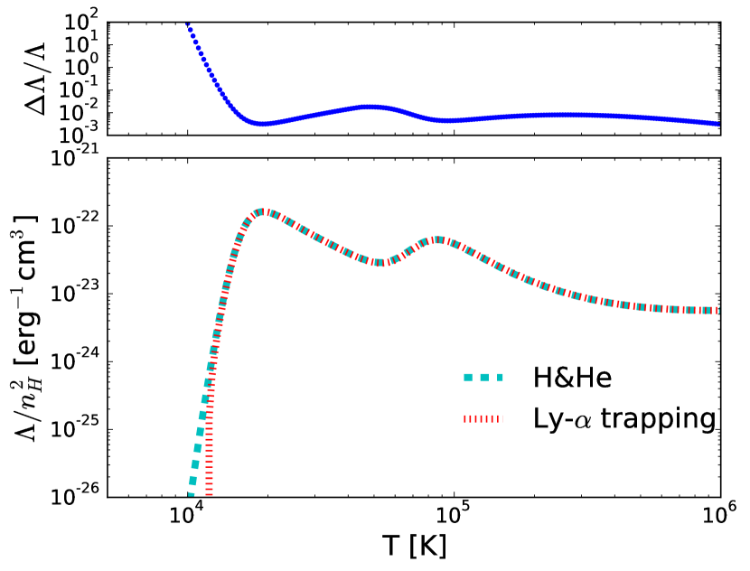
Figure 1: Comparison of overall cooling rates in the optically thin and thick approximations. Top panel: The fractional difference in cooling rates between the two cases. Bottom panel: Dependence of the primordial cooling rate per $n^{2}$ on temperature in the optically-thin limit (blue dashed) and while considering Ly$\alpha$ trapping (red dotted). Significant differences only exist at $T<20,000\;\textrm{K}$ because gas is optically thick to Ly$\alpha$ radiation.

3.1 Radiative cooling with Ly$\alpha$ trapping

The massive seed BH mass is largely influenced by the mass accretion rates into the central gas cloud and any fragmentation that might occur during its catastrophic collapse, prompted by the radiative cooling of a primordial gas. The virial temperature of the candidate halo that hosts massive BH seed formation is $\gtrsim 8000\;\textrm{K}$, which corresponds to a virial mass $M_{\rm vir}\simeq 10^{8}~{}{\textrm{M}_{\odot}}{}[(1+z)/10]^{-3/2}$. For such a contraction to proceed the cooling timescale

$$t_{\rm cool}\simeq\frac{1}{n_{\rm e}^{2}\Lambda(T)}\frac{3\rho kT}{2\mu m_{\rm p}}$$ (9)

must be shorter than or similar to the dynamical time $t_{\rm dyn}=(G\rho)^{-1/2}$ (White & Rees, 1978). Here $\Lambda$ is the cooling function, and $n_{e}$ and $\rho$ are the electron number density and gas density, respectively. Starting at temperatures $T\sim 10^{4}\;\textrm{K}$, hydrogen becomes partially ionized, eventually reaching near complete ionization at $T\sim 1.5\times 10^{4}\;\textrm{K}$. Thus in these halos with virial temperatures near this limit, the assumption that the primordial gas is either completely ionized ($\mu=0.6$) or neutral ($\mu=1.22$), in addition to $n_{\rm e}$, could be inaccurate during the collapse and should be tracked.

At low densities $n\lesssim 100~{}{{\rm cm^{-3}}}$, the use of the optically thin cooling rates is valid. However when Ly$\alpha$ radiation from collisional and recombination processes is extremely attenuated at higher densities, the cooling function $\Lambda$ should decrease as thermal energy cannot be effectively radiated out of the system anymore. When these cooling channels are blocked, a primordial gas can still radiatively cool through the two-photon process.

Figure 1 compares the cooling function of atomic metal-free gas in the optically-thin regime and when the gas is optically-thick to Ly$\alpha$ radiation. The trapped Ly$\alpha$ radiation reduces the cooling rates at $T\lesssim 2\times 10^{4}\;\textrm{K}$, which could result in higher temperatures as the primordial gas cloud collapses. Above this temperature, Ly$\alpha$ trapping and the associated resonance scattering does not occur because spontaneous emission in hydrogen dominates, and furthermore helium de-excitation cooling becomes important at these higher temperatures. Nevertheless, we next investigate this effect further in our Ly$\alpha$ radiative transfer calculations as the system is dynamically collapsing, checking how the thermodynamic properties change during this event.

3.2 Cosmological Halo Collapse: A Basis for Ly$\alpha$ Transfer

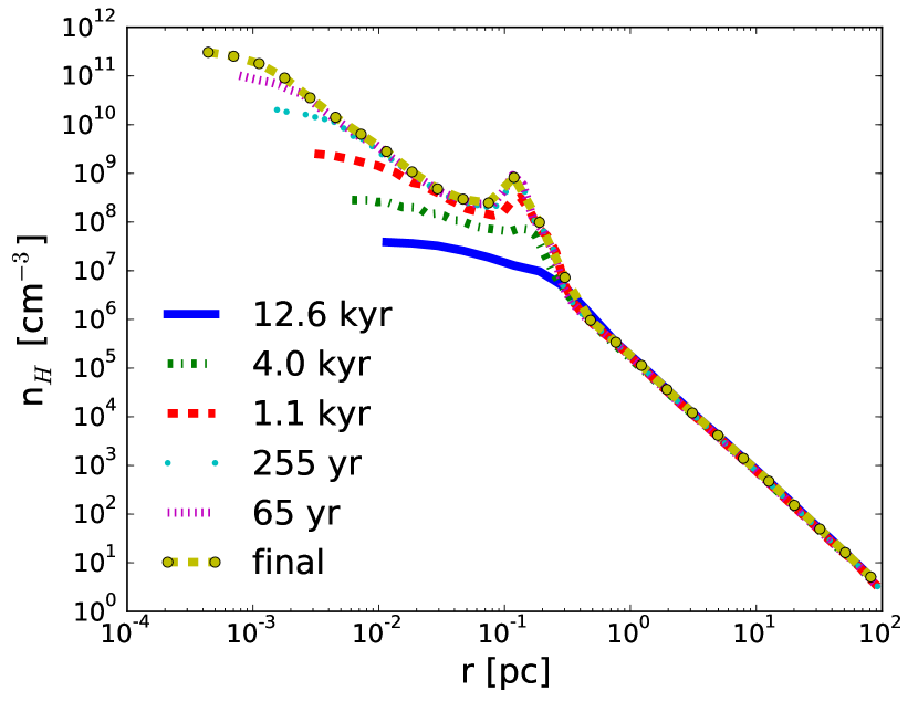
Figure 2: Radially-averaged profiles of gas number density (top) and profiles of electron fraction with respect to number density (bottom) at the final output when the collapse reaches $n_{\rm H}=3\times 10^{11}{{\rm cm^{-3}}}$ and 65, 255, 1,100, 4,000, and 12,600 years before this time. The halo density follows a $r^{-2.2}$ power law, appropriate for an isothermal collapse. The bump at 0.1 pc corresponds to lesser overdensity that has fragmented from the main collapsing cloud. The electron fraction drops with density as free electrons are consumed by recombinations.

We utilize a collapsing halo from a cosmological simulation as the basis for the Monte Carlo radiation transfer calculations, providing a more realistic environment for the propagation medium of the Ly$\alpha$ photons. This halo is the most massive in the simulation domain with a total mass $M_{\rm tot}=5.85\times 10^{7}~{}{\textrm{M}_{\odot}}$ and a virial radius $r_{\rm vir}=782\;\textrm{pc}$ when it catastrophically collapses at $z=14.664$. This halo mass corresponds to a virial temperature $T_{\rm vir}=1.17\times 10^{4}\;\textrm{K}$, which is typical of a metal-free atomic cooling halo that cools and collapses for the first time. The halo does not experience any major mergers for the last 100 Myr of the simulation.

Figure 2 shows the evolution of radially-averaged profiles of the gas number density $n_{\rm H}$ and the average electron fraction at a given $n_{\rm H}$ value. The first density profile depicts the system when the maximum $n_{\rm H}\simeq 10^{7.5}~{}{{\rm cm^{-3}}}$ (AMR level 15), and then the profiles are shown as the maximum density increases by $\sim$1 dex, finally reaching a maximum $n_{\rm H}\simeq 3\times 10^{11}~{}{{\rm cm^{-3}}}$ (AMR level 20). The density profile generally exhibits a power law $\rho\propto r^{-2.2}$ from the virial radius to $\sim 10^{-3}\;\textrm{pc}$. This feature is typical of an isothermal collapse, which happens in this case at $T\simeq 8000\;\textrm{K}$, where the gas cooling is limited to atomic processes in the presence of a strong LW radiation field $J_{21}=10^{5}$. With the isothermal density profile, the inner 1 pc is gravitationally unstable, and its Jeans mass is $\sim 10^{5}~{}{\textrm{M}_{\odot}}$, similar to previous works (e.g. Wise et al., 2008; Regan & Haehnelt, 2009; Shang et al., 2010; Becerra et al., 2015). One exception to the centrally concentrated, spherically symmetric collapse is a clump that fragments $\sim 0.1\;\textrm{pc}$ from the densest point, seen as a bump in the density profile, which initially fragments about 5 kyr before the collapse. The electron fraction in the lower panel of Figure 2 shows that the free electron fraction decreases with density (i.e. radius) as the recombination rate increases with $n^{2}$, eventually saturating at $2\times 10^{-6}$. The electron fraction will play an important role in determining the Ly$\alpha$ emissivity as it is directly related to the electron number density (Equations 5 and 6).

3.3 Monte Carlo Radiation Transfer

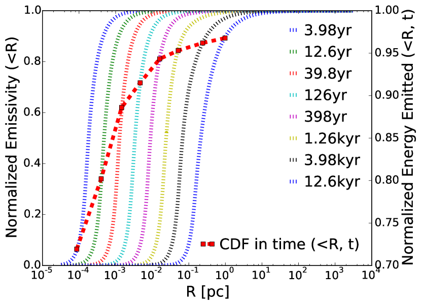
Figure 3: Dotted lines and left axis: Normalized Ly$\alpha$ emissivity cumulative profiles at eight times (see legend) before the final simulation output. Dashed line and right axis: Cumulative amount of Ly$\alpha$ radiation emitted from the time indicated by the intersecting dotted line to 1 Myr before the final output time, i.e. 96% of all Ly$\alpha$ radiation is emitted within 4 kyr of the final collapse.

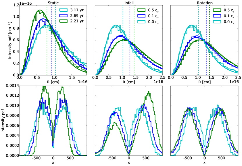
Figure 4: Ly$\alpha$ radiation transfer calculations in the uniform density case with a hydrogen number density $n_{\rm H}=10^{8}~{}{{\rm cm^{-3}}}$. Top row: Ly$\alpha$ radiation intensity as a function of radius for the static case (left), infall case (middle), and rotation case (right), where the vertical lines show the intensity-weighted means. The histograms depict the results from the radiation transport calculation, whereas the smooth curve is a fit to the distribution. The static case shows the radiation propagating outwards, slower than the speed of light due to scattering, at three different times. The infall and rotation cases, shown at $t=3.17\;\textrm{yr}$ ($ct=3\times 10^{16}\;\textrm{cm}$), demonstrate that the bulk motion of the gas allows the radiation to propagate farther as the photons experience a greater Doppler shift when they are re-emitted. Bottom row: The normalized spectra of Ly$\alpha$ radiation for the same cases shown in the top row. In the static case, the Ly$\alpha$ photons shift away from the line center as time progresses, and the infall and rotation cases show the increased Doppler shifts as the gas bulk motion increases.

Before invoking a radiation transport calculation, we first calculate the Ly$\alpha$ emissivity, using Equations (5) and (6), in the collapsing halo at eight different snapshots during the event. The bulk of the emission occurs in the central regions, as expected, and we show the cumulative Ly$\alpha$ luminosity,

$$L_{\rm Lya}(<r,t)=\int_{0}^{r}\left[\eta^{\rm rec}(t)+\eta^{\rm dcol}(t)\right]dV,$$ (10)

as function of radius in Figure 3 with the sphere centered on the densest point. One can see that as the inner region collapses, the source of Ly$\alpha$ emission shrinks as the density increases. When the central object becomes gravitationally unstable 12.6 kyr before the final time, 90% (50%) of the emission comes from the central 1.0 (0.2) pc. This radius decreases gradually with time until a sphere of radius $10^{-3}$ generates 99% of the Ly$\alpha$ radiation at the final time.

As the halo is dynamically collapsing, we can calculate the total Ly$\alpha$ energy being emitted throughout its collapse by numerically integrating Equation (10) from 1 Myr before the final simulation time to the times shown in Figure 3. The red dashed line shows this value, and the differences between adjacent points equal the percentage of total Ly$\alpha$ radiation generated between these two times. For instance, at 4 kyr before the final time, 96% of all Ly$\alpha$ radiation during the collapse is generated after this time, with most of the photons originating within a radius 0.1 pc. This fractional energy decreases with time until 72% of the Ly$\alpha$ radiation originates only 4 yr before the final collapse.

Both the location and timing of the Ly$\alpha$ radiation will aid us in constructing Monte Carlo calculations with the appropriate length and temporal scales. These simulations will explore physical scenarios that gradually increase the realism of the environment through which the Ly$\alpha$ photons propagate. First we will inspect the uniform density case, then the time-independent isotropic case, and finally a collapsing time-dependent isotropic case. The last and most realistic case is used to calculate the effective equation of state, which is an essential ingredient when determining the thermodynamic behavior, and thus possible fragmentation, of the collapsing system.

3.3.1 Uniform density case

Table 1: Fitting parameters for the radiation distribution in the uniform density case

Case	$\log(n_{\rm H}/{{\rm cm^{-3}}})$	$a$	$b_{0}$	$b_{1}$
Static	6	3.46	$1.28\times 10^{10}$	0.732
	7	3.48	$6.67\times 10^{9}$	0.738
	8	3.48	$2.42\times 10^{9}$	0.730
	9	3.50	$4.15\times 10^{9}$	0.731
Infall	6	2.80	$2.04\times 10^{10}$	0.747
	7	2.85	$8.86\times 10^{9}$	0.756
	8	2.61	$3.40\times 10^{9}$	0.750
	9	2.60	$1.24\times 10^{9}$	0.768
Rotation	6	2.77	$1.90\times 10^{10}$	0.749
	7	2.72	$1.02\times 10^{10}$	0.752
	8	2.77	$2.98\times 10^{9}$	0.753
	9	2.78	$1.65\times 10^{9}$	0.757

Notes: The parameters apply to Equation (11). The static case has zero bulk velocity. The parameters for the infall and rotation case are shown only for the $0.5c_{\rm s}$ cases.

The most fundamental case to inspect in a Ly$\alpha$ transfer calculation is a gas parcel with uniform density and temperature. Here we monitor how the radiation propagates from a single impulse originating from a point source at $r=0$. We execute a series of simulations in spherical symmetry with a uniform temperature of 8000 K, which is similar to the temperatures in the atomic cooling halo presented in Section 3.2, and four different hydrogen number densities $\log(n_{\rm H}/{{\rm cm^{-3}}})=(6,7,8,9)$. The top row of Figure 4 shows the radial behavior of the radiation energy distribution in the $n_{\rm H}=10^{8}~{}{{\rm cm^{-3}}}$ case for the static (left panel), infall (middle panel), and rotation (right panel) cases.

The static case, which is shown at three times, $t=(2.21,2.69,3.17)\;\textrm{yr}$ with the last time corresponding to $t=10^{8}\;\textrm{s}$ and a light travel time $ct=3\times 10^{18}\;\textrm{cm}$, have the radial distributions that are well fit with Gamma distributions, valid for the entirety of the simulation time $t<10^{8}\;\textrm{s}$,

$$p(r,t)=\frac{r^{a-1}\,e^{-r/b(t)}}{[b(t)]^{a}\,\Gamma(a)}.$$ (11)

Here $a$ is a constant and controls the distribution width (i.e. the shape parameter), and $b(t)=b_{0}t^{b_{1}}$ varies with time (i.e. the rate parameter) and controls the length of the tail at larger radii. $\Gamma(x)$ is the complete Gamma function, and $t$ is in units of seconds. We do not consider the distribution beyond a light travel time $r=ct$. These parameters are given in Table 1. For such a distribution, the maximum value occurs at $(a-1)b$; the average value is $ab$; the skewness is $2/\sqrt{a}$. Taking the $n_{\rm H}=10^{8}~{}{{\rm cm^{-3}}}$ case as an example, we have $ab=0.281\,t^{-0.272}\times(ct)$. Compared to the optically thin case ($ab=ct$), the Ly$\alpha$ radiation is diluted by a factor of 0.281, and its propagation slows as time progresses, as indicated by the negative exponent. This behavior is apparent in the top-left panel of Figure 4, where the distribution migrates to larger radii with its tail becoming longer. Looking at other densities, the shape parameter $a$ is basically unchanged, which is analogous to having a resonant scattering shell with a constant relative thickness. The bottom row of Figure 4 shows the relative frequencies of the photons. In the static case, the spectrum is symmetric around the line center ($x=0$), which is expected, and obeys the Neufeld (1990) profile. The width of the lines depend on the optical depth of the system and the time elapsed. At early times, the photons are nearest to the line center, and they Doppler shift away from the center as they resonate in the neutral hydrogen medium.

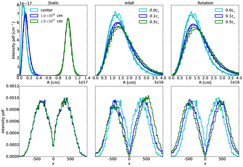
Figure 5: Same as Figure 4 but for the time-independent isotropic case that propagates Ly$\alpha$ radiation through a spherically symmetric halo with its quantities taken from a cosmological simulation. The static case (left) shows the radiation distribution and spectra at $t=10^{8}\;\textrm{s}$ when the photons are generated at the halo center and in two shells with radii $r=10^{16}\;\textrm{cm}$ and $10^{17}\;\textrm{cm}$. The radiation preferentially propagates outward because of the density gradient. The infall (center) and rotation (right) cases are shown at the same time with the photons generated in a shell of radius $r=10^{16}\;\textrm{s}$ for speeds $v/c_{\rm s}=(0.1,0.5)$. Their distributions and spectra show similar behavior as the uniform density case with the photons being Doppler shifted as the velocity increases, resulting in a wider radiation distribution.

Next we inspect the radial distribution of Ly$\alpha$ radiation and its spectra in the infall and rotation cases, which are shown in the middle and right columns of Figure 4. Comparing the spectra of the infall cases with $v_{\rm r}/c_{\rm s}=(0.1,0.5)$ and the static case, we see that the photons are blue-shifted farther away from the line center, which occurs when the infalling gas re-emits the Ly$\alpha$ photons whose relative velocity causes an increase in frequency. Because of the enhanced Doppler shift, the photons scatter less because of the decreased optical depth away from the line center, allowing for the Ly$\alpha$ radiation to propagate farther away from the sphere center, which is seen in a broader radial profile. In the rotation case with $v_{\theta}/c_{\rm s}=(0.1,0.5)$, the photons are symmetrically shifted into the wings of the line, which extends the radiation distribution similar to the infall case. These distributions are still nicely fit with a Gamma distribution (Equation 11) at various number densities and bulk velocities, and we show the fitting parameters in Table 1 alongside the static case. Both infall and rotation cases have larger $b$ parameters, indicating that the radiation is less trapped in the gas.

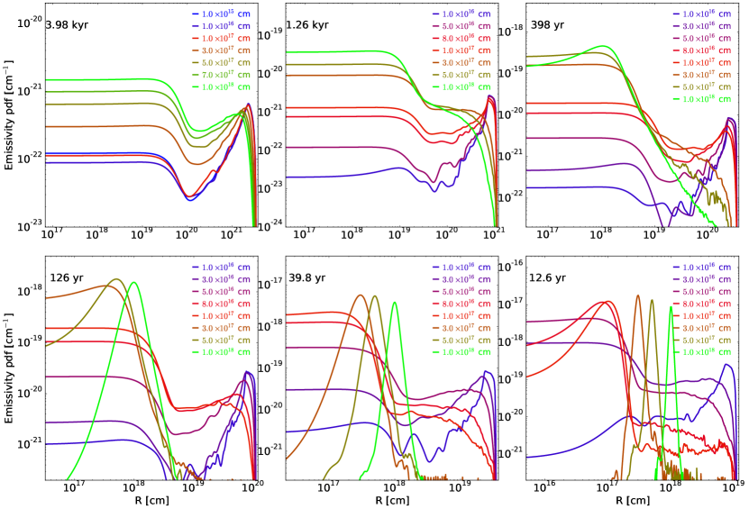
Figure 6: Radial distributions of Ly$\alpha$ emissivity sourced from a subset of individual shells in the time-dependent isotropic case at six different times before the final collapse. The lines are colored by their shell radius and track the propagation from that initial radius to the final state. At early times, there is enough time for the emissivities to reach an equilibrium in the core while some fraction escape into the outer regions of the halo. At later times, the distributions from the larger shells do not have time to propagate far from their origin, while the smaller shells contribute the most to the Ly$\alpha$ radiation field in the inner core with radius 0.1 pc.

Because a single impulse of radiation sourced these radial distributions, we can increase the realism of the calculation by integrating these radiation profiles with respect to time in the range $t=0\rightarrow\mathcal{T}$, which representing the center constantly emitting photons. Integrating Equation (11), we find that the radiation profile transforms into

$$P(r,\mathcal{T})=\int_{0}^{\mathcal{T}}p(r,t)\,dt=\frac{r^{1/(b_{1}-1)}\,\Gamma(a-1/b_{1},(r/b_{0})\,\mathcal{T}^{-b_{1}})}{\mathcal{T}\,b_{1}\,b_{0}^{1/b_{1}}\,\Gamma(a)},$$ (12)

where $\Gamma(x,y)$ is the incomplete Gamma function. The resulting distribution has an intensity-averaged radius $\mathbb{E}(r)=ab/(1+b_{1})$ that is proportional to the distribution coming from a radiation impulse. In this case, the scattering and trapping of Ly$\alpha$ radiation and its diminished radial propagation declines with time as $t^{-\alpha}$, where $\alpha=2.4-2.7$, in the static case.

3.3.2 Time-independent isotropic case

Now that we have established the behavior of Ly$\alpha$ radiation transport in a uniform density and temperature case, we turn our attention to the time-independent isotropic case. Here we consider a spherically symmetric system, taking the radial profiles of density and temperature, along with the average electron fraction as a function of density, from the atomic cooling halo in the cosmological simulation (Section 3.2), 4.0 kyr before the final output when the maximum number density $n_{\rm H}=3\times 10^{8}~{}{{\rm cm^{-3}}}$. In this case, we consider three cases of Ly$\alpha$ radiation generation: from the center of the halo and from two concentric shells with radii $r=10^{16}\;\textrm{cm}$ and $10^{17}\;\textrm{cm}$. We do not utilize the velocity information from the simulation but consider the same velocity setups as the uniform density case: static, infalling, and rotation, where the latter two configurations have $v/c_{\rm s}=(0.1,0.5)$. We allow these photons to propagate according to the scattering radiative transfer equation into the spherically symmetric halo.

Table 2: Fitting parameters for the radiation distribution in the static isotropic case

Case	$r$ [cm]	$a_{0}$	$a_{1}$	$b_{0}$	$b_{1}$
Static	0	$5.99\times 10^{7}$	0.801	$6.90\times 10^{-7}$	2.448
	$10^{16}$	$7.87\times 10^{8}$	0.916	$1.24\times 10^{-7}$	2.525
	$10^{17}$	$6.48\times 10^{9}$	0.996	$1.21\times 10^{-3}$	2.162
Infall	0	$3.46\times 10^{2}$	0.259	$2.26\times 10^{6}$	1.180
	$10^{16}$	$3.98\times 10^{2}$	0.265	$1.71\times 10^{6}$	1.193
	$10^{17}$	$7.48\times 10^{2}$	0.291	$3.44\times 10^{6}$	1.162
Rotation	0	$2.98\times 10^{2}$	0.248	$1.90\times 10^{6}$	1.156
	$10^{16}$	$3.82\times 10^{2}$	0.280	$2.02\times 10^{6}$	1.176
	$10^{17}$	$8.44\times 10^{2}$	0.301	$2.98\times 10^{6}$	1.142

Notes: The parameters apply to Equation (11) but with $a(t)=a_{0}\,t^{-a_{1}}$. For $r=0$, the Ly$\alpha$ radiation originates at the halo center, and for the non-zero radii, it originates from shells of those radii. The static case has zero bulk velocity. The parameters for the infall and rotation case are shown only for the $0.5c_{\rm s}$ cases. The associated fits are accurate for $t<10^{9}\;\textrm{s}$.

Figure 5 shows the resulting radiation radial distribution (top panels) and spectra (bottom panels) at a time $t=10^{8}\;\textrm{s}=3.17\;\textrm{yr}$, corresponding to a light travel time $ct=3\times 10^{18}\;\textrm{cm}$. Focusing first on the static case (left column), the Ly$\alpha$ radiation propagates away from the center with a maximum at $8\times 10^{15}\;\textrm{cm}$, while the photons from the radiating shells at $r=10^{16}\;\textrm{cm}$ and $10^{17}\;\textrm{cm}$ preferentially migrates outward because of the density gradient. These distributions are again well fit with a Gamma distribution (Equation 11), similar to the uniform density case but with $a(t)=a_{0}t^{-a_{1}}$ instead of being a constant. The fitting parameters for the three cases are given in Table 2. The preference toward outward propagation can be quantified by inspecting the skewness ($2/\sqrt{a}$) of these distributions, which are in the range 0.2–0.4. The spectra for the central and shell sources have similar spectra, as expected, because they are shown at the same integration time and the velocities are the same.

Both the radial distribution of Ly$\alpha$ radiation and the spectra of the infall and rotation cases behave similarly to their counterparts in the uniform density case. The middle and right columns of Figure 5 show these respective cases at a time $t=10^{8}\;\textrm{s}$ with the photons being generated in a shell of radius $r=10^{16}\;\textrm{cm}$. We also consider the cases where photons are generated in the center and a larger shell of radius $10^{17}\;\textrm{cm}$, whose fitting parameters are shown in Table 2 but not shown in the Figure. The relative velocities of the gas cause a Doppler shift, allowing the photon frequencies to migrate away from the line center, with a tendency toward a blueshift in the infall case and symmetric shifts in the rotation case. This effect increases their mean free path, extending the radial profiles. As the photons propagate outward into the more diffuse regions (recall $\rho\propto r^{-2.2}$) of the halo, they will scatter less frequently, eventually free streaming away from the halo center.

3.3.3 Time-dependent isotropic case

We now consider the case where the halo is dynamically collapsing, whereas previously we restricted the integration times to $10^{8}\;\textrm{s}$ that is comparable to the light-crossing time of the inner parsec. This time-dependent calculation is similar to the time-independent calculation; however we utilize six outputs from the cosmological simulation that are evenly log-spaced in time, starting at 3.98 kyr before the collapse. The density profiles are approximately isothermal with $\rho\propto r^{-2.2}$ at all times with the maximum density increasing from $3\times 10^{8}~{}{{\rm cm^{-3}}}$ to $3\times 10^{11}~{}{{\rm cm^{-3}}}$ during this time. At each time, 20 shells radiate Ly$\alpha$ photons, which are equally log-spaced in radius ranging from $10^{14}\;\textrm{cm}$ to $10^{19}\;\textrm{cm}$. The output times $t_{i}$ are given in Table 3. The largest shell encloses nearly all of the Ly$\alpha$ radiation that was depicted in Figure 3. The major improvement upon the previous cases is that we integrate over the resulting radiation distribution from each shell to compute a cumulative radiation distribution for the entire halo.

Starting at the earliest time, the shells radiate for a time equal to the duration between outputs (i.e. $t_{i}-t_{i+1}$). We track the radial distribution of the photons from each shell, where Figure 6 shows a subset of the 20 shells, allowing us to inspect the propagation behavior from each radiation origin. At the earliest time (3.98 kyr), the radial distributions from each shell have similar shapes. They have plateaus at small radii, which have reached an equilibrium between emission and scattering out of the center. The local maxima at $r\simeq 1-2\times 10^{21}\;\textrm{cm}$ represent the photons that have escaped the inner regions by scattering many times and driving the frequency into the wings of the spectrum, and they are freely streaming outward through the diffuse outer regions. As the collapse progressively accelerates, the dynamical time decreases, giving less time for the photons to propagate through the pre-galactic medium. This behavior can be seen through the steadily decreasing radiation distribution at large radii at $t=1260$ and $398\;\textrm{yr}$ for the largest shells. Eventually in the latter times, the distributions for the largest shells transform into Gamma distributions as the integration times shorten to $\sim 10^{8}\;\textrm{s}$. However for the radiation originating from intermediate radii (e.g. $r=3\times 10^{16}\;\textrm{cm}$ and $5\times 10^{16}\;\textrm{cm}$ at $t=12.6\;\textrm{yr}$), the Ly$\alpha$ photon distribution still have a plateau at small radii.

3.4 Effective equation of state with Ly$\alpha$ scattering

Table 3: Output times and range of radii of the radiating shells in the equation of state calculation

Case $i$	Time $t_{i}$ [yr]	Shell radii range [$10^{16}$ cm]
0	3,980	10 – 100
1	1,260	5 – 100
2	398	3 – 100
3	126	2 – 100
4	39.8	1 – 100
5	12.6	1 – 100

The radiation distributions from individual shells informs us how the radiation transports given an origin, but at some given time, the overall Ly$\alpha$ emissivity distribution is the key quantity in determining the coupling between the Ly$\alpha$ photons and the neutral medium. Ultimately, we can compare the radiation distribution from the transport calculation to the optically-thin (free streaming) case to calculate the reduction in the radiative cooling rate from collisional excitations and ionizations.

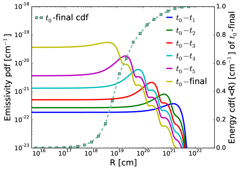
Figure 7: The total Ly$\alpha$ emissivity integrated (Equation 13) from all of the shells shown in Figure 6 and all times from $t_{0}$ to $t_{i}$. The yellow (top) solid line shows the Ly$\alpha$ emissivity at the final time of the simulation. The dashed line with square points depicts the cumulative Ly$\alpha$ emissivity at the final time with 50% (90%) of it being contained within 3 pc (50 pc).

Figure 7 shows the resulting Ly$\alpha$ normalized emissivities as a function of radius at several times. We only consider the shells within the radius range given in Table 3 to reduce the computation, and we have found that the shells outside the given ranges do not contribute to the overall emissivity. We first start by calculating the total emissivity from the first time interval ($t_{0}\rightarrow t_{1}$), shown as the blue line in the Figure. Then at the next output time $t_{2}$, we calculate the total emissivity in the next interval ($t_{1}\rightarrow t_{2}$) and add it to the previous profile. This process is repeated until we reach the final output simulation time. In other words, at some time $t_{n}$, we construct the time-integrated emissivity profile by discretely adding each time interval:

$$\eta^{\rm total}(t_{\rm n},r)=\sum_{i}^{n}\eta(t_{\rm i}\rightarrow t_{\rm n},r)=\sum_{i}^{n}\sum_{\rm shells}\eta^{s}(t_{\rm i}\rightarrow t_{\rm n},r)$$ (13)

where $n$ is an integer in the interval $[0,5]$, and its maximum corresponds to the number of simulation outputs considered. During the summation, we smooth the Monte Carlo results with the kernel density estimation (KDE) method in scipy with the default parameters (Jones et al., 2001). However because $n$ is small, we have numerical artifacts at large radii from the addition of the local maxima from previous times (i.e. $i<n$), but they do not affect the accuracy of the final emissivity profile.

As the halo collapses, the Ly$\alpha$ emissivity progressively becomes more centrally concentrated because of the increased photon generation rate from the higher densities. At the final time (yellow line in Figure 7) when the maximum density $n_{\rm H}=3\times 10^{11}~{}{{\rm cm^{-3}}}$, we see that the bulk of the Ly$\alpha$ is contained within $r<10^{19}\;\textrm{cm}\simeq 3\;\textrm{pc}$ that is approximately the Jeans length of the central object. At this radius, the number density $n_{\rm H}\simeq 10^{4}~{}{{\rm cm^{-3}}}$, above which the medium becomes prone to Ly$\alpha$ scattering and a reduction in radiative cooling. Also we show cumulative emissivity profile within a radius $R$

$$\eta(<R,t_{\rm final})=\int_{0}^{R}\eta^{\rm total}(t_{\rm final})\,dV$$ (14)

in Figure 7 as the dashed cyan line, illustrating that 50% (90%) of the Ly$\alpha$ radiation is contained within $\sim$3 pc (50 pc).

Finally with the Ly$\alpha$ emissivity profile $\eta^{\rm total}$ at the final time $t_{\rm final}$, we can determine how much the radiative cooling is reduced. We first convert this profile into a function of density by using the halo radial density profile (Figure 2). Then we take the difference between our Monte Carlo radiation transport result and the optically-thin emissivity $n^{\rm src}$ (see Equations 5 and 6) and convert that into an effective heating rate as a function of density. Figure 8 depicts the resulting effective equation of state up to a number density $n_{\rm H}=10^{12}~{}{{\rm cm^{-3}}}$ that is approximately the maximum density in the simulation. Here we take the initial temperature at $n=0.1~{}{{\rm cm^{-3}}}$ to be $T=9000\;\textrm{K}$. As the gas condenses, Ly$\alpha$ radiation becomes more coupled to the neutral gas, reducing its cooling rate with respect to the optically-thin rate, resulting in the gas gradually heating to $5\times 10^{4}\;\textrm{K}$ at $n_{\rm H}=3\times 10^{4}~{}{{\rm cm^{-3}}}$. However at higher densities (smaller radii), the gas cools back to $10^{4}\;\textrm{K}$ because the Ly$\alpha$ emissivity plateaus within 3 pc, corresponding to $n_{\rm H}=10^{4}~{}{{\rm cm^{-3}}}$ in the density profile. This heating from partially Ly$\alpha$ trapping at moderate densities is in stark contrast to the optically-thin case, where the gas slowly cools from 9000 K to 7000 K (green dashed line). The gas starts to cool because the optically thin cooling rate increases as $n_{\rm e}n_{\rm HI}$ or $n_{\rm e}n_{\rm HII}$ for collisional excitation and recombination, respectively, while the Ly$\alpha$ emissivity from the Monte Carlo calculation has plateaued. The combination of this saturation and increasing optically-thin cooling rate ultimately results in the dense gas cooling back below $10^{4}\;\textrm{K}$. We then differentiate this effective equation of state to obtain the adiabatic index $\gamma=1+d\ln T/d\ln\rho$ for an ideal gas (red dashed line in Figure 8). As the gas heats, $\gamma$ increases from unity to $\sim$4/3 at $n_{\rm H}=10^{4}~{}{{\rm cm^{-3}}}$, suddenly decreases to $\sim$4/5 at $n_{\rm H}=10^{6}~{}{{\rm cm^{-3}}}$, and then recovers back to unity with increasing density.

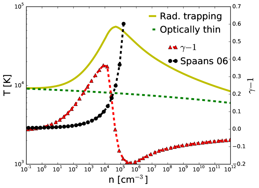
Figure 8: Left axis: Effective equation of state derived from the Ly$\alpha$ radiation transfer calculation (solid yellow) and optically-thin cooling rates (green dashed). The gas heats from the initial temperature of 9,000 K to 50,000 K by $n_{\rm H}=3\times 10^{4}~{}{{\rm cm^{-3}}}$ from Ly$\alpha$ trapping and then cools to $10^{4}\;\textrm{K}$ at higher densities. Right axis: Adiabatic index $\gamma-1$ of the effective equation of state from this work (red dashed) that well describes the suppressed Ly$\alpha$ cooling from radiation trapping and from the analytical work of Spaans & Silk (2006, black dashed) that diverges above $10^{5}~{}{{\rm cm^{-3}}}$ where it should be limited to 5/3.

In Figure 8, we compare our equation of state to the one analytically derived from spherical symmetry in Spaans & Silk (2006), shown as a dashed black line, that has the form

$$\gamma-1\approx-\frac{\tfrac{1}{2}+\tfrac{7}{18}Bn_{1}^{7/18}}{\log(Cn_{1}^{0.5})+Bn_{1}^{7/18}},$$ (15)

where $B\approx 0.47\;\textrm{cm}^{7/6}$, $C\approx 10^{-34}\;\textrm{cm}^{3/2}$, and $n_{1}$ is 100 times the number density in units of cm^-3 (see Latif et al., 2011, for the motivation to boost $n_{1}$). This result describes a smooth but quick transition from isothermal to adiabatic ($\gamma=5/3$), but it diverges for high number densities and must be limited to 5/3 at high densities. The bulk of the increase in $\gamma$ comes between $\log(n_{\rm H}/\textrm{cm}^{-3})=4-5$, whereas our results starts to increase from unity around $100~{}{{\rm cm^{-3}}}$, only reaching $\sim$4/3 at $10^{4}~{}{{\rm cm^{-3}}}$. Our effective equation of state is still valid for high number densities when the cloud is optically thick, whereas the Spaans & Silk result breaks down and must be approximated with an adiabatic equation of state.

4 Conclusions and Discussion

We have utilized a suite of Monte Carlo Ly$\alpha$ radiative transfer calculations to study the effects of Ly$\alpha$ radiation trapping in a metal-free pre-galactic halo, which we have extracted from an AMR cosmological simulation, using Enzo. In this paper, we have quantified the delayed radiation propagation and associated reduced radiative cooling within these objects that could be precursors of direct collapse black holes or dense stellar clusters. From these calculations, we have estimated an effective equation of state for this collapsing primordial gas. The key results of this paper are summarized below.

1. By introducing a Ly$\alpha$ model, we found that the primordial cooling rates are reduced below 20,000 K at densities above 100 cm^-3. Above this temperature, cooling from spontaneous emission in hydrogen dominates, and below this density, the gas is effectively optically thin to Ly$\alpha$ radiation.

2. The majority of the Ly$\alpha$ photons are generated within a radius of $\sim$1 pc and $\sim$1 kyr before the collapse of the central primordial gas cloud inside of a pre-galactic atomic cooling halo. This gas is optically thick to Ly$\alpha$ radiation, which is trapped within the cloud, but it eventually escapes from the cloud. Thus, the optically-thin cooling rates overestimate the actual cooling behavior of this collapsing gaseous object.

3. When we consider a static density field, whether it be uniform or an isothermal profile, the Ly$\alpha$ radiation outward propagation is delayed by resonance scattering, resulting in a emissivity radial profile that is well described by a Gamma distribution. Subsonic inward or rotational bulk velocities allow the Ly$\alpha$ photons to shift into the wings of the line profile but have little effect on reducing the amount of trapping.

4. We apply these results to a dynamically collapsing halo in a discrete manner, where we find that the Ly$\alpha$ radiation is still trapped. However, the radiative cooling rates are not fully suppressed with the adiabatic index rising from unity to $\sim$4/3 at $n_{\rm H}=10^{4}~{}{{\rm cm^{-3}}}$ with the temperature increasing to 50,000 K at the same number density. At higher densities, the Ly$\alpha$ emissivity saturates while cooling rates from collisional excitation and recombination increase as $n^{2}$, allowing the gas to cool back to 10,000 K. This thermodynamic track results in a heated envelope with a cooled core that will form either a dense stellar cluster or a supermassive star, eventually forming a massive black hole seed.

We have seen that Ly$\alpha$ radiation trapping alters the thermal properties of the collapsing system, which will change its Jeans mass, which ultimately controls the fragmentation mass scales and resulting collapsed object. The Bonnor-Ebert mass (Bonnor, 1956; Ebert, 1955) considers an external pressure $P_{\rm ext}$ around an isothermal gaseous cloud, which is given by

$$M_{\rm BE} =1.18\frac{c_{\rm s}^{4}}{G^{3/2}}P_{\rm ext}^{-1/2}\;{\textrm{M}_{\odot}}$$ (16)

$$\simeq 20T^{3/2}n^{-1/2}\mu^{-2}\gamma^{2}\;{\textrm{M}_{\odot}}$$ (17)

where the second expression is calculated by setting the external pressure to the local pressure. Previous studies of the direct collapse black hole pre-cursors become Jeans unstable at a Bonnor-Ebert mass around $10^{5}~{}{\textrm{M}_{\odot}}$ at a radius of $\sim$1 pc (e.g. Bromm & Loeb, 2003; Wise et al., 2008; Regan & Haehnelt, 2009), which is approximately where we find the primordial gas to be prone to Ly$\alpha$ trapping. We find that the gas heats to 50,000 K at this scale that is 5–6 times larger than the typical 8000 K temperature found in studies using optically-thin cooling rates. This heating increases the Bonner-Ebert mass at this scale by an order of 10–15, which will hinder the initial collapse until the central object can accumulate additional gas. However after the cloud becomes gravitationally unstable, it will cool back down to 8,000–10,000 K, resulting in a cool dense core surrounded by an envelope that is 5 times hotter. This additional external pressure may drive a decrease in the Bonnor-Ebert mass at higher densities.

One shortcoming of our work is the post-processing treatment of the Ly$\alpha$ radiation transport, where the additional heating does not affect the collapse. In the time-dependent case, we utilized the temperature profile from the cosmological simulation that was calculated with the optically-thin cooling rates. But any Ly$\alpha$ feedback will change the gas temperature and thus neutral fraction that will ultimately alter the Ly$\alpha$ radiation field. When the gas is heated above the optically-thin solution, the Ly$\alpha$ photons will scatter to the wings of the line profile faster and overall will have longer mean free path. Additionally, we have assumed spherical symmetry, whereas in a full three-dimensional setup with coupled Ly$\alpha$ transfer anisotropic structures, such as bubbles or channels, can form during the collapse (e.g. Smith et al., 2015), which could have similar anisotropic behavior as ionizing radiation transport in massive star formation (e.g. Krumholz et al., 2009; Rosen et al., 2014). This anisotropy may alter the accretion flows onto and through the collapsing gas cloud. For instance, Ly$\alpha$ trapping may favor some directions than others, creating warmer channels and inhibiting any accretion through those solid angles.

Such feedback loops would create a complex interplay between accretion flows, shocking onto the Jeans unstable gas cloud, Ly$\alpha$ radiation trapping, and the resulting thermal and hydrodynamic response. This will likely alter the angular momentum and entropy of the infalling gas and could have an effect on the outcome of the collapsing object – the spin and mass of a direct collapse black hole, or the star formation efficiency and size of a dense stellar cluster. As computational methods and hardware improve, it is becoming feasible to perform Ly$\alpha$ radiation transport coupled with the hydrodynamics to resolve these complexities arising from the aforementioned feedback processes (e.g. see a discussion in Smith et al., 2017) that will bring us closer to resolving the nature of the initial central object of these highly irradiated, metal-free, pre-galactic halos.

Appendix A Cooling with approximate Ly$\alpha$ radiative transfer

A.1 Average number of scattering events

Table 4: Coefficients $A_{ij}$ for the exponential fit to the number of scattering events in Equation (27)

	$i=0$	$i=1$	$i=2$	$i=3$	$i=4$	$i=5$
$j=0$	2.597(0)	1.193(0)	4.021(–2)	2.375(–3)	8.825(–5)	–6.167(–6)
$j=1$	–2.000(0)	–3.342(–1)	–9.067(–3)	–3.954(–4)	1.008(–5)
$j=2$	3.400(–1)	3.150(–2)	7.111(–4)	2.748(–7)
$j=3$	–2.422(–2)	–1.351(–3)	–1.157(–5)
$j=4$	8.436(–4)	2.059(–5)
$j=5$	–1.139(–5)

Note: The values are in scientific notation with the exponent in parentheses.

We base our treatment of Ly$\alpha$ radiation trapping in the radiative cooling rate calculation described and presented in Sections 2.1 and 3.1, respectively, on the Omukai (2001) model. In order to calculate the average number of scattering events before escaping the system, we solve the radiative transfer equation for Ly$\alpha$ photons with the Eddington approximation in the isotropic limit (Adams et al., 1971) that describes the evolution of intensity $J$ as a function of optical depth $\tau$ and frequency shift $x\equiv(\nu-\nu_{0})/\Delta\nu_{\rm D}$ as

$$\frac{\nabla^{2}J(\tau,x)}{3H^{2}(a,x)}=J(\tau,x)-\int_{-\infty}^{\infty}J(\tau,x^{\prime})\,q(x,x^{\prime})\,dx^{\prime}-S(\tau,x),$$ (18)

where $H$ is the normalized Voigt profile (Equation 4). Recall that $a\equiv A_{12}/4\pi\Delta\nu_{\rm D}$ (Section 2.1). Here $q(x,x^{\prime})$ is the normalized redistribution function that describes the frequency shifts during scattering events in the atom’s rest frame (Hummer, 1962). The source function $S(\tau,x)$ describes the generation of Ly$\alpha$ radiation at some optical depth and frequency. Using a Taylor expansion of the redistribution functions (e.g. Adams et al., 1971; Harrington, 1973; Rees & Ostriker, 1977), the radiation transfer equation can be formulated as a Poisson equation,

$$\frac{\partial^{2}J}{\partial\tau^{2}}+\nabla^{2}J=-3\frac{S(\tau,x)}{4\pi}.$$ (19)

The equation is solved in spherical symmetry with the boundary condition

$$\frac{\partial J(x,\tau)}{\partial\tau}=-\frac{3}{2}H(a,x)J(\tau,x),$$ (20)

describing a system with $\tau=0$ at the center and $\tau=\tau_{0}$ at the outer boundary $r=R$. Considering an isotropic source at some optical depth $\tau_{\rm s}$, the analytical solution (for the complete derivation, see Appendix C in Dijkstra et al., 2006) to Equation (19) is,

$$J(\tau,\sigma)=\frac{\sqrt{6}}{16\pi^{2}R}\frac{1}{\tau_{0}\tau\tau_{\rm s}}\sum_{n=1}^{\infty}\sin(\lambda_{\rm n}\tau)\sin(\lambda_{\rm n}\tau_{\rm s})\frac{\exp(-\lambda_{\rm n}|\sigma|)}{\lambda_{\rm n}},$$ (21)

where $\sigma\equiv(2\pi/27)^{1/2}x^{3}/a$. The values $\lambda_{\rm n}$ are the coefficients in the solution to the equation,

$$\frac{d^{2}J}{d\tau^{2}}+\lambda^{2}J=0$$ (22)

that has solutions in the form $J_{n}=A\cos(\lambda_{\rm n}\tau)$ (Unno, 1952; Harrington, 1973). After determining the values of $\lambda$ and thus the solution to $J$, it can be integrated from the center to the optical depth $\tau_{s}$ and compared to the intensity $J$ at the outer boundary. The respective ratio of these two quantities relates the number $N_{\rm sc}$ of scatterings inside a sphere with optical depth $\tau_{s}$ to the total number $N_{\rm bd}$ of photons emitted from boundary $\tau_{0}$

$$\frac{N_{\rm sc}(x,\tau_{s})}{N_{\rm bd}(x,\tau_{s})} =\frac{\int_{0}^{\tau_{0}}4\pi\tau^{2}J(\tau,\sigma)\,d\tau}{J(\tau_{0},\sigma)}$$ (23)

$$=\frac{\mathcal{L}(x,\tau_{0},\tau_{\rm s})/[2i\tau_{0}A^{2}(x,\tau_{0})]}{\sin(\pi\tau_{\rm s}/\tau_{0})/\{[3H(a,x)][\cos(\pi\tau_{\rm s}/\tau_{0})+\cosh(\sigma/\tau_{0})]\}},$$

where

$$\mathcal{L}(x,\tau_{0},\tau_{\rm s})\equiv\textrm{Li}_{2}[A(x,\tau_{0})\,(|\sigma|-i\tau_{\rm s})]-\textrm{Li}_{2}[-A(x,\tau_{0})\,(|\sigma|+i\tau_{\rm s})]$$ (24)

and

$$A(x,\tau_{0})=\frac{\pi}{\tau_{0}}\left(1-\frac{2}{3H(a,x)\tau_{0}+2}\right).$$ (25)

The function $\textrm{Li}_{n}(z)\equiv\sum_{k=1}^{\infty}(z^{k}/k^{n})$ is an $n=2$ polylogarithmic function defined in the complex plane. From this solution, we can integrate over the frequency $x$ (or its equivalent $\sigma$) and optical depth $\tau_{s}$ from the center to the boundary, determining the average number of scatterings for a photon escaping from the system to be

$$N_{\rm esc}=\frac{3}{\tau_{0}^{3}}\int_{0}^{\tau_{0}}\frac{\int_{-\infty}^{\infty}N_{\rm sc}(x,\tau_{\rm s})\,dx}{\int_{-\infty}^{\infty}N_{\rm bd}(x,\tau_{\rm s})\,dx}\tau_{\rm s}^{2}\,d\tau_{\rm s}.$$ (26)

This expression for the average number $N_{\rm esc}$ of scatterings cannot be solved analytically, so we numerically integrate it for 1600 equally log-spaced pairs of temperature $T$ in the range of $10^{3}-10^{9}\;\textrm{K}$ (corresponding to some $\Delta\nu_{\rm D}$) and optical depth $\tau_{0}$ in the range $10^{3}-10^{6}$. We fit these numerical results to the two-variable exponential polynomial function

$$\frac{N_{esc}(T,\tau_{0})}{\tau_{0}}=\sum_{i,j}^{i+j\leq 5}\exp\left[A_{\rm ij}\left(\ln T\right)^{i}\left(\ln\tau_{0}\right)^{j}\right]$$ (27)

with the coefficients $A_{\rm ij}$ given in Table 4.

A.2 Radiation emission in a two-level system

We simplify the Ly$\alpha$ emission process by considering a two-level system because the spontaneous transitions from more excited states reside in the optically thin regime (Shang et al., 2010). The number density of the first excited state is related to the ground state by

$$\frac{n_{2}}{n_{1}}=\frac{C_{12}+(g_{2}/g_{1})u_{\nu}A_{21}}{C_{21}+(1+u_{\nu})A_{21}},$$ (28)

where $C_{\rm ij}=n_{\rm e}k_{\rm ij}(\textrm{e})+n_{\rm H}k_{\rm ij}(\textrm{H})$ is the collisional de-excitation rate by free electrons and hydrogen atoms, and $g_{n}=2n^{2}$ is the statistical weight (e.g. Tielens & Hollenbach, 1985; Omukai, 2001). The quantity

$$u_{\nu}=\frac{c^{2}}{2hv_{21}^{3}}J_{\rm cont}(\nu_{21})\gg 1$$ (29)

is related to the incoming photon flux at the energy difference $E_{21}=h\nu_{21}=10.2\;\textrm{eV}$ between the states. The population density of the excited state (Equation 28) will change through collisional processes and spontaneous emission

$$\frac{dn_{2\rightarrow 1}}{dt}=k_{21}(\textrm{e})n_{2}n_{\rm e}+k_{21}(\textrm{H})n_{2}n_{1}+A_{21}n_{2},$$ (30)

and the associated cooling rate per unit volume is reduced by the number of scatterings (Equation 27),

$$\Lambda_{2\rightarrow 1}=\frac{h\nu_{21}}{N_{\rm esc}}\frac{dn_{2\rightarrow 1}}{dt}.$$ (31)

We use the collisional coefficient rates from Omukai (2001):

$$k_{21}(\textrm{e})=1.155\times 10^{-8}\frac{\sqrt{\beta(\beta+1)}}{\beta+0.28}\;\textrm{cm}^{3}\;\textrm{s}^{-1},$$ (32)

$$k_{21}(\textrm{H})=1.454\times 10^{-15}\frac{T^{1/2}+1.693\times 10^{-5}\,T^{3/2}}{1+8.46\times 10^{-17}\,T^{2}}\;\textrm{cm}^{3}\;\textrm{s}^{-1},$$ (33)

where $\beta\equiv E_{21}/kT$. In the temperature range $T=8-10\times 10^{3}\;\textrm{K}$, radiation originating from the two-photon process is in the optically thin regime, but we need to consider it in the model to obtain accurate electron states for the first excited state. The ratio between the $2s$ and $2p$ states is given by

$$\frac{n_{\rm 2s}}{n_{\rm 2p}}=\frac{g_{\rm 2s}}{g_{\rm 2p}}\frac{C_{\rm 2s2p}}{C_{\rm 2s2p}+A_{\rm 2s1s}},$$ (34)

where $(g_{\rm 2s},g_{\rm 2p})=(2,6)$, and $A_{\rm 2s1s}=8.23\;\textrm{s}^{-1}$. The collision rate can be described with the fit (Omukai, 2001)

$$C_{\rm 2s2p}=6.21\times 10^{-4}T^{-1/2}\ln(5.7T)\left[1+\frac{0.78}{\ln(5.7T)}\right]n(\textrm{e})\;\textrm{s}^{-1}.$$ (35)

Lastly, the Einstein A-coefficient associated with spontaneous emission for the 2p $\rightarrow$ 1s and 2s $\rightarrow$ 1s transitions are respectively

$$A_{21}=\frac{n_{\rm 2p}}{n_{2}}A_{\rm 2p1s}\quad\textrm{and}\quad A_{\rm 2ph}=\frac{n_{\rm 2s}}{n_{2}}A_{\rm 2s1s},$$ (36)

resulting in the cooling rate from the two-photon process

$$\Lambda_{\rm 2ph}=h\nu_{21}A_{\rm 2ph}n_{\rm 2s}$$ (37)

References

- Abel et al. (1997) Abel T., Anninos P., Zhang Y., Norman M. L., 1997, New Astron., 2, 181
- Adams (1971) Adams T. F., 1971, ApJ, 168, 575
- Adams et al. (1971) Adams T. F., Hummer D. G., Rybicki G. B., 1971, J. Quant. Spectrosc. Radiative Transfer, 11, 1365
- Agarwal & Khochfar (2015) Agarwal B., Khochfar S., 2015, MNRAS, 446, 160
- Agarwal et al. (2014) Agarwal B., Dalla Vecchia C., Johnson J. L., Khochfar S., Paardekooper J.-P., 2014, MNRAS, 443, 648
- Ahn et al. (2002) Ahn S.-H., Lee H.-W., Lee H. M., 2002, ApJ, 567, 922
- Alexander & Natarajan (2014) Alexander T., Natarajan P., 2014, Science, 345, 1330
- Alvarez et al. (2009) Alvarez M. A., Wise J. H., Abel T., 2009, ApJ, 701, L133
- Anninos et al. (1997) Anninos P., Zhang Y., Abel T., Norman M. L., 1997, New Astronomy, 2, 209
- Barnes & Haehnelt (2010) Barnes L. A., Haehnelt M. G., 2010, MNRAS, 403, 870
- Becerra et al. (2015) Becerra F., Greif T. H., Springel V., Hernquist L. E., 2015, MNRAS, 446, 2380
- Begelman et al. (2006) Begelman M. C., Volonteri M., Rees M. J., 2006, MNRAS, 370, 289
- Bonnor (1956) Bonnor W. B., 1956, MNRAS, 116, 351
- Bromm & Loeb (2003) Bromm V., Loeb A., 2003, ApJ, 596, 34
- Bromm et al. (2003) Bromm V., Yoshida N., Hernquist L., 2003, ApJ, 596, L135
- Bryan et al. (1995) Bryan G. L., Norman M. L., Stone J. M., Cen R., Ostriker J. P., 1995, Computer Physics Communications, 89, 149
- Cen (1992) Cen R., 1992, ApJS, 78, 341
- Colella & Woodward (1984) Colella P., Woodward P. R., 1984, Journal of Computational Physics, 54, 174
- Davies et al. (2011) Davies M. B., Miller M. C., Bellovary J. M., 2011, ApJ, 740, L42
- Dijkstra et al. (2006) Dijkstra M., Haiman Z., Spaans M., 2006, ApJ, 649, 14
- Dijkstra et al. (2008) Dijkstra M., Haiman Z., Mesinger A., Wyithe J. S. B., 2008, MNRAS, 391, 1961
- Ebert (1955) Ebert R., 1955, Z. Astrophys., 37, 217
- Eisenstein & Hut (1998) Eisenstein D. J., Hut P., 1998, ApJ, 498, 137
- Fan (2006) Fan X., 2006, New Astron. Rev., 50, 665
- Glover (2015) Glover S. C. O., 2015, MNRAS, 451, 2082
- Glover & Abel (2008) Glover S. C. O., Abel T., 2008, MNRAS, 388, 1627
- Gronke et al. (2015) Gronke M., Bull P., Dijkstra M., 2015, ApJ, 812, 123
- Hahn & Abel (2011) Hahn O., Abel T., 2011, MNRAS, 415, 2101
- Hamilton (1940) Hamilton D. R., 1940, Physical Review, 58, 122
- Harrington (1973) Harrington J. P., 1973, MNRAS, 162, 43
- Herrmann et al. (2007) Herrmann F., Hinder I., Shoemaker D., Laguna P., Matzner R. A., 2007, ApJ, 661, 430
- Hinshaw et al. (2013) Hinshaw G., et al., 2013, ApJS, 208, 19
- Hummer (1962) Hummer D. G., 1962, MNRAS, 125, 21
- Hunter (2007) Hunter J. D., 2007, Computing In Science & Engineering, 9, 90
- Inayoshi et al. (2016) Inayoshi K., Haiman Z., Ostriker J. P., 2016, MNRAS, 459, 3738
- Jeon et al. (2012) Jeon M., Pawlik A. H., Greif T. H., Glover S. C. O., Bromm V., Milosavljević M., Klessen R. S., 2012, ApJ, 754, 34
- Johnson & Bromm (2007) Johnson J. L., Bromm V., 2007, MNRAS, 374, 1557
- Johnson & Dijkstra (2017) Johnson J. L., Dijkstra M., 2017, A&A, 601, A138
- Johnson et al. (2012) Johnson J. L., Whalen D. J., Fryer C. L., Li H., 2012, The Astrophysical Journal, 750, 66
- Jones et al. (2001) Jones E., Oliphant T., Peterson P., et al., 2001, SciPy: Open source scientific tools for Python, http://www.scipy.org/
- Krumholz et al. (2009) Krumholz M. R., Klein R. I., McKee C. F., Offner S. S. R., Cunningham A. J., 2009, Science, 323, 754
- Latif et al. (2011) Latif M. A., Zaroubi S., Spaans M., 2011, MNRAS, 411, 1659
- Laursen et al. (2009) Laursen P., Razoumov A. O., Sommer-Larsen J., 2009, ApJ, 696, 853
- Laursen et al. (2011) Laursen P., Sommer-Larsen J., Razoumov A. O., 2011, ApJ, 728, 52
- Loeb & Rybicki (1999) Loeb A., Rybicki G. B., 1999, ApJ, 524, 527
- Madau & Rees (2001) Madau P., Rees M. J., 2001, ApJ, 551, L27
- Micic et al. (2006) Micic M., Abel T., Sigurdsson S., 2006, MNRAS, 372, 1540
- Mortlock et al. (2011) Mortlock D. J., et al., 2011, Nature, 474, 616
- Neufeld (1990) Neufeld D. A., 1990, ApJ, 350, 216
- Omukai (2001) Omukai K., 2001, ApJ, 546, 635
- Osterbrock & Ferland (2006) Osterbrock D. E., Ferland G. J., 2006, Astrophysics of gaseous nebulae and active galactic nuclei. University Science Books
- Planck Collaboration et al. (2016) Planck Collaboration et al., 2016, A&A, 594, A13
- Rees & Ostriker (1977) Rees M. J., Ostriker J. P., 1977, MNRAS, 179, 541
- Regan & Haehnelt (2009) Regan J. A., Haehnelt M. G., 2009, MNRAS, 393, 858
- Regan et al. (2016) Regan J. A., Johansson P. H., Wise J. H., 2016, MNRAS, 459, 3377
- Regan et al. (2017) Regan J. A., Visbal E., Wise J. H., Haiman Z., Johansson P. H., Bryan G. L., 2017, Nature Astronomy, 1, 0075
- Rosen et al. (2014) Rosen A. L., Lopez L. A., Krumholz M. R., Ramirez-Ruiz E., 2014, MNRAS, 442, 2701
- Schleicher et al. (2010) Schleicher D. R. G., Spaans M., Glover S. C. O., 2010, ApJ, 712, L69
- Shang et al. (2010) Shang C., Bryan G. L., Haiman Z., 2010, MNRAS, 402, 1249
- Smith et al. (2015) Smith A., Safranek-Shrader C., Bromm V., Milosavljević M., 2015, MNRAS, 449, 4336
- Smith et al. (2017) Smith A., Bromm V., Loeb A., 2017, preprint, (arXiv:1703.03083)
- Spaans & Silk (2006) Spaans M., Silk J., 2006, ApJ, 652, 902
- Stenflo (1980) Stenflo J. O., 1980, A&A, 84, 68
- The Enzo Collaboration et al. (2014) The Enzo Collaboration et al., 2014, ApJS, 211, 19
- Tielens & Hollenbach (1985) Tielens A. G. G. M., Hollenbach D., 1985, ApJ, 291, 722
- Truelove et al. (1997) Truelove J. K., Klein R. I., McKee C. F., Holliman II J. H., Howell L. H., Greenough J. A., 1997, ApJ, 489, L179+
- Turk et al. (2011) Turk M. J., Smith B. D., Oishi J. S., Skory S., Skillman S. W., Abel T., Norman M. L., 2011, ApJS, 192, 9
- Unno (1952) Unno W., 1952, PASJ, 3, 158
- Van Borm et al. (2014) Van Borm C., Bovino S., Latif M. A., Schleicher D. R. G., Spaans M., Grassi T., 2014, A&A, 572, A22
- Verhamme et al. (2006) Verhamme A., Schaerer D., Maselli A., 2006, A&A, 460, 397
- Visbal et al. (2014a) Visbal E., Haiman Z., Terrazas B., Bryan G. L., Barkana R., 2014a, MNRAS, 445, 107
- Visbal et al. (2014b) Visbal E., Haiman Z., Bryan G. L., 2014b, MNRAS, 445, 1056
- Volonteri & Rees (2006) Volonteri M., Rees M. J., 2006, ApJ, 650, 669
- Volonteri et al. (2008) Volonteri M., Lodato G., Natarajan P., 2008, MNRAS, 383, 1079
- White & Frenk (1991) White S. D. M., Frenk C. S., 1991, ApJ, 379, 52
- White & Rees (1978) White S. D. M., Rees M. J., 1978, MNRAS, 183, 341
- Willott et al. (2010) Willott C. J., et al., 2010, AJ, 139, 906
- Wise & Abel (2007) Wise J. H., Abel T., 2007, ApJ, 665, 899
- Wise et al. (2008) Wise J. H., Turk M. J., Abel T., 2008, ApJ, 682, 745
- Wolcott-Green & Haiman (2012) Wolcott-Green J., Haiman Z., 2012, MNRAS, 425, L51
- Wu et al. (2015) Wu X.-B., et al., 2015, Nature, 518, 512
- Yajima & Khochfar (2014) Yajima H., Khochfar S., 2014, MNRAS, 441, 769
- Zheng & Miralda-Escudé (2002) Zheng Z., Miralda-Escudé J., 2002, ApJ, 578, 33