Sensitivity of the Cherenkov Telescope Array to the detection of a dark matter signal in comparison to direct detection and collider experiments

Abstract

Imaging atmospheric Cherenkov telescopes (IACTs) that are sensitive to potential $\gamma$-ray signals from dark matter (DM) annihilation above $\sim 50\,$GeV will soon be superseded by the Cherenkov Telescope Array (CTA). CTA will have a point source sensitivity an order of magnitude better than currently operating IACTs and will cover a broad energy range between 20 GeV and 300 TeV. Using effective field theory and simplified models to calculate $\gamma$-ray spectra resulting from DM annihilation, we compare the prospects to constrain such models with CTA observations of the Galactic center with current and near-future measurements at the Large Hadron Collider (LHC) and direct detection experiments. For DM annihilations via vector or pseudoscalar couplings, CTA observations will be able to probe DM models out of reach of the LHC, and, if DM is coupled to standard fermions by a pseudoscalar particle, beyond the limits of current direct detection experiments.

I Introduction

Astrophysical evidence suggests that 84 % of the matter in the Universe is composed of cold dark matter (DM) Ade et al. (2016). New particles beyond the Standard Model (SM) might constitute the entirety of DM, but the characteristics of such particles and their interactions with the SM remain unknown. One widely studied candidate is a weakly interacting massive particle (WIMP). According to the so-called WIMP miracle, if DM consists of such particles with masses of the order of TeV and weak scale interactions, they could provide the right DM relic abundance Srednicki et al. (1986).

A large number of experiments are searching for DM using essentially three different approaches. Direct detection (DD) looks for recoils caused by nucleon-WIMP scattering. Different collaborations have used different target materials such as liquid xenon (XENON, LUX, or PandaX experiments Aprile et al. (2016a); Akerib et al. (2017); Fu et al. (2017)) or solid state detectors (Ge: CDMS, CoGeNT, NaI: DAMA Agnese et al. (2016); Aalseth et al. (2013); Bernabei et al. (2016)). See Ref. Marrodán Undagoitia and Rauch (2016) for a recent review. In collider searches, DM could be produced in the collisions of SM particles and manifest itself as missing energy in the final state. The ATLAS and CMS experiments at the Large Hadron Collider (LHC) continue to search for such signatures Khachatryan et al. (2016); Tolley (2016); Aaboud et al. (2017); The ATLAS Collaboration (2016); Sirunyan et al. (2017a, b). The third approach is indirect detection (ID) where one searches for SM particles as a result of DM decay or annihilation from astrophysical objects which should harbor a large amount of DM (we focus on DM annihilation in this work). Examples are the IceCube telescope, which looks for neutrinos Aartsen et al. (2016, 2017), AMS, which measures charged cosmic rays Bergstrom et al. (2013); Giesen et al. (2015), as well as the Fermi Large Area Telescope (LAT) and imaging air Cherenkov telescopes (IACTs) such as H.E.S.S., VERITAS, and MAGIC that are sensitive to high and very high energy $\gamma$ rays, respectively Abramowski et al. (2011); Nieto (2016); Zitzer (2016); Baring et al. (2016); Ackermann et al. (2015); Abdallah et al. (2016a); Albert et al. (2017); Profumo et al. (2016); Ahnen et al. (2016).

To compare constraints from these different experiments and approaches, one has to invoke an underlying theory of the DM interaction. Effective field theories (EFTs) and simplified models provide such a framework in a generic way. In EFTs, the only additional degree of freedom is the DM particle. Any fields mediating between the DM and SM are assumed to be heavy, compared to the energy of the relevant interactions, and integrated out. In this way, effective operators describe the interaction between DM and SM particles. The EFT approach is valid as long as the center-of-mass energy of the relevant interaction is small in comparison to the mass of the mediator so that the mediator cannot be produced on shell. This is typically a problem for collider searches and not as severe for ID as the velocity of DM particles in astrophysical systems is small Busoni et al. (2014a, b, c). Where the EFT fails one can use simplified models in which at least one additional particle is introduced that mediates between the DM and SM sectors, furnishing a closer connection to UV complete models. For some recent reviews, see e.g. Refs. Abdallah et al. (2015); De Simone and Jacques (2016a).

The goal of the present study is to compare the DM detection sensitivity of the Cherenkov Telescope Array (CTA) to that of DD and collider experiments. With its large foreseen energy range between 20 GeV and 300 TeV and a point source sensitivity a factor of 10 better than current IACTs Actis et al. (2011), ID DM searches with CTA should yield unprecedented complementary results to that of DD experiments and colliders Doro et al. (2013). One of the most promising targets for DM searches with CTA is the Galactic center (GC) due to its relative proximity and high DM density Doro et al. (2013); Gondolo and Silk (1999); Cesarini et al. (2004); Ullio et al. (2001); Aharonian et al. (2006a); Hooper et al. (2013).

The paper is outlined as follows. In Sec. II we discuss the DM density profiles used in this study, and derive the expected DM signal from EFTs and simplified models, focusing on models that facilitate comparison to LHC results. Then, we briefly discuss expected backgrounds from astrophysical sources in Sec. III. We describe our analysis framework and observational strategy in Sec. IV, which will yield a realistic estimate of the CTA sensitivity to the detection of DM. Finally, we present our results and comparison to DD and collider experiments in Sec. V, where we also discuss the validity range for EFTs and simplified models. Our conclusions are drawn in Sec. VI.

II Expected dark matter signal

The expected $\gamma$-ray flux $d\phi/dE$ from DM annihilation is given by (e.g. Bergström et al. (1998); Evans et al. (2004))

$$\frac{d\phi}{dE}=\frac{x}{4\pi}\frac{\langle\sigma v\rangle}{2m_{\chi}^{2}}\sum\limits_{f}B_{f}\frac{dN_{f}}{dE}\int\limits_{\Delta\Omega}\,\int\limits_{\mathrm{LOS}}\rho_{\chi}^{2}(r)\,dl\,d\Omega,$$ (1)

where $\langle\sigma v\rangle$ is the velocity-averaged annihilation cross section, $m_{\chi}$ the DM mass, $dN_{f}/dE$ describes the $\gamma$-ray spectra per annihilation for the annihilation channel into SM particle $f$ with branching ratio $B_{f}$, and $x=1$ for Majorana and $x=1/2$ for Dirac DM, respectively. These spectra are calculated in the frameworks of EFTs and simplified models and are described below in Secs. II.2 and II.3, respectively. The double integral over the solid angle $\Delta\Omega$ and line of sight (LOS) over the squared DM energy density $\rho_{\chi}$ is commonly denoted as the astrophysical J factor. We describe in detail our choices in computing this parameter in the next subsection.

II.1 The astrophysical J factor

The key ingredient in the calculation of the J factor is the local DM density profile $\rho_{\chi}(r)$, which describes the way the DM is distributed in the Galaxy. Unfortunately, this is currently poorly constrained by observations, with very large uncertainties particularly in the innermost regions (e.g. Refs. Iocco et al. (2011, 2015); Pato et al. (2015); Iocco and Benito (2017) and references therein). Indeed, at present it is not possible to even motivate or build a model for the Milky Way (MW) DM density profile that would entirely be based on observational data alone. Instead, results from $N$-body cosmological simulations have been traditionally used both to propose parametric expressions of the profile and to guide our particular parameter choices for the MW. Two of the most commonly used DM density profiles are the so-called Navarro-Frenk-White (NFW) Navarro et al. (1996, 1997):

$$\rho_{\text{NFW}}(r)=\frac{\rho_{0}}{\left(\frac{r}{r_{s}}\right)\left[1+\left(\frac{r}{r_{s}}\right)\right]^{2}}\ ,$$ (2)

where $\rho_{0}$ and $r_{s}$ represent a characteristic density and a scale radius, respectively; and the Einasto profile Einasto (1965); Navarro et al. (2004):

$$\rho_{\text{Ein}}(r)=\rho_{0}\exp\left\{-\frac{2}{\alpha}\left[\left(\frac{r}{r_{s}}\right)^{\alpha}-1\right]\right\}\ .$$ (3)

Both profiles have been shown to provide very good fits to $N$-body simulation data at all halo mass scales and cosmological epochs (e.g. Navarro et al. (2004); Merritt et al. (2005); Maccio’ et al. (2008); Klypin et al. (2011)). Yet, we note that these results were based on DM-only simulations and thus disregard any possible effects due to baryons. Baryonic processes such as gas dissipation, star formation, and supernova feedback are expected to be particularly relevant at the centers of galaxies like our own, where baryons represent indeed the dominant gravitational component Iocco et al. (2015). The precise impact of this ordinary matter on the DM density profile remains unclear at present (e.g. Colin et al. (2006); Gustafsson et al. (2006); Mashchenko et al. (2008); Tissera et al. (2010); Governato et al. (2010); Sommer-Larsen and Limousin (2010); Gnedin et al. (2011); Pontzen and Governato (2012); Maccio’ et al. (2012); Di Cintio et al. (2014); Schaller et al. (2016)).

As will be explained below, in this work, we will focus on regions around the GC and, thus, the inner DM density profile of the MW becomes particularly relevant. Following the $N$-body simulation work, we will assume either NFW or Einasto for the parametric form of the profile. As for its exact parameter values, one possibility would be to adopt those given by state-of-the-art $N$-body simulations of MW-size halos, such as Via Lactea II Diemand et al. (2008) for the NFW profile or Aquarius Springel et al. (2008) for Einasto. However, although extremely useful to understand what would be typically expected for MW-like halos, these simulations may provide values of the relevant profile parameters that could significantly differ from the actual ones for the MW. For this reason, and because there is much more data available for the MW than for any other galaxy, it would be desirable to base our specific profile parameter choices on observations, even if the current uncertainties are large. We will do so by following the recent work in Ref. Pato et al. (2015), where the authors performed the most complete and up-to-date compilation of astronomical kinematic tracers at different Galactocentric distances, and used them to set dynamical constraints on the MW DM density profile. By fitting all available data to NFW and Einasto, they inferred the favored ranges of profile parameters for each of these two cases. We adopt the best-fit values in Ref. Pato et al. (2015). These correspond to $\rho_{local}=0.42$ GeV cm^-3 for the local DM density at the Solar Galactocentric radius ($r_{\odot}=8\,$kpc), for both NFW and Einasto, and $\alpha=0.36$ for the Einasto parameter in Eq. (3). The results of Ref. Pato et al. (2015) are obtained for a scale radius value of $r_{s}=20\,$kpc, and are not very sensitive to the variations of the latter. We follow Ref. Catena and Ullio (2010) — also based on observational data and including dynamical constraints at $\sim$ 20–100 kpc Galactocentric distances — and also adopt $r_{s}=20\,$kpc for the two DM density profiles considered. Hence, in summary, we use $\rho_{local}=0.42$ GeV cm^-3, $r_{\odot}=8\,$kpc, $\alpha=0.36$, and $r_{s}=20\,$kpc.

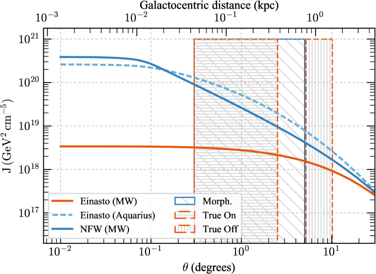
Figure 1: J factor as a function of angular distance from the GC for the two profiles considered in this work (derived from a fit to the rotation curve of the Milky Way Pato et al. (2015)) with those parameters in the text (Sec. II.1): NFW (solid blue line) and Einasto (solid orange). For comparison, we also show as a dashed blue line the J factor given by the Einasto profile used in Refs. Silverwood et al. (2015); Abdallah et al. (2016b); Carr et al. (2016). For each value of $\theta$ the integral over the solid angle in Eq. (1) is evaluated over an azimuthal angle interval of $0.1^{\circ}$. Regions of the GC halo that will be used in our analysis are also depicted in the figure as striped areas delimited by vertical lines (see legend). These regions depend on the observational strategy adopted in each case, see Sec. IV.1 for full details.

We note that other parameter choices have been made for the DM density profiles in previous work. For instance, the authors of Ref. Silverwood et al. (2015) use an Einasto profile with $\rho_{local}=0.4\,\mathrm{GeV}\,\mathrm{cm}^{-3}$ at $r_{\odot}=8.5\,$kpc, $\alpha=0.17$, and $r_{s}=20\,$kpc. The same values were also adopted in the recent analysis of the GC halo by the H.E.S.S. Collaboration Abdallah et al. (2016b), and are partially motivated by the results of the Aquarius $N$-body simulations Springel et al. (2008); Pieri et al. (2011).

With these parameters at hand we use the CLUMPY code Charbonnier et al. (2012); Bonnivard et al. (2016) to calculate the J factor for both NFW and Einasto profiles with the parameters given above. More specifically, CLUMPY provides all-sky J factor maps for each DM profile in Galactic coordinates. The resulting J factors as a function of angular distance from the GC can be seen in Fig. 1. For the sake of comparison, we also show in the same figure the J factor given by the Einasto profile used in Refs. Silverwood et al. (2015); Abdallah et al. (2016b); Carr et al. (2016). Note that the latter profile yields a J factor which is indeed more similar to the one obtained with our NFW profile rather than with the Einasto profile we use.

Finally, we note that only the smooth DM component of the Galaxy has been included in either case, as any possible enhancement due to halo substructure is expected to be very marginal in the inner Galactic regions, where these analyses are performed Sanchez-Conde et al. (2011); Palomares-Ruiz and Siegal-Gaskins (2010).

Having discussed the astrophysical inputs relevant for our reasoning we will describe the particle physics interactions we are probing. We start with the EFT framework.

II.2 Effective field theory

We examine four dimension-six benchmark operators describing Dirac fermion DM interacting with SM quarks via scalar, pseudoscalar, vector, and axial-vector interactions Goodman et al. (2010),

$$\mathcal{O}_{S} = \frac{m_{q}}{M_{\star}^{3}}(\bar{\chi}\chi)(\bar{q}q),$$ (4)

$$\mathcal{O}_{P} = \frac{m_{q}}{M_{\star}^{3}}(\bar{\chi}\gamma^{5}\chi)(\bar{q}\gamma^{5}q),$$ (5)

$$\mathcal{O}_{V} = \frac{1}{M_{\star}^{2}}(\bar{\chi}\gamma^{\mu}\chi)(\bar{q}\gamma_{\mu}q),$$ (6)

$$\mathcal{O}_{A} = \frac{1}{M_{\star}^{2}}(\bar{\chi}\gamma^{\mu}\gamma^{5}\chi)(\bar{q}\gamma_{\mu}\gamma^{5}q).$$ (7)

Here $M_{\star}$ is the energy scale describing the strength of the interaction, and $\gamma_{\mu},\,\gamma_{5}$ are the standard Dirac gamma matrices. These operators were chosen since they display various types of suppression of the annihilation and scattering rate, summarized in Table 1. The annihilation rate is $p$-wave suppressed for operator $\mathcal{O}_{S}$, and so is proportional to the DM velocity squared $v^{2}\sim 10^{-6}$. Operator $\mathcal{O}_{A}$ has a $p$-wave suppressed term, and a helicity-suppressed $s$-wave term proportional to $m_{q}^{2}$. Therefore we expect ID constraints to be relatively weaker for these operators. For operators $\mathcal{O}_{P}$ and $\mathcal{O}_{A}$, the scattering rates are either suppressed by the spin of the target nucleus $\vec{s}_{N}$ or the scattering momentum exchange $\vec{q}$ or both, rendering weak DD constraints. Operators $\mathcal{O}_{S}$ and $\mathcal{O}_{P}$ have interaction strengths suppressed by a Yukawa coupling in order to be consistent with the principle of minimal flavor violation D’Ambrosio et al. (2002); Goodman et al. (2010, 2011); Abdallah et al. (2015). This suppresses the ID rate especially when annihilation to top quarks is not kinematically accessible. It also leads to relatively weaker collider constraints. The operator $\mathcal{O}_{V}$ is unique amongst our choice of operators in that it has an unsuppressed rate for collider, DD and ID experiments. To ease comparison with collider constraints, we assume that the DM couples only to quarks, with an equal coupling to each generation; i.e. $M_{\star}$ is independent of flavor.

Table 1: Summary of the suppression effects the four operators lead to in indirect and direct detection of DM.

	ID	DD
$\mathcal{O}_{S}$	$v^{2}$	1
$\mathcal{O}_{P}$	1	$(\vec{s}_{\chi}\cdot\vec{q})\,(\vec{s}_{N}\cdot\vec{q})$
$\mathcal{O}_{V}$	1	1
$\mathcal{O}_{A}$	$m_{q}^{2}$, $v^{2}$	$\vec{s}_{\chi}\cdot\vec{s}_{N}$

We use the PPPC4DMID code Cirelli et al. (2011); Ciafaloni et al. (2011) to determine the spectrum of photons induced by annihilation into quarks. This is the spectrum at source, and includes the effects of electroweak radiative corrections but neglects secondary photons produced during propagation to Earth such as from inverse Compton scattering and synchrotron emission. The branching ratios and the conversion between limits on $\langle\sigma v\rangle$ and $M_{\star}$ are given by the DM annihilation rates for each operator,

$$\langle\sigma v\rangle_{\mathcal{O}_{S}} = \sum_{q}\Theta(m_{\chi}-m_{q})\frac{m_{q}^{2}}{M_{\star}^{6}}\frac{3m_{\chi}^{2}}{8\pi}\left(1-\frac{m_{q}^{2}}{m_{\chi}^{2}}\right)^{3/2}v^{2},$$ (8)

$$\langle\sigma v\rangle_{\mathcal{O}_{P}} = \sum_{q}\Theta(m_{\chi}-m_{q})\frac{m_{q}^{2}}{M_{\star}^{6}}\frac{3m_{\chi}^{2}}{16\pi}\sqrt{1-\frac{m_{q}^{2}}{m_{\chi}^{2}}}$$ (9)

$$\times\left(8+\frac{2-m_{q}^{2}/m_{\chi}^{2}}{1-m_{q}^{2}/m_{\chi}^{2}}v^{2}\right),$$

$$\langle\sigma v\rangle_{\mathcal{O}_{V}} = \sum_{q}\Theta(m_{\chi}-m_{q})\frac{1}{M_{\star}^{4}}\frac{m_{\chi}^{2}}{2\pi}\sqrt{1-\frac{m_{q}^{2}}{m_{\chi}^{2}}}$$

$$\times\left(6+3\frac{m_{q}^{2}}{m_{\chi}^{2}}+\frac{8-4{m_{q}^{2}}/{m_{\chi}^{2}}+5{m_{q}^{4}}/{m_{\chi}^{4}}}{8\left(1-{m_{q}^{2}}/{m_{\chi}^{2}}\right)}v^{2}\right),$$

$$\langle\sigma v\rangle_{\mathcal{O}_{A}} = \sum_{q}\Theta(m_{\chi}-m_{q})\frac{1}{M_{\star}^{4}}\frac{m_{\chi}^{2}}{4\pi}\sqrt{1-\frac{m_{q}^{2}}{m_{\chi}^{2}}}$$

$$\times\left(6\frac{m_{q}^{2}}{m_{\chi}^{2}}+\frac{8-22{m_{q}^{2}}/{m_{\chi}^{2}}+17{m_{q}^{4}}/{m_{\chi}^{4}}}{4\left(1-{m_{q}^{2}}/{m_{\chi}^{2}}\right)}v^{2}\right),$$

where $\Theta$ is the Heaviside function, enforcing that DM can only annihilate to kinematically accessible states. Using the Heavyside function implies that we only take on-shell two-body final states into account. Allowing off-shell production would smooth the step functions and could significantly change the branching ratios near the threshold. The resultant spectra are shown in Fig. 2. For all operators but $\mathcal{O}_{V}$, one can see a jump in the hardness in the annihilation spectra where annihilation into $t\bar{t}$ quarks is kinematically accessible. It arises because these three models have leading terms in the annihilation proportional to the quark mass. For the same reason, the spectra for these operators and DM masses are very similar when represented as $dN/dx$ versus $x$, where $x=E/m_{\chi}$.

PPPC4DMID accounts for electroweak corrections up to next-to-leading-order (NLO) level. For annihilation into quarks this is done through the results of Ref. Ciafaloni et al. (2011). The NLO approximation breaks down for DM masses beyond 10 TeV and therefore we will not present limits on the EFT scale for larger values of $m_{\chi}$.

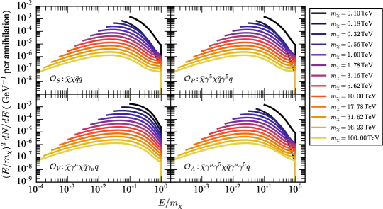
Figure 2: Average photon spectrum per DM annihilation into quarks. Photon spectra are from PPPC4DMID Cirelli et al. (2011); Ciafaloni et al. (2011) and branching ratios are determined using Eqs. (8)–(LABEL:sigvOA).

As aforementioned the EFT breaks down in some regimes, and for this reason, simplified models have become powerful tools to explore DM models, as we discuss below.

II.3 Simplified models

In order to aid in comparison with constraints from other experiments, we study four models recommended by the LHC Dark Matter Working Group (DMWG) Busoni et al. (2016), with Dirac fermion DM interacting with SM quarks via $s$-channel exchange of a scalar, pseudoscalar, vector, or axial-vector mediator (referred to as the $S$, $P$, $V$, and $A$ models in the following). They correspond to the simplest realization of the four effective operators we consider, and again nicely demonstrate the different classes of suppression. These models are described in detail in Ref. Busoni et al. (2016), and have interaction Lagrangians

$$\mathcal{L}_{S} = -g_{\chi}\phi\bar{\chi}\chi-\sum_{q}g_{q}\phi\frac{m_{q}}{m_{f}}\bar{q}q,$$ (12)

$$\mathcal{L}_{P} = -ig_{\chi}\phi\bar{\chi}\gamma_{5}\chi-\sum_{q}ig_{q}\phi\frac{m_{q}}{m_{f}}\bar{q}\gamma_{5}q,$$ (13)

$$\mathcal{L}_{V} = -g_{\chi}Z^{\prime}_{\mu}\bar{\chi}\gamma^{\mu}\chi-\sum_{q}g_{q}Z^{\prime}_{\mu}\bar{q}\gamma^{\mu}q,$$ (14)

$$\mathcal{L}_{A} = -g_{\chi}Z^{\prime}_{\mu}\bar{\chi}\gamma^{\mu}\gamma_{5}\chi-\sum_{q}g_{q}Z^{\prime}_{\mu}\bar{q}\gamma^{\mu}\gamma_{5}q,$$ (15)

where $m_{f}\simeq 246$ GeV is the Higgs vacuum expectation value, the factor of $m_{q}/m_{f}$ comes from a Yukawa coupling, and we assume $g_{q}$ is the same for all quarks. We follow the DMWG benchmark coupling strengths of $g_{q}=g_{\chi}=1$ for the $S$ and $P$ models, $g_{q}=0.25$, $g_{\chi}=1$ for the $V$ and $A$ models, and present exclusion contours in the $M_{\rm med}$-$m_{\chi}$ plane.

When kinematically accessible, each of these mediators has a decay width into fermions (quarks or DM) given by

$$\Gamma_{S}^{f\bar{f}} = c_{f}^{SP}\frac{g_{f}^{2}M_{\rm med}}{8\pi}\left(1-\frac{4m_{f}^{2}}{M_{\rm med}^{2}}\right)^{3/2},$$ (16)

$$\Gamma_{P}^{f\bar{f}} = c_{f}^{SP}\frac{g_{f}^{2}M_{\rm med}}{8\pi}\sqrt{1-\frac{4m_{f}^{2}}{M_{\rm med}^{2}}},$$ (17)

$$\Gamma_{V}^{f\bar{f}} = c_{f}^{VA}\frac{g_{f}^{2}M_{\rm med}}{12\pi}\sqrt{1-\frac{4m_{f}^{2}}{M_{\rm med}^{2}}}\left(1+\frac{2m_{f}^{2}}{M_{\rm med}^{2}}\right),$$ (18)

$$\Gamma_{A}^{f\bar{f}} = c_{f}^{VA}\frac{g_{f}^{2}M_{\rm med}}{12\pi}\left(1-\frac{4m_{f}^{2}}{M_{\rm med}^{2}}\right)^{3/2},$$ (19)

where $c_{\chi}^{SP}=c_{\chi}^{VA}=1$, $c_{q}^{SP}=3m_{q}^{2}/m_{f}^{2}$, and $c_{q}^{VA}=3$. In the $S,P$ models the mediator also decays to gluons,

$$\Gamma_{S}^{gg} = \frac{\alpha_{S}^{2}g_{q}^{2}M_{\rm med}^{3}\left|f_{\rm scalar}\left(\frac{4m_{t}^{2}}{M_{\rm med}^{2}}\right)\right|^{2}}{32\pi^{3}m_{f}^{2}},$$ (20)

$$\Gamma_{P}^{gg} = \frac{\alpha_{S}^{2}g_{q}^{2}M_{\rm med}^{3}\left|f_{\rm pseudoscalar}\left(\frac{4m_{t}^{2}}{M_{\rm med}^{2}}\right)\right|^{2}}{32\pi^{3}m_{f}^{2}},$$ (21)

where

$$f_{\rm scalar}(\tau)=\tau\left(1+(1-\tau)\tan^{-1}\left(\frac{1}{\sqrt{\tau-1}}\right)^{2}\right),$$ (22)

$$f_{\rm pseudoscalar}(\tau)=\tau\tan^{-1}\left(\frac{1}{\sqrt{\tau-1}}\right)^{2}.$$ (23)

The total minimum decay width is then

$$\Gamma_{S,\rm tot} = \Gamma_{S}^{gg}+\sum_{q}\Theta(M_{\rm med}-2m_{q})\Gamma_{S}^{q\bar{q}}$$ (24)

$$+\Theta(M_{\rm med}-2m_{\chi})\Gamma_{S}^{\chi\bar{\chi}},$$

$$\Gamma_{P,\rm tot} = \Gamma_{P}^{gg}+\sum_{q}\Theta(M_{\rm med}-2m_{q})\Gamma_{P}^{q\bar{q}}$$ (25)

$$+\Theta(M_{\rm med}-2m_{\chi})\Gamma_{P}^{\chi\bar{\chi}},$$

$$\Gamma_{V,\rm tot} = \sum_{q}\Theta(M_{\rm med}-2m_{q})\Gamma_{V}^{q\bar{q}}\Theta(M_{\rm med}-2m_{\chi})\Gamma_{V}^{\chi\bar{\chi}},$$

$$\Gamma_{A,\rm tot} = \sum_{q}\Theta(M_{\rm med}-2m_{q})\Gamma_{A}^{q\bar{q}}\Theta(M_{\rm med}-2m_{\chi})\Gamma_{A}^{\chi\bar{\chi}}$$

In principle the mediator could couple to other final states such as leptons, though we assume only the minimum width. These simplified models have similar DM annihilation rates to quarks as the effective operators described earlier,

$$\langle\sigma v\rangle_{S}^{q\bar{q}} = \frac{3g_{q}^{2}g_{\chi}^{2}}{8\pi}\frac{m_{q}^{2}}{m_{f}^{2}}\frac{m_{\chi}^{2}\left(1-\frac{m_{q}^{2}}{m_{\chi}^{2}}\right)^{3/2}}{\left(M_{\rm med}^{2}-4m_{\chi}^{2}\right)^{2}+\Gamma_{S,\rm tot}^{2}M_{\rm med}^{2}}v^{2},$$ (28)

$$\langle\sigma v\rangle_{P}^{q\bar{q}} = \frac{3g_{q}^{2}g_{\chi}^{2}}{2\pi}\frac{m_{q}^{2}}{m_{f}^{2}}\frac{m_{\chi}^{2}\sqrt{1-\frac{m_{q}^{2}}{m_{\chi}^{2}}}}{\left(M_{\rm med}^{2}-4m_{\chi}^{2}\right)^{2}+\Gamma_{P,\rm tot}^{2}M_{\rm med}^{2}},$$ (29)

$$+\mathcal{O}(v^{2})$$

$$\langle\sigma v\rangle_{V}^{q\bar{q}} = \frac{3g_{q}^{2}g_{\chi}^{2}}{2\pi}\frac{\left(m_{q}^{2}+2m_{\chi}^{2}\right)\sqrt{1-\frac{m_{q}^{2}}{m_{\chi}^{2}}}}{\left(M_{\rm med}^{2}-4m_{\chi}^{2}\right)^{2}+\Gamma_{V,\rm tot}^{2}M_{\rm med}^{2}}+\mathcal{O}(v^{2}),$$ (30)

$$\langle\sigma v\rangle_{A}^{q\bar{q}} = \frac{g_{q}^{2}g_{\chi}^{2}}{2\pi}$$ (31)

$$\times\frac{3m_{q}^{2}\left(1-\frac{4m_{\chi}^{2}}{M_{\rm med}^{2}}\right)^{2}\sqrt{1-\frac{m_{q}^{2}}{m_{\chi}^{2}}}+m_{\chi}^{2}v^{2}+\mathcal{O}(m_{q}^{2}v^{2})}{\left(M_{\rm med}^{2}-4m_{\chi}^{2}\right)^{2}+\Gamma_{A,\rm tot}^{2}M_{\rm med}^{2}}$$

$$+\mathcal{O}(v^{4}).$$

In the $S$ and $P$ models, DM can also annihilate to gluons via a quark loop. Across most of the parameter space this is subdominant to direct annihilation into quarks or the mediator, but can be important when the DM is light and annihilation to top quarks or mediators is not kinematically allowed, and is therefore included for completeness. The annihilation rate is given by

$$\langle\sigma v\rangle_{S}^{gg} = \frac{\alpha^{2}}{8\pi^{3}m_{f}^{2}}\frac{2g_{q}^{2}g_{\chi}^{2}m_{\chi}^{4}v^{2}}{\left(M_{\rm med}^{2}-4m_{\chi}^{2}\right)^{2}+\Gamma_{S,\rm tot}^{2}M_{\rm med}^{2}}$$ (32)

$$\times\left|\sum_{q}f_{\rm scalar}\left(\frac{m_{q}^{2}}{m_{\chi}^{2}}\right)\right|^{2},$$

$$\langle\sigma v\rangle_{P}^{gg} = \frac{\alpha^{2}}{2\pi^{3}m_{f}^{2}}\frac{g_{q}^{2}g_{\chi}^{2}}{\left(M_{\rm med}^{2}-4m_{\chi}^{2}\right)^{2}+\Gamma_{P,\rm tot}^{2}M_{\rm med}^{2}}$$ (33)

$$\times\left|\sum_{q}m_{q}^{2}f_{\rm pseudoscalar}\left(\frac{m_{q}^{2}}{m_{\chi}^{2}}\right)\right|^{2}.$$

When the DM mass is heavier than the mediator mass, direct annihilation to the mediator becomes accessible, with the mediator subsequently decaying into SM particles. The annihilation rates are

$$\langle\sigma v\rangle_{S}^{SS} = \frac{g_{\chi}^{4}m_{\chi}v^{2}}{24\pi}$$

$$\times\frac{\left(9m_{\chi}^{6}-17M_{\rm med}^{2}m_{\chi}^{4}+10M_{\rm med}^{4}m_{\chi}^{2}-2M_{\rm med}^{6}\right)}{\sqrt{m_{\chi}^{2}-M_{\rm med}^{2}}\left(2m_{\chi}^{2}-M_{\rm med}^{2}\right)^{4}},$$

$$\langle\sigma v\rangle_{P}^{PP} = \frac{g_{\chi}^{4}m_{\chi}\left(m_{\chi}^{2}-M_{\rm med}^{2}\right)^{5/2}}{24\pi\left(2m_{\chi}^{2}-M_{\rm med}^{2}\right)^{4}}v^{2},$$ (35)

$$\langle\sigma v\rangle_{V}^{VV} = \frac{g_{\chi}^{4}\left(m_{\chi}^{2}-M_{\rm med}^{2}\right)^{3/2}}{4\pi m_{\chi}\left(M_{\rm med}^{2}-2m_{\chi}^{2}\right)^{2}}+\mathcal{O}(v^{2}),$$ (36)

$$\langle\sigma v\rangle_{A}^{AA} = \frac{g_{\chi}^{4}\left(m_{\chi}^{2}-M_{\rm med}^{2}\right)^{3/2}}{4\pi m_{\chi}\left(M_{\rm med}^{2}-2m_{\chi}^{2}\right)^{2}}+\mathcal{O}(v^{2}).$$ (37)

The total annihilation cross sections are then:

$$\langle\sigma v\rangle_{S}^{\mathrm{total}} = \langle\sigma v\rangle_{S}^{gg}+\Theta(m_{\chi}-M_{\rm med})\langle\sigma v\rangle_{S}^{SS}$$ (38)

$$+\sum_{q}\Theta(m_{\chi}-m_{q})\langle\sigma v\rangle_{S}^{q\bar{q}},$$

$$\langle\sigma v\rangle_{P}^{\mathrm{total}} = \langle\sigma v\rangle_{P}^{gg}+\Theta(m_{\chi}-M_{\rm med})\langle\sigma v\rangle_{P}^{PP}$$ (39)

$$+\sum_{q}\Theta(m_{\chi}-m_{q})\langle\sigma v\rangle_{P}^{q\bar{q}},$$

$$\langle\sigma v\rangle_{V}^{\mathrm{total}} = \Theta(m_{\chi}-M_{\rm med})\langle\sigma v\rangle_{V}^{VV}$$ (40)

$$+\sum_{q}\Theta(m_{\chi}-m_{q})\langle\sigma v\rangle_{V}^{q\bar{q}},$$

$$\langle\sigma v\rangle_{A}^{\mathrm{total}} = \Theta(m_{\chi}-M_{\rm med})\langle\sigma v\rangle_{A}^{AA}$$ (41)

$$+\sum_{q}\Theta(m_{\chi}-m_{q})\langle\sigma v\rangle_{A}^{q\bar{q}}.$$

The branching ratios to various final states are shown in Fig. 3 for the $S$ and $V$ models. For the $A$ model, annihilation to the heaviest kinematically accessible quark dominates. For the $P$ model, annihilation to top quarks dominates when kinematically accessible. Below this threshold, gluons are the leading annihilation channel.

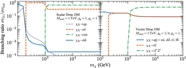
Figure 3: Branching ratios for the $S$ and $V$ models for $g_{q}=g_{\chi}=1$ ($S$) and $g_{q}=0.25,g_{\chi}=1$ ($V$), with $M_{\mathrm{med}}=1\,$TeV.

The photon spectra per DM annihilation to quarks and gluons are again determined using PPPC4DMID. The photon spectrum per annihilation into mediators is a little more involved. The spectrum from the decay of a mediator into quarks and gluons is calculated using PPPC4DMID in the mediator rest frame as usual, with branching ratios from Eqs. (16)–(21). These spectra are then Lorentz boosted into the DM center-of-mass frame using the procedure from Ref. Bergstrom et al. (2009); Elor et al. (2015). For each model, the spectra from annihilation to quarks, gluons and mediators are combined and weighted by their respective branching ratios using Eqs. (28)–(37). Results are shown in Fig. 4. The spectra are very similar to the EFT case, in the sense that jumps in the spectral hardness are observed once annihilation into $t\bar{t}$ becomes kinematically possible for the $S$, $P$, and $A$ models. In this figure we can also see the resonant enhancement of the annihilation rate around the region $M_{\rm med}\simeq 2m_{\chi}$.

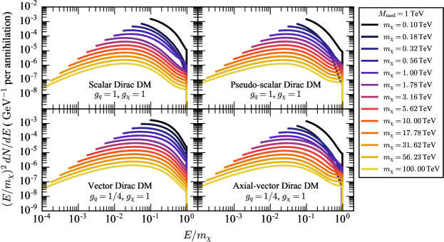
Figure 4: Simplified model PPPC4DMID spectra for $M_{\mathrm{med}}=1\,$TeV

After discussing the important ingredients for the determination of the expected $\gamma$-ray signal from DM annihilation, we describe the procedure used to assess CTA sensitivity and the expected $\gamma$-ray backgrounds.

III Expected Backgrounds

For IACTs the major source of background is cosmic rays (CRs), which consist mainly of protons but also heavier nuclei, as well as electrons and positrons. The flux of CRs is in general by a factor of $10^{3}$ larger than $\gamma$-ray signals from point sources, requiring efficient techniques to reject showers initiated by CRs (see e.g. Ref. Völk and Bernlöhr (2009)). This can be achieved by means of the shower image, and potentially the arrival time of the shower front Aharonian et al. (2008). However, a residual contamination of the $\gamma$-ray sample with CRs is inevitable. The expected CR background for CTA has been derived through extensive Monte Carlo simulations taking into account the different possible array layouts Bernlöhr et al. (2013). Here, we use the so-called prod 2 version of these background simulations to derive the expected number of CR background events. Due to the soft CR spectrum (see e.g. Ref. Patrignani et al. (2016) for a review), this background component will be especially important at low energies, but we expect it to dominate over the entire energy range in comparison to a DM signal with an annihilation cross section yielding the expected DM relic abundance, $\langle\sigma v\rangle\sim 3\times 10^{-26}\,\mathrm{cm}^{3}\,\mathrm{s}^{-1}$.

An additional source of background is astrophysical Galactic diffuse emission (GDE) caused by the interaction of CR with interstellar dust and radiation fields. Below 100 GeV, the GDE has been measured with the Fermi LAT and found to be dominated by $\pi^{0}$ decay, inverse Compton scattering, as well as bremsstrahlung, and the first two contributions dominate for energies above a few GeV Ackermann et al. (2012). At energies between 0.2 and 20 TeV, diffuse $\gamma$-ray emission has been detected with H.E.S.S. from the GC ridge for Galactic latitudes $|b|<0.3^{\circ}$ and $|l|<0.8^{\circ}$ Aharonian et al. (2006b). The authors of Ref. Silverwood et al. (2015) found that neglecting GDE leads to a strong overestimation of the differential sensitivity for the DM signal from the GC. We therefore follow Ref. Silverwood et al. (2015) and estimate the background contribution of the GDE with the template provided by the Fermi-LAT Collaboration. We use a simple power-law extrapolation of the template for $\gamma$-ray energies above 100 GeV. This yields a conservative estimate of the GDE at higher energies as a potential cutoff in the GDE energy spectrum would yield less background counts. In comparison to Ref. Aharonian et al. (2006b), the extrapolation overestimates the diffuse flux in the same sky region by approximately 2 orders of magnitude. For the GDE measurement with Milagro at a median energy of 15 TeV for latitudes $-2^{\circ}<b<2^{\circ}$ and longitudes $30^{\circ}<l<65^{\circ}$ and $65^{\circ}<l<85^{\circ}$ Abdo et al. (2008) the extrapolation overpredicts the flux by more than 4 orders of magnitude.

We neglect any contribution from resolved and unresolved point sources. One known source in the region is HESS 1745-303. In a real analysis the source can be simply cut out as done in H.E.S.S. analyses (see e.g. Fig. 1 of the Supplemental Material of Ref. Abdallah et al. (2016a)). A similar approach could be taken for additional sources identified in the Galactic plane survey which will be conducted with CTA. Evidence for unresolved sources like millisecond pulsars has been recently found and such a population could explain the $\gamma$-ray excess observed in the Galactic center Lee et al. (2016); Bartels et al. (2016); Ajello et al. (2017). If these sources are indeed millisecond pulsars, they should not contribute in the CTA energy range as their spectra usually lexhibit cutoffs at a few tens of GeV.

IV Analysis framework

We use ctools version 1.0.1 Knödlseder et al. (2016) to calculate sky maps with the expected number of counts from GDE, CR background, and a potential DM signal. The ctools package folds the predicted intensity for the diffuse DM signal and the GDE with the CTA instrumental response functions (IRFs), taking into account the point spread function (PSF), which relates the true arrival direction of the $\gamma$ ray $\mathbf{p}$ to the reconstructed direction $\mathbf{p}^{\prime}$, effective area $A_{\mathrm{eff}}$, and the energy-dependent size of the field of view (FOV). We neglect the energy dispersion, which should not have a large effect since all spectral components are smooth and do not show narrow features. The prod 2 Monte Carlo CR background templates for the southern CTA baseline array Bernlöhr et al. (2013) are implemented through the CTA IRF background model. Within ctools, the PSF, effective area, and background intensity are extrapolated using analytical expressions in order to calculate the off-axis performance. We calculate the sky maps within six logarithmic energy bins per decade in an energy range from 30 GeV to 100 TeV and use a pixelization of $0.0625^{\circ}\,\mathrm{pixel}^{-1}$.

IV.1 Observational strategy

Within the first three years of CTA operations it is planned to conduct a survey of the central Galaxy to achieve a uniform exposure within a $2^{\circ}$ radius around the GC Carr et al. (2016). As the final layout of the pointing scheme is not yet known, we will assume a pointing centered on the GC and compute the expected number of counts within $10^{\circ}\times 10^{\circ}$ sky maps. We will refer to this region as FOV. One should keep in mind that the FOV is energy dependent. At low energies, mostly the large-size telescopes will contribute to the sensitivity which have a field of view of about $4.5^{\circ}$. At the highest energies, the small sized-telescopes contribute most and have a FOV of $\sim 9^{\circ}$. Therefore, we do not expect any counts at large angular distances from the FOV center at low energies.

DM searches with IACTs are usually performed by dividing the FOV into multiple regions of interest (RoIs), where regions with a large expected DM signal are referred to as “on” regions whereas regions with negligible DM contribution are referred to as “off” regions. The off regions provide an estimate for the expected number of background events. The sensitivity can be increased by using multiple on and off regions in order to probe the different spatial morphology of the background and DM signal (e.g. Silverwood et al. (2015); Lefranc et al. (2015); Abdallah et al. (2016b)).

For our assumed NFW profile, we follow Refs. Lefranc et al. (2015); Carr et al. (2016) and divide the FOV into five concentric rings with a width of $1^{\circ}$. The outermost ring has an outer radius of $5^{\circ}$ (see the upper panels of Fig. 5). We do not use a separate off region but rather model the contributions from all sources simultaneously Silverwood et al. (2015). For our assumed Einasto DM density profile, the FOV will be too small to achieve a sufficient contrast between the DM signal and the background with this setup. For this profile, we therefore assume “true” on/off observations with three independent pointings as conducted by the H.E.S.S. Collaboration Abramowski et al. (2015). We use three $5^{\circ}\times 5^{\circ}$ RoIs, with the central one centered on $(l,b)=(1^{\circ},-0.7^{\circ})$ and the other two shifted by $\pm 35^{\prime}$ in right ascension (corresponding to an angular separation of $\sim 7.66^{\circ}$ between the RoI centers). The RoIs are shown in the lower panels of Fig. 5. By consecutively observing the on and off regions, differences in azimuth and zenith angle distributions are minimized. For all pointing strategies we exclude Galactic latitudes $|b|<0.3^{\circ}$ to minimize contamination from GDE. We stress that we do not attempt to optimize the observational strategy to find the optimal spectral and spatial binning. In principle, these should be optimized for different DM density profiles, DM spectra, and observation energy (due to the energy dependent FOV). This is, however, beyond the scope of this study.

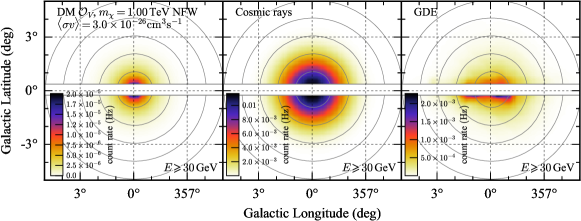
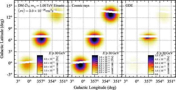
Figure 5: Adopted pointing schemes. From left to right the panels show the expected count rate for the different model components included here (DM, CR, and GDE). For the DM, we show the expected rate for the $\mathcal{O}_{V}$ operator and $m_{\chi}=1\,$TeV with $\langle\sigma v\rangle=3\times 10^{-26}\,\mathrm{cm}^{3}\mathrm{s}^{-1}$. Top: Pointing schemes for the morphological analysis adopted for the NFW profile. Bottom: True on/off pointings for the Einasto profile.

IV.2 Likelihood analysis

We use a binned Poisson likelihood analysis to derive the CTA sensitivity and closely follow the methodology outlined in Ref. Silverwood et al. (2015), i.e. we do not estimate the background events from independent off regions. Instead, we use templates for all model components in all spatial bins and fit each contribution (DM, CR, GDE) simultaneously. For the chosen observational strategies we use ctools to calculate the expected number of counts $\mu_{ik}^{\mathrm{X}}$ for contribution X$=$DM, GDE, CR, for each energy bin $i$ and pixel $k$ within solid angle $\Omega_{k}$ [see Eq. (4) in Ref. Knödlseder et al. (2016)],

$$\mu_{ik}^{\mathrm{X}} = \mathrm{T}_{\mathrm{obs}}\,\int\limits_{\Omega_{k}}d\Omega\int\limits_{\Delta E_{i}}dE\int\limits_{\mathbf{p}}d\mathbf{p}\,A_{\mathrm{eff}}(\mathbf{p},E)$$ (42)

$$\times\mathrm{PSF}(\mathbf{p}^{\prime}|\mathbf{p},E)\frac{\mathrm{d}N^{\mathrm{X}}}{\mathrm{d}E}(E,\mathbf{p}),$$

where $\mathrm{T}_{\mathrm{obs}}$ is the observation time, $\mathbf{p},\mathbf{p}^{\prime}$ are the true and reconstructed $\gamma$-ray arrival directions, respectively, and $dN^{\mathrm{X}}/dE$ is the diffuse model for $\gamma$-ray emission from component X. The expected counts for all pixels and model components above 30 GeV are shown in Fig. 5. The number of expected counts in RoI $j$ is then simply $\mu_{ij}^{X}=\sum_{k\in\mathrm{RoI}_{j}}\mu_{ik}^{X}$ for all pixel $k$ in RoI $j$. An example of the resulting count rate spectrum for the innermost ring of the pointing strategy adopted for the NFW profile is shown in Fig. 6 (top). With our chosen extrapolation of the GDE above 100 GeV, it dominates the count rate above $\sim 10\,$TeV. The count rate in each ring integrated above 30 GeV is shown in Fig. 6 (bottom). For a constant acceptance, one would expect the CR to increase for the RoIs with larger distances to the GC due to the increasing solid angle. This is not the case here due to decreasing exposure towards the edges of the FOV.

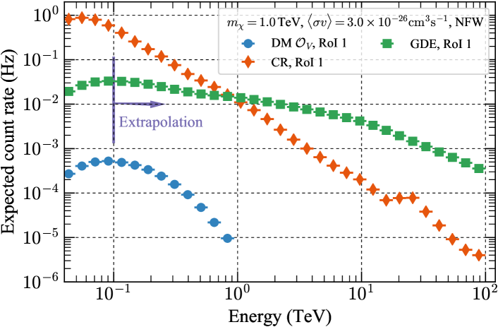
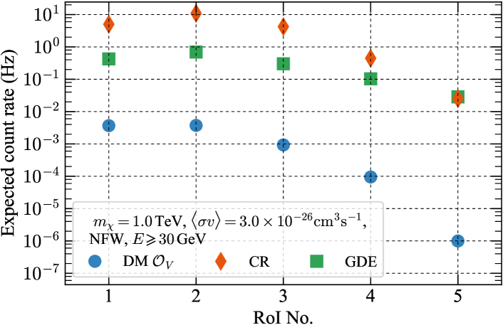
Figure 6: Expected count rates for the different source components for the NFW profile and morphological pointing strategy. The DM component is shown for the $\mathcal{O}_{V}$ operator and $m_{\chi}=1\,$TeV with $\langle\sigma v\rangle=3\times 10^{-26}\,\mathrm{cm}^{3}\mathrm{s}^{-1}$. Top: Expected count rate as a function of energy for the innermost RoI. The energy above which the GDE is extrapolated is marked by a blue arrow. Bottom: Count rate for each RoI integrated above 30 GeV.

The total number of expected counts for each energy and RoI is given by the sum of the model components:

$$\mu_{ij}=\mu^{\mathrm{DM}}_{ij}+R^{\mathrm{CR}}_{i}\mu^{\mathrm{CR}}_{ij}+R^{\mathrm{GDE}}_{i}\mu^{\mathrm{GDE}}_{ij}.$$ (43)

In the statistical analysis, we allow each component to be rescaled independently in each energy bin. For the DM component this is done by changing $\langle\sigma v\rangle$ while the parameters $R_{i}^{\mathrm{CR,GDE}}$ change each background contribution. Up to a constant, the likelihood for $\mathbf{n}$ observed number of counts is given by

$$\ln\mathcal{L}(\boldsymbol{\mu},\boldsymbol{\theta}|\mathbf{n})=\sum\limits_{i,j}\left[n_{ij}\ln\left(\alpha_{ij}\mu_{ij}\right)-\alpha_{ij}\mu_{ij}-\frac{(1-\alpha_{ij})^{2}}{2\sigma_{\alpha}^{2}}\right],$$ (44)

where we introduced the terms $\alpha_{ij}$ that allow us to account for systematic uncertainties such as an unmodeled variation in the exposure between the different RoIs. Each $\alpha_{ij}$ is assumed to follow a Gaussian likelihood with a width of $\sigma_{\alpha}=0.01$ Silverwood et al. (2015). The nuisance parameters are given by $\boldsymbol{\theta}=(\mathbf{R}^{\mathrm{GDE}},\mathbf{R}^{\mathrm{CR}},\boldsymbol{\alpha})$.

Instead of simulating a large set of different Poisson realizations of the observed counts, we use the “Asimov data set”; i.e. we set the observed counts equal to the number of expected counts, $n_{ij}=\mu_{ij}$ Cowan et al. (2011). We do not assume any contribution from DM and set $\mu_{ij}^{\mathrm{DM}}=0$ and $R_{i}^{\mathrm{GDE}}=R_{i}^{\mathrm{CR}}=1$. For each tested DM operator and mass, we step through $\langle\sigma v\rangle$ and calculate the test statistic

$$\lambda(m_{\chi},\langle\sigma v\rangle)=-2\ln\left(\frac{\mathcal{L}(\boldsymbol{\mu}(m_{\chi},\langle\sigma v\rangle),\widehat{\widehat{{\boldsymbol{\theta}}}}(m_{\chi},\langle\sigma v\rangle)|\mathbf{n})}{\mathcal{L}(\widehat{\boldsymbol{\mu}},\widehat{\boldsymbol{\theta}}|\mathbf{n})}\right),$$ (45)

where $\widehat{\widehat{\boldsymbol{\theta}}}(m_{\chi},\langle\sigma v\rangle)$ are the nuisance parameters that maximize $\mathcal{L}$ for a given set of $m_{\chi},\langle\sigma v\rangle$, and $\widehat{\boldsymbol{\mu}}$ and $\widehat{\boldsymbol{\theta}}$ denote the unconditional maximum likelihood estimators. For the simplified models, $\boldsymbol{\mu}$ and $\widehat{\widehat{\boldsymbol{\theta}}}$ (and consequently $\lambda$) additionally depend on $M_{\mathrm{med}}$. For each DM operator and mass we then set 95 % confidence limits on the annihilation cross section that results in $\lambda=2.71$. Following Ref. Silverwood et al. (2015), we restrict $0.5\leqslant R_{i}^{\mathrm{CR}}\leqslant 1.5$ and furthermore $0.2\leqslant R_{i}^{\mathrm{GDE}}\leqslant 5$.

V Results

Before comparing the potential limits on the annihilation cross section in the EFT and simplified model frameworks to DD and LHC results, we compare our results for an annihilation of Majorana DM [$x=1$ in Eq. (1)] into $b\bar{b}$ quarks with the results of previous CTA sensitivity estimates Silverwood et al. (2015); Lefranc et al. (2015); Carr et al. (2016) (Fig. 7). We assume a 100 hour observation in the case of the morphological analysis, and 100 hours for each RoI in the case of the true on/off observations. The limits for our assumed Einasto profile are an order of magnitude weaker than those assuming the NFW profile despite the larger observation time, due to the lower J factor (see Fig. 1). For simplicity, we only show curves from other works that neglect systematic uncertainties and the GDE. This is also the main reason why, for the NFW profile we consider, our projected limits are worse by more than 1 order of magnitude. If we also neglect both the effects of systematic uncertainties and the GDE, our limits improve by a factor of $\sim 12$ (blue dashed line in Fig. 7). In addition, if we use the DM density profile of Ref. Pieri et al. (2011), the limits improve by an overall factor of $\sim 20$ (light-blue dashed line in Fig. 7) compared to our fiducial setup and are, in this case, comparable to those of Ref. Carr et al. (2016). We also show the limits if we neglect systematic uncertainties but include GDE (dotted blue line) and if we neglect GDE but include systematic uncertainties (dotted-dashed blue line). Inclusion of GDE has a large effect at high DM masses, since we have chosen a simple power-law extrapolation of the Fermi-LAT GDE template which likely overestimates the GDE at high energies. Interestingly, the effect of systematic uncertainties dominates for $m_{\chi}\lesssim 300$ GeV in comparison to the GDE. The reason is the following for low mass DM; only the first energy bins contribute to the likelihood due to the cutoff of the DM annihilation $\gamma$-ray spectrum. Furthermore, due to the smaller FOV of CTA at low energies, only the innermost spatial rings contribute. Yet, for these energy bins, the expected DM flux (for fixed $\langle\sigma v\rangle$) in each energy bin will be higher for a low mass DM particle compared to a high mass one since the DM flux is suppressed with $m_{\chi}^{2}$. In the likelihood fit, the relatively high expected DM flux for low masses can be compensated with the systematic uncertainty term (cf. Eq. (44)). For high DM masses, the expected DM flux in each energy bin is small and hence the systematic uncertainty term has a smaller effect on the fit. However, more energy bins contribute to the the overall likelihood. Moreover, more spatial bins are included in the fit, further reducing the effect of systematic uncertainties.

We conclude that our analysis – compared to previous analyses – yields conservative results for the CTA sensitivity to the detection of DM due to the inclusion of systematic uncertainties, the GDE modeled without a high energy cutoff, and the lower J factor. We furthermore have not optimized the analysis in terms of the spatial or spectral binning which will be done in a forthcoming publication of the CTA consortium.

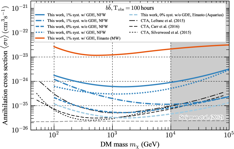
Figure 7: Upper limits on the cross section for 100 % annihilation of Majorana DM into $b\bar{b}$ for our fiducial analysis (1 % systematic uncertainty, including GDE) for the two assumed DM density profiles (blue solid line, NFW; orange solid line, Einasto). For comparison we also show our limits for 0 % systematic uncertainty for the NFW profile with and without GDE (blue dotted and dashed line, respectively) and for the Einasto profile of the Aquarius simulation (light-blue dashed line). The blue dashed-dotted line shows the limits without GDE but 1 % systematic uncertainty. We compare our limits to previous results for the same observation time but not including systematic uncertainties and GDE Silverwood et al. (2015); Lefranc et al. (2015); Carr et al. (2016). The annihilation cross section resulting in the right relic density is shown as a gray dashed line using the result from Ref. Steigman et al. (2012) (and an extrapolation thereof to 100 TeV). The NLO approximation of PPPC4DMID breaks down for $m_{\chi}>10\,$TeV, indicated by the gray shaded region.

V.1 Effective field theory

For each of the EFT operators listed in Sec. II.2, we derive upper limits on the cross section in the same way as with the pure annihilation into $b\bar{b}$ above. The results are shown in Fig. 8. The assumed observation times are the same as before. Remarkably, the limits are very similar for the $\mathcal{O}_{S,P,A}$ operators and are slightly better for the vector operator $\mathcal{O}_{V}$. This weak dependence on the exact operator demonstrates that limits from other operators not included in the present analysis should not yield very different results. As for the $b\bar{b}$ case, the limits degrade by an order of magnitude if the DM follows the Einasto profile (orange lines) instead of the NFW (blue lines). The weakening of the $\mathcal{O}_{S,P,A}$ limits at 180 GeV appears when annihilation into top quarks becomes kinematically available and will be further discussed in the simplified model case below.

The limits on $\langle\sigma v\rangle$ can then be transformed into lower limits on the EFT scale $M_{\star}$ using Eqs. (8)-(LABEL:sigvOA). The constraints for our NFW and Einasto profiles are shown in Fig. 9 as dark-red and red shaded regions, respectively, together with bounds from DD experiments (green lines) and the LHC (dark-purple shaded region). Due to the strong dependence of $\langle\sigma v\rangle$ on $M_{\star}$ ($\langle\sigma v\rangle\propto M_{\star}^{-6}$ for $\mathcal{O}_{S,P}$ and $\langle\sigma v\rangle\propto M_{\star}^{-4}$ for $\mathcal{O}_{V,A}$), the lower limits do not depend strongly on the assumed DM density profile in contrast to the limits on the annihilation cross section.

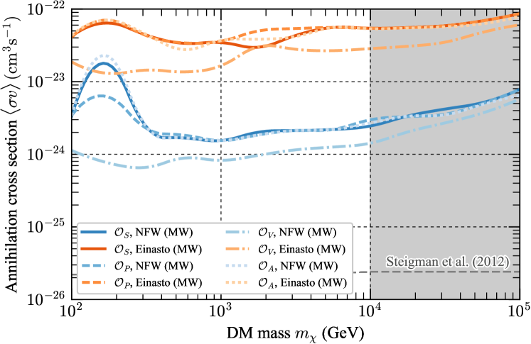
Figure 8: Limits on the annihilation cross section for the different EFT operators and DM density profiles. The NLO approximation of PPPC4DMID breaks down for $m_{\chi}>10\,$TeV, indicated by the gray shaded region.

In general, the lower limits for CTA follow the expectations for the suppression of indirect detection of the operators listed in Table 1. The strongest limits are found for the vector and pseudoscalar operators, $\mathcal{O}_{V}$ and $\mathcal{O}_{P}$, respectively. Only for the pseudoscalar operator, CTA might be able to probe the cross section resulting in the correct thermal DM relic abundance and the corresponding values for $M_{\star}$. These are given by the gray band in Fig. 9. The band is derived from the standard equation Gelmini et al. (1991),

$$\Omega_{\chi}h^{2}=\frac{1.07\times 10^{9}\,\mathrm{GeV}^{-1}}{M_{\mathrm{Pl}}}\frac{x_{F}}{\sqrt{g_{*}}}\frac{1}{a+3b/x_{F}},$$ (46)

where $M_{\mathrm{Pl}}\approx 1.22\times 10^{19}\,\mathrm{GeV}$ is the Planck mass, $h$ is Hubble parameter, $g_{*}$ is the number of relativistic degrees of freedom, and $x_{F}=m_{\chi}/T_{F}$ is the inverse freeze-out temperature scaled with WIMP mass. Following Ref. Blumenthal et al. (2015) we take $20<x_{F}<30$ Jungman et al. (1996); Cao et al. (2011) and $80<g_{*}<100$ Coleman and Roos (2003). We emphasize that these choices are rather simplistic but are sufficient in the context of the EFT to estimate the relic density curves. A more accurate description is required once we get closer to more concrete model building realizations as done in the simplified dark matter model section that we will discuss below. In any case, the coefficients $a$ and $b$ stem from the expansion of the cross section, $\langle\sigma v\rangle\sim a+bv^{2}$, and can be read off directly from Eqs. (8)-(LABEL:sigvOA). Setting $\Omega_{\chi}h^{2}=0.1$ as derived from Planck measurements Ade et al. (2016), the gray band follows from inserting the expressions for $a$ and $b$ into Eq. (46) and solving for $M_{\star}$. The band reflects the assumed range of values for $x_{F}$ and $g_{*}$.

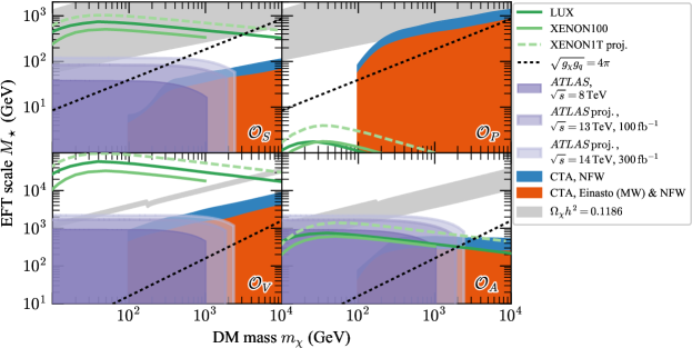
Figure 9: Lower limits on EFT scale $M_{\star}$ (red shaded regions) and comparison to LHC (purple shaded regions) and DD limits (green lines) for each tested EFT operator. Values of $M_{\star}$ and $m_{\chi}$ within the gray band result in the DM relic abundance as measured with Planck and the adopted range of values for $x_{F}$ and $g_{*}$. The EFT approximation is valid above the black dotted lines.

V.1.1 LHC comparison

For comparison we show LHC constraints on EFTs from Ref. Aad et al. (2015) (shown as a dark-purple shaded region in Fig. 9). EFT constraints at the LHC must be treated with caution, as the energy scale of the interaction may be large enough that the mediator is resolved, calling into question the validity of the EFT treatment. For recent reviews, see Refs. Abdallah et al. (2015); De Simone and Jacques (2016a); Kahlhoefer (2017). For the operators in question, the constraints are generally valid for effective coupling strengths of order unity or greater. Counterintuitively, the region of validity remains similar when moving from energy scales of 8 to 13 or 14 TeV, since the baseline constraint on $M_{\star}$ is strengthened at the same time as larger mediator masses become accessible ATL (2014). We use the Collider Reach tool col to rescale the constraints from Ref. Aad et al. (2015) and provide an approximate estimate of prospective reach at center-of-mass energy 13 TeV (14 TeV) and luminosity 100 fb${}^{-1}($300 fb^-1) as light-purple shaded regions in Fig. 9. These prospective limits should only be used as an indication, since the Collider Reach tool assumes that the details of the analysis are unchanged for the different center-of-mass energies and luminosities.

Regardless of the assumed DM density profile, it is clear that CTA will play a complementary role in the search for dark matter. Moreover, it will be possible to probe higher DM masses compared to the LHC, even considering prospects at 14 TeV and 300 fb^-1.

Above $m_{\chi}\sim 1\,$TeV the lower limits from CTA are always more constraining than the limits from the LHC. Especially for the vector and pseudoscalar operators CTA will be sensitive to DM annihilation signals out of reach of the LHC. The LHC should have a comparable sensitivity in the pseudoscalar case as in the scalar operator case Abercrombie et al. (2015).

V.1.2 Direct Detection

DD limits are traditionally presented in terms of zero-momentum WIMP-nucleon cross sections. These are computed from WIMP-nucleon effective theories in which the WIMP interacts with nucleons via either a scalar operator $\bar{\chi}\chi\bar{N}N$ (“spin independent”) or an axial-vector operator $\bar{\chi}\gamma^{\mu}\gamma^{5}\chi\bar{N}\gamma_{\mu}\gamma_{5}N$ (“spin dependent”), though recently some experiments have begun to adopt more general EFT schemes Schneck et al. (2015). In order to compare these limits to those we compute for WIMP-quark effective operators, we need to relate the couplings of the WIMP-quark operators to those of WIMP-nucleon operators. We perform this translation using a common leading order prescription, recently reviewed in Ref. De Simone and Jacques (2016b). The four WIMP-nucleon operators that arise from the WIMP-quark operators we consider are then

$$c^{N}_{S}\mathcal{O}^{N}_{S} = c^{N}_{S}\bar{\chi}\chi\bar{N}N$$ (47)

$$c^{N}_{P}\mathcal{O}^{N}_{P} = c^{N}_{P}\bar{\chi}i\gamma_{5}\chi\bar{N}i\gamma_{5}N$$ (48)

$$c^{N}_{V}\mathcal{O}^{N}_{V} = c^{N}_{V}\bar{\chi}\gamma^{\mu}\chi\bar{N}\gamma_{\mu}N$$ (49)

$$c^{N}_{A}\mathcal{O}^{N}_{A} = c^{N}_{A}\bar{\chi}\gamma^{\mu}\gamma_{5}\chi\bar{N}\gamma_{\mu}\gamma_{5}N$$ (50)

where the coefficients of these operators can be expressed in terms of the coefficients of our WIMP-quark EFT operators as

$$c^{N}_{S} = \frac{m_{N}}{M_{\star}^{3}}\left(\sum_{q=u,d,s}f_{q}^{(N)}+\frac{2}{9}f_{G}^{(N)}\right)$$ (51)

$$c^{N}_{P} = \frac{m_{N}}{M_{\star}^{3}}\sum_{q=u,d,s}\left(1-\frac{6\bar{m}}{m_{q}}\right)\Delta_{q}^{(N)}$$ (52)

$$c^{N}_{V} = \frac{3}{M_{\star}^{2}}$$ (53)

$$c^{N}_{A} = \frac{1}{M_{\star}^{2}}\sum_{q}\Delta_{q}^{(N)}$$ (54)

where $\bar{m}=(1/m_{u}+1/m_{d}+1/m_{s})^{-1}$, and $f_{q}^{(N)}$, $f_{G}^{(N)}$, and $\Delta_{q}^{(N)}$ are experimentally measured quark-nucleon form factors, whose values we take to be the defaults from DarkSUSY Gondolo et al. (2004). There is some uncertainty in these values, however the precise choice does not strongly affect our results.

Next we need to predict a zero-momentum WIMP-nucleon cross section as is typically used by experiments. Following again Ref. De Simone and Jacques (2016b) we can predict a SI cross section from $\mathcal{O}^{N}_{S}$ and $\mathcal{O}^{N}_{V}$, and predict a SD cross section from $\mathcal{O}^{N}_{A}$, according to

$$\sigma_{SI} = \frac{\mu^{2}_{\chi{N}}}{\pi}(c_{i}^{N})^{2}\quad\text{for }i=S,V,$$ (55)

$$\sigma_{SD} = \frac{3\mu^{2}_{\chi{N}}}{\pi}(c_{A}^{N})^{2},$$ (56)

where $\mu_{\chi{N}}$ is the WIMP-nucleon reduced mass. These predictions can then be compared directly to limits produced by DD experiments, which we translate back into a limit on $M_{\star}$. Strictly speaking the experimental limits are produced for some fixed DM halo model, generally an isothermal halo with some escape velocity, which complicates the comparison, but DD limits are generally not highly sensitive to the chosen halo model. Yet, it is at least simple to rescale limits to suit a different local DM density. We do this where needed in order to match the value we use elsewhere in this analysis ($\rho_{local}=0.42$ $\mathrm{GeV}/\mathrm{cm^{2}}$).

The pseudoscalar case $\mathcal{O}^{N}_{P}$ is more difficult, because the nonrelativistic reduction of this operator does not coincide with either of the standard SI or SD operators used by experiments. The experimental constraints can therefore not be translated directly; one needs to reinterpret them by generating full predictions for the spectrum of recoil events that should be observed. We do not undertake this exercise; however the authors of Cirelli et al. (2013) have done so, and have produced limits directly on the coupling $c^{N}_{P}$ using the same choice of WIMP-quark coupling structure as us, so we can directly use their translations of the experimental limits. These limits (originating from Refs. Aprile et al. (2012); Akerib et al. (2014)) are not quite as up to date as the ones we compute for the other EFT operators (based on Refs. Aprile et al. (2016a); Akerib et al. (2017) for SI and Refs. Aprile et al. (2016a); Akerib et al. (2016) for SD), however they give a good idea of the current reach of the experiments. In particular $\mathcal{O}^{N}_{P}$ is momentum suppressed, and we see this in the weaker limits from DD experiments.

The resulting limits on $M_{\star}$ for XENON 100 and LUX are shown as green lines in Fig. 9. In the case of a continued nondetection with these experiments, these limits are likely to improve in the near future as the current generation of DD experiments such as XENON 1T Aprile et al. (2016b) are currently taking data. We show projections for XENON 1T with a 2 ton-year exposure as a green dashed line in Fig. 9. These projections are derived by simply taking the fraction in between the input limits used in Ref. Cirelli et al. (2013) and the sensitivity of XENON 1T Aprile et al. (2016b) and multiplying the results of Ref. Cirelli et al. (2013) with the same fraction, working in the high WIMP mass limit. This procedure of course ignores various details related to the spectral differences and assumptions about the future signal region, but should give a reasonable estimate of the reach for high WIMP masses.

In general, for the unsuppressed scalar and vector operators Busoni et al. (2014b) the measurements of these dedicated DM experiments result in more constraining limits than what can be expected from CTA. On the other hand, for operators $\mathcal{O}_{P}$ and $\mathcal{O}_{A}$ where we expect a suppression of the DD limits (cf. Table 1), CTA observations will be able to yield complementary results. For $\mathcal{O}_{A}$, this is the case for masses $m_{\chi}\gtrsim 1\,$TeV, whereas for the pseudoscalar case CTA limits will dominate over the entire tested DM mass range.

V.1.3 EFT validity

The EFT approximation assumes that the energy scale of the underlying model cannot be resolved by the interactions under study. That is, for tree-level $s$-channel interactions, $M_{\rm med}\gg\sqrt{s}$. For the case of indirect detection where the annihilating DM is nonrelativistic $\left[s=4m_{\chi}^{2}+o(v^{2})\right]$, this amounts to a requirement that $M_{\rm med}\gg 2m_{\chi}$, assuming an $s$-channel underlying model.

For the $\mathcal{O}_{V}$ and $\mathcal{O}_{A}$ operators the connection between the mediator mass and the EFT scale is straightforward, $M_{\star}^{-2}\equiv g_{q}g_{\chi}/M_{\mathrm{med}}^{2}$. Therefore, the EFT approach for these operators is valid as long as

$$M_{\star}>\frac{2m_{\chi}}{\sqrt{g_{g}g_{\chi}}}.$$ (57)

For operators $\mathcal{O}_{S}$ and $\mathcal{O}_{P}$ the connection is more complicated, $m_{q}/M_{\star}^{3}\equiv(m_{q}/m_{f})g_{q}g_{\chi}/M_{\mathrm{med}}^{2}$, so that the validity condition reads Aad et al. (2015)

$$M_{\star}>\left(\frac{1}{m_{f}}\frac{2m_{\chi}}{\sqrt{g_{q}g_{\chi}}}\right)^{\frac{2}{3}}.$$ (58)

When the limits on $M_{\star}$ are weak, the coupling strength has to be large in order for $M_{\rm med}$ to be sufficiently large that the EFT approximation holds. These EFTs are not UV-complete by construction, and for sufficiently large couplings $\gtrsim 4\pi$ will violate perturbative unitarity. At this point the EFT approximation fundamentally breaks down and cannot be considered to give an accurate description of a physical model Abdallah et al. (2015); De Simone and Jacques (2016a); Kahlhoefer (2017). This threshold is shown as a black dotted line in Fig. 9 (below this line EFT is not valid). This limitation is especially severe for the scalar operator where CTA can only limit the EFT scale in parts of the parameter space where the EFT approximation breaks down. It is evident that collider searches and especially DD experiments are better suited to search for this type of DM. The situation is less severe for $\mathcal{O}_{A}$ and $\mathcal{O}_{P}$ where the limits are, e.g., valid up to DM masses of 2 and 20 TeV for the NFW profile, respectively. In the vector operator case, the limits are valid over the entire region of the parameter space.

V.2 Simplified models

We consider a logarithmic 13$\times$13 grid over the mediator and DM mass for each simplified model in the range of 100 GeV and 100 TeV. For each grid point we derive upper limits on the annihilation cross section in the same way as for the $b\bar{b}$ spectrum and the EFT operators. We show the limits on $\langle\sigma v\rangle$ for four mediator masses and all considered values of $m_{\chi}$, the two DM density profiles, and operators in Fig. 10. In order to convert these limits into exclusion regions in the $M_{\mathrm{med}}$-$m_{\chi}$ plane, we consider the theoretical values for the annihilation cross section, $\langle\sigma v\rangle_{\mathrm{theo}}$ for each pair of $M_{\mathrm{med}}$ and $m_{\chi}$, calculated through Eqs. (38)–(41). The theoretical cross sections are shown as gray lines for each mediator mass in Fig. 10. As anticipated from Table 1, these cross sections for the scalar and axial-vector DM case are suppressed and the values of $\langle\sigma v\rangle_{\mathrm{theo}}$ are scaled upward for better visibility. For all simplified models apart from the vector DM one a bump in the limits is visible at $m_{\chi}=0.18\,$TeV (same as in the EFT case). As discussed in Secs. II.2 and II.3, this feature arises when annihilation into $t\bar{t}$ quarks becomes kinematically accessible. The opening of this channel also leads to a jump in the hardness of the photon spectrum per annihilation, visible in Figs. 2 and 4. Aside from these jumps, the annihilation rate falls off as $\sim m_{\chi}^{-2}$. For higher DM masses, the loss in sensitivity is remedied by a larger number of $\gamma$-ray energy bins that contribute to the likelihood in Eq. (44). This falloff with DM mass is not seen in the axial-vector case, an indication of the pathological behavior in the UV of this model, discussed further later in this section.

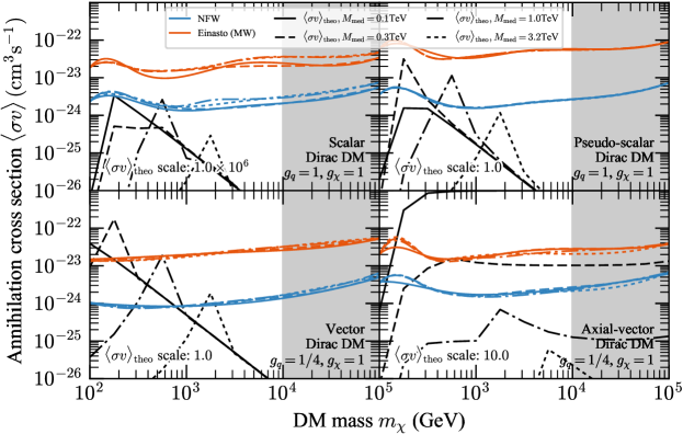
Figure 10: Examples for excluded annihilation cross sections for the different simplified models. Limits are shown for both considered DM density profiles (blue and orange lines) and for different mediator masses $M_{\mathrm{med}}=$ 0.1, 0.3, 1, and 3.2 TeV. Theoretical cross sections are also shown in black and are upscaled by a factor of $10^{6}$ and $10$ for the scalar and axial-vector DM, respectively. The NLO approximation of PPPC4DMID breaks down for $m_{\chi}>10\,$TeV, indicated by the gray shaded region.

For the points in the parameter space where $\langle\sigma v\rangle_{\mathrm{theo}}$ is larger than the limits on the cross section, these particular combinations of $M_{\mathrm{med}}$ and $m_{\chi}$ are ruled out (e.g. $m_{\chi}=0.2\,$TeV and $M_{\mathrm{med}}=0.3\,$TeV for the pseudoscalar case and the NFW DM density profile). These excluded regions of the parameter space are shown in Fig. 11 together with the combinations of $M_{\mathrm{med}}$ and $m_{\chi}$ that yield the correct relic abundance and limits from the LHC and DD. Only constraints for the pseudoscalar and vector DM models are presented. For scalar DM, none of the tested mass points are ruled out, due to the strong suppression of the theoretical annihilation cross section. In the EFT case this is reflected by the fact that none of the derived limits are in the EFT validity range. In the axial-vector case, CTA observations only rule out models for which the mediator masses are small but the DM mass is large. In this region, the model violates perturbative unitarity (see below).

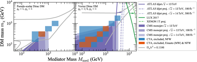
Figure 11: Projected limits and excluded values of $m_{\chi}$ vs $M_{\mathrm{med}}$ for the different DM models. CTA observations will exclude combinations of $m_{\chi}$ and $M_{\mathrm{med}}$ indicated by the orange (NFW and Einasto DM profiles) and blue (NFW only) squares. Only the parameter space to the right of the green and purple solid lines is allowed from current DD and dijet limits, respectively (dashed lines show projections of future searches). Purple regions show LHC monojet limits and projections. The gray lines show the parameter values that yield the correct relic abundance. No points are excluded in the scalar Dirac DM case for $g_{q}=g_{\chi}=1$ and none of the excluded parameters of the axial-vector model obey perturbative unitarity, thus these cases are not shown.

V.2.1 Relic Density

For simplified models, the nonrelativistic limit of the relic density calculation employed for the EFT scenario is no longer accurate. The addition of a mediator particle causes the nonrelativistic approximation of the annihilation rate to break down around the resonant enhancement region ($M_{\rm med}\simeq 2m_{\chi}$) and at the threshold of mediator production becoming kinematically accessible ($M_{\rm med}\lesssim m_{\chi}$).

The full relic density calculation entails solving the Boltzmann equation that determines the abundance of the DM particles at a given temperature, $Y(T)$, defined as the number density divided by the entropy density as follows, Gelmini et al. (1991); Edsjo and Gondolo (1997)

$$\frac{dY}{dT}=\sqrt{\frac{\pi g_{*}(T)}{45}}M_{\mathrm{Pl}}\langle\sigma v\rangle(Y(T)^{2}-Y_{\mathrm{eq}}(T)^{2})$$ (59)

where $g_{*}(T)$ is the temperature-dependent effective number of degrees of freedom, $Y_{\mathrm{eq}}(T)$ is the DM abundance in thermal equilibrium, and $\langle\sigma v\rangle$ is the relativistic thermally averaged DM annihilation cross section. The latter captures the specifics of each simplified model used here, including all possible annihilation channels. In the simplified models we study, we include only pair annihilations and no coannihilations, in which case the thermally averaged cross section is found to be Gondolo and Gelmini (1991)

$$\langle\sigma v\rangle=\frac{\int_{4m^{2}}^{\infty}dsK_{1}(\sqrt{s}/T)\sum\limits_{k,l}\sigma_{kl}(s-4m^{2})\sqrt{s}}{8m^{4}T\left(K_{2}(m/T)\right)^{2}}\;,$$ (60)

where $\sigma_{kl}$ is the total cross section for annihilation of a pair of particles with masses $m$ into the final states $(k,l)$, and $s$ is the invariant center-of-mass energy of the incoming particles. For instance, in the nonrelativistic limit, $\sqrt{s}$ is simply twice the DM mass. $K_{1}(K_{2})$ are the modified Bessel functions of order one (two). These modified Bessel functions arise as the result of the integrals involving the Boltzmann factors.

In order to compute the abundance of the DM particle today, $Y(T_{0})$, we integrate Eq. (59) from $T=\infty$ to $T=T_{0}$, leading to,

$$\Omega_{\chi}h^{2} = \frac{8\pi}{3}\frac{s(T_{0})}{M_{\mathrm{pl}}^{2}(100\,{\rm km\,s^{-1}\,Mpc^{-1}})^{2}}m_{\chi}Y(T_{0})$$ (61)

$$\approx 2.742\times 10^{8}\frac{m_{\chi}}{\mathrm{GeV}}Y(T_{0})$$

where $s(T_{0})$ is the entropy density today determined by the Planck Collaboration Ade et al. (2016). The procedure described above is handled numerically within micrOMEGAS Belanger et al. (2006). The resulting regions in the $M_{\mathrm{med}}$-$m_{\chi}$ parameter space that give the expected relic density are shown in Fig. 11 as gray lines.

The annihilation cross section into SM fermions given in Eq. (29) is proportional to $m_{q}^{2}/{m_{f}}^{2}$, whereas the annihilation into a pair of pseudoscalar fields does not depend on the quark masses. Therefore, in the former case annihilation into heavy quarks plays a crucial role, whereas in the latter the ratio $M_{\rm med}/m_{\chi}$ is the key quantity. With these features in mind one can understand the behavior of the curves for the relic density as shown in Fig. 11. One can see that when the DM mass becomes larger than the mediator mass, then the annihilation cross section in Eq. (35) simply depends on the ratio $M_{\rm med}/m_{\chi}$, explaining the behavior of the relic density curves. Using the same logic, when $m_{\chi}\gg M_{\rm med}$ the annihilation cross section in Eq. (35) becomes constant, explaining the horizontal lines for $M_{\rm med}<1$ TeV. The kinks exhibited by the relic density curves are a result of the top quark kinematic threshold. In other words, when annihilation into the top quarks is kinematically accessible, a sharp boost in the cross section takes place as a direct consequence of the $m_{q}^{2}/{m_{f}}^{2}$ enhancement.

In the vector mediator case, the DM annihilation cross section into SM fermions is very efficient, converse to the pseudoscalar case where there is a suppression proportional to the vacuum expectation value, since the vector mediator interaction with SM fermions is dictated by gauge symmetries. When the DM mass is much larger than the mediator mass, the annihilation cross section into fermions simply scales with $g_{q}^{2}g_{\chi}^{2}$, whereas the annihilation into the vector mediators goes with $g_{\chi}^{4}$. Hence, the annihilation cross section is constant since the couplings are fixed to be $g_{q}=0.25$, $g_{\chi}=1$, explaining the horizontal curves in Fig. 11. However, if $m_{\chi}\sim M_{\rm med}$, then annihilation into vector mediators becomes kinematically possible changing the overall shape of the annihilation cross section and relic density curves as can be seen in Fig. 11. A key feature of the vector mediator scenario is the pronounced resonance that happens for $M_{\rm med}\sim 2m_{\chi}$, which dominates the annihilation cross section then governed by the vector mediator decay width $\Gamma_{V,\rm tot}$.

We emphasize that we have assumed that DM annihilates into quarks only to facilitate comparisons with collider searches. However, the inclusion of other final states such as leptons and gauge bosons, would yield different predictions for the annihilation rates and introduce additional free parameters. This would also introduce a stronger dependence on a particular model. The inclusion of extra interactions is beyond the scope of this work which is focused on complementarity among different DM searches.

V.2.2 Direct detection

The DM-nucleon scattering in the nonrelativistic limit mediated by a pseudoscalar field leads to the spin-dependent momentum suppressed process. This momentum suppression arises when we match the quark-level matrix element with the nucleon-level matrix element in the nonrelativistic limit Freytsis and Ligeti (2011). Assuming $M_{\rm med}\gg t$ (where $t$ is the usual Mandelstam variable) the Lagrangian for the pseudoscalar mediator leads to the following scattering cross section,

$$\sigma^{SD}=\frac{9}{4}\frac{f_{N}^{2}}{m_{\chi}^{2}m_{N}^{2}}\frac{g_{\chi}^{2}\mu_{\chi N}^{2}}{M_{\rm med}^{4}}\,q^{4}$$ (62)

where $q$ is the momentum transfer, $N=n,p$, and,

$$f_{N} = m_{n}\left[\sum_{q=u,d,s}\frac{g_{q}}{{m_{f}}}\tilde{f_{q}}\right.$$ (63)

$$-\left.\bar{m}\left(\sum_{q=u,d,s}\frac{\tilde{f_{q}}}{m_{q}}\right)\sum_{q=u,d,s,c,t,b}\frac{g_{q}}{{m_{f}}}\right]$$

with $\bar{m}=(1/m_{u}+1/m_{d}+1/m_{s})^{-1}$ in agreement with Ref. Freytsis and Ligeti (2011), where $\tilde{f_{u}}=-0.44,\tilde{f_{d}}=0.84,\tilde{f_{s}}=-0.03$ Freytsis and Ligeti (2011); Cheng and Chiang (2012); Dienes et al. (2014). As in the EFT case, this expression can be directly compared to the limits reported by DD experiments. The momentum suppression in Eq. (62) causes the spin-dependent scattering cross section to lie orders of magnitude below current sensitivity. For couplings of order one and pseudoscalar masses above a few GeV, even the next generation of DD experiments will not furnish restrictive limits on the parameter space for the simplified model.

In contrast to the DM-nucleon scattering cross section, the annihilation cross section for pseudoscalar interaction between DM and quarks is not momentum suppressed due to the presence of an $s$-wave term in the cross section. This particular feature of the pseudoscalar interactions makes CTA well suited for these kinds of simplified DM models with the considered couplings, possibly outperforming collider and DD methods, depending on the true DM density profile in the GC. If the DM density follows the adopted NFW profile, it will also be possible to probe parameters that yield the correct DM relic density.

For the vector mediator case, things change dramatically, since the scattering is now spin independent and not velocity suppressed. The vector current is simply proportional to the number of valence quarks, and for this reason the calculation of WIMP-nucleon matrix element is not subject to large theoretical uncertainties Fitzpatrick et al. (2013). In the end the scattering cross section is found to be

$$\sigma^{SI}=\frac{9\mu_{\chi N}^{2}g_{\chi}^{2}g_{q}^{2}}{\pi M_{\rm med}^{4}}.$$ (64)

The limits from Ref. Akerib et al. (2017) and projections from Ref. Aprile et al. (2016b) are translated to limits in the $M_{\mathrm{med}}$-$m_{\chi}$ plane and shown as a green line in Fig. 11, excluding the region left of the line. Since we are adopting $g_{\chi}=1$ and $g_{q}=0.25$, the scattering cross section is large, and heavy mediators are needed to circumvent the DD limits.

V.2.3 LHC Constraints

LHC constraints on simplified DM models stem from searches for large missing energy events produced alongside with a visible counterpart such as a jet, lepton, or photon. For this reason such searches are generally referred to as mono-X searches. The properties of the model dictate which data set furnishes stronger limits. For the pseudoscalar mediator, monojet searches are the most restrictive. In Fig. 11 we show the monojet CMS constraints Sirunyan et al. (2017a). The LHC provides strong constraints at small masses but quickly loses sensitivity at higher energies (dark-purple shaded region in Fig. 11). We have used the Collider Reach tool col to estimate prospective reach at center-of-mass energy of 13  and 14 TeV and luminosities of 100 and 300 fb^-1, respectively (light-purple shaded regions in Fig. 11). CTA limits will be complementary to these constraints for mediator masses below 1 TeV, while becoming the discovery probe for higher DM and mediator masses.

As for the vector mediator cases, mono-X searches are no longer the most promising. In this case, searches for dijet resonances with large invariant mass are the most sensitive Alves et al. (2014); Abdallah et al. (2015); Chala et al. (2015); Sirunyan et al. (2016); Fairbairn et al. (2016). By imposing hard cuts in the invariant mass of the dijet events, one can reduce the large background from quantum chromodynamics and effectively search for (axial-)vector mediators. Such probes are particularly sensitive to the coupling $g_{q}$ and mediator mass. For this reason the dijet limit The ATLAS collaboration (2016) in Fig. 11 (blue solid line and blue dashed line for the sensitivity estimates) is fairly independent of the DM mass. Notice that in our simplified models, the mediators neither couple to leptons, the Higgs, nor to gauge bosons. We do not expect significant changes in the collider bounds with the inclusion of these interactions. For instance, with the inclusion of interactions with leptons, both vector and axial-vector mediator cases would be subject to a stronger collider limit by less than a factor of 2 on the $Z^{\prime}$ mass Alves et al. (2015). This more restrictive bound would stem from resonance searches for dilepton final states at the LHC, which typically give rise to tighter constraints than the dijet one Alves et al. (2015).

V.2.4 Unitarity/perturbativity

The simplified model paradigm assumes that some unspecified UV completion assures the consistency of the model, providing a mechanism for mass generation and ensuring features such as gauge invariance. However, the axial-vector model includes processes which can violate gauge invariance and perturbative unitarity in certain regions of parameter space, such that any UV completion would fundamentally alter the phenomenology of the model in these regions Kahlhoefer et al. (2016). In order to ensure that the model does not violate perturbative unitarity, the following conditions must be met:

$$m_{\chi,q} \lesssim \sqrt{\frac{\pi}{2}}\frac{M_{\rm med}}{g_{\chi,q}},$$ (65)

$$\sqrt{s} < \frac{\pi M_{\rm med}^{2}}{g_{\chi}^{2}m_{\chi}}.$$ (66)

For ID, $\sqrt{s}\simeq 2m_{\chi}$, and Eq. (66) reduces to Eq. (65). For the chosen values of $g_{\chi}$ and $g_{q}$, the criteria are not met by the combinations of $m_{\chi}$ and $M_{\mathrm{med}}$ that CTA observations could test.

VI Conclusions

In this article, we have compared the sensitivity of the future CTA to constrain annihilating DM with exclusions obtained from DD experiments and DM searches at the LHC. This comparison has been achieved by utilizing the frameworks of EFTs and simplified models. Our sensitivity projections are based on realistic IACT observation schemes of the Galactic center and test two different DM density profiles which are compatible with recent observations. They also incorporate contributions from Galactic diffuse emission and possible systematic uncertainties.

Within EFTs and simplified models, it is straightforward to compare the derived sensitivity with limits and projections from DD experiments and collider searches for DM at the LHC. This is not the case for limits that are reported for a pure annihilation into one particular channel. We have found that for DM mediators for which the annihilation is neither velocity nor helicity suppressed (pseudoscalar and vector mediators; cf. Table 1), CTA will be able to probe regions of the parameter space out of reach for present and possibly even future collider searches (Figs. 9 and 11). It will also be possible to probe parts of the parameter space that results in the correct DM relic abundance. In the case of vector mediated DM, strong constraints already exist from DD experiments and LHC dijet analyses, and CTA observations are unlikely to improve on already existing bounds, but it will still introduce a compelling and orthogonal probe to the model. The situation is however different if the DM mediator is a pseudoscalar. In this case, the scattering cross section is suppressed by a combination of the DM spin and spin of the nucleus. Indeed, the scattering cross section is spin dependent and momentum suppressed at the fourth power rendering DD bounds to be very suppressed. Each $\gamma_{5}$ matrix in the Lagrangian for the pseudo scalar model results in a momentum suppression, yielding a suppression proportional to $q^{4}$, where $q$ is the momentum transfer, in the WIMP-nucleon scattering. Moreover, because in this model the couplings with quarks have a Yukawa-like structure, suppressed by the fermion mass, dijet limits are not very competitive, and thus far there is no dijet limit from LHC for this simplified model.

For such DM models, CTA observations will be indispensable to probe higher values of DM (and mediator masses). In the EFT framework, the derived limits only depend weakly on the assumed DM density profile in the Milky Way due to strong dependence of the EFT scale $M_{\star}$ on the limits on the annihilation cross section. This is not the case for simplified models where the limits strongly degrade from the considered NFW to the Einasto density profile (cf. Fig. 11). To summarize, our results illustrate the need for different techniques (DD, ID, collider searches) to probe all possibilities of DM models.

We stress that all calculations presented here assume 100 hours of observation time of the Galactic center (and additionally 200 hours in the case of an Einasto density profile for independent background determination). Such an observational program should be completed within the first years of CTA operation. Therefore, the projected limits are bound to improve as CTA will continue to observe the GC beyond the first years of operation (the limits are expected to improve roughly with the square root of observation time). Furthermore, several analysis choices should be optimized in future analyses, such as the choice of the spectral and spatial binning, as well as the treatment of systematic uncertainties and GDE. For the GDE, a simple power-law extrapolation of the template provided by the Fermi-LAT Collaboration was used here that likely overestimates the GDE contribution at very high energies. A careful treatment of the GDE and optimization of the analysis parameters will be conducted in a forthcoming publication of the CTA consortium.