Quantum lattice Boltzmann study of random-mass Dirac fermions in one dimension

Abstract

We study the time evolution of quenched random-mass Dirac fermions in one dimension by quantum lattice Boltzmann simulations. For nonzero noise strength, the diffusion of an initial wave packet stops after a finite time interval, reminiscent of Anderson localization. However, instead of exponential localization we find algebraically decaying tails in the disorder-averaged density distribution. These qualitatively match $\propto x^{-3/2}$ decay, which has been predicted by analytic calculations based on zero-energy solutions of the Dirac equation.

I Introduction

It is a great pleasure, let alone honor, to present this contribution on the occasion of Prof. Norman H. March 90th Festschrift. Prof. March made many distinguished contributions across a broad variety of topics in classical and quantum statistical physics; in the following we present a computational investigation along the latter direction, namely the transport properties of random-mass Dirac fermions in $1+1$ dimensions.

Disorder plays an important role in many physical systems, ranging from topological materials Groth et al. (2009); Kobayashi et al. (2014); Morimoto et al. (2015); Bagrets et al. (2016) to transport properties affected by impurities, superconductors Seo et al. (2014) and glasses Yunker et al. (2010). In condensed matter physics, a prominent effect of disorder is exponential Anderson localization of the electronic wavefunction Anderson (1958), which has been experimentally observed in Bose-Einstein condensates Billy et al. (2008). Nevertheless, around critical points there can be transitions away from the localized phase Balents and Fisher (1997); Shelton and Tsvelik (1998); Mkhitaryan and Raikh (2011). In one dimension, similarities between these delocalized phases and classical particle motion in a stationary random potential with a variety of diffusion laws Sinai (1982); Bouchaud et al. (1990); Comtet and Dean (1998) have been pointed out, including anomalously slow Sinai diffusion $|x|\propto\log(t)^{2}$ Bagrets et al. (2016).

In this work, we study the time evolution dynamics governed by a prototypical random-mass Dirac equation in one dimension, and investigate the fate of an initial Gaussian wave packet. The general framework is similar to a recent related work Yosprakob and Suwanna (2016), except for the numerical quantum lattice Boltzmann approach pursued here, and different versions of the Dirac equation. Specifically, using the Majorana representation and projecting upon chiral eigenstates (and setting $\hbar=1$), the Dirac equation considered here reads

$$\big{(}i\partial_{t}+ic\sigma^{z}\partial_{x}+c^{2}m(x)\sigma^{y}\big{)}\psi(x,t)=0,$$ (1)

where $\psi(x,t)$ is a two-component spinor, $\sigma^{\alpha}$ are the Pauli matrices, $c$ the speed of light, and $m(x)$ is the spatially dependent mass. We model quenched disorder by taking $m(x)$ as a Gaussian white noise random variable with mean $m_{0}$ and noise strength $\lambda$:

$$\langle(m(x)-m_{0})(m(x^{\prime})-m_{0})\rangle=2\lambda\delta(x-x^{\prime}).$$ (2)

The spinor $\psi=(u,d)^{T}$ consists of the chiral right-moving ($u$) and left-moving ($d$) states. The stationary version of Eq. (1) (without the time derivative) has been identified as an effective theory in a tight-binding model of spinless fermions Balents and Fisher (1997).

The dynamics governed by (1) conserves total density and energy. For example, the local density

$$\rho=|\psi|^{2}=|u|^{2}+|d|^{2}$$ (3)

obeys the conservation law

$$\partial_{t}\rho(x,t)+\partial_{x}J_{\rho}(x,t)=0$$ (4)

with the density current

$$J_{\rho}(x,t)=c\left(|u|^{2}-|d|^{2}\right).$$ (5)

We will see in the numerical simulations that $\psi(x,t)$ converges to a stationary state for $\lambda>0$; this stationary state can thus be compared to the zero-energy solution studied in Balents and Fisher (1997): $\psi(x)=\psi_{\pm}(x)(\begin{smallmatrix}1\\ \mp 1\end{smallmatrix})$, with the scalar function $\psi_{\pm}(x)$ satisfying

$$\big{(}\partial_{x}\pm cm(x)\big{)}\psi_{\pm}(x)=0.$$ (6)

For “critical” zero average mass ($m_{0}=0$), this results in the log-normally distributed wavefunction

$$\psi_{\pm}(x)\propto\mathrm{e}^{\pm\int_{0}^{x}cm(x^{\prime})\mathrm{d}x^{\prime}},$$ (7)

which deviates from exponential localization. By a mapping to Liouville field theory, the disorder-averaged spatial correlations of the wavefunction (7) can be computed analytically Balents and Fisher (1997); Shelton and Tsvelik (1998); Steiner et al. (1998), resulting in an algebraic (instead of exponential) decay with exponent $-3/2$:

$$\left\langle\lvert\psi(x)\rvert^{2}\lvert\psi(0)\rvert^{2}\right\rangle\propto\lvert x\rvert^{-3/2}.$$ (8)

Thus, disorder in the random mass distribution does not lead to Anderson localization if the average mass is zero.

II Quantum lattice Boltzmann method

Eq. (1) lends itself to a lattice Boltzmann discretization for the spinor components $u$ and $d$, as observed in Succi and Benzi (1993); Palpacelli and Succi (2008); Fillion-Gourdeau et al. (2013). The propagation step consists of streaming $u$ and $d$ along the $x$-axis with opposite speeds $\pm c$, while the collision step is performed according to the scattering term $c^{2}m(x)\sigma^{y}\psi$. Integrating (1) along the characteristics of $u$ and $d$, respectively, and approximating the collision integral by the trapezoidal rule, the following relations are obtained:

$$\begin{split}\hat{u}-u&=\tilde{m}(d+\hat{d})/2\\ \hat{d}-d&=-\tilde{m}(u+\hat{u})/2,\end{split}$$ (9)

where $\hat{u}=u(x+\Delta x,t+\Delta t)$, $\hat{d}=d(x-\Delta x,t+\Delta t)$, $\Delta x=c\Delta t$, and $\tilde{m}=c^{2}m\Delta t$. Algebraically solving the linear system (9) yields the explicit scheme

$$\begin{pmatrix}\hat{u}\\ \hat{d}\end{pmatrix}=\begin{pmatrix}a&b\\ -b&a\end{pmatrix}\begin{pmatrix}u\\ d\end{pmatrix},$$ (10)

with

$$a=(1-\tilde{m}^{2}/4)/(1+\tilde{m}^{2}/4),\quad b=\tilde{m}/(1+\tilde{m}^{2}/4).$$

Note that, since $|a|^{2}+|b|^{2}=1$, the collision matrix is unitary, thus the method is unconditionally stable and norm-preserving.

III Numerical simulation results

We start from a “wave packet” initial state given by

$$\psi(x,0)\equiv\begin{pmatrix}u\\ d\end{pmatrix}=\big{(}\sqrt{8\pi}\sigma\big{)}^{-1/2}\mathrm{e}^{-x^{2}/4\sigma^{2}}\begin{pmatrix}1\\ 1\end{pmatrix},$$ (11)

with the standard deviation $\sigma$ measuring the width of the wave packet, and the normalization chosen such that $\int_{-\infty}^{\infty}\rho(x,t)\,\mathrm{d}x=1$ at $t=0$. Due to density conservation, this relation holds for all $t$.

Table 1 lists the simulation parameters in detail. The speed of light $c=\Delta x/\Delta t=1$, and the physical simulation domain is the interval $[-64,64]$.

$L$	2048	system size (number of grid points) with periodic boundary conditions
$\Delta x$	$1/16$	grid spacing
$\Delta t$	$1/16$	time step
$\sigma$	$1$	standard deviation of initial spinor
$n_{\text{runs}}$	$10^{5}$	number of random mass realizations (simulation runs) to compute averages $\langle\dots\rangle$
$n_{\text{cut}}$	$256$	cut-off Fourier mode of random mass distribution

Table 1: Simulation parameters

Eq. (2) suggests to draw a random $m(x_{i})$ independently at each grid point $x_{i}$. However, this would render the simulation sensitive to the grid spacing $\Delta x$. Instead, we draw independent Fourier coefficients up to some cut-off Fourier mode $n_{\text{cut}}$, and then transform to real space to obtain a random mass realization. Thus, the grid resolution is much finer than random mass oscillations. The random mass correlations obtained by this procedure decay on a length scale $x-x^{\prime}=\Delta xL/(2n_{\text{cut}})$. This quantity is chosen small compared to the width of the initial wave packet, in order to approximate the delta function in Eq. (2).

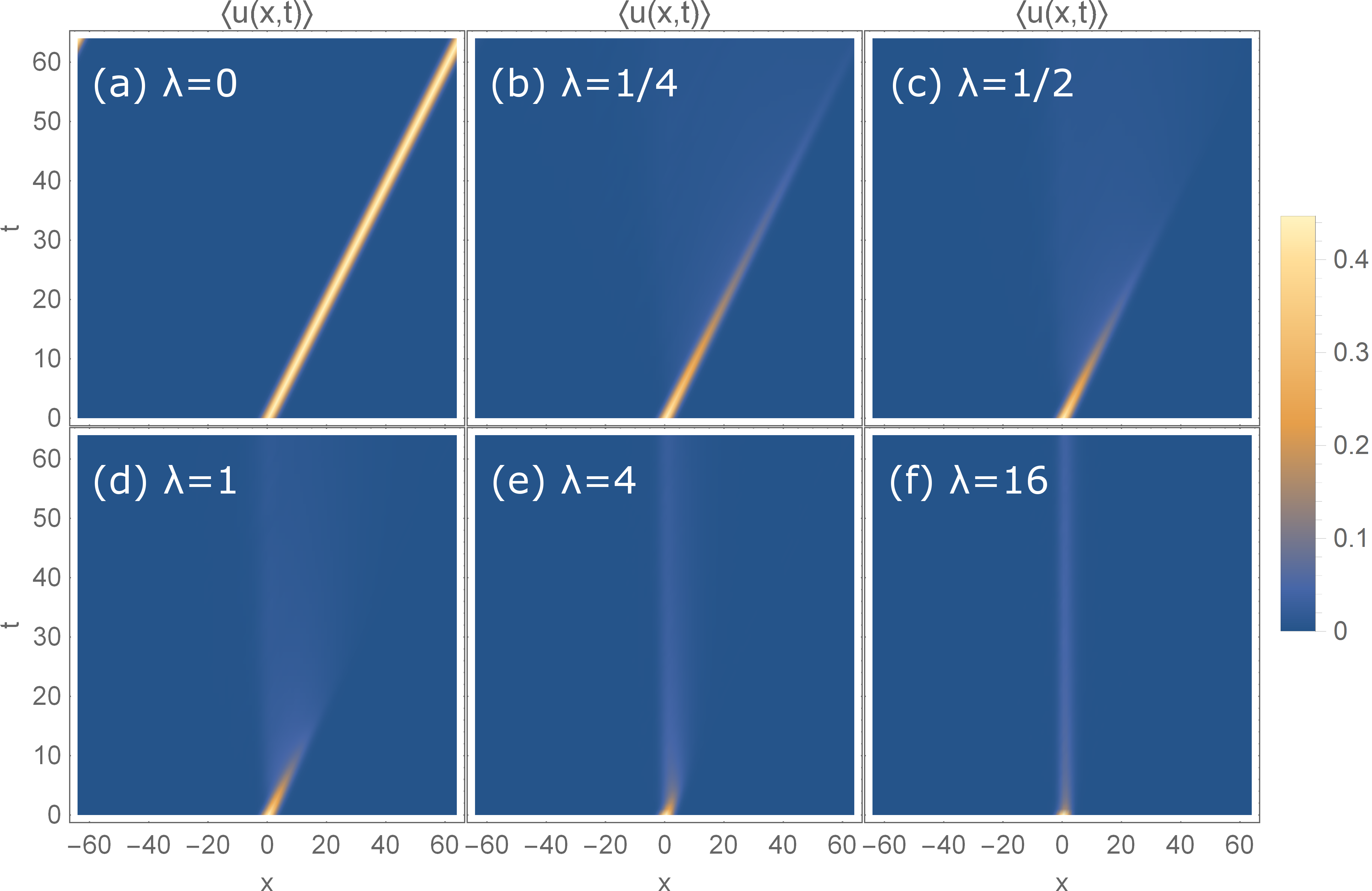
Figure 1: Average $\langle u(x,t)\rangle$ profile for increasing noise strength of the random mass distribution, and $m_{0}=0$.

Fig. 1 shows $\langle u(x,t)\rangle$ for various values of $\lambda$, for zero average mass ($m_{0}=0$). In the absence of noise ($\lambda=0$), there is no scattering term in the Dirac equation, and the $u$ and $d$ waves freely propagate to the right and left, respectively. For $\lambda>0$, the right-moving ray is continuously diminished over time due to scattering. As $\lambda$ increases, the wave packet remains more and more tied to the origin.

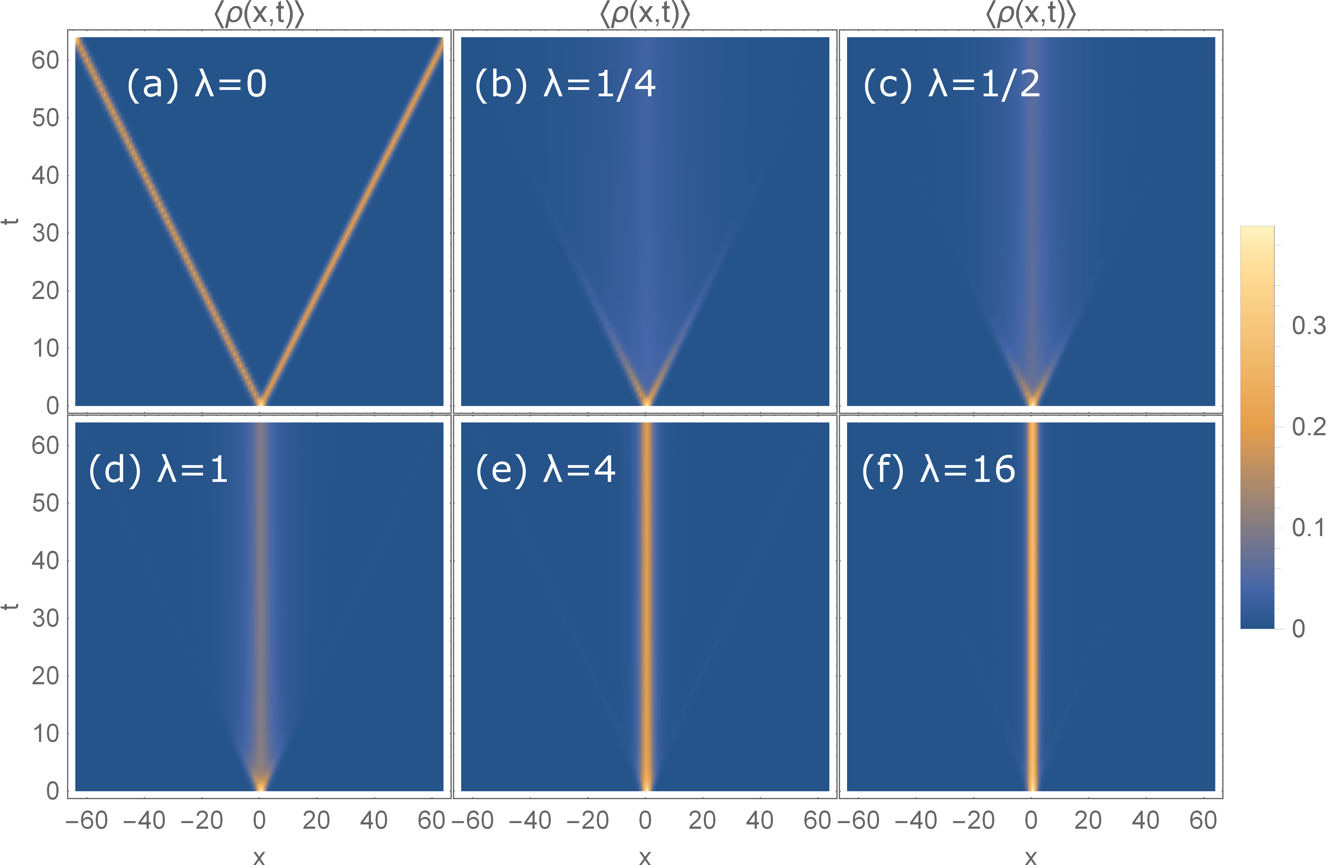
Figure 2: Average density $\langle\rho(x,t)\rangle$ for increasing noise strength of the random mass distribution, and $m_{0}=0$.

Fig. 2 visualizes the corresponding density profiles $\langle\rho(z,t)\rangle$ for the same simulations. For any $\lambda>0$, one observes remnant density centered around the origin. The density profile remains stationary at later times.

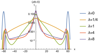
Figure 3: Average density $\langle\rho(x,t)\rangle$ at $t=60$ on a logarithmic scale, for $m_{0}=0$.

To analyze the noise-averaged density quantitatively, Fig. 3 shows the density profile on a logarithmic scale at $t=60$, when it has (almost) reached stationarity between the left- and right-moving sound peaks around $x\simeq\pm 60$. The density decays exponentially with respect to $|x|$ for $0<\lambda\lesssim 1$, different from the predicted algebraic decay in Eq. (8). One explanation could be that the algebraic decay sets in at larger $|x|$. On the other hand, for $\lambda\gtrsim 4$, one observes a transition from exponential to slower-decaying tails. (Note that for the particular initial condition used in our simulations, we find that the density correlation between the the origin and $x$ is proportional to the density profile.)

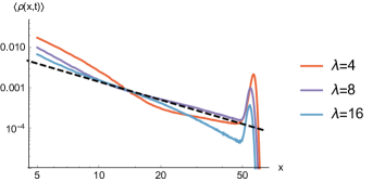
Figure 4: Average density $\langle\rho(x,t)\rangle$ at $t=60$ on a log-log scale, for $m_{0}=0$. For comparison, the black dashed line is $\propto x^{-3/2}$.

Fig. 4 shows these tails on a log-log scale, which indeed ascertains an algebraic decay at larger $\lvert x\rvert$. Between $20<x<45$, the curve for noise strength $\lambda=4$ decays somewhat slower, the $\lambda=16$ curve somewhat faster, and the $\lambda=8$ curve almost exactly as the black dashed $\propto x^{-3/2}$ line based on the theoretical prediction (8).

The logarithmic scale in Fig. 3 shows that the outward-moving sound peaks are present also for $\lambda\geq 1$, even though not visible in Fig. 2. The effective sound velocity $v_{\text{eff}}$ (measured via the peak maximum) monotonically decreases with noise strength, as expected (see Fig. 5).

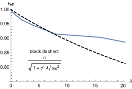
Figure 5: Measured sound velocity in dependence of noise strength $\lambda$, for $m_{0}=0$.

Solutions of the free Dirac equation also solve the Klein-Gordon equation with dispersion relation $\omega^{2}=(ck)^{2}+\omega_{c}^{2}$, where $\omega_{c}=c^{2}m/\hbar$ is the Compton frequency. The corresponding sound speed is therefore

$$v_{\text{KG}}=\partial_{k}\omega=\frac{c}{\sqrt{1+(\omega_{c}/(ck))^{2}}}.$$ (12)

The wave number $k$ should be inversely proportional to the spatial extent of the wave packet; thus we approximate $ck\simeq\omega_{0}$ with $\omega_{0}=2\pi c/\sigma$. For the Compton frequency, we use $\sqrt{\lambda}$ as proxy for the mass term, and set $\hbar=1$ as before. This results in the black dashed curve in Fig. 5, which indeed qualitatively reproduces the measured sound velocity up to $\lambda\lesssim 8$.

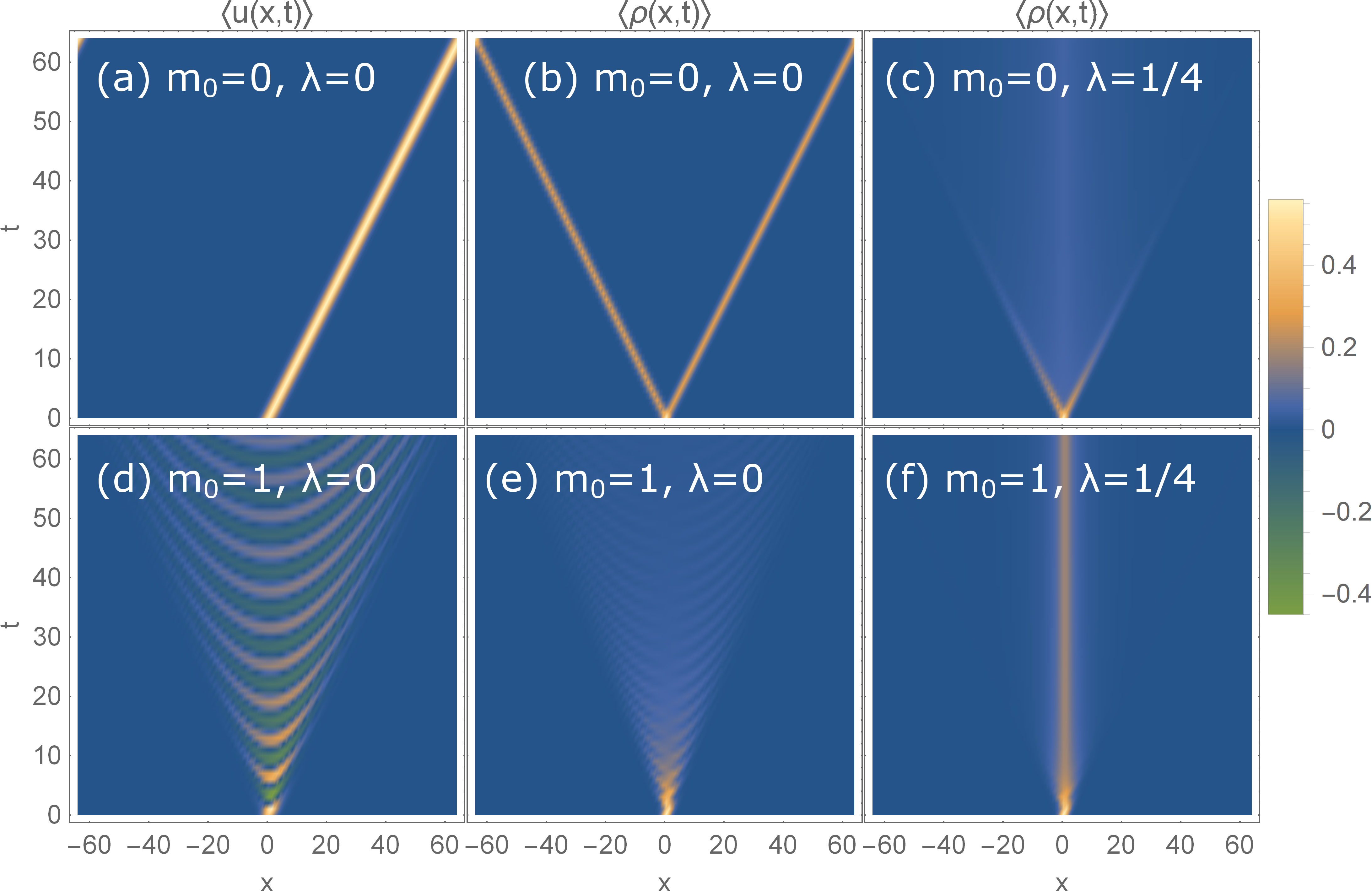
Figure 6: Comparison of the $\langle u(x,t)\rangle$ profile and density $\langle\rho(x,t)\rangle$ for $m_{0}=0$ (top row) with $m_{0}=1$ (bottom row).

Tuning away from zero average mass should result in “conventional” exponentially localized wavefunctions (see also Eq. (7)) at zero-energy. Fig. 6 directly compares hitherto $m_{0}=0$ simulations with $m_{0}=1$. Without disorder ($\lambda=0$), the $u$ (and $d$) component exhibits a parabola-shaped stripe pattern (see Fig. 6d), instead of linear propagation. The corresponding density has a more uniform profile. When including disorder ($\lambda=1/4$), one notices that the average density is more strongly confined for $m_{0}=1$ (Fig. 6f) than for $m_{0}=0$ (Fig. 6c).

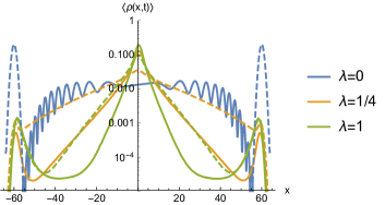
Figure 7: Average density $\langle\rho(x,t)\rangle$ for $m_{0}=1$ (solid lines) compared to $m_{0}=0$ (dashed lines, same data as in Fig. 3).

This stronger confinement is confirmed in Fig. 7, which compares the densities on a logarithmic scale for $0\leq\lambda\leq 1$. Besides the oscillatory pattern at $\lambda=0$, the density for $m_{0}=1$ decays faster than for $m_{0}=0$ at fixed $\lambda>0$.

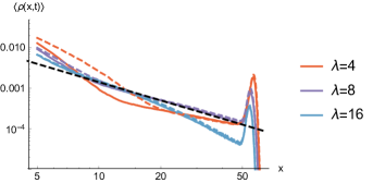
Figure 8: Average density $\langle\rho(x,t)\rangle$ on a log-log scale for $m_{0}=1$ (solid lines) compared to $m_{0}=0$ (dashed lines, same data as in Fig. 4).

Fig. 8 compares the densities on a log-log scale for $\lambda\geq 4$. Somewhat surprisingly, the non-zero average mass $m_{0}=1$ does not affect the algebraic decay, although one would expect exponential decay away from the “critical” $m_{0}=0$. An explanation could be that large values of the noise override small changes in the average mass.

IV Conclusions and outlook

We have shown that quantum lattice Boltzmann methods can efficiently simulate the real-time dynamics of the single-particle Dirac equation (1) for random-mass fermions in one spatial dimension. Since the quantum lattice Boltzmann scheme is not limited to one-dimensional systems Dellar et al. (2011), for the future it would be interesting to study the transport properties of random-mass fermions in two and three spatial dimensions. Besides analyzing stationary properties, lattice Boltzmann simulations of the Dirac equation could also be used for investigating the time dynamics of out-of-equilibrium systems, including, e.g., thermalization and quasiparticle lifetime, cf. Succi (2015). Work along the lines is currently underway.