Quantum correlations and degeneracy of identical bosons in a 2D harmonic trap

Abstract

We consider a few number of identical bosons trapped in a 2D isotropic harmonic potential and also the $N$-boson system when it is feasible. The atom-atom interaction is modelled by means of a finite-range Gaussian interaction. The spectral properties of the system are scrutinized, in particular, we derive analytic expressions for the degeneracies and their breaking for the lower-energy states at small but finite interactions. We demonstrate that the degeneracy of the low-energy states is independent of the number of particles in the noninteracting limit and also for sufficiently weak interactions. In the strongly interacting regime, we show how the many-body wave function develops holes whenever two particles are at the same position in space to avoid the interaction, a mechanism reminiscent of the Tonks-Girardeau gas in 1D. The evolution of the system as the interaction is increased is studied by means of the density profiles, pair correlations and fragmentation of the ground state for $N=2$, $3$, and $4$ bosons.

I Introduction

The problem of a particle trapped in a harmonic trap is one of the best known quantum systems. Going from a single particle to a system composed of $N$ interacting particles is, however, far more involved. Interestingly, recent advances in ultracold atomic gases have opened the possibility of studying systems of a few atoms, either fermions or bosons, trapped in potentials of different kind Zurn ; Bakr ; Sherson ; Islam .

For the bosonic case, there are important results in 1D where the fermionization of the bosonic gas was preconized by Tonks and Girardeau Girardeau for the case of infinitely repulsive bosons and later confirmed experimentally in ultracold atomic gases Paredes ; Kinoshita . There are many works studying fermionization in 1D, for instance, in optical lattices Pupillo , in few-atom mixtures Garcia-March4 ; Garcia-March ; Pyzh , for attractive interactions Tempfli and for few dipolar bosons Deuretzbacher . In other cases, the focus are quantum correlations Koscik ; Barfknecht , its effects in mixtures of distinguishable and identical particles Garcia-March3 and analytic ansatz to capture the physics in all interaction regimes Wilson .

The case of two particles with contact interactions was considered in one, two and three dimensions in Ref. Busch . There, they obtained semi-analytic results finding the energies and wave functions as solution of transcendental equations. More general cases of few-body systems have been studied mostly in 3D, see Ref. Blume_Report and references therein.

In 2D, semi-analytical approximate solutions to the case of two bosons with finite range interactions have been presented in Ref. Doganov . Other 2D works include two and three-body exact solutions for fermions and bosons with contact interaction Liu , fast-converging numerical methods for computing the energy spectrum for a few bosons Christensson , the study of finite-range effects Imran ; Imran2 and universality Kartavtsev ; Shea , condensation in trapped few-boson systems Daily , and interacting few-fermions systems Stetcu ; Liu2 .

In this paper, we study the properties for $N=2$, $3$, and $4$ identical bosons interacting through a finite-range interaction confined in a 2D isotropic harmonic trap by means of direct diagonalization of the Hamiltonian.

We analyze the properties of the system as we increase the strength of the interaction, going from the noninteracting regime to the strongly interacting one. In Sect. II, we present the many-body Hamiltonian, including the two-body Gaussian-shaped interaction potential considered. We split the center-of-mass and relative parts of the Hamiltonian making use of Jacobi coordinates. In Sect. III, we consider first the noninteracting Hamiltonian and discuss in some details the degeneracies present in the many-body spectrum. In Sect. IV, we focus on the effect of interactions on the many-body spectrum of the system. In Sect. V, we discuss the correlations which build in the ground state as the interaction is increased. Finally, the conclusions and summary are presented in Sect. VI.

II The $N$-boson Hamiltonian

We consider a system of $N$ identical bosons of mass $m$ trapped by an isotropic harmonic potential. The many-body Hamiltonian in first quantized form reads

$${\cal H}=\sum_{i=1}^{N}\left(-\frac{\hbar^{2}}{2m}\nabla^{2}_{i}+\frac{1}{2}m\omega^{2}\vec{x}^{\,2}_{i}\right)+g\,\sum_{i<j}^{N}V(\vec{x}_{i}-\vec{x}_{j})\,.$$ (1)

In usual ultracold atomic gases experiments, the atom-atom interactions are well approximated by a contact potential. In our case, we use a finite-size Gaussian potential,

$$V(\vec{x}_{i}-\vec{x}_{j})=g\;\frac{1}{\pi s^{2}}e^{-\frac{(\vec{x}_{i}-\vec{x}_{j})^{2}}{s^{2}}}\,,$$ (2)

where $g$ and $s$ characterize the strength and range of the interaction, respectively. Both parameters are considered to be tuneable. For instance, $g$ can be varied by means of a suitable Feshbach resonance. In the limit of $s$ going to zero, we recover a contact interaction with strength $g$. Regardless of $N$, we can split the Hamiltonian in two parts, ${\cal H}={\cal H}_{\rm cm}+{\cal H}_{\rm r}$, using Jacobi coordinates,

$$\vec{R} \equiv \frac{1}{N}\sum_{i=1}^{N}\vec{x}_{i}\,,$$ (3)

$$\vec{r}_{k} \equiv \sqrt{\frac{2k}{k+1}}\left(\vec{x}_{k+1}-\frac{1}{k}\sum_{i=1}^{k}\vec{x}_{i}\right),\,\,k=1,\,...\,,N-1\,.$$

The center-of-mass part and relative part of the total Hamiltonian read

$${\cal H}_{\rm cm}=-\frac{\hbar^{2}}{2M}\nabla^{2}_{\vec{R}}+\frac{1}{2}M\omega^{2}\vec{R}^{\,2},$$ (4)

$${\cal H}_{\rm r}=\sum_{k=1}^{N-1}\left(-\frac{\hbar^{2}}{2\mu}\nabla^{2}_{\vec{r}_{k}}+\frac{1}{2}\mu\omega^{2}\vec{r}^{\,2}_{k}\right)+g\tilde{V}(\vec{r}_{1},...\,,\vec{r}_{N-1}),$$ (5)

with the definitions $M\equiv Nm$ and $\mu\equiv m/2$. The interaction only appears in the relative part and takes the form

$$\begin{gathered}\tilde{V}(\vec{r}_{1},...\,,\vec{r}_{N-1})\equiv\\ \sum_{i<j}^{N}V\left(\vec{x}_{i}(\vec{R},\vec{r}_{k},...\,,\vec{r}_{N-1})-\vec{x}_{j}(\vec{R},\vec{r}_{k},...\,,\vec{r}_{N-1})\right)\,.\end{gathered}$$ (6)

As a consequence, the change in the energy spectrum with increasing the interaction through $g$ or changing the range $s$ will come from a change in the energy associated to ${\cal H}_{\rm r}$.

II.1 Second-quantized $N$-boson Hamiltonian

Our numerical method to study the excitation spectrum will consist in truncating the Hilbert space of the $N$-boson system such that the particles can populate only the first $M$ single-particle eigenstates. We label the single particle states, $\psi_{i}(x,y)$, and their corresponding eigenenergies, $\epsilon_{i}=n_{x}+n_{y}+1$, with an index $i=1,\,...\,,M$ running through the pair of quantum numbers $n_{x}$ and $n_{y}$. With this truncation, the second quantized Hamiltonian reads

$$\hat{H}=\hat{H}_{0}+\hat{H}_{\rm int}\,.$$ (7)

Where $\hat{H}_{0}$ and $\hat{H}_{\rm int}$ correspond to the single particle and interaction terms,

$$\hat{H}_{0} = \sum_{i=1}^{M}\hat{a}^{\dagger}_{i}\hat{a}_{i}\,\epsilon_{i}\,,$$

$$\hat{H}_{\rm int} = \frac{g}{2}\sum_{i,j,k,l=1}^{M}\hat{a}^{\dagger}_{i}\hat{a}^{\dagger}_{j}\hat{a}_{k}\hat{a}_{l}\,V_{i,j,k,l}\,,$$ (8)

where

$$V_{i,j,k,l} = \frac{1}{\pi s^{2}}\int_{-\infty}^{\infty}dx\,dy\,dx^{\prime}\,dy^{\prime}\,\psi^{*}_{i}(x,y)\psi_{k}(x,y)$$ (9)

$$\times \psi^{*}_{j}(x^{\prime},y^{\prime})\psi_{l}(x^{\prime},y^{\prime})\;e^{-\frac{(x-x^{\prime})^{2}+(y-y^{\prime})^{2}}{s^{2}}}.$$

The explicit analytical form of these integrals, $V_{i,j,k,l}$, is provided in Appendix C.

The operator $\hat{a}^{\dagger}_{i}$($\hat{a}_{i}$) creates(destroys) a particle in the single particle mode $i$,

$$\hat{a}^{\dagger}_{i}\ket{n_{1},\,...\,,n_{M}} = \sqrt{n_{i}+1}\ket{n_{1},\,...\,,n_{i}+1,\,...\,,n_{M}}\,,$$

$$\hat{a}_{i}\ket{n_{1},\,...\,,n_{M}} = \sqrt{n_{i}}\ket{n_{1},\,...\,,n_{i}-1,\,...\,,n_{M}}\,.$$ (10)

They satisfy bosonic commutation relations, $[{\hat{a}}_{i},{\hat{a}}^{\dagger}_{j}]=\delta_{i,j}$. We introduce the Fock basis,

$$\ket{n_{1},\,...\,,n_{M}}=\frac{(\hat{a}^{\dagger}_{1})^{n_{1}}\dots(\hat{a}^{\dagger}_{M})^{n_{M}}}{\sqrt{n_{1}!\,...\,n_{M}!}}\ket{\rm vac},$$ (11)

where $\ket{\rm vac}\equiv\ket{0,\,...\,,0}$ is the vacuum state and, as we consider a fixed number of particles $N$, the quantum numbers $n_{i}$ verify

$$N=\sum_{i=1}^{M}n_{i}\,.$$ (12)

The dimension of the Fock space is

$$D_{N}^{M}=\frac{(M+N-1)!}{(M-1)!N!},$$ (13)

which, for $N=2$, $3$, and $4$, gives, respectively,

$$D_{2}^{M} = \frac{M(M+1)}{2}\,,$$

$$D_{3}^{M} = \frac{M(M+1)(M+2)}{6}\,,$$

$$D_{4}^{M} = \frac{M(M+1)(M+2)(M+3)}{24}\,.$$ (14)

III Degeneracies in the noninteracting limit

In this section, we will discuss the degeneracies present in the system in absence of interactions. First, we consider the two-boson case, in which the analysis is simpler, and then we shall explain the main degeneracies for $N$ bosons.

III.1 The two-boson system

In the noninteracting case, $g=0$, for the two-boson system, we can write down the Hamiltonian in second quantization, splitting the center of mass and the relative motion. Using from now on harmonic oscillator units, $\hbar\omega$ for energy and $\sqrt{\hbar/(m\omega)}$ for length, we have, in polar coordinates,

$$\hat{H}=\hat{H}_{\rm cm}+\hat{H}_{\rm r}=\hat{n}_{\rm cm}+\hat{n}_{r}+2,$$ (15)

where $\hat{H}_{\rm cm}=\hat{n}_{\rm cm}+1$, $\hat{H}_{r}=\hat{n}_{r}+1$. Therefore, we have a 2D harmonic oscillator for each part of the Hamiltonian. The corresponding eigenstates can be labelled as $\ket{n_{\rm cm},m_{\rm cm},n_{r},m_{r}}$, namely,

$$\hat{n}_{\rm cm}\ket{n_{\rm cm},m_{\rm cm},n_{r},m_{r}} = n_{\rm cm}\ket{n_{\rm cm},m_{\rm cm},n_{r},m_{r}},$$

$$\hat{n}_{r}\ket{n_{\rm cm},m_{\rm cm},n_{r},m_{r}} = n_{r}\ket{n_{\rm cm},m_{\rm cm},n_{r},m_{r}},$$

$$\hat{L}_{z,\rm cm}\ket{n_{\rm cm},m_{\rm cm},n_{r},m_{r}} = m_{\rm cm}\ket{n_{\rm cm},m_{\rm cm},n_{r},m_{r}},$$

$$\hat{L}_{z,r}\ket{n_{\rm cm},m_{\rm cm},n_{r},m_{r}} = m_{r}\ket{n_{\rm cm},m_{\rm cm},n_{r},m_{r}},$$

where $\hat{L}_{z,\rm cm}$ and $\hat{L}_{z,\rm r}$ are the third component of the center-of-mass orbital angular momentum and the relative orbital angular momentum, respectively, expressed in units of $\hbar$. However, those four quantum numbers have a restriction imposed by the symmetry of the wave function under the exchange of particles. The full wave function in polar coordinates for $\vec{R}$ and $\vec{r}$ reads

$$\begin{gathered}\chi_{n_{\rm cm},m_{\rm cm},n_{r},m_{r}}\left(R,r,\varphi_{R},\varphi_{r}\right)=\\ \chi_{n_{\rm cm},m_{\rm cm}}\left(\sqrt{2},R,\varphi_{R}\right)\chi_{n_{r},m_{r}}\left(\frac{1}{\sqrt{2}},r,\varphi_{r}\right),\end{gathered}$$

with

$$\begin{split}\chi_{n,m}\left(\alpha,r,\varphi\right)=N_{n,m}\left(\alpha\right)e^{im\varphi}\\ \times\,e^{-\frac{\left(\alpha r\right)^{2}}{2}}\left(\alpha r\right)^{|m|}L^{|m|}_{\frac{n-|m|}{2}}\left(\left(\alpha r\right)^{2}\right)\,.\end{split}$$ (17)

The $L^{k}_{n}(x)$ are the associated Laguerre polynomials defined as

$$L^{k}_{n}(x)\equiv\sum_{m=0}^{n}(-1)^{m}\begin{pmatrix}n+k\\ n-m\end{pmatrix}\frac{x^{m}}{m!}$$ (18)

and $N_{n,m}\left(\alpha\right)$ is a normalization constant,

$$N_{n,m}\left(\alpha\right)=\alpha\sqrt{\frac{\left(\frac{n-|m|}{2}\right)!}{\pi\left(\frac{n+|m|}{2}\right)!}}\,.$$ (19)

$n_{\rm cm}$	$n_{r}$	$m_{\rm cm}$	$m_{r}$	$E$	$N_{E}$	$d^{b}_{N_{E}}$	$d^{U}_{N_{E}}$
0	0	0	0	2	0	1	0
1	0	-1	0
1	0	1	0	3	1	2	0
2	0	-2	0
2	0	0	0
2	0	2	0
0	2	0	-2	4	2	6	2
0	2	0	0
0	2	0	2
3	0	-3	0
3	0	-1	0
3	0	1	0
3	0	3	0
1	2	-1	-2
1	2	1	-2	5	3	10	4
1	2	-1	0
1	2	1	0
1	2	-1	2
1	2	1	2

Table 1: Quantum numbers, energy, excitation energy number, degeneracy, and number of states with $m_{r}\neq 0$ for the low-energy levels of a system of two noninteracting identical bosons trapped in a 2D isotropic harmonic potential. The energies are in units of $\hbar\omega$.

The wave function corresponding to the center of mass is symmetric under the exchange of particles, because $R$ and $\varphi_{R}$ remain unchanged upon exchanging particles 1 and 2, since $\vec{R}=\frac{1}{2}\left(\vec{x}_{1}+\vec{x}_{2}\right)$. However, the relative wave function is symmetric or antisymmetric depending on the quantum number $m_{r}$. We have defined the relative coordinate as $\vec{r}=\vec{x}_{1}-\vec{x}_{2}$, therefore the angle $\varphi_{r}$ changes to $\varphi_{r}+\pi$ and, due to the form of the wave function, see Eq. (17), a factor $(-1)^{m_{r}}$ appears. For this reason, only the states with $m_{r}=$ even can describe the two-boson system. This implies that $n_{r}$ must also be an even number. To sum up, the four quantum numbers are

$$\begin{cases}n_{\rm cm}=0,1,2,3,4,\dots\\ m_{\rm cm}=-n_{\rm cm},-n_{\rm cm}+2,\dots\,,n_{\rm cm}\\ n_{r}=0,2,4,6,\dots\\ m_{r}=-n_{r},-n_{r}+2,\dots\,,n_{r}\,.\end{cases}$$ (20)

With the previous possible quantum numbers, we can determine the degeneracy for each energy level. We define the excitation energy number as the excitation energy per energy unit, $N_{E}\equiv E-E_{0}$. Then, the degeneracy for a given value of $N_{E}$ (see Appendix A) is

$$d^{b}_{N_{E}} = -\frac{1}{3}\left(\left\lfloor\frac{N_{E}}{2}\right\rfloor+1\right)$$

$$\times \left[4{\left\lfloor\frac{N_{E}}{2}\right\rfloor}^{2}+(2-3N_{E})\left\lfloor\frac{N_{E}}{2}\right\rfloor-3(N_{E}+1)\right]\,,$$

where $\left\lfloor N_{E}/2\right\rfloor$ indicates the floor function of $N_{E}/2$. The previous equation is valid for spinless bosons, which is the case considered in this work. However, for fermions and bosons with spin, the spatial antisymmetric states should be considered. The degeneracy for those states (see Appendix A) is

$$d^{f}_{N_{E}} = -\frac{1}{3}\left(\left\lfloor\frac{N_{E}}{2}\right\rfloor+1\right)$$

$$\times \left[4{\left\lfloor\frac{N_{E}}{2}\right\rfloor}^{2}+(8-3N_{E})\left\lfloor\frac{N_{E}}{2}\right\rfloor-6N_{E}\right]\,.$$

Notice that the total degeneracy is given by Nathan ,

$$d^{T}_{N_{E}}=d^{b}_{N_{E}}+d^{f}_{N_{E}}=\frac{(N_{E}+3)(N_{E}+2)(N_{E}+1)}{6}.$$ (23)

III.1.1 Unperturbed energy states

We are also interested in knowing how many states have $m_{r}\neq 0$ for each energy level, because these states are the ones that do not feel a zero-range interaction. For a finite but small range, these states are also expected to remain almost unperturbed for the considered range of interaction strengths. The number of states in each energy level such that their energy should not change significantly with a small Gaussian width (see Appendix A) is

$$d^{U}_{N_{E}}=\left(-\frac{4}{3}\left\lfloor\frac{N_{E}}{2}\right\rfloor+N_{E}+\frac{1}{3}\right)\left\lfloor\frac{N_{E}}{2}\right\rfloor\left(\left\lfloor\frac{N_{E}}{2}\right\rfloor+1\right)\,.$$ (24)

III.2 $N$-boson system

Eigenstates	$E$	$N_{E}$	$d_{N_{E}}$
$\ket{N,0,...\,,0}$	N	0	1
$\ket{N-1,1,0,...\,,0}$
$\ket{N-1,0,1,0,...\,,0}$	N+1	1	2
$\ket{N-1,0,0,1,0,...\,,0}$
$\ket{N-1,0,0,0,1,0,...\,,0}$
$\ket{N-1,0,0,0,0,1,0,...\,,0}$
$\ket{N-2,2,0,...\,,0}$	N+2	2	6
$\ket{N-2,0,2,0,...\,,0}$
$\ket{N-2,1,1,0,...\,,0}$
$\ket{N-1,0,0,0,0,0,1,0,...\,,0}$
$\ket{N-1,0,0,0,0,0,0,1,0,...\,,0}$
$\ket{N-1,0,0,0,0,0,0,0,1,0...\,,0}$
$\ket{N-1,0,0,0,0,0,0,0,0,1,0,...\,,0}$
$\ket{N-2,1,0,1,0,...\,,0}$
$\ket{N-2,0,1,1,0,...\,,0}$
$\ket{N-2,1,0,0,1,0,...\,,0}$
$\ket{N-2,0,1,0,1,0,...\,,0}$	N+3	3	14
$\ket{N-2,1,0,0,0,1,0,...\,,0}$
$\ket{N-2,0,1,0,0,1,0,...\,,0}$
$\ket{N-3,1,2,0,...\,,0}$
$\ket{N-3,2,1,0,...\,,0}$
$\ket{N-3,3,0,...\,,0}$
$\ket{N-3,0,3,0,...\,,0}$

Table 2: Eigenstates expressed using the Fock basis (Eq. (11)), energy, excitation energy number and degeneracy, for the low-energy levels of a system of $N\geq 3$ noninteracting identical bosons trapped in a 2D isotropic harmonic potential. The energies are in units of $\hbar\omega$.

The procedure described above in order to compute the degeneracy is not valid for systems with more than two bosons. The reason is that we cannot label the symmetric (neither the antisymmetric) states under the exchange of a pair of particles using the previous quantum numbers. The symmetry of the relative Jacobi coordinates, defined in Eq. (3), under the exchange of two particles is not well defined. An alternative way for counting the degeneracy is by making use of the Fock basis introduced in the previous section, Eq. (11). Those states are eigenstates of $\hat{H}_{0}$, i.e.,

$$\hat{H}_{0}\ket{n_{1},...\,,n_{M}} = \left(\sum_{i=1}^{M}n_{i}\epsilon_{i}\right)\ket{n_{1},...\,,n_{M}}$$ (25)

$$= E\ket{n_{1},...\,,n_{M}}\,.$$

The ground state of a system of $N$ identical spinless bosons in a 2D isotropic harmonic potential is always non-degenerate. In particular, for the noninteracting case, it corresponds to a state with all the bosons populating the non-degenerate single-particle ground state, i.e., the state $\ket{N,0,...\,,0}$. For any higher energy level of this system, labelled with $N_{E}=E-E_{0}$, there is a maximum number of degenerate states, $d^{\text{max}}_{N_{E}}$, that is reached when $N\geq N_{E}$.

Theorem. $d_{N_{E}}=d^{\text{max}}_{N_{E}}\iff N\geq N_{E}$

Proof.

From left to right, if we have reached $d^{\text{max}}_{N_{E}}$, one of the degenerate states is the one with $N_{E}$ bosons in the single-particle states with excitation energy, $E^{\text{sp}}_{\text{exc}}=E^{\text{sp}}-E^{\text{sp}}_{0}=1$. Therefore, we have $N\geq N_{E}$ bosons. From right to left, if we have $N\geq N_{E}$ bosons, we have reached the maximum degeneracy because having less bosons would not allow us to have the previous discussed state, which is degenerate. Adding more bosons would not increase the number of degenerate states, since it is impossible to introduce new states with the same energy as the previous ones. This is due to the finite ways of decomposing $N_{E}$ as a sum of positive integers, without considering the order, that is, the number of partitions $p(N_{E})$ Bruinier ; Choliy . ∎

Therefore, the degeneracy of the first $N_{E}+1$ energy levels is independent of the number of particles $N$ for any $N\geq N_{E}$. In Table 2, we give the low-energy states with their corresponding energies, excitation energy numbers and degeneracies for a system of $N$ bosons. In Table 3, we give $d^{\text{max}}_{N_{E}}$ for the first values of $N_{E}$. Computing the maximum degeneracy is analogous to computing the number of partitions of the integer $N_{E}$ where there are $n+1$ different kinds of part $n$ for $n=1,2,3,...$, oeis and we can obtain it from its generating function,

$$\frac{1}{\prod_{k=1}^{\infty}(1-x^{k})^{k+1}}=\sum_{N_{E}=0}^{\infty}d^{\text{max}}_{N_{E}}x^{N_{E}},$$ (26)

and also,

$$d^{\text{max}}_{N_{E}}=\sum_{k=0}^{N_{E}}p(N_{E}-k)PL(k),$$ (27)

where $PL(k)$ are the planar partitions of $k$ oeis2 . Notice that the number of partitions is a lower bound of the maximum degeneracy,

$$d^{\text{max}}_{N_{E}}\geq p(N_{E}),$$ (28)

and the equality would hold for non-degenerate single-particle states, e.g. for the 1D case.

$E$	$N_{E}$	$p(N_{E})$	$d^{\text{max}}_{N_{E}}$
N	0	1	1
N+1	1	1	2
N+2	2	2	6
N+3	3	3	14
N+4	4	5	33
N+5	5	7	70
N+6	6	11	149

Table 3: Energy, excitation energy number, number of partitions of the excitation energy number and maximum degeneracy for the low-energy levels of a system of $N$ noninteracting identical bosons in a 2D isotropic harmonic potential. The maximum degeneracy, $d^{\text{max}}_{N_{E}}$, is equal to the degeneracy of the level $N_{E}$ if and only if $N\geq N_{E}$ (see the text for explanation).

IV Energy spectra

Our numerical method consists in the direct diagonalization of the truncated second-quantized Hamiltonian, as described in Sec. II.1. We will consider systems with $N=2$, $3$, and $4$ bosons. Direct diagonalization provides the energy spectrum of the Hamiltonian in the truncated space. In particular, we have used the ARPACK implementation of the Lanczos algorithm to obtain the lower part of the many-body spectrum.

IV.1 Two-boson energy spectrum

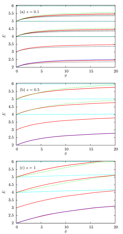
Figure 1: (a-c) Low-energy spectrum for $N=2$ interacting bosons trapped in a 2D isotropic harmonic potential depending on the interaction strength $g$ for different values of the width $s$ of the two-body Gaussian-shaped potential. (Solid red lines) Energy of the ground state and the corresponding center-of-mass excitations. (Long-dashed pointed cyan lines) Unperturbed states. (Short-dashed pointed green lines) First relative excitation and the corresponding center-of-mass excitations. (a-c) (Blue dotted lines) Energy of the ground state computed with the variational ansatz of Eq. (33). (Black dashed lines) Analytic approximate energy levels using Eq. (17) of Ref. Doganov shown only in panel (a). Numerical results with (a) $M=200$ and $D_{2}^{200}=20100$, (b) and (c) $M=150$ and $D_{2}^{150}=11325$.

In Fig. 1, we show the low-energy spectrum for the system of two interacting identical bosons in the harmonic trap. In the figure, we compare results obtained with three different values of $s=0.1$, $0.5$ and $1$. In all cases, the energy spectrum has a number of common features.

First, in the spectrum, there are the states discussed in Sect. III.1.1, which are essentially insensitive to the interaction. In the zero range limit, these are basically states with non-zero relative angular momentum, which do not feel the contact interaction Doganov . With finite interactions but for a small range, $s=0.1$ and $0.5$, they remain mostly flat for $g$ up to $20$. For $s=1$, their energy increases slightly with $g$, deviating from the zero range prediction.

Second, the ground state energy increases linearly with $g$ for small values of $g$. Up to first order perturbation theory, the energy is given by

$$E_{0}\simeq 2+\frac{g}{\pi\left(s^{2}+2\right)}.$$ (29)

However, the ground state energy tends to saturate as $g$ is increased. For smaller values of $s$, this saturation takes place at smaller values of $g$.

Third, there are the energies coming from the relative part of the Hamiltonian with the center of mass at the ground state, i.e. $n_{\rm cm}=0$. The ground state is one of these states and there is one state of this type in each energy level with an even $N_{E}$ in the noninteracting limit.

Finally, the spectrum also contains center-of-mass excitations Busch , which are easily recognized as constant energy shifts independent of $g$ with respect to states with $n_{\rm cm}=0$.

For comparison, we depict also the approximate values of Doganov in panel (a) of Fig. 1. As reported in Ref. Doganov , their approximate solution – which is not variational – starts to deviate from the exact numerical results at values of $g\simeq 4$. The approximation gives, however, a fairly good overall picture of the low-lying two-particle spectrum.

IV.2 Degeneracy for the interacting two-boson system

We can label the states with three quantum numbers. Two are the ones corresponding to the center of mass, $n_{\rm cm}$ and $m_{\rm cm}$, and the other is a new quantum number, $\nu_{r}$, that labels the nondegenerate eigenstates of the relative part of the Hamiltonian. We can write those states as

$$\Psi(R,\varphi_{R},r)=\chi_{n_{\rm cm},m_{\rm cm}}(\sqrt{2},R,\varphi_{R})f_{\nu_{r}}(r),$$ (30)

where $\chi_{n_{\rm cm},m_{\rm cm}}(\sqrt{2},R,\varphi_{R})$ is given in Sect. III and $f_{\nu_{r}}(r)$ is the relative wave function, that depends on $g$ and $s$. The other states that are in the spectrum are the unperturbed ones (almost unaffected by the interaction). Their degeneracy is given in Sec. III. The states of Eq. (30), for a given $\nu_{r}$, are degenerate with degeneracy given by the 2D harmonic oscillator of the center-of-mass part, i.e., their degeneracy is $n_{\rm cm}+1$. From each noninteracting energy level with even $N_{E}$, a state with a new $\nu_{r}$ arises, and its center-of-mass excitations appear in higher energy levels with degeneracy $n_{\rm cm}+1$, too. To sum up, the ground state is nondegenerate. The first excited state is two-degenerate and the two states are the two possible center-of-mass excitations of the ground state. The third noninteracting energy manifold (6 states with $E(g=0)=4$) splits in three: 1) three center-of-mass excitations of the ground state, 2) two unperturbed states and, 3) the new relative state with quantum numbers $n_{\rm cm}=0$, $m_{\rm cm}=0$ and $\nu_{r}=1$ with $E(g=2)=4.21$. We give the degeneracy and the quantum numbers of the low-energy states in Table 4.

$n_{\rm cm}$	$n_{r}$	$m_{\rm cm}$	$m_{r}$	$\nu_{r}$	$E(g=0)$	$E(g=2)$	$d_{int}(g=2)$
0	-	0	0	1	2	2.23	1
1	-	-1	0	1	3	3.23
1	-	1	0	1	3	3.23	2
2	-	-2	0	1	4	4.23
2	-	0	0	1	4	4.23	3
2	-	2	0	1	4	4.23
0	-	0	0	2	4	4.21	1
0	2	0	-2	-	4	4.00
0	2	0	2	-	4	4.00	2
3	-	-3	0	1	5	5.23
3	-	-1	0	1	5	5.23
3	-	1	0	1	5	5.23	4
3	-	3	0	1	5	5.23
1	-	-1	0	2	5	5.21
1	-	1	0	2	5	5.21	2
1	2	-1	-2	-	5	5.00
1	2	1	-2	-	5	5.00
1	2	-1	2	-	5	5.00	4
1	2	1	2	-	5	5.00

Table 4: Quantum numbers, energy in the noninteracting limit, energy at $g=2$ and degeneracy, for the low-energy levels of a system of two interacting identical bosons trapped in a 2D isotropic harmonic potential. The energies are in units of $\hbar\omega$ and the ones with $g=2$ correspond to a vertical cut in Fig. 1 panel (b), $s=0.5$.

IV.3 Three and four-boson energy spectra

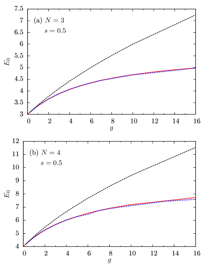
Figure 2: Ground-state energy for (a) N=3 and (b) N=4 interacting bosons trapped in a 2D isotropic harmonic potential depending on the interaction strength $g$. (Red solid line) computed numerically with ARPACK and (a) $M=80$ and (b) $M=50$, (blue dotted line) computed with the variational many-body wave function of Eq. (33), (black dashed line) computed with a Gaussian variational ansatz, Eq. (31).

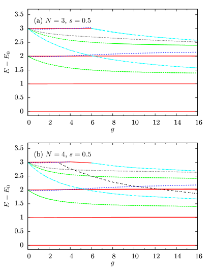
Figure 3: Low-energy spectrum for (a) $N=3$ and (b) $N=4$ interacting bosons trapped in a 2D isotropic harmonic potential depending on the interaction strength $g$. (Red solid lines) Energy of the ground state, (green dashed lines) the first, (blue dotted lines) the second, (cyan dashed-dotted lines) the third, (grey triple-dotted lines) the fourth and (black double-dotted lines) the fifth relative excitations and, respectively, their center-of-mass excitations in the same kind of line and color. The number of modes that we have used is (a) $M=80$ and (b) $M=50$, that corresponds to Hilbert spaces of dimension $D_{3}^{80}=88560$ and $D_{4}^{50}=292825$, respectively.

Our exact diagonalization scheme allows us to obtain the lowest part of the many-body spectrum for systems of up to $4$ bosons with good accuracy, up to values of $g\simeq 20$. In Fig. 2 we report the ground state energy for $N=3$ and $N=4$ bosons compared with a simple mean-field variational ansatz using the following wave function,

$$\Psi(\vec{x}_{1},\,...\,,\vec{x}_{N})=\left(\frac{\alpha}{\pi}\right)^{\frac{N}{2}}\prod_{i=1}^{N}e^{-\frac{1}{2}\alpha\vec{x}^{2}_{i}},$$ (31)

and finding the optimum $\alpha^{*}$ that minimizes the energy

$$E_{0}(\alpha) = \int_{-\infty}^{\infty}d\vec{x}_{1}\,...\,d\vec{x}_{N}\,\Psi^{*}(\vec{x}_{1},\,...\,,\vec{x}_{N})H\Psi(\vec{x}_{1},\,...\,,\vec{x}_{N})$$ (32)

$$= N\left(\frac{\alpha}{2}+\frac{1}{2\alpha}\right)+\frac{gN(N-1)\alpha}{2\pi\left(\alpha s^{2}+2\right)}.$$

As expected, this mean-field ansatz captures well the behaviour of the ground state of the system for small values of $g$. For $g\simeq 2$, however, we already observe substantial deviations, with the meanfield prediction overstimating the ground state energy considerably. In particular, as we will see below, the system develops strong beyond-mean-field correlations as $g$ is increased.

In addition, we introduce a two-body-correlated variational many-body ansatz of Jastrow type Jastrow ,

$$\Psi(\vec{x}_{1},\,...\,,\vec{x}_{N})=\left(\frac{\alpha}{\pi}\right)^{\frac{N}{2}}\prod_{i=1}^{N}e^{-\frac{1}{2}\alpha\vec{x}^{2}_{i}}\prod_{j<i}^{N}\left(1-ae^{-b(\vec{x}_{i}-\vec{x}j)^{2}}\right),$$ (33)

where $\alpha$, $a$ and $b$ are the variational parameters. We observe in Fig. 2 that the energies computed with this ansatz, using standard Monte-Carlo methods, are very close, and some times even below, the exact diagonalization ones. To improve the latter, one needs to enlarge the Hilbert space (larger $M$) to get a slightly lower upper bound. In principle, the exact diagonalization procedure for a given $M$ provides an upper bound for the ground state and each excited state. In the next section, we explain the physical interpretation of the variational parameters and discuss how well the ansatz captures the physics of the problem.

The low-energy spectrum for $N=3$ and $N=4$ at smaller values of $g$ is fairly similar. This is not unexpected as the degenerate manifolds are the same irrespective of the number of particles, see Sect. III.2. The first excited state is a center-of-mass excitation, the Kohn mode, as seen clearly in the excitation spectra shown in Fig. 3.

Even for $g$ up to $16$, the low-energy spectra for $N=3$ and $N=4$ are quite similar. The overall picture is qualitatively the same for both cases, although for $N=4$ there are extra levels crossing. In Fig. 3 panel (b), there is a level that starts crossing the highest energy level depicted at $g\simeq 3$. This line in the spectrum comes from the fourth excited level in the noninteracting limit and is also expected to appear for systems with more particles, e.g. $N=5$. It arises from the existence of a degenerate kind of states that are found only for $N\geq 4$, as it is explained in Sect. III.

IV.4 Degeneracy for the interacting three and four-boson systems

One major difference for more than two particles, is that we do not find states not affected by the interaction. Moreover, the degeneracy of the eigenfunctions of the relative part of the Hamiltonian is not $1$. Therefore, the states cannot be uniquely characterized by $\nu_{r}$. However, we can identify the states that are center-of-mass excitations of lower energy states. In Fig. 3, in both panels, for example, for $g=1$, we know the degeneracy of all the energy levels and we can identify them. The ground state is nondegenerate. As we have said before, the first excited state is a center-of-mass excitation, with degeneracy 2. The second excited state decomposes in three states corresponding to the next center-of-mass excitations of the ground state, there are two degenerate states corresponding to a relative excitation, and finally a different relative excitation. The third excited energy level in the noninteracting limit splits when $g$ is increased in the next center-of-mass excitations of the states of the previous level, i.e., four center-of-mass excitations of the ground state, four center-of-mass excitations of the previous two-degenerate relative excited states, and two more degenerate states corresponding to two center-of-mass excitations of the single-degenerate relative energy level that appeared in the second excited state when $g$ was increased. Moreover, there are two pairs of different relative excited states that split from the noninteracting third energy level. This behaviour is the same independently of $N$ for $g$ sufficiently small, for instance, for $N=4$ up to $g=3$, where there is the previous discussed crossing of levels.

IV.5 $N$-boson energies up to first order in perturbation theory

Using the analytic expressions of the integrals of the interaction that are given in Appendix C, we compute the energies of the first three energy levels in first order perturbation theory. For the ground state of the system, the energy is given by

$$E_{0}\simeq N+g\frac{N(N-1)}{2\pi\left(s^{2}+2\right)}.$$ (34)

The next level has energy

$$E_{1}\simeq N+1+g\frac{N(N-1)}{2\pi\left(s^{2}+2\right)}.$$ (35)

The third energy level splits in three, in the way that is discussed in the previous section that is also valid for $N$ bosons, with energies

$$E_{2_{1}}\simeq N+2+g\frac{N(N-1)}{2\pi\left(s^{2}+2\right)},$$ (36)

$$E_{2_{2}}\simeq N+2+g\frac{N\left(N(2+s^{2})^{2}-s^{2}(8+s^{2})-8\right)}{2\pi\left(s^{2}+2\right)^{3}},$$ (37)

$$E_{2_{3}}\simeq N+2+g\frac{N\left(N(2+s^{2})^{2}-s^{2}(8+s^{2})-4\right)}{2\pi\left(s^{2}+2\right)^{3}}.$$ (38)

The similarity in the energy difference, $E-E_{0}$, for the case of $N=3$ and $N=4$ plotted in Fig. 3 for a small $g$ can be understood using the previous expressions. The corresponding excitation energies are, in this approximation,

$$E_{1}-E_{0}=1,$$ (39)

$$E_{2_{1}}-E_{0}=2,$$ (40)

$$E_{2_{2}}-E_{0}=2-g\frac{2N\left(1+s^{2}\right)}{\pi\left(s^{2}+2\right)^{3}},$$ (41)

$$E_{2_{3}}-E_{0}=2-g\frac{2Ns^{2}}{\pi\left(s^{2}+2\right)^{3}}.$$ (42)

In the first two cases, Eq. (39) and Eq. (40), we recover the first and the second center-of-mass excitations that are red solid lines in Fig. 3. The presence of the factor $N$ in the quantity $E_{2_{2}}-E_{0}$, see Eq. (41), explains why the slope of the green dashed lines is slightly bigger in absolute value for $N=4$, panel (b), than for $N=3$, panel (a), in Fig. 3 for $g\simeq 0$. This effect would be notorious when comparing the spectrum for two very different numbers of particles. Finally, we also see that the second term in $E_{2_{3}}-E_{0}$ is proportional to $N$, but in that case, for $s$ small, the second term becomes negligible. Therefore, the blue dotted lines are very close to the red solid lines in the spectra for $g\simeq 0$, as we have used $s=0.5$. In the zero-range limit, this approximation gives $E_{2_{3}}(s\rightarrow 0)=E_{2_{1}}(s\rightarrow 0)$. As the perturbative correction affects only the relative motion, the corrections to $E_{0}$, $E_{1}$ and $E_{2_{1}}$ are equal.

V Interactions and quantum correlations

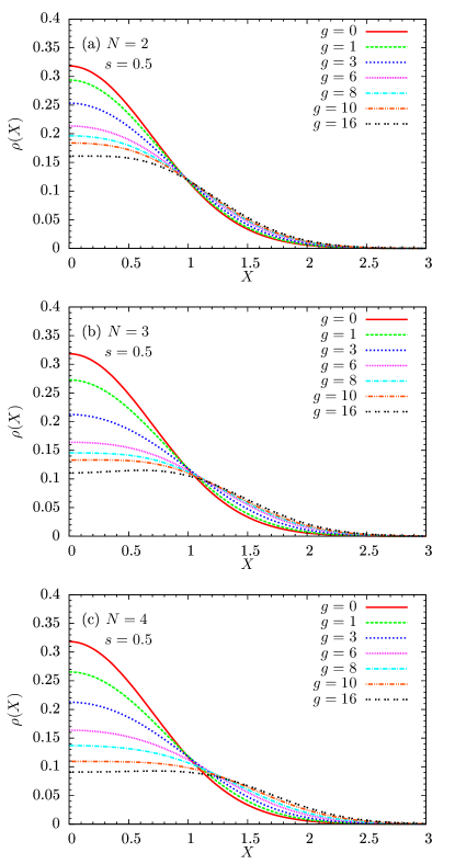
Figure 4: Density profile of the ground state for (a) $N=2$, (b) $N=3$ and (c) $N=4$ interacting bosons trapped in a 2D isotropic harmonic potential for different values of the interaction strength $g$ for a fixed range $s=0.5$. The number of modes that we have used is $M=50$, which corresponds to a Hilbert space with dimension (a) $D_{2}^{50}=1275$, (b) $D_{3}^{50}=22100$ and (c) $D_{4}^{50}=292825$.

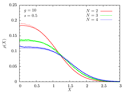
Figure 5: Density profile for $N=2$, $3$, and $4$ interacting bosons trapped in a 2D isotropic harmonic potential computed with the ground state obtained using ARPACK with $M=50$ (lines) and obtained from the variational ansatz, Eq. (33), (crosses, squares and dots) for $g=10$ and $s=0.5$.

As seen in the previous section, the ground state energy of the system for $N=2,3$ and 4 tends to saturate as we increase the strength of the atom-atom interactions. This saturation starts to occur for values $g$ for which the mean-field variational ansatz starts to deviate from the exact results. This reminds of a similar effect found in 1D systems, where the ground state evolves from mean-field to Tonks-Girardeau gas as the interaction strength is increased. In the Tonks-Girardeau limit, the atoms do avoid completely the atom-atom contact interaction by building strong correlations which in 1D are easily understood from the Bose-Fermi mapping theorem Girardeau2 . In 2D, no such mapping exist. However, we expect that the system should build suitable correlations to avoid the interaction, resulting in a saturation of the energy for increasing $g$.

For the ground state, besides the exact diagonalization method, we have also made use of a correlated variational ansatz, Eq. (33), to enlighten the discussion. The energies and properties associated to this variational ansatz are evaluated by means of Monte-Carlo methods (standard Metropolis algorithm). The physical meaning of the variational parameters is quite transparent. $\alpha$ directly affects the overall size of the cloud. The two-body Jastrow correlations are parameterized by $a$ and $b$. Two limiting cases are illustrative. If the system is fully condensed we will have $a=0$, while $a=1$ would correspond to building a zero of the wave function whenever two atoms are at the same position. $b$ affects the two-body correlation length. Thus, we expect the following behavior: for values of $g\simeq 0$ we should have $a=0$ ($b$ is thus irrelevant) and $\alpha$ close to $1$. For increasing $g$, $\alpha$ decreases to avoid the interaction by simply putting the atoms apart. As we increase $g$, two-body correlations build in, $a\neq 0$ and $\alpha$ should stop decreasing as the correlation is more efficient to separate the atoms.

Let us first discuss the density profile of the clouds, see Appendix B for definitions. In Fig. 4 we show the density profile, normalized to unity, depending on the radial coordinate $X=\sqrt{x^{2}+y^{2}}$, computed with our exact diagonalization procedure. Due to the symmetry of the trap, the density profile of the ground state does not have angular dependence, see Appendix B, Eq. (58). In panels (a), (b) and (c) we show results for $N=2$, $3$, and $4$. In all cases, with the same value of $s=0.5$. We compare densities obtained for different values of $g$.

Irrespective of $N$ we observe a number of common features. For $g=0$, the system has a Gaussian density profile which, as $g$ is increased, evolves into a profile with a flat region for $X\leq 1$ at $g\simeq 16$. As $N$ is increased, the size of the inner plateau increases, thus tending towards an homogeneous density.

The quality of our variational approach is seen in Fig. 5. We compare density profiles obtained with the exact diagonalization procedure with those obtained variationally by means of Eq. (33). As seen in the figure, the variational wave function provides a fairly accurate representation of the density profile for $N=2$, $3$, and $4$. In particular, it captures well the appearance of the plateau.

The effect of increasing the interaction among the atoms is manifold. As we have seen above, the density profile is modified and the gas becomes close to homogeneous in the inner part of the trap. This change in the density is however accompanied by a change in the correlations present in the system. Actually, the gas goes from a fully condensed state to a largely fragmented one as we increase the interaction. In Fig. (6), we depict how the condensed fraction for $N=2$, $3$, and $4$ decreases when increasing the interaction strength. For the same value of $g$, the fragmentation in the system is larger for larger number of particles.

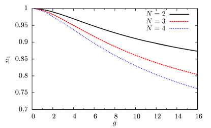
Figure 6: Condensed fractions of the ground state for (black line) $N=2$, (red-dashed line) $N=3$ and (green spotted line) $N=4$ interacting bosons trapped in a 2D isotropic harmonic potential depending on the interaction strength $g$ for a fixed range $s=0.5$. The number of modes that we have used is $M=50$ and the rest of the eigenstates of the one-body density matrix are much more smaller than the biggest one.

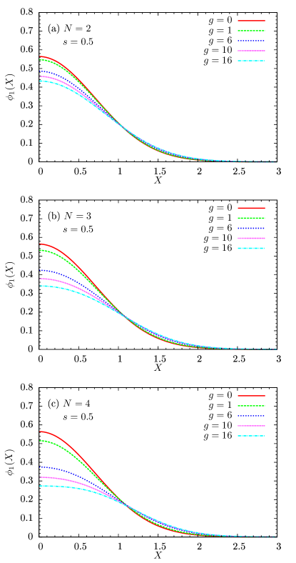
Figure 7: Single-particle eigenstate of the one-body density matrix in which the particles condense. We use Eq. (44) and the values of $C_{0}$ and $C_{1}$ computed numerically diagonalizing the one-body density matrix, Eq. (77), for different values of $g$. (a) $N=2$ bosons, (b) $N=3$ and (c) $N=4$. The fraction of condensed particles is plotted in Fig. 6. The number of modes that we have used is $M=50$, which corresponds to a Hilbert space with dimension (a) $D_{2}^{50}=1275$, (b) $D_{3}^{50}=22100$ and (c) $D_{4}^{50}=292825$.

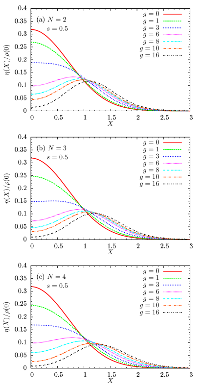
Figure 8: Probability density, $\eta(X)/\rho(0)$, of finding a particle at position $X$ once we have found one particle at the origin, $X=0$, for (a) $N=2$, (b) $N=3$ and (c) $N=4$ interacting bosons trapped in a 2D isotropic harmonic potential for different values of the interaction strength $g$ for a fixed range $s=0.5$. The number of modes that we have used is $M=50$, which corresponds to a Hilbert space with dimension (a) $D_{2}^{50}=1275$, (b) $D_{3}^{50}=22100$ and (c) $D_{4}^{50}=292825$.

The most populated eigenstate of the one-body density matrix (natural orbit), is found to have the approximate form, using the $\ket{n_{x},n_{y}}$ basis,

$$\ket{\phi_{1}}\simeq C_{0}\ket{0,0}+C_{1}\left(\ket{2,0}+\ket{0,2}\right),$$ (43)

and its wave function reads

$$\phi_{1}(X)\simeq\frac{1}{\sqrt{\pi}}e^{-\frac{X^{2}}{2}}\left(C_{0}-\sqrt{2}C_{1}\left(1-X^{2}\right)\right).$$ (44)

This natural orbit is a superposition of the two first single-particle states of the 2D harmonic oscillator with zero angular momentum, $m=0$, the state $\ket{n=0,m=0}$ and the state $\ket{n=2,m=0}$, thus the wave function has no angular dependence. For the noninteracting case, $C_{0}=1$ and $C_{1}=0$, since the particles condense in the ground state of the harmonic oscillator. When the interaction is increased, $C_{0}$ becomes smaller and $C_{1}$ starts to increase. In Fig. 7, we plot the wave function of Eq. (44) using the corresponding values of $C_{0}$ and $C_{1}$ computed for $N=2,3,4$ and different values of the interaction strength $g$.

The advent of correlations beyond mean-field ones should also become apparent when computing two-particle correlations. In particular, we can evaluate the probability of finding two particles at given positions. For simplicity we consider one of them at the origin and the second one at a distance $X$. The probability density of finding a particle in the space once we have fixed a particle at the center is given by $\eta(X)/\rho(0)$ and is normalized to unity (see Appendix B). Without interactions, the pair correlation function is proportional to the density, since the probability density for finding a particle in a particular place is not correlated with the positions of the others, see Eq. (72). In Fig. 8, we show how $\eta(X)/\rho(0)$ evolves with increasing the interaction for the systems with $N=2$, $3$, and $4$ bosons. In all cases, the central peak gets smaller when increasing the interaction, being fairly close to zero for $g\simeq 16$. This is in line with the fact that the atoms build correlations to avoid the interaction, e.g. as $g$ is increased the probability of finding two atoms at the same location decreases. In between, next to the center of the trap, the function is uniform. When the interaction is strong there is a minimum at the position of the first atom, the probability density $\eta(X)/\rho(0)$ develops a maximum corresponding to the preferred distance between particles. Increasing the number of bosons, this maximum shifts towards larger distances.

VI Summary and Conclusions

In this work, we have studied systems of a few number of bosons trapped in an isotropic 2D harmonic trap interacting by a finite-range Gaussian potential.

First, we have explored in detail the noninteracting case, paying particular attention to the degeneracies of the excitation spectrum of the system. In particular, for the $N$-boson case, we have explained how to compute the degeneracy of the low-energy states which is independent of the number of particles.

By means of a direct diagonalization of the Hamiltonian in a truncated space, we have studied the interacting system and we have computed the low-energy spectra for $N=2$, $3$, and $4$ bosons. We have also proposed a variational ansatz with two-body correlations which provides an accurate description of both the energy and the structure of the ground state in the full range of interaction considered. Center-of-mass and relative excitations are clearly identified in the spectrum. As the interaction is increased, we have shown how the ground state and all low lying states tend to saturate as a function of the interaction strength.

The effect of increasing the interaction on the ground state is twofold. On one side, the density at the center of the trap decreases becoming almost flat in the bulk of the gas, with the cloud thus becoming larger. On the other side, the atoms develop strong two-body correlations to avoid the interaction. This is achieved by building holes in the many-body wave function whenever two atoms are at the same position, as is clearly seen in the computed pair correlations and also on the explicit zeros introduced in our variational wave function. This mechanism is similar to the one present in the Tonks-Girardeau gas in 1D and is also responsible for the observed saturation of the energies of the system as we increase the interaction strength. Finally, the onset of correlations in turn produces fragmentation on the one-body density matrix, which has been shown to increase with the number of particles.

Thus, we have shown that our exact diagonalization method allows one to study interacting bosonic systems in 2D. We are presently implementing this method for spin-orbit coupled bosonic systems.

Appendix A Computation of degeneracies in the noninteracting limit

A.1 The two-boson system

We compute the degeneracy of each energy level depending on the excitation energy number, $N_{E}=E-E_{0}$, for the two-boson system with the possible states labelled using the quantum numbers of Eq. (20). First, we fix the excitation energy number, $N_{E}$, and consider it to be even. Then, the values that $n_{r}$ can take are $n_{r}=0,2,\,...\,,N_{E}$, so $n_{r}=2k$ with $k=0,1,\,...\,,N_{E}/2$. Since we have $n_{\rm cm}+n_{r}=N_{E}$, for each value of $n_{r}$ there is the corresponding $n_{\rm cm}$. Now, we count the number of states with a given $n_{r}$ with excitation energy number $N_{E}$ taking into account the degeneracy due to the quantum numbers $m_{\rm cm}$ and $m_{r}$, that is,

$$d_{N_{E},k}=(n_{\rm cm}+1)(n_{r}+1)=(N_{E}-2k+1)(2k+1).$$ (45)

Therefore, we have to sum over $k$ to find the degeneracy. The sum goes from $k=0$ to $k=N_{E}/2$ if $N_{E}$ is even and to $k=(N_{E}-1)/2$ if $N_{E}$ is odd, which can be generalized using the floor function, summing from $k=0$ to $k=\left\lfloor N_{E}/2\right\rfloor$. The degeneracy is

$$\begin{gathered}d^{b}_{N_{E}}=\sum_{k=0}^{\left\lfloor N_{E}/2\right\rfloor}(N_{E}-2k+1)(2k+1)=\\ -\frac{1}{3}\left(\left\lfloor\frac{N_{E}}{2}\right\rfloor+1\right)\\ \times\left[4{\left\lfloor\frac{N_{E}}{2}\right\rfloor}^{2}+(2-3N_{E})\left\lfloor\frac{N_{E}}{2}\right\rfloor-3(N_{E}+1)\right].\end{gathered}$$ (46)

The previous equation, Eq. (46), for $N_{E}$ even is

$$d^{b}_{N_{E}}=\frac{1}{12}\left(N_{E}+2\right)\left(N_{E}(N_{E}+4)+6\right),$$ (47)

and for $N_{E}$ odd is

$$d^{b}_{N_{E}}=\frac{1}{12}\left(N_{E}+1\right)\left(N_{E}(N_{E}+5)+6\right).$$ (48)

For the spatial fermionic states, which are the ones with $m_{r}=$ odd and antisymmetric upon exchanging particles $1$ and $2$, we compute the degeneracy analogously, using that $n_{r}=$ odd,

$$\begin{gathered}d^{f}_{N_{E}}=\sum_{k=0}^{\left\lfloor N_{E}/2\right\rfloor}(N_{E}-2k)(2k+2)=\\ -\frac{1}{3}\left(\left\lfloor\frac{N_{E}}{2}\right\rfloor+1\right)\\ \times\left[4{\left\lfloor\frac{N_{E}}{2}\right\rfloor}^{2}+(8-3N_{E})\left\lfloor\frac{N_{E}}{2}\right\rfloor-6N_{E}\right].\end{gathered}$$ (49)

A.1.1 Unperturbed energy states

We are also interested in knowing the number of states in each energy level with $m_{r}\neq 0$. We compute this number of states subtracting from the total number of degenerate states, $d^{b}_{N_{E}}$, the ones with $m_{r}=0$, that is,

$$\begin{gathered}d^{U}_{N_{E}}=d^{b}_{N_{E}}-\sum_{k=0}^{\left\lfloor N_{E}/2\right\rfloor}(N_{E}-2k+1)\\ =\left(-\frac{4}{3}\left\lfloor\frac{N_{E}}{2}\right\rfloor+N_{E}+\frac{1}{3}\right)\left\lfloor\frac{N_{E}}{2}\right\rfloor\left(\left\lfloor\frac{N_{E}}{2}\right\rfloor+1\right),\end{gathered}$$ (50)

where we have used Eq. (46). As before, we can separate the case with $N_{E}$ even,

$$d^{U}_{N_{E}}=\frac{1}{12}(N_{E}+2)(N_{E}+1)N_{E},$$ (51)

and the case with $N_{E}$ odd,

$$d^{U}_{N_{E}}=\frac{1}{12}(N_{E}+3)(N_{E}+1)(N_{E}-1).$$ (52)

Appendix B Computation of the density profile, the pair correlation function and the condensed fraction

B.1 The density profile

B.1.1 First-quantized density operator

For a system of $N$ particles, the density operator in first quantization, normalized to unity, is defined as

$$\hat{\rho}(\vec{x})\equiv\frac{1}{N}\sum_{i=1}^{N}\delta({\vec{x}-\vec{x}_{i}}).$$ (53)

Therefore, the density profile for a given state of a system of $N$ identical bosons, $\Psi(\vec{x}_{1},\,...\,,\vec{x}_{N})$, would be

$$\begin{gathered}\rho(\vec{x})=\frac{1}{N}\sum_{i=1}^{N}\int d\vec{x}_{1}\,...\,d\vec{x}_{N}\,\delta({\vec{x}-\vec{x}_{i}})\left|\Psi(\vec{x}_{1},...\,,\vec{x}_{N})\right|^{2}\\ =\int d\vec{x}_{2}\,...\,d\vec{x}_{N}\,\left|\Psi(\vec{x},\vec{x}_{2}...,\vec{x}_{N})\right|^{2}.\end{gathered}$$ (54)

In particular, for a two-boson system in 2D, the previous equation reduces to

$$\rho(x,y)=\int_{-\infty}^{\infty}dx_{2}\int_{-\infty}^{\infty}dy_{2}\left|\Psi\left(x,y,x_{2},y_{2}\right)\right|^{2}.$$ (55)

We compute the density profile for the general interacting case, in the harmonic trap, for the ground state of the system as

$$\rho(x,y)=\int_{-\infty}^{\infty}dx_{2}\int_{-\infty}^{\infty}dy_{2}\frac{2}{\pi}e^{-\frac{1}{2}\left(\vec{x}+\vec{x}_{2}\right)^{2}}\left|f\left(|\vec{x}-\vec{x}_{2}|\right)\right|^{2},$$ (56)

where we have made use of the explicit form of the many-body wave function of the ground state,

$$\Psi\left(\vec{x}_{1},\vec{x}_{2}\right)=\sqrt{\frac{2}{\pi}}e^{-\frac{1}{4}\left(\vec{x}_{1}+\vec{x}_{2}\right)^{2}}f\left(\left|\vec{x}_{1}-\vec{x}_{2}\right|\right).$$ (57)

This way of writing the wave function of the ground state is equivalent to separate the center-of-mass part from the relative part. Using the change of variables $\vec{r}=\vec{x}-\vec{x}_{2}$ and polar coordinates in Eq. (56), we express the density as

$$\begin{gathered}\rho(x,y)=\frac{2}{\pi}e^{-2(x^{2}+y^{2})}\int_{0}^{\infty}r\,dr\,e^{-\frac{r^{2}}{2}}\left|f\left(r\right)\right|^{2}\\ \times\int_{0}^{2\pi}d\varphi\,e^{-2r\left(x\cos\varphi+y\sin\varphi\right)}=4e^{-2(x^{2}+y^{2})}\\ \times\int_{0}^{\infty}r\,dr\,e^{-\frac{r^{2}}{2}}\left|f\left(r\right)\right|^{2}\mathcal{I}_{0}\left(2r\sqrt{x^{2}+y^{2}}\right).\end{gathered}$$ (58)

We have used that

$$\int_{0}^{2\pi}d\varphi\,e^{A\cos\varphi+B\sin\varphi}=2\pi\,\mathcal{I}_{0}\left(\sqrt{A^{2}+B^{2}}\right),$$ (59)

where $\mathcal{I}_{0}$ is a modified Bessel function. Notice that, as we would expect, in Eq. (58) we have demonstrated that the density only depends on the radial coordinate $X\equiv\sqrt{x^{2}+y^{2}}$, and we can rewrite that equation as

$$\rho(X)=4e^{-2X^{2}}\int_{0}^{\infty}rdr\,e^{-\frac{r^{2}}{2}}\left|f\left(r\right)\right|^{2}\mathcal{I}_{0}\left(2rX\right).$$ (60)

This result is valid not only for our Gaussian-shaped potential but also for any potential dependent only on the modulus of the relative coordinate. In these other cases, the explicit form of the interaction defines the relative wave function $f(r)$. In the noninteracting case, we can compute the integral analytically, by substituting the explicit form of $f_{0}(r)$,

$$f_{0}(r)=\frac{1}{\sqrt{2\pi}}e^{-\frac{r^{2}}{4}},$$ (61)

and we recover the known result,

$$\begin{gathered}\rho_{0}(X)=\frac{2}{\pi}e^{-2X^{2}}\int_{0}^{\infty}rdr\,e^{-r^{2}}\mathcal{I}_{0}\left(2rX\right)\\ =\frac{1}{\pi}e^{-X^{2}}=\left|\varphi_{0}(X)\right|^{2},\end{gathered}$$ (62)

where $\varphi_{0}(X)$ is the wave function of the single-particle ground state of the 2D harmonic oscillator. The previous result, $\rho_{0}(X)=\left|\varphi_{0}(X)\right|^{2}$, is also valid for the case of $N$ noninteracting bosons in the 2D harmonic potential, since the many-body wave function factorizes, $\Psi_{0}(\vec{x}_{1},\vec{x}_{2}...,\vec{x}_{N})=\varphi_{0}(\vec{x}_{1})\,...\,\varphi_{0}(\vec{x}_{N})$. We recover the previous result replacing the factorized wave function into Eq. (54).

B.1.2 Second-quantized density operator

For our numerical computations, we make use of the second-quantized form of the density operator,

$$\hat{\rho}=\frac{1}{N}\sum_{i,j=1}^{M}\hat{a}^{\dagger}_{i}\hat{a}_{j}\psi^{*}_{i}(\vec{x})\psi_{j}(\vec{x}).$$ (63)

For a state written in our Fock basis, Eq. (11), as

$$\ket{\Psi}=\sum_{k=1}^{D^{M}_{N}}\alpha_{k}\ket{k},$$ (64)

where the index $k$ labels each state of the basis, $\ket{k}=\ket{n_{1},\,...\,,n_{M}}$, the density profile is computed as

$$\rho(\vec{x})=\frac{1}{N}\sum_{k^{\prime},k=1}^{D^{M}_{N}}\sum_{i,j=1}^{M}\psi^{*}_{i}(\vec{x})\psi_{j}(\vec{x})\alpha^{*}_{k^{\prime}}\alpha_{k}\bra{k^{\prime}}\hat{a}^{\dagger}_{i}\hat{a}_{j}\ket{k},$$ (65)

where $\psi_{i}(\vec{x})$ are the single-particle eigenstates of the 2D harmonic oscillator.

B.2 The pair correlation function

The pair correlation operator, normalized to unity, for a system of $N$ particles reads

$$\hat{\eta}(\vec{x},\vec{x}^{\prime})\equiv\frac{1}{N(N-1)}\sum_{i=1}^{N}\sum_{j\neq i}^{N}\delta(\vec{x}-\vec{x}_{i})\delta(\vec{x}^{\prime}-\vec{x}_{j}),$$ (66)

from which we obtain the pair correlation function for a state of the $N$-boson system, $\Psi(\vec{x}_{1},\,...\,,\vec{x}_{N})$, as

$$\begin{gathered}\eta(\vec{x},\vec{x}^{\prime})=\frac{1}{N(N-1)}\sum_{i=1}^{N}\sum_{j\neq i}^{N}\int d\vec{x}_{1}\,...\,d\vec{x}_{N}\\ \times\delta(\vec{x}-\vec{x}_{i})\delta(\vec{x}^{\prime}-\vec{x}_{j})\left|\Psi(\vec{x}_{1},\,...\,,\vec{x}_{N})\right|^{2}\\ =\int d\vec{x}_{3}\,...\,d\vec{x}_{N}\left|\Psi(\vec{x},\vec{x}^{\prime},\vec{x}_{3}\,...\,,\vec{x}_{N})\right|^{2}.\end{gathered}$$ (67)

For the particular case of the ground state of two bosons in 2D, we have

$$\eta\left(\vec{x},\vec{x}^{\prime}\right)=\left|\Psi\left(\vec{x},\vec{x}^{\prime}\right)\right|^{2},$$ (68)

where $\Psi\left(\vec{x},\vec{x}^{\prime}\right)$ is the corresponding wave function, Eq. (57). For the noninteracting case, in the harmonic trap, we know the function of the relative part, Eq. (61). In that case, the pair correlation function is

$$\eta_{0}\left(\vec{x},\vec{x}^{\prime}\right)=\frac{1}{\pi^{2}}e^{-\vec{x}^{2}}e^{-\vec{x}^{\prime 2}}=\left|\varphi_{0}(\vec{x})\right|^{2}\left|\varphi_{0}(\vec{x}^{\prime})\right|^{2}.$$ (69)

The last result is also valid for the system of $N$ bosons, because then we can factorize, $\Psi_{0}(\vec{x}_{1},\vec{x}_{2}...,\vec{x}_{N})=\varphi_{0}(\vec{x}_{1})\,...\,\varphi_{0}(\vec{x}_{N})$, and replace the wave function into Eq. (67) in order to find the same result.

Now, we fix one particle at the origin, and compute the function

$$\eta\left(x,y\right)\equiv\eta(\vec{x},\vec{0})=\frac{2}{\pi}e^{-\frac{1}{2}\left(x^{2}+y^{2}\right)}\left|f(\sqrt{x^{2}+y^{2}})\right|^{2}.$$ (70)

Notice that the previous function depends only on the radial coordinate $X\equiv\sqrt{x^{2}+y^{2}}$, so we can write

$$\eta(X)=\frac{2}{\pi}e^{-\frac{1}{2}X^{2}}\left|f(X)\right|^{2}.$$ (71)

Again, for the noninteracting case we have an analytical expression for the previous function, that reads

$$\eta_{0}(X)=\frac{1}{\pi^{2}}e^{-X^{2}},$$ (72)

and is proportional to the density, Eq. (62).

The probability density of finding a particle in the space once we have found a particle at the origin is given by the quantity $\eta(X)/\rho(0)$. We verify its normalization to unity in the general case,

$$\int d\vec{x}\,\frac{\eta(\vec{x},\vec{0})}{\rho(\vec{0})}=\frac{\int d\vec{x}\,d\vec{x}_{3}\,...\,d\vec{x}_{N}\left|\Psi(\vec{x},\vec{0},\vec{x}_{3}\,...\,,\vec{x}_{N})\right|^{2}}{\int d\vec{x}_{2}\,...\,d\vec{x}_{N}\left|\Psi(\vec{0},\vec{x}_{2},\vec{x}_{3}\,...\,,\vec{x}_{N})\right|^{2}}=1,$$ (73)

where we have used that all the particles are identical, Eq. (54) and Eq. (67).

B.2.1 Second-quantized pair correlation operator

The second-quantized form of the pair correlation operator is

$$\hat{\eta}=\frac{1}{N(N-1)}\sum_{i,j,p,q=1}^{M}\hat{a}^{\dagger}_{i}\hat{a}^{\dagger}_{p}\hat{a}_{j}\hat{a}_{q}\psi^{*}_{i}(\vec{x})\psi^{*}_{p}(\vec{x}^{\prime})\psi_{j}(\vec{x})\psi_{q}(\vec{x}^{\prime}).$$ (74)

For a state written in our Fock basis, Eq. (11), as

$$\ket{\Psi}=\sum_{k=1}^{D^{M}_{N}}\alpha_{k}\ket{k},$$ (75)

where the index $k$ labels each state of the basis, $\ket{k}=\ket{n_{1},\,...\,,n_{M}}$, the pair correlation function is computed as

$$\begin{gathered}\eta(\vec{x},\vec{x}^{\prime})=\frac{1}{N(N-1)}\sum_{i,j,p,q=1}^{M}\psi^{*}_{i}(\vec{x})\psi^{*}_{p}(\vec{x}^{\prime})\psi_{j}(\vec{x})\psi_{q}(\vec{x}^{\prime})\\ \times\sum_{k^{\prime},k=1}^{D^{M}_{N}}\alpha^{*}_{k^{\prime}}\alpha_{k}\bra{k^{\prime}}\hat{a}^{\dagger}_{i}\hat{a}^{\dagger}_{p}\hat{a}_{j}\hat{a}_{q}\ket{k},\end{gathered}$$ (76)

where $\psi_{i}(\vec{x})$ are the single-particle eigenstates of the 2D harmonic oscillator.

B.3 The condensed fraction

The degree of condensation is characterized using the one-body density matrix,

$$\rho_{i,j}^{\ket{\Psi}}\equiv\frac{1}{N}\bra{\Psi}\hat{a}^{\dagger}_{i}\hat{a}_{j}\ket{\Psi},$$ (77)

where, $i,j=1,\,...\,,M$. Diagonalizing this matrix, its eigenvalues $n_{i}$ are computed, which are the occupations of the corresponding singe-particle eigenstates $\ket{\phi_{i}}$. The state $\ket{\Psi}$ is fully condensed when $\ket{\Psi}=\ket{\phi_{1}}^{\otimes N}$ and then, the one-body density matrix has only a single nonzero eigenvalue, $n_{1}=1$. If there is fragmentation in the system, the highest eigenvalue $n_{1}<1$, due to the normalization, $\sum_{i=1}^{M}n_{i}=1$.

Appendix C Computation of the integrals of interaction for the second-quantized Hamiltonian

We make an effort to find an analytic expression for the integrals of the interaction part because, in this way, we avoid computing a lot of 4-dimensional integrals numerically, which would mean needing more computational time in order to achieve a good precision before any other calculation. With our method, we have a fast and accurate subroutine that computes $V_{i,j,k,l}$.

In order to compute the integrals, we write explicitly the single-particle wave functions corresponding to the $i^{th}$ eigenstate of the single-particle Hamiltonian,

$$\psi_{i(n_{x},n_{y})}(x,y)=N_{n_{x}}N_{n_{y}}H_{n_{x}}(x)H_{n_{y}}(y)e^{-\frac{x^{2}+y^{2}}{2}},$$ (78)

with $H_{n}(x)$ the Hermite polynomials and the normalization constant

$$N_{n}=\left(\frac{1}{\sqrt{\pi}2^{n}n!}\right)^{1/2}.$$ (79)

The Hermite polynomials are written in series representation as

$$H_{n}(x)=\sum_{m=0}^{\left\lfloor n/2\right\rfloor}\frac{n!(-1)^{m}2^{n-2m}}{m!(n-2m)!}x^{n-2m},$$ (80)

where $\left\lfloor n/2\right\rfloor$ indicates the floor function of $n/2$. We replace Eq. (78) into Eq. (9) in order to obtain

$$V_{i,j,k,l}=\frac{1}{\pi s^{2}}\prod_{i=1}^{4}N_{n_{xi}}N_{n_{yi}}I_{xx^{\prime}}I_{yy^{\prime}},$$ (81)

with

$$\begin{split}I_{xx^{\prime}}&=\int_{-\infty}^{\infty}dx^{\prime}H_{n_{x2}}(x^{\prime})H_{n_{x3}}(x^{\prime})e^{-A{x^{\prime}}^{2}}\\ &\times\int_{-\infty}^{\infty}dxH_{n_{x1}}(x)H_{n_{x4}}(x)e^{-Ax^{2}+Bx}\\ &=\int_{-\infty}^{\infty}dx^{\prime}H_{n_{x2}}(x^{\prime})H_{n_{x3}}(x^{\prime})e^{-A{x^{\prime}}^{2}}I_{x}(x^{\prime}),\end{split}$$ (82)

with the definitions

$$A\equiv 1+\frac{1}{s^{2}},$$ (83)

$$B\equiv\frac{2x^{\prime}}{s^{2}},$$ (84)

and analogously for $I_{yy^{\prime}}$. Now, we use the series representation of the Hermite polynomials, Eq. (80), to compute the integral $I_{x}(x^{\prime})$,

$$\begin{gathered}I_{x}(x^{\prime})=\sum_{k_{1}=0}^{\left\lfloor n_{x1}/2\right\rfloor}\sum_{k_{4}=0}^{\left\lfloor n_{x4}/2\right\rfloor}\frac{n_{x1}!n_{x4}!(-1)^{k_{1}+k_{4}}2^{Q}}{k_{1}!k_{4}!(n_{x1}-2k_{1})!(n_{x4}-2k_{4})!}\\ \times\int_{-\infty}^{\infty}x^{Q}e^{-Ax^{2}+Bx}dx\\ =\sum_{k_{1}=0}^{\left\lfloor n_{x1}/2\right\rfloor}\sum_{k_{4}=0}^{\left\lfloor n_{x4}/2\right\rfloor}\frac{n_{x1}!n_{x4}!(-1)^{k_{1}+k_{4}}2^{Q}}{k_{1}!k_{4}!(n_{x1}-2k_{1})!(n_{x4}-2k_{4})!}\\ \times\,i^{-Q}A^{-\frac{Q+1}{2}}\sqrt{\pi}e^{\frac{B^{2}}{4A}}U\left(-\frac{Q}{2};\frac{1}{2};\frac{-B^{2}}{4A}\right)\\ =\sqrt{\frac{\pi}{A}}e^{\frac{B^{2}}{4A}}\sum_{k_{1}=0}^{\left\lfloor n_{x1}/2\right\rfloor}\sum_{k_{4}=0}^{\left\lfloor n_{x4}/2\right\rfloor}\sum_{m=0}^{\left\lfloor Q/2\right\rfloor}\frac{n_{x1}!n_{x4}!}{k_{1}!k_{4}!(n_{x1}-2k_{1})!}\\ \times\frac{(-1)^{k_{1}+k_{4}}Q!}{(n_{x4}-2k_{4})!m!(Q-2m)!A^{Q-m}}B^{Q-2m},\end{gathered}$$ (85)

where $U\left(-\frac{Q}{2};\frac{1}{2};\frac{-B^{2}}{4A}\right)$ is a confluent hypergeometric function of the second kind that we have expressed in series and $Q\in\mathbb{N}$ is defined as

$$Q\equiv n_{x1}+n_{x4}-2k_{1}-2k_{4}.$$ (86)

The next step is computing the integral in Eq. (82) by replacing the explicit form of $I_{x}(x^{\prime})$, Eq. (85). First, we notice that depending on the parity of the integrand, the integral will be zero since we integrate in a symmetric interval. The possible situations are

$$\begin{cases}I_{xx^{\prime}}=0&n_{x1}+n_{x2}+n_{x3}+n_{x4}\,\,odd\\ I_{xx^{\prime}}\neq 0&n_{x1}+n_{x2}+n_{x3}+n_{x4}\,\,even.\end{cases}$$ (87)

In the second case, we compute the integral replacing again the Hermite polynomials by their series representation and substituting (85) into (82),

$$\begin{gathered}I_{xx^{\prime}}=\int_{-\infty}^{\infty}dx^{\prime}H_{n_{x2}}(x^{\prime})H_{n_{x3}}(x^{\prime})e^{-A{x^{\prime}}^{2}}I_{x}(x^{\prime})\\ =\sum_{k_{1}=0}^{\left\lfloor n_{x1}/2\right\rfloor}\sum_{k_{2}=0}^{\left\lfloor n_{x2}/2\right\rfloor}\sum_{k_{3}=0}^{\left\lfloor n_{x3}/2\right\rfloor}\sum_{k_{4}=0}^{\left\lfloor n_{x4}/2\right\rfloor}\sum_{m=0}^{\left\lfloor Q/2\right\rfloor}\prod_{i=1}^{4}\frac{n_{xi}!}{k_{i}!(n_{xi}-2k_{i})!}\\ \times\sqrt{\frac{\pi}{A}}\frac{Q!(-1)^{\sum_{j=1}^{4}k_{j}}2^{Q^{\prime}}}{m!(Q-2m)!A^{Q-m}s^{2Q-4m}}\int_{-\infty}^{\infty}{x^{\prime}}^{Q^{\prime}}e^{-A^{\prime}{x^{\prime}}^{2}}dx^{\prime}\\ =\sum_{k_{1}=0}^{\left\lfloor n_{x1}/2\right\rfloor}\sum_{k_{2}=0}^{\left\lfloor n_{x2}/2\right\rfloor}\sum_{k_{3}=0}^{\left\lfloor n_{x3}/2\right\rfloor}\sum_{k_{4}=0}^{\left\lfloor n_{x4}/2\right\rfloor}\sum_{m=0}^{\left\lfloor Q/2\right\rfloor}\prod_{i=1}^{4}\frac{n_{xi}!}{k_{i}!(n_{xi}-2k_{i})!}\\ \times\sqrt{\frac{\pi}{A}}\frac{Q!(-1)^{\sum_{j=1}^{4}k_{j}}2^{Q^{\prime}}A^{\prime-\frac{Q^{\prime}+1}{2}}\Gamma\left(\frac{Q^{\prime}+1}{2}\right)}{m!(Q-2m)!A^{Q-m}s^{2Q-4m}},\end{gathered}$$ (88)

with the definitions

$$A^{\prime}\equiv A-\frac{1}{As^{4}},$$ (89)

$$Q^{\prime}\equiv\sum_{i=1}^{4}\left(n_{xi}-2k_{i}\right)-2m.$$ (90)

The expression is analogous for $I_{yy^{\prime}}$ and all the sums that appear are finite and have few terms when $n_{xi}$ are small. Now, knowing the form of $I_{xx^{\prime}}$ and $I_{yy^{\prime}}$ we have $V_{i,j,k,l}$. Moreover, many of the integrals are zero

$$\begin{cases}V_{i,j,k,l}=0&\sum_{i=1}^{4}n_{xi}\,\,odd\,\,\,or\,\,\,\sum_{i=1}^{4}n_{yi}\,\,odd\\ V_{i,j,k,l}\neq 0&\sum_{i=1}^{4}n_{xi}\,\,even\,\,\,and\,\,\,\sum_{i=1}^{4}n_{yi}\,\,even,\end{cases}$$ (91)

and we also take profit from the symmetries of $I_{xx}(n_{x1},n_{x2},n_{x3},n_{x4})$, which verifies

$$\begin{gathered}I_{xx}(n_{x1},n_{x2},n_{x3},n_{x4})=I_{xx}(n_{x4},n_{x2},n_{x3},n_{x1})\\ =I_{xx}(n_{x1},n_{x3},n_{x2},n_{x4})=I_{xx}(n_{x4},n_{x3},n_{x2},n_{x1}).\end{gathered}$$ (92)

Therefore, we are computing four integrals at the same time.

References

- (1) W. S. Bakr, A. Peng, M. E. Tai, R. Ma, J. Simon, J. I. Gillen, S. Fölling, L. Pollet, and M. Greiner, Science 329, 547 (2010).
- (2) J. F. Sherson, C. Weitenberg, M. Endres, M. Cheneau, I. Bloch, and S. Khur, Nature467, 68 (2010).
- (3) G. Zürn, F. Serwane, T. Lompe, A. N. Wenz, M. G. Ries, J. E. Bohn, and S. Jochim, Phys. Rev. Lett. 108, 075303 (2012).
- (4) R. Islam, R. Ma, P. M. Preiss, M. E. Tai, A. Lukin, M. Rispoli, and M. Greiner, Nature 528, 77 (2015).
- (5) M. Girardeau, J. Math. Phys. 1, 516 (1960).
- (6) B. Paredes, A. Widera, V. Murg, O. Mandel, S. Fölling, I. Cirac, G. V. Shlyapnikov, T. W. Hänsch, and I. Bloch, Nature 429, 277 (2004).
- (7) T. Kinoshita, T. Wenger, and D. S. Weiss, Science 305, 1125 (2004).
- (8) G. Pupillo, A. M. Rey, C. J. Williams, and C. W. Clark, New J. Phys. 8, 161 (2006).
- (9) M. A. García-March, B. Juliá-Díaz, G. E. Astrakharchik, Th. Busch, J. Boronat, and A. Polls, Phys. Rev. A 88, 06364 (2013).
- (10) M. A. García-March, B. Juliá-Díaz, G. E. Astrakharchik, Th. Busch, J. Boronat, and A. Polls, New J. Phys. 16, 103004 (2014).
- (11) M. Pyzh, S. Krönke, C. Weitenberg, and P. Schmelcher, arXiv:1707.03758.
- (12) E. Tempfli, S. Zöllner, and P. Schmelcher, New J. Phys. 10, 103021 (2008).
- (13) F. Deuretzbacher, J. C. Cremon, and S. M. Reimann, Phys. Rev. A 81, 063616 (2010).
- (14) P. Kościk, Few-Body Syst. 52, 49 (2012).
- (15) R. E. Barfknecht, A. S. Dehkharghani, A. Foerster, and N. T. Zinner, J. Phys. B: At. Mol. Opt. Phys. 49, 135301 (2016).
- (16) M. A. García-March, B. Juliá-Díaz, G. E. Astrakharchik, J. Boronat, and A. Polls, Phys. Rev. A 90, 063605 (2014).
- (17) B. Wilson, A. Foerster, C.C.N. Kuhn, I. Roditi, and D. Rubeni, Phys. Lett. A 378, 1065 (2014).
- (18) T. Busch, B.-G. Englert, K. Rzazewski, and M. Wilkens, Found. Phys. 28, 549 (1998).
- (19) D. Blume, Rep. Prog. Phys. 75, 046401 (2012).
- (20) R. A. Doganov, S. Klaiman, O. E. Alon, A. I. Streltsov, and L. S. Cederbaum, Phys. Rev. A 87, 033631 (2013).
- (21) X.-L. Liu, H. Hu, and P. D. Drummond, Phys. Rev. B 82, 054524 (2010).
- (22) J. Christensson, C. Forssén, S. Åberg, and S. M. Reimann, Phys. Rev. A 79, 012707 (2009).
- (23) M. Imran and M. A. H. Ahsan, Adv. Sci. Lett. 21, 2764 (2015).
- (24) M. Imran and M. A. H. Ahsan, arXiv:1511.03165.
- (25) O. I. Kartavtsev and A. V. Malykh, Phys. Rev. A 74, 042506 (2006).
- (26) P. Shea, B. P. van Zyl, R. K. Bhaduri, Am. J. Phys. 77, 511 (2009).
- (27) K. M. Daily, X. Y. Yin, and D. Blume, Phys. Rev. A 85, 053614 (2012).
- (28) I. Stetcu, B. R. Barrett, U. van Kolck, and J. P. Vary, Phys. Rev. A 76, 063613 (2007).
- (29) X.-J. Liu, H. Hu, and P. Drummond, Phys. Rev. A 82, 023619 (2010).
- (30) N. L. Harshman, Few-Body Syst. 57, 11 (2016).
- (31) J. H. Bruinier and K. Ono, Adv. Math. 246, 198 (2013).
- (32) Y. Choliy and A. V. Sills, A.V. Ann. Comb. 20, 301 (2016).
- (33) http://oeis.org/A005380
- (34) http://oeis.org/A000219
- (35) R. Jastrow, Phys. Rev. 98, 1479 (1955).
- (36) M. D. Girardeau, E. M. Wright, and J. M. Triscari, Phys. Rev. A 63, 033601 (2001).