Numerical Approximation of the Integral Fractional Laplacian

Abstract.

We propose a new nonconforming finite element algorithm to approximate the solution to the elliptic problem involving the fractional Laplacian. We first derive an integral representation of the bilinear form corresponding to the variational problem. The numerical approximation of the action of the corresponding stiffness matrix consists of three steps: (i) apply a sinc quadrature scheme to approximate the integral representation by a finite sum where each term involves the solution of an elliptic partial differential equation defined on the entire space, (ii) truncate each elliptic problem to a bounded domain, (iii) use the finite element method for the space approximation on each truncated domain. The consistency error analysis for the three steps is discussed together with the numerical implementation of the entire algorithm. The results of computations are given illustrating the error behavior in terms of the mesh size of the physical domain, the domain truncation parameter and the quadrature spacing parameter.

1. Introduction

We consider a nonlocal model on a bounded domain involving the Riesz fractional derivative (i.e., the fractional Laplacian). For theory and numerical analysis of general nonlocal models, we refer to the review paper [24] and references therein. Particularly, several applications are modeled by partial differential equations involving the fractional Laplacian: obstacle problems from symmetric $\alpha$-stable Lévy processes [18, 34, 40]; image denoisings [27]; fractional kinetics and anomalous transport [45]; fractal conservation laws [23, 5]; and geophysical fluid dynamics [19, 16, 17, 30].

In this paper, we consider a class of fractional boundary problems on bounded domains where the fractional derivative comes from the fractional Laplacian defined on all of $\mathbb{R}^{d}$. The motivation for these problems is illustrated by an evolution equation considered by Meuller [38] of the form:

(1) $$u_{t} =-\widetilde{\Lambda}_{s}u+f(u),\quad\text{in }{\mathbb{R}}^{+}\times D,$$

(2) $$u =0,\quad\hbox{ in }D^{c}.$$

Here $D$ is a convex polygonal domain in ${\mathbb{R}}^{d}$, $D^{c}$ denotes its complement and

$$\widetilde{\Lambda}_{s}u:=\left((-\Delta)^{s}\widetilde{u}\right)|_{D}$$

with $\widetilde{u}$ denoting the extension of $u$ by zero to ${\mathbb{R}}^{d}$. This fractional Laplacian on ${\mathbb{R}}^{d}$ is defined using the Fourier transform ${\mathcal{F}}$:

(3) $${\mathcal{F}}((-\Delta)^{s}f)(\zeta)=|\zeta|^{2s}{\mathcal{F}}(f)(\zeta).$$

The formula (3) defines an unbounded operator $(-\Delta)^{s}$ on $L^{2}({{\mathbb{R}}^{d}})$ with domain of definition

$$D((-\Delta)^{s}):=\{f\in L^{2}({{\mathbb{R}}^{d}})\ :\ |\zeta|^{2s}{\mathcal{F}}(f)\in L^{2}({{\mathbb{R}}^{d}})\}.$$

It is clear that the Sobolev space

$$H^{2s}({{\mathbb{R}}^{d}}):=\left\{f\in L^{2}({{\mathbb{R}}^{d}})\ :\ (1+|\zeta|^{2})^{s}{\mathcal{F}}(f)\in L^{2}({{\mathbb{R}}^{d}})\right\}$$

is a subset of $D((-\Delta)^{s})$ for any $s\geq 0$. Note that $(-\Delta)^{s}v$ for $s=1$ and $v\in H^{2}({{\mathbb{R}}^{d}})$ coincides with the negative Laplacian applied to $v$.

The term $-\widetilde{\Lambda}_{s}$ along with the “boundary condition” (2) represents the generator of a symmetric $s$-stable Lévy process which is killed when it exits $D$ (cf. [38]). The $f(u)$ term in (1) involves white noise and will be ignored in this paper.

The goal of this paper is to study the numerical approximation of solutions of partial differential equations on bounded domains involving the fractional operator $\widetilde{\Lambda}_{s}$ supplemented with the boundary conditions (2). As finite element approximations to parabolic problems are based on approximations to the elliptic part, we shall restrict our attention to the elliptic case, namely,

(4) $$\widetilde{\Lambda}_{s}u =f,\qquad\text{in }D,$$

$$u =0,\qquad\text{in }D^{c}.$$

The above system is sometimes referred to as the “integral” fractional Laplacian problem.

We note that the variational formulation of (4) can be defined in terms of the classical spaces $\widetilde{H}^{s}(D)$ consisting of the functions defined in $D$ whose extension by zero are in $H^{s}({{\mathbb{R}}^{d}})$. This is to find $u\in\widetilde{H}^{s}(D)$ satisfying

(5) $$a(u,\phi)=\int_{D}f\phi\,dx,\qquad\hbox{for all }\phi\in\widetilde{H}^{s}(D),$$

where

(6) $$a(u,\phi)=\int_{{{\mathbb{R}}^{d}}}[(-\Delta)^{s/2}\widetilde{u}][(-\Delta)^{s/2}\widetilde{\phi}]\,dx$$

with $\widetilde{u}$ and $\widetilde{\phi}$ denoting the extensions by 0. We refer to Section 8.1 for the description of model problems. The bilinear form $a(\cdot,\cdot)$ is obviously bounded on ${\widetilde{H}^{s}}(D)\times{\widetilde{H}^{s}}(D)$ and, as discussed in Section 2, it is coercive on ${\widetilde{H}^{s}}(D)$. Thus, the Lax-Milgram Theory guarantees existence and uniqueness.

We consider finite element approximations of (5). The use of standard finite element approximation spaces of continuous functions vanishing on $\partial D$ is the natural choice. The convergence analysis is classical once the regularity properties of solutions to problem (5) are understood (regularity results for (5) have been studied in [1] and [41]). However, the implementation of the resulting discretization suffers from the fact that, for $d>1$, the entries of the stiffness matrix, namely, $a(\phi_{i},\phi_{j})$, with $\{\phi_{k}\}$ denoting the finite element basis, cannot be computed exactly.

When $d=1$, $s\in(0,1/2)\cup(1/2,1)$ and, for example, $D=(-1,1)$, the bilinear form can be written in terms of Riemann-Liouville fractional derivatives (cf. [33]), namely,

(7) $$a(\phi_{i},\phi_{j})=\frac{(\partial_{L}^{s}\phi_{i},\partial_{R}^{s}\phi_{j})_{D}+(\partial_{L}^{s}\phi_{j},\partial_{R}^{s}\phi_{i})_{D}}{2\cos(s\pi)}.$$

Here $(\cdot,\cdot)_{D}$ denotes the inner product on $L^{2}(D)$ and for $t\in(0,1)$ and $v\in H^{1}_{0}(D)$, the left-sided and right-sided Riemann-Liouville fractional derivatives of order $t$ are defined by

(8) $$\partial^{t}_{L}v(x)=\frac{1}{\Gamma(1-t)}\frac{d}{dt}\int_{-1}^{x}\frac{v(y)}{(x-y)^{t}}\,dy$$

and

(9) $$\partial^{t}_{R}v(x)=\frac{1}{\Gamma(1-t)}\frac{d}{dt}\int_{x}^{1}\frac{v(y)}{(x-y)^{t}}\,dy.$$

Note that the integrals in (8) and (9) can be easily computed when $v$ is a piecewise polynomial, i.e, when $v$ is a finite element basis function. The computation of the stiffness matrix in this case reduces to a coding exercise.

A representation of the fractional Laplacian for $d\geq 1$ is given by [44]:

(10) $$((-\Delta)^{s}\eta)(x)=c_{d,{s}}PV\int_{{\mathbb{R}}^{d}}\frac{\eta(x)-\eta(y)}{|x-y|^{d+2s}}\,dy,\qquad\hbox{for all }\eta\in\mathcal{S},$$

where $\mathcal{S}$ denotes the Schwartz space of rapidly decreasing functions on ${{\mathbb{R}}^{d}}$, $PV$ denotes the principle value and $c_{d,{s}}$ is a normalization constant. It follows that for $\eta,\theta\in\mathcal{S}$,

(11) $$a(\eta,\theta)=((-\Delta)^{s}\eta,\theta)=\frac{c_{d,{s}}}{2}\int_{{{\mathbb{R}}^{d}}}\int_{{{\mathbb{R}}^{d}}}\frac{(\eta(x)-\eta(y))(\theta(x)-\theta(y))}{|x-y|^{d+2{s}}}\,dy\,dx.$$

A density argument implies that the stiffness entries are given by

(12) $$a(\phi_{i},\phi_{j})=\frac{c_{d,{s}}}{2}\int_{{{\mathbb{R}}^{d}}}\int_{{{\mathbb{R}}^{d}}}\frac{(\widetilde{\phi}_{i}(x)-\widetilde{\phi}_{i}(y))(\widetilde{\phi}_{j}(x)-\widetilde{\phi}_{j}(y))}{|x-y|^{d+2{s}}}\,dy\,dx,$$

where again $\widetilde{\phi}$ denotes the extension of $\phi$ by zero outside $D$. It is possible to apply the techniques developed for the approximation of boundary integral stiffness matrices [42] to deal with some of the issues associated with the approximation of the double integral above, namely, the application of special techniques for handling the singularity and quadratures. However, (12) requires additional truncation techniques as the non-locality of the kernel implies a non-vanishing integrand over ${{\mathbb{R}}^{d}}$. These techniques are used to approximate (12) in [21, 1]. In particular, [1] use their regularity theory to do a priori mesh refinement near the boundary to develop higher order convergence under the assumption of exact evaluation of the stiffness matrix.

The method to be developed in this paper is based on a representation of the underlying bilinear form given in Section 4, namely, for $s\in(0,1)$, $0\leq r\leq s$, $\eta\in H^{r}({{\mathbb{R}}^{d}})$ and $\theta\in H^{s-r}({{\mathbb{R}}^{d}})$,

(13) $$\int_{{\mathbb{R}}^{d}}[(-\Delta)^{r/2}\eta][(-\Delta)^{(s-r)/2}\theta]\,dx=c_{s}\int_{0}^{\infty}t^{2-2s}((-\Delta)(I-t^{2}\Delta)^{-1}\eta,\theta)\,\frac{dt}{t}$$

where $(\cdot,\cdot)$ denotes the inner product on $L^{2}({{\mathbb{R}}^{d}})$ (see, also [3]). We note that for $t>0$, $(I-t^{2}\Delta)^{-1}$ is a bounded map of $L^{2}({{\mathbb{R}}^{d}})$ into $H^{2}({{\mathbb{R}}^{d}})$ so that the integrand above is well defined for $\eta,\theta\in L^{2}({{\mathbb{R}}^{d}})$. In Theorem 4.1, we show that for $\eta\in H^{r}({{\mathbb{R}}^{d}})$ and $\theta\in H^{s-r}({{\mathbb{R}}^{d}})$, the formula (13) holds and the right hand side integral converges absolutely. It follows that the bilinear form $a(\cdot,\cdot)$ is given by

(14) $$a(\eta,\theta)=c_{s}\int_{0}^{\infty}t^{2-2s}((-\Delta)(I-t^{2}\Delta)^{-1}\widetilde{\eta},\theta)_{D}\,\frac{dt}{t},\qquad\hbox{for all }\eta,\theta\in{\widetilde{H}^{s}}(D).$$

There are three main issues needed to be addressed in developing numerical methods for (5) based on (14):

1. The infinite integral with respect to $t$ must be truncated and approximated by numerical quadrature;

2. At each quadrature node $t_{j}$, the inner product term in the integrand involves an elliptic problem on ${{\mathbb{R}}^{d}}$. This must be replaced by a problem with vanishing boundary condition on a bounded truncated domain $\Omega^{M}(t_{j})$ (defined below);

3. Using a fixed subdivision of $D$, we construct subdivisions of the larger domain $\Omega^{M}(t_{j})$ which coincide with that on $D$. We then replace the problems on $\Omega^{M}(t_{j})$ of (b) above by their finite element approximations.

We address (a) above by first making the change of variable $t^{-2}=e^{y}$ which results in an integral over ${\mathbb{R}}$. We then apply a sinc quadrature obtaining the approximate bilinear form

(15) $$a^{k}(\eta,\theta):=\frac{c_{s}k}{2}\sum_{j=-N^{-}}^{N^{+}}e^{sy_{j}}((-\Delta)(e^{y_{j}}I-\Delta)^{-1}\widetilde{\eta},\theta)_{D},\qquad\hbox{for all }\theta,\eta\in L^{2}(D),$$

where $k$ is the quadrature spacing, $y_{j}=kj$, and $N^{-}$ and $N^{+}$ are positive integers. Theorem 5.1 shows that for $\theta\in{\widetilde{H}^{s}}(D)$ and $\eta\in\widetilde{H}^{\delta}(D)$ with $\delta\in(s,2-s]$, we have

$$|a(\eta,\theta)-a^{k}(\eta,\theta)|$$

$$\quad\leq C(\delta,s,\mathsf{d})\big{[}e^{-2\pi\mathsf{d}/k}+e^{\mathbin{(s-\delta)}N^{+}k/2}+e^{-skN^{-}}\big{]}\|\eta\|_{\widetilde{H}^{\delta}(D)}\|\theta\|_{\widetilde{H}^{s}(D)},$$

where $0<\mathsf{d}<\pi$ is a fixed constant. Balancing of the exponentials gives rise to an $O(e^{-2\pi\mathsf{d}/k})$ convergence rate with the relation ${N^{+}}+{N^{-}}=O(1/k^{2})$.

The size of the truncated domain $\Omega^{M}(t_{j})$ in (b) is determined by the decay of $(e^{y_{j}}I-\Delta)^{-1}f$ for functions $f$ supported in $D$. For technical reasons, we first extend $D$ to a bounded convex (star-shaped with respect to the origin) domain $\Omega$ and set (with $t_{j}=e^{-y_{j}/2}$)

$$\Omega^{M}(t_{j}):=\left\{\begin{array}[]{ll}\left\{(1+t_{j}(1+M))x\ :\ x\in\Omega\right\},&\qquad t_{j}\geq 1\\ \left\{(2+M)x\ :\ x\in\Omega\right\},&\qquad t_{j}<1.\end{array}\right.$$

Let $\Delta_{t}$ denote the unbounded operator on $L^{2}(\Omega^{M}(t))$ corresponding to the Laplacian on $\Omega^{M}(t)$ supplemented with vanishing boundary condition. We define the bilinear form $a^{k,M}(\eta,\theta)$ by replacing $(-\Delta)(e^{y_{j}}I-\Delta)^{-1}$ in (15) by $(-\Delta_{t_{j}})(e^{y_{j}}I-\Delta_{t_{j}})^{-1}$. Theorem 6.2 guarantees that for sufficiently large $M$, we have

$$|a^{k}(\eta,\theta)-a^{k,M}(\eta,\theta)|\leq Ce^{-cM}\|\eta\|_{L^{2}(D)}\|\theta\|_{L^{2}(D)},\quad\qquad\hbox{for all }\eta,\theta\in L^{2}(D).$$

Here $c$ and $C$ are positive constants independent of $M$ and $k$. This addresses (b).

Step (c) consists in approximating $(-\Delta_{t_{j}})(e^{y_{j}}I-\Delta_{t_{j}})^{-1}$ using finite elements. In this aim, we associate to a subdivision of $\Omega^{M}(t_{j})$ the finite element space $\mathbb{V}_{h}^{M}(t_{j})$ and the restriction $a^{k,M}_{h}(\cdot,\cdot)$ of $a^{k,M}(\cdot,\cdot)$ to $\mathbb{V}_{h}^{M}(t_{j})\times\mathbb{V}_{h}^{M}(t_{j})$. As already mentioned, the subdivisions of $\Omega^{M}(t_{j})$ are constructed to coincide on $D$. Denoting by $\mathbb{V}_{h}(D)$ the set of finite element functions restricted to $D$ and vanishing on $\partial D$, our approximation to the solution of (5) is the function $u_{h}\in\mathbb{V}_{h}(D)$ satisfying

(16) $$a_{h}^{k,M}(u_{h},\theta)=\int_{D}f\theta\,dx,\qquad\hbox{for all }\theta\in\mathbb{V}_{h}(D).$$

Lemma 7.2 guarantees the $\mathbb{V}_{h}(D)$-coercivity of the bilinear form $a^{k,M}_{h}(\cdot,\cdot)$. Consequently, $u_{h}$ is well defined again from the Lax-Milgram theory. Moreover, given, for every $t_{j}$, a sequence of quasi-uniform subdivisions of $\Omega^{M}(t_{j})$, we show (Theorem 7.5) that for $v$ in $\widetilde{H}^{\beta}(D)$ with $\beta\in(s,3/2)$ and for $\theta_{h}\in\mathbb{V}_{h}(D)$,

$$|a^{k,M}(v_{h},\theta_{h})-a^{k,M}_{h}(v_{h},\theta_{h})|\leq C(1+\ln(h^{-1}))h^{\beta-s}\|v\|_{\widetilde{H}^{\beta}(D)}\|\theta_{h}\|_{\widetilde{H}^{s}(D)}.$$

Here $C$ is a constant independent of $M,k$ and $h$, and $v_{h}\in\mathbb{V}_{h}(D)$ denotes the Scott-Zhang interpolation or the $L^{2}$ projection of $v$ depending on whether $\beta\in(1,3/2)$ or $\beta\in(s,1]$.

Strang’s Lemma implies that the error between $u$ and $u_{h}$ in the ${\widetilde{H}^{s}}(D)$-norm is bounded by the error of the best approximation in ${\widetilde{H}^{s}}(D)$ and the sum of the consistency errors from the above three steps (see Theorem 7.7).

The online of the paper is as follows. Section 2 introduces notations of Sobolev spaces followed by Section 3 introducing the dotted spaces associated with elliptic operators. The alternative integral representation of the bilinear form is given in Section 4. Based on this integral representation, we discuss the discretization of the bilinear form and the associated consistency error in three steps (Sections 5, 6 and 7). The energy error estimate for the discrete problem is given in Section 7. A discussion on the implementation aspects of the method together with results of numerical experiments illustrating the convergence of the method are provided in Section 8. We left to Appendix the proof of technical result regarding the stability and approximability of the Scott-Zhang interpolant in nonstandard norms.

2. Notations and Preliminaries

Notation

We use the notation $D\subset{{\mathbb{R}}^{d}}$ to denote the polygonal domain with Lipschitz boundary in problem (5) and $\omega\subset{{\mathbb{R}}^{d}}$ to denote a generic bounded Lipschitz domain. For a function $\eta:\omega\rightarrow{\mathbb{R}}$, we denote by $\tilde{\eta}$ its extension by zero outside $\omega$. We do not specify the domain $\omega$ in the notation $\tilde{\eta}$ as it will be always clear from the context.

Scalar Products

We denote by $(\cdot,\cdot)_{\omega}$ the $L^{2}(\omega)$-scalar product and by $\|\cdot\|_{L^{2}(\omega)}:=(\cdot,\cdot)_{\omega}^{1/2}$ the associated norm. The $L^{2}({{\mathbb{R}}^{d}})$-scalar product is denoted $(\cdot,\cdot)_{{\mathbb{R}}^{d}}$. To simplify the notation, we write in short $(\cdot,\cdot):=(\cdot,\cdot)_{{\mathbb{R}}^{d}}$ and $\|\cdot\|:=\|\cdot\|_{L^{2}({{\mathbb{R}}^{d}})}$.

Sobolev Spaces.

For $r>0$, the Sobolev space of order $r$ on ${{\mathbb{R}}^{d}}$, $H^{r}({{\mathbb{R}}^{d}})$, is defined to be the set of functions $\theta\in L^{2}({{\mathbb{R}}^{d}})$ such that

(17) $$\|\theta\|_{H^{r}({{\mathbb{R}}^{d}})}:=\bigg{(}\int_{{\mathbb{R}}^{d}}(1+|\zeta|^{2})^{r/2}|\mathcal{F}(\theta)(\zeta)|^{2}\,d\zeta\bigg{)}^{1/2}<\infty.$$

In the case of bounded Lipschitz domains, $H^{r}(\omega)$ with $r\in(0,1)$, stands for the Sobolev space of order $r$ on $\omega$. It is equipped with the Sobolev–Slobodeckij norm, i.e.

(18) $$\|\theta\|_{H^{r}(\omega)}:=\big{(}\|\theta\|_{L^{2}(\omega)}^{2}+|\theta|_{H^{r}(\omega)}^{2}\big{)}^{1/2},$$

where

$$|\theta|_{H^{r}(\omega)}^{2}:=\int_{\omega}\int_{\omega}\frac{(\theta(x)-\theta(y))^{2}}{|x-y|^{d+2r}}\,dx\,dy.$$

When $r\in(1,2)$ instead, the norm in $H^{r}(\omega)$ is given by

$$\|\theta\|_{H^{r}(\omega)}^{2}:=\|\theta\|_{H^{1}(\omega)}^{2}+\int_{\omega}\int_{\omega}\frac{|\nabla\theta(x)-\nabla\theta(y)|^{2}}{|x-y|^{d+2(r-1)}}\,dx\,dy,$$

where $\|w\|_{H^{1}(\omega)}:=(\|w\|_{L^{2}(\omega)}^{2}+\||\nabla w|\|_{L^{2}(\omega)}^{2})^{1/2}$. In addition, $H^{1}_{0}(\omega)$ denotes the set of functions in $H^{1}(\omega)$ vanishing at $\partial\omega$, the boundary of $\omega$. Its dual space is denoted $H^{-1}(\omega)$. We note that when we replace $\omega$ with ${{\mathbb{R}}^{d}}$ and $r\in[0,2)$, the norms using the double integral above are equivalent with those in (17) (see e.g. [35, 37]).

The spaces ${\widetilde{H}^{r}}(D)$.

For $r\in(0,2)$, the set of functions in $D$ whose extension by zero are in $H^{s}({{\mathbb{R}}^{d}})$ is denoted $\widetilde{H}^{r}(D)$. The norm of ${\widetilde{H}^{r}}(D)$ is given by $\|\tilde{\cdot}\|_{H^{r}({{\mathbb{R}}^{d}})}$. Note that for $r\in(0,1)$, (10) implies that for $\phi$ in the Schwartz space ${\mathcal{S}}$,

(19) $$((-\Delta)^{r}\phi,\phi)={|c_{d,r}|}\int_{{{\mathbb{R}}^{d}}}\int_{{\mathbb{R}}^{d}}\frac{(\phi(x)-\phi(y))^{2}}{|x-y|^{d+2r}}\,dx\,dy.$$

Thus, we prefer to use

(20) $$\|\phi\|_{\widetilde{H}^{r}(D)}:=\bigg{(}{|c_{d,r}|}\int_{{{\mathbb{R}}^{d}}}\int_{{\mathbb{R}}^{d}}\frac{(\widetilde{\phi}(x)-\widetilde{\phi}(y))^{2}}{|x-y|^{d+2r}}\,dx\,dy\bigg{)}^{1/2}$$

as equivalent norm on $\widetilde{H}^{r}(D)$ for $r\in(0,1)$. This is justified upon invoking a variant of the Peetre-Tartar compactness argument on ${\widetilde{H}^{r}}(D)\subset H^{r}(D)$.

Coercivity.

Since $C_{0}^{\infty}(D)$ is dense in ${\widetilde{H}^{s}}(D)$ for $s\in(0,1)$ [28], (11) and a density argument imply that for $\eta,\theta\in{\widetilde{H}^{s}}(D)$, we have

$$a(\eta,\theta)=\frac{c_{d,s}}{2}\int_{{{\mathbb{R}}^{d}}}\int_{{\mathbb{R}}^{d}}\frac{(\widetilde{\eta}(x)-\widetilde{\eta}(y))(\widetilde{\theta}(x)-\widetilde{\theta}(y))}{|x-y|^{d+2s}}\,dy\,dx.$$

In turn, from the definition (20) of the $\widetilde{H}^{s}(D)$ norm, we directly deduce the coercivity of $a(\cdot,\cdot)$ on ${\widetilde{H}^{s}}(D)$

(21) $$a(\eta,\eta)=\|\eta\|^{2}_{\widetilde{H}^{s}(D)},\qquad\forall\eta\in\widetilde{H}^{s}(D).$$

Dirichlet Forms

We define the Dirichlet form on $H^{1}(\omega)\times H^{1}(\omega)$ to be

$$d_{\omega}(\eta,\phi):=\int_{\omega}\nabla\eta\cdot\nabla\phi\,dx.$$

On $H^{1}({{\mathbb{R}}^{d}})\times H^{1}({{\mathbb{R}}^{d}})$ we write

$$d(\eta,\phi):=d_{{{\mathbb{R}}^{d}}}(\eta,\phi):=\int_{{{\mathbb{R}}^{d}}}\nabla\eta\cdot\nabla\phi\,dx.$$

3. Scales of interpolation spaces

We now introduce another set of functions instrumental in the analysis of the finite element method described in Section 6 and 7. In this section $\omega$ stands for a bounded domain of ${{\mathbb{R}}^{d}}$.

Given $f\in L^{2}(\omega)$, we define $\theta\in H^{1}_{0}(\omega)$ to be the unique solution to

(22) $$(\theta,\phi)_{\omega}+d_{\omega}(\theta,\phi)=(f,\phi)_{{\omega}},\qquad\hbox{for all }\phi\in H^{1}_{0}({\omega})$$

and define $T_{\omega}:L^{2}({\omega})\rightarrow H^{1}_{0}({\omega})$ by

(23) $$T_{\omega}f=\theta.$$

As discussed in [32], this defines a densely defined unbounded operator on $L^{2}({\omega})$, namely $L_{\omega}f:=T_{\omega}^{-1}f$ for $f$ in

$$D(L_{\omega}):=\{T_{\omega}\phi\ :\ \phi\in L^{2}({\omega})\}.$$

The operator $L_{\omega}$ is self-adjoint and positive so its fractional powers define a Hilbert scale of interpolation spaces, namely, for $r\geq 0$,

$$\dot{H}^{r}({\omega}):=D(L_{\omega}^{r/2})$$

with $D(L_{\omega}^{r})$ denoting the domain of $L_{\omega}^{r}$. These are Hilbert spaces with norms

$$\|w\|_{\dot{H}^{r}({\omega})}:=\|L_{\omega}^{r/2}w\|_{L^{2}({\omega})}.$$

The space $\dot{H}^{1}({\omega})$ coincides with $H^{1}_{0}({\omega})$ while $\dot{H}^{0}(\omega)$ with $L^{2}(\omega)$, in both cases with equal norms. Hence for $r\in[0,1]$, we have

$$\dot{H}^{r}({\omega})=(L^{2}({\omega}),H^{1}_{0}({\omega}))_{r,2},$$

where $(L^{2}({\omega}),H^{1}_{0}({\omega}))_{r,2}$ denotes the interpolation spaces defined using the real method.

Another characterization of these spaces stems from Corollary 4.10 in [14], which states that for $r\in[0,1]$, the spaces ${\widetilde{H}^{r}}(\omega)$ are interpolation spaces. Since $\widetilde{H}^{1}(\omega)=H^{1}_{0}(\omega)$ and $\widetilde{H}^{0}(\omega)=L^{2}(\omega)$, ${\widetilde{H}^{s}}(\omega)$ coincides with $\dot{H}^{r}(\omega)$. In particular, we have

(24) $$C^{-1}\|\theta\|_{\dot{H}^{r}(\omega)}\leq\|\theta\|_{\widetilde{H}^{r}(\omega)}\leq C\|\theta\|_{\dot{H}^{r}(\omega)},$$

for a constant $C$ only depending on $\omega$.

The intermediate spaces can also be characterized by expansions in the $L^{2}({\omega})$ orthonormal system of eigenvectors $\{\psi_{i}\}$ for $T_{\omega}$, i.e.,

$$\dot{H}^{r}({\omega})=\bigg{\{}\phi\in L^{2}({\omega})\ :\sum_{i=1}^{\infty}\lambda_{i}^{r}|(\phi,\psi_{i})_{\omega}|^{2}<\infty\bigg{\}}.$$

Here $\lambda_{i}=\mu_{i}^{-1}$ where $\mu_{i}$ is the eigenvalue of $T_{\omega}$ associated with $\psi_{i}$. In this case, we find that

$$\|\phi\|^{2}_{\dot{H}^{r}({\omega})}=\|L_{\omega}^{r/2}\phi\|^{2}_{L^{2}({\omega})}=\sum_{i=1}^{\infty}\lambda_{i}^{r}|(\phi,\psi_{i})_{\omega}|^{2}$$

and for $r\in(0,1)$, (see, e.g., [13])

$$\|\phi\|^{2}_{\dot{H}^{r}({\omega})}=\frac{2\sin\pi r}{\pi}\int_{0}^{\infty}t^{-2r}K_{\omega}(\phi,t)\frac{dt}{t}.$$

Here

$$K_{\omega}(\phi,t):=\inf_{w\in H^{1}_{0}({\omega})}(\|\phi-w\|_{L^{2}({\omega})}^{2}+t^{2}\|w\|_{H^{1}({\omega})}^{2}).$$

Note that if ${\omega}^{\prime}\subset{\omega}$ then since the extension of a function $\phi$ in $H^{1}_{0}({\omega}^{\prime})$ by zero is in $H^{1}_{0}({\omega})$, the K-functional identity implies that for all $r\in[0,1]$,

(25) $$\|\widetilde{\phi}\|_{\dot{H}^{r}({\omega})}\leq\|\phi\|_{\dot{H}^{r}({\omega}^{\prime})},$$

where $\widetilde{\phi}$ denotes the extension by zero of $\phi$ outside $\omega^{\prime}$.

The operator $T_{\omega}$ extends naturally to $F\in H^{-1}({\omega})$ by setting $T_{\omega}F=u$ where $u\in H^{1}_{0}({\omega})$ is the solution of (22) with $(f,\phi)_{\omega}$ replaced by $\langle F,\phi\rangle$. Here $\langle\cdot,\cdot\rangle$ denotes the functional-function pairing. Identifying $f\in L^{2}({\omega})$ with the functional $\langle F,\phi\rangle:=(f,\phi)_{\omega}$, we define the intermediate spaces for $r\in(-1,0)$ by

$$\dot{H}^{r}({\omega}):=(H^{-1}({\omega}),L^{2}({\omega}))_{1+r,2}$$

and set $\dot{H}^{-1}:=H^{-1}(\omega)$. Since $T_{\omega}$ maps $H^{-1}({\omega})$ isomorphically onto $\dot{H}^{1}({\omega})$ and $L^{2}({\omega})$ isomorphically onto $\dot{H}^{2}({\omega})$, $T_{\omega}$ maps $\dot{H}^{-r}({\omega})$ isometrically onto $\dot{H}^{2-r}(\omega)$ for $r\in[0,1]$.

Functionals in $H^{-1}({\omega})$ can also be characterized in terms of the eigenfunctions of $T_{\omega}$, indeed, $H^{-1}({\omega})$ is the set of linear functionals $F$ for which the sum

$$\sum_{i=1}^{\infty}\lambda_{i}^{-1}|\langle F,\psi_{i}\rangle|^{2}$$

is finite. Moreover,

$$\|F\|_{H^{-1}({\omega})}=\sup_{\theta\in H^{1}_{0}({\omega})}\frac{\langle F,\theta\rangle}{\|\theta\|_{H^{1}({\omega})}}=\bigg{(}\sum_{i=1}^{\infty}\lambda_{i}^{-1}|\langle F,\psi_{i}\rangle|^{2}\bigg{)}^{1/2}$$

for all $F\in H^{-1}({\omega})$. This implies that for $r\in[-1,0]$,

$$\dot{H}^{r}({\omega})=\{F\in\dot{H}^{-1}\ :\ \sum_{i=1}^{\infty}\lambda_{i}^{r}|\langle F,\psi_{i}\rangle|^{2}<\infty\}$$

and

$$\|F\|_{\dot{H}^{r}(\omega)}=\bigg{(}\sum_{i=1}^{\infty}\lambda_{i}^{r}|\langle F,\psi_{i}\rangle|^{2}\bigg{)}^{1/2}.$$

Remark 3.1 (Norm equivalence for Lipschitz domains).

For $r\in(1,3/2)$, it is known that ${\widetilde{H}^{r}}(\omega)=H^{r}(\omega)\cap H^{1}_{0}(\omega)$. On the other hand, we note that when $\partial\omega$ is Lipschitz, $-\Delta$ is an isomorphism from $H^{r}(\omega)\cap H^{1}_{0}(\omega)$ to $\dot{H}^{r-2}(\omega)$; see Theorem 0.5(b) of [31]. We apply this regularity result into Proposition 4.1 of [8] to obtain $H^{r}(\omega)\cap H^{1}_{0}(\omega)=\dot{H}^{r}(\omega)$. So the norms of ${\widetilde{H}^{r}}(\omega)$ and $\dot{H}^{r}(\omega)$ are equivalent for $r\in[0,3/2)$ and the equivalence constant may depend on $\omega$. In what follows, we use ${\widetilde{H}^{r}}(D)$ to describe the smoothness of functions defined on $D$. When functions defined on a larger domain (see Section 6 and 7), we will use these interpolation spaces separately so that we can investigate the dependency of constants.

We end the section with the following lemma:

Lemma 3.1.

Let $a$ be in $[0,2]$ and $b$ be in $[0,1]$ with $a+b\leq 2$. Then for $\mu\in(0,\infty)$, we have

$$\|(\mu I+T_{\omega})^{-1}\phi\|_{\dot{H}^{-b}(\omega)}\leq\mu^{(a+b)/2-1}\|\phi\|_{\dot{H}^{a}({\omega})},\qquad\hbox{for all }\phi\in\dot{H}^{a}({\omega}).$$

Proof.

Let $\phi$ be in $\dot{H}^{a}({\omega})=D(L_{\omega}^{a/2})$. Setting $\theta:=L_{\omega}^{a/2}\phi\in L^{2}(\omega)$, it suffices to prove that

(26) $$\|(\mu I+T_{\omega})^{-1}T_{\omega}^{a/2}\theta\|_{\dot{H}^{-b}(\omega)}\leq\mu^{(a+b)/2-1}\|\theta\|_{L^{2}({\omega})},\qquad\hbox{for all }\theta\in L^{2}(\omega).$$

The operator $T_{\omega}$ and its fractional powers are symmetric in the $L^{2}({\omega})$ inner product. Therefore, we have

$$\|(\mu I+T_{\omega})^{-1}T_{\omega}^{a/2}\theta\|^{2}_{\dot{H}^{-b}(\omega)} =\sum_{i=1}^{\infty}|((\mu I+T_{\omega})^{-1}T_{\omega}^{a/2}\theta,\psi_{i})_{\omega}|^{2}\lambda_{i}^{-b}$$

$$=\sum_{i=1}^{\infty}\frac{\lambda_{i}^{-a-b}}{(\mu+\lambda_{i}^{-1})^{2}}|(\theta,\psi_{i})_{\omega}|^{2}.$$

Inequality (26) follows from Young’s inequality

$$\lambda_{i}^{-(a+b)/2}\mu^{1-(a+b)/2}{(\mu+\lambda_{i}^{-1})}\leq 1.$$

∎

4. An Alternative Integral Representation of the Bilinear Form

The goal of this section is to derive the integral expression (13) and some of its properties.

Theorem 4.1 (Equivalent Representation).

Let $s\in(0,1)$ and $0\leq r\leq s$. For $\eta\in H^{s+r}({{\mathbb{R}}^{d}})$ and $\theta\in H^{s-r}({\mathbb{R}}^{d})$,

(27) $$((-\Delta)^{(s+r)/2}\eta,(-\Delta)^{(s-r)/2}\theta)=c_{s}\int_{0}^{\infty}t^{2-2s}(-\Delta(I-t^{2}\Delta)^{-1}\eta,\theta)\,\frac{dt}{t},$$

where

(28) $$c_{s}:=\bigg{(}\int_{0}^{\infty}\frac{y^{1-2s}}{1+y^{2}}\,dy\bigg{)}^{-1}=\frac{2\sin(\pi s)}{\pi}.$$

Proof.

Let $I(\eta,\theta)$ denotes the right hand side of (27). Parseval’s theorem implies that

(29) $$(-\Delta(I-t^{2}\Delta)^{-1}\eta,\theta)=\int_{{\mathbb{R}}^{d}}\frac{|\zeta|^{2}}{1+t^{2}|\zeta|^{2}}{\mathcal{F}}(\eta)(\zeta)\overline{{\mathcal{F}}(\theta)(\zeta)}\,d\zeta.$$

and so

(30) $$I(\eta,\theta)=c_{s}\int_{0}^{\infty}t^{1-2s}\int_{{\mathbb{R}}^{d}}\frac{|\zeta|^{2}}{1+t^{2}|\zeta|^{2}}{\mathcal{F}}(\eta)(\zeta)\overline{{\mathcal{F}}(\theta)(\zeta)}\,d\zeta\,{dt}.$$

In order to invoke Fubini’s theorem, we now show that

$$c_{s}\int_{{\mathbb{R}}^{d}}\int_{0}^{\infty}t^{1-2s}\frac{|\zeta|^{2}}{1+t^{2}|\zeta|^{2}}|{\mathcal{F}}(\eta)(\zeta)|\ |{\mathcal{F}}(\theta)(\zeta)|\,d\zeta\,{dt}<\infty.$$

Indeed, the change of variable $y=t|\zeta|$ and the definition (28) of $c_{s}$ implies that the above integral is equal to

$$\begin{split}c_{s}\int_{{\mathbb{R}}^{d}}|{\mathcal{F}}(\eta)(\zeta)||{\mathcal{F}}(\theta)(\zeta)|\int_{0}^{\infty}t^{1-2s}\frac{|\zeta|^{2}}{1+t^{2}|\zeta|^{2}}\,dt\,d\zeta=\int_{{\mathbb{R}}^{d}}|\zeta|^{2s}|{\mathcal{F}}(\eta)(\zeta)|\,|{\mathcal{F}}(\theta)(\zeta)|\,\,d\zeta,\end{split}$$

which is finite for $\eta\in H^{r}({{\mathbb{R}}^{d}})$ and $\theta\in H^{s-r}({\mathbb{R}}^{d})$. We now apply Fubini’s theorem and the same change of variable $y=t|\zeta|$ in (30) to arrive at

$$I(\eta,\theta) =\int_{{\mathbb{R}}^{d}}|\zeta|^{2s}{\mathcal{F}}(\eta)(\zeta)\overline{{\mathcal{F}}(\theta)(\zeta)}\,d\zeta=((-\Delta)^{(s+r)/2}\eta,(-\Delta)^{(s-r)/2}\theta).$$

This completes the proof.∎

Theorem 4.1 above implies that for $\eta,\theta$ in ${\widetilde{H}^{s}}(D)$,

(31) $$a(\eta,\theta) =c_{s}\int_{0}^{\infty}t^{-2s}(w(\widetilde{\eta},t),\theta)_{D}\,\frac{dt}{t},$$

where for $\psi\in L^{2}({{\mathbb{R}}^{d}})$

$$w(t):=w(\psi,t):=-t^{2}\Delta(I-t^{2}\Delta)^{-1}\psi.$$

Examining the Fourier transform of $w(\psi,t)$, we realize that $w(t):=w(\psi,t):=\psi+v(\psi,t)$ where $v(t):=v(\psi,t)\in H^{1}({{\mathbb{R}}^{d}})$ solves

(32) $$(v(t),\phi)+t^{2}d(v(t),\phi)=-(\psi,\phi),\qquad\hbox{for all }\phi\in H^{1}({{\mathbb{R}}^{d}}).$$

The integral in (31) is the basis of a numerical method for (5). The following lemma, instrumental in our analyze, provides an alternative characterization for the inner product appearing on the right hand side of (31).

Lemma 4.2.

Let $\eta$ be in $L^{2}({{\mathbb{R}}^{d}})$. Then,

(33) $$(w(\eta,t),\eta)=\inf_{\theta\in H^{1}({{\mathbb{R}}^{d}})}\{\|\eta-\theta\|^{2}+t^{2}d(\theta,\theta)\}=:K(\eta,t).$$

Proof.

Let $\eta$ be in $L^{2}({{\mathbb{R}}^{d}})$. We start by observing that for any positive $t$ and $\zeta\in{{\mathbb{R}}^{d}}$,

$$\hat{\phi}(\zeta):=\frac{{\mathcal{F}}(\eta)(\zeta)}{1+t^{2}|\zeta|^{2}}$$

solves the minimization problem

$$\inf_{z\in{\mathbb{C}}}\{|{\mathcal{F}}(\eta)(\zeta)-z|^{2}+t^{2}|\zeta|^{2}|z|^{2}\}$$

and so

(34) $$\inf_{z\in{\mathbb{C}}}\{|{\mathcal{F}}(\eta)(\zeta)-z|^{2}+t^{2}|\zeta|^{2}|z|^{2}\}=\frac{t^{2}|\zeta|^{2}}{1+t^{2}|\zeta|^{2}}|{\mathcal{F}}(\eta)(\zeta)|^{2}.$$

We denote $\phi$ to be the inverse Fourier transform of $\hat{\phi}$. Note that $\phi$ is in $H^{1}({{\mathbb{R}}^{d}})$ (actually, $\phi$ is in $H^{2}({{\mathbb{R}}^{d}})$).

Applying the Fourier transform, we find that

(35) $$K(\eta,t)=\inf_{\theta\in H^{1}({{\mathbb{R}}^{d}})}\int_{{\mathbb{R}}^{d}}(|{\mathcal{F}}(\eta)(\zeta)-{\mathcal{F}}(\theta)(\zeta)|^{2}+t^{2}|\zeta|^{2}|{\mathcal{F}}(\theta)(\zeta)|^{2})\,d\zeta.$$

Now, $\phi$ is the pointwise minimizer of the integrand in (35) and since $\phi\in H^{1}({{\mathbb{R}}^{d}})$, it is also the minimizer of (33). In addition, (34), (35) and (29) imply that

$$K(\eta,t)=\int_{{\mathbb{R}}^{d}}\frac{t^{2}|\zeta|^{2}}{1+t^{2}|\zeta|^{2}}|{\mathcal{F}}(\eta)(\zeta)|^{2}\,d\zeta=(w(\eta,t),\eta).$$

This completes the proof of the lemma. ∎

Remark 4.1 (Relation with the vanishing Dirichlet boundary condition case).

The above lemma implies that for $\eta\in{\widetilde{H}^{s}}(D)$,

$$a(\eta,\eta)=c_{s}\int_{0}^{\infty}t^{-2s}K(\widetilde{\eta},t)\,\frac{dt}{t}.$$

It is observed in the Appendix of [13] that for any bounded domain $\omega$, and $\eta\in(L^{2}(\omega),H^{1}_{0}(\omega))_{s,2}$, the real interpolation space between $L^{2}(\omega)$ and $H^{1}_{0}(\omega)$, we have

$$\|\eta\|_{(L^{2}(\omega),H^{1}_{0}(\omega))_{s,2}}^{2}=c_{s}\int_{0}^{\infty}t^{-2s}K_{\omega}^{0}(\eta,t)\,\frac{dt}{t}$$

where

(36) $$K_{\omega}^{0}(\eta,t):=\inf_{\theta\in H_{0}^{1}(\omega)}\{\|\eta-\theta\|_{L^{2}(\omega)}^{2}+t^{2}d_{\omega}(\theta,\theta)\}.$$

Let $\{\psi_{i}^{0}\}\subset H^{1}_{0}(\omega)$ denote the $L^{2}(\omega)$-orthonormal basis of eigenfunctions satisfying

$$d_{\omega}(\psi_{i}^{0},\theta)=\lambda_{i}(\psi_{i}^{0},\theta)_{\omega},\qquad\hbox{for all }\theta\in H^{1}_{0}(\omega).$$

As the proof in Lemma 4.2 but using the expansion in the above eigenfunctions, it is not hard to see that

(37) $$(w_{{\omega}}(\eta,t),\eta)_{\omega}=K_{\omega}^{0}(\eta,t)$$

with $w_{{\omega}}(\eta,t)=\eta+v$ and $v\in H^{1}_{0}({\omega})$ solving

$$(v,\theta)_{\omega}+t^{2}d_{\omega}(v,\theta)=-(u,\theta)_{\omega},\qquad\hbox{for all }\theta\in H^{1}_{0}({\omega}).$$

This means that if $\eta\in L^{2}(\omega)$, $K(\widetilde{\eta},t)\leq K_{\omega}^{0}(\eta,t)$ and hence

$$(w(\widetilde{\eta},t),\eta)_{\omega}\leq(w_{{\omega}}(\eta,t),\eta)_{\omega}.$$

5. Exponentially Convergent Sinc Quadrature

In this section, we analyze a sinc quadrature scheme applied to the integral (31). Notice that the analysis provided in [6] does not strictly apply in the present context.

5.1. The Quadrature Scheme

We first use the change of variable $t^{-2}=e^{y}$ so that (31) becomes

$$a(\eta,\theta)=\frac{c_{s}}{2}\int_{-\infty}^{\infty}e^{sy}(w(\widetilde{\eta},t(y)),\theta)_{D}\,dy.$$

Given a quadrature spacing $k>0$ and two positive integers ${N^{-}}$ and ${N^{+}}$, set $y_{j}:=jk$ so that

(38) $$t_{j}=e^{-y_{j}/2}=e^{-jk/2}$$

and define the approximation of $a(\eta,\theta)$ by

(39) $$a^{k}(\eta,\theta):=\frac{c_{s}k}{2}\sum_{j=-{N^{-}}}^{N^{+}}e^{sy_{j}}(w(\widetilde{\eta},t_{j}),\theta)_{D}.$$

5.2. Consistency Bound

The convergence of the sinc quadrature depends on the properties of the integrand

(40) $$g(y;\eta,\theta):=e^{sy}(w(\widetilde{\eta},t(y)),\theta)_{D}=e^{sy}\left(-\Delta(e^{y}I-\Delta)^{-1}\widetilde{\eta},\widetilde{\theta}\right).$$

More precisely, the following conditions are required:

1. $g(\cdot;\eta,\theta)$ is an analytic function in the band

   $$B=B(\mathsf{d}):=\left\{z=y+iw\in\mathbb{C}:\ |w|<\mathsf{d}\right\},$$

   where $\mathsf{d}$ is a fixed constant in $(0,\pi)$.

2. There exists a constant $C$ independent of $y\in{\mathbb{R}}$ such that

   $$\int_{-\mathsf{d}}^{\mathsf{d}}|g(y+iw;\eta,\theta)|\,dw\leq C;$$

3. $$N(B):=\int_{-\infty}^{\infty}\left(|g(y+i\mathsf{d};\eta,\theta)|+|g(y-i\mathsf{d};\eta,\theta)|\right)dy<\infty.$$

In that case, there holds (see Theorem 2.20 of [36])

(41) $$\bigg{|}\int_{-\infty}^{\infty}g(y;\eta,\theta)\,dy-k\sum_{j=-\infty}^{\infty}g(kj;\eta,\theta)\bigg{|}\leq\frac{N(B)}{e^{2\pi\mathsf{d}/k}-1}.$$

In our context, this leads to the following estimates for the sinc quadrature error.

Theorem 5.1 (Sinc quadrature).

Suppose $\theta\in{\widetilde{H}^{s}}(D)$ and $\eta\in\widetilde{H}^{\delta}(D)$ with $\delta\in(s,2-s]$. Let $a(\cdot,\cdot)$ and $a^{k}(\cdot,\cdot)$ be defined by (5) and (39), respectively. Then we have

(42) $$|a(\eta,\theta)-a^{k}(\eta,\theta)| \leq\frac{2c(\mathsf{d})}{\delta-s}\left(\frac{2}{e^{2\pi\mathsf{d}/k}-1}+e^{(s-\delta){N^{+}}k/2}\right)\|\eta\|_{\widetilde{H}^{\delta}(D)}\|\theta\|_{\widetilde{H}^{s}(D)}$$

$$+\frac{c(\mathsf{d})}{s}\left(\frac{2}{e^{2\pi\mathsf{d}/k}-1}+e^{-s{N^{-}}k}\right)\|\eta\|_{L^{2}(D)}\|\theta\|_{L^{2}(D)},$$

where $c(\mathsf{d}):=\frac{1}{\sqrt{(1+\cos\mathsf{d})/2}}$.

Proof.

We start by showing that the conditions (a), (b) and (c) hold. For (a), we note that $g(\cdot;\eta,\theta)$ in analytic on $B$ if and only if the operator mapping $z\mapsto(e^{z}I-\Delta)^{-1}$ is analytic on $B$. To see the latter, we fix $z_{0}\in B$ and set $p_{0}:=e^{z_{0}}$. Clearly, $p_{0}I-\Delta$ is invertible from $L^{2}({{\mathbb{R}}^{d}})$ to $L^{2}({{\mathbb{R}}^{d}})$. Let $M_{0}:=\|(p_{0}I-\Delta)^{-1}\|_{L^{2}(\mathbb{R}^{d})\to L^{2}(\mathbb{R}^{d})}$. For $p\in\mathbb{C}$, we write

$$pI-\Delta=(p-p_{0})I+(p_{0}I-\Delta)=(p_{0}I-\Delta)\left((p-p_{0})(p_{0}I-\Delta)^{-1}+I\right),$$

so that the Neumann series representation

$$(pI-\Delta)^{-1}=\left(\sum_{j=0}^{\infty}(-1)^{j}(p-p_{0})^{j}(p_{0}I-\Delta)^{-j}\right)(p_{0}I-\Delta)^{-1}$$

is uniformly convergent provided $\|(p-p_{0})(p_{0}I-\Delta)^{-1}\|_{L^{2}(\mathbb{R}^{d})\to L^{2}(\mathbb{R}^{d})}<1$ or

$$|p-p_{0}|<1/M_{0}.$$

Hence $(pI-\Delta)^{-1}$ is analytic in an open neighborhood of $p_{0}=e^{z_{0}}$ for all $p_{0}\in B$ and (a) follows.

To prove (b) and (c), we first bound $g(z;\eta,\theta)$ for $z$ in the band $B$. Assume $\eta\in\widetilde{H}^{\beta}(D)$ and $\theta\in{\widetilde{H}^{s}}(D)$ with $\beta>s$. For $z\in B$, we use the Fourier transform and estimate $|g|$ as follows

$$|g(z;\eta,\theta)| =\left|e^{sz}\int_{{{\mathbb{R}}^{d}}}\frac{|\zeta|^{2}}{e^{z}+|\zeta|^{2}}\mathcal{F}(\widetilde{\eta})\overline{\mathcal{F}(\widetilde{\theta})}\,d\zeta\right|$$

$$\leq c(\mathsf{d})e^{s\mathfrak{Re}z}\int_{\mathbb{R}^{d}}\frac{|\zeta|^{2}}{e^{\mathfrak{Re}z}+|\zeta|^{2}}|\mathcal{F}(\widetilde{\eta})||\mathcal{F}(\widetilde{\theta})|\,d\zeta,$$

where $c(\mathsf{d})=\frac{1}{\sqrt{(1+\cos\mathsf{d})/2}}$ and upon noting that

$$|e^{z}+|\zeta|^{2}|\geq c(\mathfrak{Im}z)^{-1}(e^{\mathfrak{Re}z}+|\zeta|^{2})\geq c(\mathsf{d})^{-1}(e^{\mathfrak{Re}z}+|\zeta|^{2}).$$

If $\mathfrak{Re}z<0$, we deduce that

(43) $$|g(z;\eta,\theta)|\leq c(\mathsf{d})e^{s\mathfrak{Re}z}\|\eta\|_{L^{2}(D)}\|\theta\|_{L^{2}(D)}.$$

Instead, when $\mathfrak{Re}z\geq 0$, we write

$$|g(z;\eta,\theta)|\leq c(\mathsf{d})e^{(s-\delta)\mathfrak{Re}z/2}\int_{\mathbb{R}^{d}}\frac{(|\zeta|^{2})^{1-(\delta+s)/2}(e^{\mathfrak{Re}z})^{(\delta+s)/2}}{e^{\mathfrak{Re}z}+|\zeta|^{2}}|\zeta|^{\delta+s}|\mathcal{F}(\widetilde{\eta})||\mathcal{F}(\widetilde{\theta})|\,d\zeta.$$

Whence, Young’s inequality guarantees that

(44) $$|g(z;\eta,\theta)|\leq c(\mathsf{d})e^{(s-\delta)\mathfrak{Re}z/2}\|\eta\|_{\widetilde{H}^{\delta}(D)}\|\theta\|_{\widetilde{H}^{s}(D)}.$$

Gathering the above two estimates (43) and (44) gives

(45) $$\int_{-\mathsf{d}}^{\mathsf{d}}|g(y+iw;\eta,\theta)|\,dw\leq 2\mathsf{d}c(\mathsf{d})\left\{\begin{aligned} \|\eta\|_{L^{2}(D)}\|\theta\|_{L^{2}(D)},&\qquad y<0,\\ \|\eta\|_{\widetilde{H}^{\delta}(D)}\|\theta\|_{\widetilde{H}^{s}(D)},&\qquad y\geq 0,\end{aligned}\right.$$

and $N(B)$ in (41) satisfies

(46) $$N(B)\leq c(\mathsf{d})(\frac{4}{\delta-s}\|\eta\|_{\widetilde{H}^{\delta}(D)}\|\theta\|_{\widetilde{H}^{s}(D)}+\frac{2}{s}\|\eta\|_{L^{2}(D)}\|\theta\|_{L^{2}(D)}).$$

Estimates (45) and (46) prove (b) and (c) respectively.

Having established (a), (b), and (c), we can use the sinc quadrature estimate (41). In addition, from (43) and (44) we also deduce that

(47) $$k\sum_{j\leq-{N^{-}}-1}^{-\infty}|g(kj;\eta,\theta)| \leq\frac{c(\mathsf{d})}{s}e^{-s{N^{-}}k}\|\eta\|_{L^{2}(D)}\|\theta\|_{L^{2}(D)}\qquad\text{and }$$

$$k\sum_{j\geq{N^{+}}+1}^{\infty}|g(kj;\eta,\theta)| \leq\frac{2c(\mathsf{d})}{\delta-s}e^{(s-\delta){N^{+}}k/2}\|\eta\|_{\widetilde{H}^{\delta}(D)}\|\theta\|_{\widetilde{H}^{s}(D)}.$$

Combining (41) with (46) and (47) shows (42) and completes the proof. ∎

Remark 5.1 (Choice of $N^{-}$ and $N^{+}$).

Balancing the three exponentials in (42) leads to the following choice

$$2\pi\mathsf{d}/k\approx(\delta-s){N^{+}}k/2\approx s{N^{-}}k.$$

Hence, for given the quadrature spacing $k>0$, we set

(48) $${N^{+}}:=\bigg{\lceil}\frac{4\pi\mathsf{d}}{k^{2}(\delta-s)}\bigg{\rceil}\qquad\hbox{and}\qquad{N^{-}}:=\bigg{\lceil}\frac{2\pi\mathsf{d}}{sk^{2}}\bigg{\rceil}.$$

With this choice, (42) becomes

(49) $$|a(\eta,\theta)-a^{k}(\eta,\theta)|\leq\gamma(k)\|\eta\|_{\widetilde{H}^{\delta}(D)}\|\theta\|_{\widetilde{H}^{s}(D)}$$

where

(50) $$\gamma(k):=C\left(\frac{1}{\delta-s},\frac{1}{s},\mathsf{d}\right)e^{-2\pi\mathsf{d}/k}.$$

6. Truncated Domain Approximations

To develop further approximation to problem (5) based on the sinc quadrature approximation (39), we replace (32) with problems on bounded domains.

6.1. Approximation on Bounded Domains

Let $\Omega$ be a convex bounded domain containing $D$ and the origin. Without loss of generality, we assume that the diameter of $\Omega$ is 1. This auxiliary domain is used to generate suitable truncation domains to approximate the solution of (32). We introduce a domain parameter $M>0$ and define the dilated domains

(51) $$\Omega^{M}(t):=\left\{\begin{array}[]{ll}\left\{y=(1+t(1+M))x\ :\ x\in\Omega\right\},&\qquad t\geq 1,\\ \left\{y=(2+M)x\ :\ x\in\Omega\right\},&\qquad t<1.\end{array}\right.$$

The approximation of $a^{k}(\cdot,\cdot)$ in (39) reads

(52) $$a^{k,M}(\eta,\theta):=\frac{c_{s}k}{2}\sum_{j=-{N^{-}}}^{N^{+}}e^{\beta y_{j}}(w^{M}(\widetilde{\eta},t_{j}),\theta)_{{D}},$$

with $t_{j}:=t(y_{j})=e^{-y_{j}/2}$, according to (38), and

(53) $$w^{M}(t):=w^{M}(\widetilde{\eta},t)=\widetilde{\eta}|_{\Omega^{M}(t)}+v^{M}(\widetilde{\eta},t),$$

where $v^{M}(t):=v^{M}(\widetilde{\eta},t)$ solves

(54) $$(v^{M}(t),\phi)_{\Omega^{M}(t)}+t^{2}d_{\Omega^{M}(t)}(v^{M}(t),\phi)=-(\eta,\phi)_{D},\qquad\hbox{for all }\phi\in H^{1}_{0}(\Omega^{M}(t));$$

compare with (32). The domains $\Omega^{M}(t_{j})$ are constructed for the truncation error to be exponentially decreasing as a function of $M$. This is the subject of next section.

6.2. Consistency

The main result of this section provides an estimate for $a^{k}-a^{k,M}$. It relies on decay properties of $v(\widetilde{\eta},t)$ satisfying (32). In fact, Lemma 2.1 of [2] guarantees the existence of universal constants $c$ and $C$ such that

(55) $$t\|\nabla v(\widetilde{\eta},t)\|_{L^{2}(B^{M}(t))}+\|v(\widetilde{\eta},t)\|_{L^{2}(B^{M}(t))}\leq Ce^{-\max(1,t)cM/t}\|\eta\|_{L^{2}(D)},$$

provided $\eta\in L^{2}(D)$ and $v(t):=v(\widetilde{\eta},t)$ is given in (32). Here

$$B^{M}(t):=\{x\in\Omega^{M}(t)\ :\ \hbox{dist}(x,\partial\Omega^{M}(t))<t\}$$

so that the minimal distance between points in $D\subset\Omega$ and $B^{M}(t)$ is greater than $M\max(1,t)$. An illustration of the different domains is provided in Figure 1.

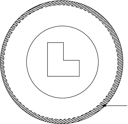
Figure 1. Illustration of the different domains in $\mathbb{R}^{2}$. The domain of interest $D$ is a L-shaped domain, $\Omega\subset\Omega^{M}(t)$ are interior of discs, and $B^{M}(t)$ is the filled portion of $\Omega^{M}(t)$.

Lemma 6.1 (Truncation error).

Let $\eta\in L^{2}(D)$, $e(t):=v(\tilde{\eta},t)-v^{M}(\tilde{\eta},t)$ and $c$ be the constant appearing in (55). There is a positive constant $C$ not depending on $M$ and t satisfying

(56) $$\|e(t)\|_{L^{2}(\Omega^{M}(t))}\leq Ce^{-\max(1,t)cM/t}\|\eta\|_{L^{2}(D)}.$$

Proof.

In this proof $C$ denotes a generic constant only depending on $\Omega$. Note that $e(t)$ satisfies the relations

(57) $$(e(t),\phi)+t^{2}d_{\Omega^{M}(t)}(e(t),\phi) =0,\quad\forall\phi\in H^{1}_{0}(\Omega^{M}(t)),$$

$$e(t) =v(t),\quad\hbox{on }\partial\Omega^{M}(t).$$

Let $\chi(t)\geq 0$ be a bounded cut off function satisfying $\chi(t)=1$ on $\partial\Omega^{M}(t)$ and $\chi(t)=0$ on $\Omega^{M}(t)\setminus B^{M}(t)$. Without loss of generality, we may assume that $\|\nabla\chi(t)\|_{L^{\infty}({{\mathbb{R}}^{d}})}\leq C/t$. This implies

$$\begin{split}\|\chi(t)v(t)\|_{L^{2}(B^{M}(t))}&+t\|\nabla(\chi(t)v(t))\|_{L^{2}(B^{M}(t))}\\ &\leq C(\|v(t)\|_{L^{2}(B^{M}(t))}+t\|\nabla v(t)\|_{L^{2}(B^{M}(t))})\\ &\leq Ce^{-\max(1,t)cM/t}\|\eta\|_{L^{2}(D)}.\end{split}$$

Here we use the decay estimate (55) for last inequality above. Now, setting $e(t):=\chi(t)v(t)+\zeta(t)$, we find that $\zeta(t)\in H^{1}_{0}(\Omega^{M}(t))$ satisfies

$$(\zeta(t),\phi)_{{\Omega^{M}(t)}}+t^{2}d_{\Omega^{M}(t)}(\zeta(t),\phi)=-(\chi(t)v(t),\phi)_{{\Omega^{M}(t)}}-t^{2}d_{\Omega^{M}(t)}(\chi(t)v(t),\phi)$$

for all $\phi\in H^{1}_{0}(\Omega^{M}(t))$. Taking $\phi=\zeta(t)$, we deduce that

$$\|\zeta(t)\|^{2}_{L^{2}(\Omega^{M}(t))}+t^{2}\|\nabla\zeta(t)\|^{2}_{L^{2}(\Omega^{M}(t))} \leq\|\chi(t)v(t)\|^{2}_{L^{2}(B^{M}(t))}+t^{2}\|\nabla(\chi(t)v(t))\|^{2}_{L^{2}(B^{M}(t))}$$

$$\leq Ce^{-2\max(1,t)cM/t}\|\eta\|^{2}_{L^{2}(D)}.$$

Thus, combining the estimates for $\zeta(t)$ and $\chi(t)v(t)$ completes the proof. ∎

Lemma 6.1 above is instrumental to derive exponentially decaying consistency error as $M\to\infty$. Indeed, we have the following theorem.

Theorem 6.2 (Truncation error).

Let $c$ be the constant appearing in (55) and assume $M>2(s+1)/c$. Then, there is a positive constant $C$ not depending on $M$ nor $k$ satisfying

(58) $$|a^{k}(\eta,\theta)-a^{k,M}(\eta,\theta)|\leq Ce^{-cM}\|\eta\|_{L^{2}(D)}\|\theta\|_{L^{2}(D)},\qquad\hbox{for all }\eta,\theta\in L^{2}(D).$$

Proof.

In this proof $C$ denotes a generic constant only depending on $\Omega$. Let $\eta,\theta$ be in $L^{2}(D)$. It suffices to bound

$$E :=\left|\frac{c_{s}k}{2}\sum_{j=-{N^{-}}}^{N^{+}}e^{sy_{j}}(w(t_{j})-w^{M}(t_{j}),\theta)_{D}\right|$$

$$\leq C\left(k\sum_{j=-{N^{-}}}^{-1}e^{sy_{j}}|(v(t_{j})-v^{M}(t_{j}),\theta)_{D}|+k\sum_{j=0}^{{N^{+}}}e^{sy_{j}}|(v(t_{j})-v^{M}(t_{j}),\theta)_{D}|\right)$$

$$=:E_{1}+E_{2}$$

with $v(t)=v(\widetilde{\eta},t)$ defined by (32) and $v^{M}(t)=v^{M}(\widetilde{\eta},t)$ defined by (54). We estimate $E_{1}$ and $E_{2}$ separately, starting with $E_{1}$.

From the definition $t_{j}=e^{-y_{j}/2}$, we deduce that when $j<0$, $t_{j}>1$ so that (56) gives

$$E_{1} \leq Cke^{-cM}\sum_{j=-{N^{-}}}^{-1}e^{sy_{j}}\|\eta\|_{L^{2}(D)}\|\theta\|_{L^{2}(D)}$$

$$\leq Ce^{-cM}\frac{ke^{-sk}}{1-e^{-sk}}\|\eta\|_{L^{2}(D)}\|\theta\|_{L^{2}(D)}\leq Ce^{-cM}\|\eta\|_{L^{2}(D)}\|\theta\|_{L^{2}(D)}.$$

Similarly, for $j\geq 0$, i.e. $t_{j}<1$, using (56) again, we have

$$E_{2} \leq Ck\sum_{j=0}^{{N^{+}}}e^{sy_{j}}e^{-{cM}/t_{j}}\|\eta\|_{L^{2}(D)}\|\theta\|_{L^{2}(D)}$$

$$\leq Ck\sum_{j=0}^{{N^{+}}}e^{sy_{j}}e^{-cM(1+y_{j}/2)}\|\eta\|_{L^{2}(D)}\|\theta\|_{L^{2}(D)}$$

$$=Cke^{-cM}\sum_{j=0}^{{N^{+}}}e^{(s-cM/2)y_{j}}\|\eta\|_{L^{2}(D)}\|\theta\|_{L^{2}(D)}$$

$$\leq Ce^{-cM}\frac{k}{1-\exp(k(s-cM/2))}\|\eta\|_{L^{2}(D)}\|\theta\|_{L^{2}(D)}$$

$$\leq\frac{Ce^{-cM}}{cM/2-s}\|\eta\|_{L^{2}(D)}\|\theta\|_{L^{2}(D)}\leq Ce^{-cM}\|\eta\|_{L^{2}(D)}\|\theta\|_{L^{2}(D)},$$

where we have also used the property $cM/2-s>1$ guaranteed by the assumption $M>2(s+1)/c$. ∎

6.3. Uniform Norm Equivalence on Convex Domains

Since the domains $\Omega^{M}(t)$ are convex, we know that the norms in $\dot{H}^{r}(\Omega^{M}(t))$ are equivalent to those in $H^{r}(\Omega)\cap H^{1}_{0}(\Omega^{M}(t))$ for $r\in[1,2]$, see e.g. [8]. However, as we mentioned in Remark 3.1, the equivalence constants depend a-priori on $\Omega^{M}(t)$ and therefore on $M$ and $t$. We show in this section that they can be bounded uniformly independently of both parameters.

To simplify the notation introduced in Section 3. We shall denote $T_{\Omega^{M}(t)}$ by $T_{t}$, $L_{{\Omega^{M}(t)}}$ by $L_{t}$ and $\dot{H}^{s}({\Omega^{M}(t)})$ by $\dot{H}^{s}$. We recall that $\Omega^{M}(t)$ is a dilatation of the convex and bounded domain $\Omega$ containing the origin, see (51). We then have the following lemma.

Lemma 6.3 (Ellipitic Regularity on Convex Domains).

Let $f\in L^{2}({\Omega^{M}(t)})$. Then $\theta:=T_{t}f$ is in $H^{2}(\Omega^{M}(t))\cap H^{1}_{0}(\Omega^{M}(t))$ and satisfies

(59) $$\|\theta\|_{H^{2}({\Omega^{M}(t)})}\leq C\|f\|_{L^{2}({\Omega^{M}(t)})},$$

where $C$ is a constant independent of $t$ and $M$.

Proof.

It is well known that the convexity of $\Omega$ and hence that of ${\Omega^{M}(t)}$ implies that the unique solution $\theta$ of (22) with $\omega$ replaced by ${\Omega^{M}(t)}$ is in $H^{2}(\Omega^{M}(t))\cap H^{1}_{0}(\Omega^{M}(t))$. Therefore, the crucial point is to show that the constant in (59) does not depend on $M$ or $t$. To see this, the $H^{2}$ elliptic regularity on convex domains implies that for $\hat{\theta}\in H^{1}_{0}(\Omega)$ with $\Delta\hat{\theta}\in L^{2}(\Omega)$ then $\hat{\theta}\in H^{2}(\Omega)$ and there is a constant $C$ only depending on $\Omega$ such that

(60) $$|\hat{\theta}|_{H^{2}(\Omega)}\leq C\|\Delta\hat{\theta}\|_{L^{2}(\Omega)}.$$

Here $|\cdot|_{H^{2}(\Omega)}$ denotes the $H^{2}(\Omega)$ seminorm. Let $\gamma$ be such that ${\Omega^{M}(t)}=\{\gamma x,\ x\in\Omega\}$ (see (51)) and $\hat{\theta}(\hat{x})=\theta(\gamma\hat{x})$ for $\hat{x}\in\Omega$. Once scaled back to $\Omega^{M}(t)$, estimate (60) gives

(61) $$|\theta|_{H^{2}({\Omega^{M}(t)})}\leq C\|\Delta\theta\|_{L^{2}({\Omega^{M}(t)})}=C\|f-\theta\|_{L^{2}({\Omega^{M}(t)})}.$$

Now (22) immediately implies that $\|\theta\|_{H^{1}({\Omega^{M}(t)}))}\leq\|f\|_{L^{2}({\Omega^{M}(t)})}$ and (59) follows by the triangle inequality and obvious manipulations. ∎

Remark 6.1 (Intermediate Spaces).

Lemma 6.3 implies that $D(L_{t})=\dot{H}^{2}=H^{2}({\Omega^{M}(t)})\cap H^{1}_{0}({\Omega^{M}(t)})$ with norm equivalence constants independent of $M$ and $t$. As $D(L_{t}^{1/2})=\dot{H}^{1}=H^{1}_{0}({\Omega^{M}(t)})$, for $s\in[1,2]$

$$\dot{H}^{s}=(H^{1}_{0}({\Omega^{M}(t)}),H^{2}({\Omega^{M}(t)})\cap H^{1}_{0}({\Omega^{M}(t)}))_{s-1,2}{=H^{s}({\Omega^{M}(t)})\cap H^{1}_{0}({\Omega^{M}(t)})}$$

with with norm equivalence constants independent of $M$ and $t$.

Lemma 6.4 (Norm Equivalence).

For $\beta\in[1,3/2)$, let $\theta$ be in $\dot{H}^{\beta}$ and $\widetilde{\theta}$ denote its extension by zero outside of ${\Omega^{M}(t)}$. Then $\widetilde{\theta}$ is in $H^{\beta}({{\mathbb{R}}^{d}})$ and

$$\|\theta\|_{\dot{H}^{\beta}}\leq C\|\widetilde{\theta}\|_{H^{\beta}({{\mathbb{R}}^{d}})}$$

with $C$ not depending on $t$ or $M$.

Proof.

Given $\theta\in H^{1}({\Omega^{M}(t)})$, we denote $R\theta$ to be the elliptic projection of $\theta$ into $H^{1}_{0}({\Omega^{M}(t)})$, i.e., $R\theta\in H^{1}_{0}({\Omega^{M}(t)})$ is the solution of

$$(R\theta,\phi)_{{\Omega^{M}(t)}} +d_{\Omega^{M}(t)}(R\theta,\phi)$$

$$=(\theta,\phi)_{{\Omega^{M}(t)}}+d_{\Omega^{M}(t)}(\theta,\phi),\qquad\hbox{for all }\phi\in H^{1}_{0}({\Omega^{M}(t)}).$$

It immediately follows that

$$\|R\theta\|_{\dot{H}^{1}}=\|R\theta\|_{H^{1}({\Omega^{M}(t)})}\leq\|\theta\|_{H^{1}({\Omega^{M}(t)})}.$$

Also, if $\theta\in H^{2}({\Omega^{M}(t)})$, Lemma 6.3 (see also Remark 6.1) implies

$$\|R\theta\|_{\dot{H}^{2}}\leq C\|R\theta\|_{H^{2}({\Omega^{M}(t)})}\leq C\|\theta\|_{H^{2}({\Omega^{M}(t)})}$$

with $C$ not depending on $t$ or $M$. Hence, it follows by interpolation that

(62) $$\|R\theta\|_{\dot{H}^{\beta}}\leq C_{\beta}\|\theta\|_{(H^{1}({\Omega^{M}(t)}),H^{2}({\Omega^{M}(t)}))_{\beta-1,2}}.$$

Now when $\theta\in\dot{H}^{\beta}\subset H^{1}(\Omega^{M}(t))$, $R\theta=\theta$ so that in view of (62), it remains to show that

$$\|\theta\|_{(H^{1}({\Omega^{M}(t)}),H^{2}({\Omega^{M}(t)}))_{\beta-1,2}}\leq C\|\tilde{\theta}\|_{H^{\beta}({{\mathbb{R}}^{d}})},$$

for a constant $C$ independent of $M$ and $t$. To see this, note that $\widetilde{\theta}$ is in $H^{1}({{\mathbb{R}}^{d}})$ and the extension of $\nabla\theta$ by zero is in $H^{\beta-1}({{\mathbb{R}}^{d}})$ for $\beta<3/2$. We refer to Theorem 1.4.4.4 of [28] for a proof when $d=1$ and the techniques used in Lemma 4.33 of [22] for the extension to the higher dimensional spaces. This implies that $\widetilde{\theta}$ belongs to $H^{\beta}({{\mathbb{R}}^{d}})$. Moreover, the restriction operator is simultaneously bounded from $H^{j}({{\mathbb{R}}^{d}})$ to $H^{j}({\Omega^{M}(t)})$ for $j=1,2$. Hence, by interpolation again, we have that

$$\|\theta\|_{(H^{1}({\Omega^{M}(t)}),H^{2}({\Omega^{M}(t)}))_{\beta-1,2}}\leq\|\widetilde{\theta}\|_{H^{\beta}({{\mathbb{R}}^{d}})}.$$

This completes the proof of the lemma. ∎

7. Finite Element Approximation

In this section, we turn our attention to the finite element approximation of each subproblems (54) in $a^{k,M}(\cdot,\cdot)$. Throughout this section, we omit when no confusion is possible the subscript $j$ in $t_{j}$, i.e. we consider a generic $t$ keeping in mind that the subsequent statements only hold for $t=t_{j}$ with $j=-N^{-},...,N^{+}$. We also make the additional unrestrictive assumption that $\Omega$ used to define $\Omega^{M}(t)$ (see (51)) is polygonal. In turn, so are all the dilated domains $\Omega^{M}(t)$.

7.1. Finite Element Approximation of $a^{k,M}(\cdot,\cdot)$

For any polygonal domain $\omega$, let $\{\mathcal{T}_{h}(\omega)\}_{h>0}$ be a sequence of conforming subdivisions of $\omega$ made of simplices of maximal size diameter $h\leq 1$. We use the notation $\mathcal{T}^{M}_{h}(t):=\mathcal{T}_{h}(\Omega^{M}(t))$ for $t=t_{j}$, $j=-N^{-},...,N^{+}$, given by (38). We assume that the subdivisions on $D$ are shape-regular and quasi-uniform. This means that there exist universal constants $\sigma,\rho>0$ such that

(63) $$\sup_{h>0}\max_{T\in\mathcal{T}_{h}(D)}\left(\frac{\text{diam}(T)}{r(T)}\right)\leq\sigma,$$

(64) $$\sup_{h>0}\left(\frac{\max_{T\in\mathcal{T}_{h}(D)}\text{diam}(T)}{\min_{T\in\mathcal{T}_{h}(D)}\text{diam}(T)}\right)\leq\rho,$$

where $\text{diam}(T)$ stands for the diameter of $T$ and $r(T)$ for the radius of the largest ball contained in $T$. We also assume that these conditions hold as well for $\mathcal{T}^{M}_{h}(t_{j})$ with constants $\sigma,\rho$ not depending on $j$. We finally require that all the subdivisions match on $D$, i.e.

(65) $$\mathcal{T}_{h}(D)\subset\mathcal{T}^{M}_{h}(t_{j})$$

for each $j$. We discuss in Section 8 how to generate subdivisions meeting these requirements.

Define $\mathbb{V}_{h}(\omega)\subset H^{1}_{0}(\omega)$ to be the space of continuous piecewise linear finite element functions associated with $\mathcal{T}_{h}(\omega)$ with $\omega=D$ or $\Omega^{M}(t)$. Also, we use the short notation $\mathbb{V}_{h}^{M}(t):=\mathbb{V}_{h}(\Omega^{M}(t))$.

We are now in position to define the fully discrete/implementable problem. For $\eta_{h}$ and $\theta_{h}$ in $\mathbb{V}_{h}{(D)}$, the finite element approximation of $a^{k,M}(\cdot,\cdot)$ given by (52) is

(66) $$a_{h}^{k,M}(\eta_{h},\theta_{h}):=\frac{c_{s}k}{2}\sum_{j=-{N^{-}}}^{N^{+}}e^{sy_{j}}(w_{h}^{M}(\widetilde{\eta}_{h},t_{j}),\theta_{h})_{{D}}$$

with

(67) $$w^{M}_{h}(\widetilde{\eta}_{h},t):=\widetilde{\eta}_{h}|_{\Omega^{M}(t)}+v^{M}_{h}(t)$$

and where $v^{M}_{h}(t)\in\mathbb{V}_{h}^{M}(t)$ solves

(68) $$(v^{M}_{h}(t),\phi_{h})_{\Omega^{M}(t)}+t^{2}d_{\Omega^{M}(t)}(v^{M}_{h}(t),\phi_{h})=-(\widetilde{\eta}_{h},\phi_{h})_{\Omega^{M}(t)},\quad\forall\phi_{h}\in\mathbb{V}^{M}_{h}(t).$$

Remark 7.1 (Assumption (65)).

Two critical properties follow from (65). On the one hand, our analysis below relies on the fact that the extension by zero $\widetilde{v}_{h}$ of $v_{h}\in\mathbb{V}_{h}{(D)}$ belongs to all $\mathbb{V}_{h}^{M}(t)$. This property greatly simplifies the computation of $(w_{h}^{M}(\widetilde{\eta}_{h},t_{j}),\theta_{h})_{{D}}$ in (66).

The finite element approximation of the problem (4) is to find $u_{h}\in\mathbb{V}_{h}{(D)}$ so that

(69) $$a^{k,M}_{h}(u_{h},\theta_{h})=(f,\theta_{h})_{{D}}\qquad\hbox{for all }\theta_{h}\in\mathbb{V}_{h}{(D)}.$$

Analogous to Lemma 4.2, we have the following representation using K-functional. The proof of the lemma is similar to that of Lemma 4.2 and is omitted.

Lemma 7.1 (K-functional formulation on the discrete space).

For $\eta_{h}\in\mathbb{V}_{h}{(D)}$, there holds

$$(w_{h}^{M}(\widetilde{\eta}_{h},t),\eta_{h})_{D}=(w_{h}^{M}(\widetilde{\eta}_{h},t),\widetilde{\eta}_{h})_{\Omega^{M}(t)}=\ K_{h}(\widetilde{\eta}_{h},t),$$

where

$$K_{h}(\widetilde{\eta}_{h},t):=\min_{\varphi_{h}\in\mathbb{V}_{h}^{M}(t)}\left(\|\widetilde{\eta}_{h}-\varphi_{h}\|_{L^{2}(\Omega^{M}(t))}^{2}+t^{2}d_{{\Omega^{M}(t)}}(\varphi_{h},\varphi_{h})\right).$$

We emphasize that for $v_{h}\in\mathbb{V}_{h}^{M}(t)$, its extension by zero $\tilde{\eta}_{h}$ belongs to $H^{1}({{\mathbb{R}}^{d}})$ and therefore

(70) $$K_{h}(\tilde{v}_{h},t)\geq K(\tilde{v}_{h},t).$$

This property is critical in the proof of next theorem, which ensures the $\mathbb{V}_{h}(D)$-ellipticity of the discrete bilinear for $a_{h}^{k,M}$. Before describing this next result, we recall that according to (49)

$$|a(\eta_{h},\theta_{h})-a^{k}(\eta_{h},\theta_{h})|\leq\gamma(k)\|\eta_{h}\|_{\widetilde{H}^{\delta}(D)}\|\theta_{h}\|_{{\widetilde{H}^{s}}(D)}$$

with $\delta$ between $s$ and $\min(2-s,3/2)$ (since $\mathbb{V}_{h}(D)\subset\widetilde{H}^{3/2-\epsilon}(D)$ for any $\epsilon>0$) and $\gamma(k)\sim Ce^{-2\pi\mathsf{d}/k}$. Also, we note that from the quasi-uniform (63) and shape-regular (64) assumptions, there exists a constant $c_{I}$ only depending on $\sigma$ and $\rho$ such that for $r^{-}\leq r^{+}<3/2$, there holds

(71) $$\|v_{h}\|_{\widetilde{H}^{r^{+}}(D)}\leq c_{I}h^{r^{-}-r^{+}}\|v_{h}\|_{\widetilde{H}^{r^{-}}(D)},\qquad\forall v_{h}\in\mathbb{V}_{h}^{M}(t).$$

Theorem 7.2 ($\mathbb{V}_{h}{(D)}$-ellipticity).

Let $\delta$ in Theorem 5.1 between $s$ and $\min(2-s,3/2)$, $k$ be the quadrature spacing and $c_{I}$ be the inverse constant in (71). We assume that the quadrature parameters $N^{-}$ and $N^{+}$ are chosen according to (48). Let $\gamma(k)$ be given by (50) and assume that $k$ is chosen sufficiently small so that

$$c_{I}\gamma(k)h^{s-\delta}<1.$$

Then, there is a constant $c$ independent of $h,k$ and $M$ such that

$$a_{h}^{k,M}(\eta_{h},\eta_{h})\geq c\|\eta_{h}\|_{{\widetilde{H}^{s}}(D)}^{2},\qquad\hbox{for all }\eta_{h}\in\mathbb{V}_{h}(D).$$

Proof.

Let $\eta_{h}\in\mathbb{V}_{h}^{M}(t)$ so that $\widetilde{\eta}_{h}\in H^{1}({{\mathbb{R}}^{d}})$. We use the equivalence relations provided by Lemmas 4.2 and 7.1 together with the monotonicity property (70) to write

$$a_{h}^{k,M}(\eta_{h},\eta_{h})=\frac{c_{s}k}{2}\sum_{j=-{N^{-}}}^{N^{+}}e^{sy_{j}}K_{h}(\widetilde{\eta}_{h},t_{j})\geq\frac{c_{s}k}{2}\sum_{j=-{N^{-}}}^{N^{+}}e^{sy_{j}}K(\widetilde{\eta}_{h},t_{j})=a^{k}(\eta_{h},\eta_{h}).$$

The quadrature consistency bound (49) supplemented by an inverse inequality (71) yields

$$a_{h}^{k,M}(\eta_{h},\eta_{h})\geq a(\eta_{h},\eta_{h})-\gamma(k)\|\eta_{h}\|_{\widetilde{H}^{\delta}(D)}\|\eta_{h}\|_{{\widetilde{H}^{s}}(D)}\geq a(\eta_{h},\eta_{h})-c_{I}\gamma{(k)}h^{s-\delta}\|\eta_{h}\|_{{\widetilde{H}^{s}}(D)}^{2}.$$

The desired result follows from assumption $c_{I}\gamma(k)h^{s-\delta}<1$ and the coercivity of $a(\cdot,\cdot)$, see (21). ∎

7.2. Approximations on $\Omega^{M}(t)$

The fully discrete scheme (69) requires approximations by the finite element methods on domains $\Omega^{M}(t)$. Standard finite element argumentations would lead to estimates with constants depending on $\Omega^{M}(t)$ and therefore $M$ and $t$. In this section, we exhibit results where this is not the case due to the particular definition (51) of $\Omega^{M}(t)$.

We can use interpolation to develop approximation results for functions in the intermediate spaces with constants independent of $M$ and $t$. The Scott-Zhang interpolation construction [43] gives rise to an approximation operator $\pi^{sz}_{h}:H^{1}_{0}({\Omega^{M}(t)})\rightarrow\mathbb{V}_{h}^{M}(t)$ satisfying

$$\|\eta-\pi^{sz}_{h}\eta\|_{H^{1}({\Omega^{M}(t)})}\leq C\|\eta\|_{H^{1}({\Omega^{M}(t)})},$$

for all $\eta\in H^{1}_{0}({\Omega^{M}(t)})=\dot{H}^{1}$ and

$$\|\eta-\pi^{sz}_{h}\eta\|_{H^{1}({\Omega^{M}(t)})}\leq Ch\|\eta\|_{H^{2}({\Omega^{M}(t)})},$$

for all $\eta\in H^{2}({\Omega^{M}(t)})\cap H^{1}_{0}({\Omega^{M}(t)})=\dot{H}^{2}$. The Scott-Zhang argument is local so the constants appearing above depend on the shape regularity of the triangulations but not on $t$ or $M$. Interpolating the above inequalities shows that for all $r\in[0,1]$

(72) $$\inf_{\chi\in{{\mathbb{V}}_{h}^{M}(t)}}\|\eta-\chi\|_{H^{1}({\Omega^{M}(t)})}\leq Ch^{r}\|\eta\|_{\dot{H}^{1+r}},\qquad\hbox{for all }\eta\in\dot{H}^{1+r}$$

with $C$ not depending on $t$ or $M$.

Let $T_{t,h}$ denote the finite element approximation to $T_{t}$ given by (23), i.e., for $F\in\dot{H}^{-1}$, $T_{t,h}F:=w_{h}$ with $w_{h}\in\mathbb{V}_{h}^{M}(t)$ being the unique solution of

$$(w_{h},\phi)_{\Omega^{M}(t)}+d_{\Omega^{M}(t)}(w_{h},\phi)=\langle F,\phi\rangle,\qquad\hbox{for all }\phi\in\mathbb{V}_{h}^{M}(t).$$

The approximation result (72) and standard finite element analysis techniques implies that for any $r\in[0,1]$,

(73) $$\|T_{t}F-T_{t,h}F\|_{L^{2}({\Omega^{M}(t)})}\leq Ch^{1+r}\|T_{t}F\|_{\dot{H}^{1+r}}\leq Ch^{1+r}\|F\|_{\dot{H}^{-1+r}},$$

where the last inequality follows from interpolation since $\|T_{t}F\|_{H^{1}({\Omega^{M}(t)})}\leq\|F\|_{H^{-1}({\Omega^{M}(t)})}$ and (59) hold.

For $f\in L^{2}(\Omega^{M}(t))$, we define the operator

(74) $$S_{t}f:=\eta\in H^{1}_{0}({\Omega^{M}(t)})$$

satisfying,

$$d_{\Omega^{M}(t)}(\eta,\phi)=(f,\phi)_{\Omega^{M}(t)},\qquad\hbox{for all }\phi\in H^{1}_{0}({\Omega^{M}(t)})$$

and let $S_{t,h}f\in\mathbb{V}_{h}^{M}(t)$ denote its finite element approximation; compare with $T_{t}$ and $T_{h,t}$. Although the Poincaré constant depends on the diameter of ${\Omega^{M}(t)}$, we still have the following lemma.

Lemma 7.3.

There is a constant $C$ independent of $h$, $t$, or $M$ satisfying

$$\|S_{t}f-S_{t,h}f\|_{L^{2}({\Omega^{M}(t)})}\leq Ch^{2}\|f\|_{L^{2}({\Omega^{M}(t)})}.$$

Proof.

For $f\in L^{2}({\Omega^{M}(t)})$, set $e_{h}:=(S_{t}-S_{t,h})f$. The elliptic regularity estimate (61) on convex domain and Cea’s Lemma imply

$$\begin{split}|e_{h}|_{H^{1}({\Omega^{M}(t)})}&=\inf_{\chi_{h}\in{{\mathbb{V}}_{h}^{M}(t)}}|S_{t}f-\chi_{h}|_{H^{1}({\Omega^{M}(t)})}\leq Ch|S_{t}f|_{H^{2}({\Omega^{M}(t)})}\\ &\leq Ch\|\Delta S_{t}f\|_{L^{2}({\Omega^{M}(t)})}=Ch\|f\|_{L^{2}({\Omega^{M}(t)})},\end{split}$$

where $C$ is a constant independent of $h$, $t$ and $M$. Galerkin orthogonality and the above estimate give

$$\|e_{h}\|_{L^{2}({\Omega^{M}(t)})}^{2} =d_{\Omega^{M}(t)}(e_{h},S_{t}e_{h})=d_{\Omega^{M}(t)}(e_{h},(S_{t}-S_{t,h})e_{h})$$

$$\leq|e_{h}|_{H^{1}({\Omega^{M}(t)})}|(S_{t}-S_{t,h})e_{h}|_{H^{1}({\Omega^{M}(t)})}$$

$$\leq Ch|e_{h}|_{H^{1}({\Omega^{M}(t)})}\|e_{h}\|_{L^{2}({\Omega^{M}(t)})}.$$

Combining the above two inequalities and obvious manipulations completes the proof of the lemma. ∎

We shall also need norm equivalency on discrete scales. Let $({{\mathbb{V}}_{h}^{M}(t)},\|\cdot\|_{L^{2}({\Omega^{M}(t)})})$ and $({{\mathbb{V}}_{h}^{M}(t)},\|\cdot\|_{H^{1}({\Omega^{M}(t)})})$ denote ${{\mathbb{V}}_{h}^{M}(t)}$ normed with the norms in $L^{2}({\Omega^{M}(t)})$ and $H^{1}({\Omega^{M}(t)})$, respectively. We define $\|\cdot\|_{\dot{H}^{r}_{h}(\Omega^{M}(t))}$, or simply $\|\cdot\|_{\dot{H}^{r}_{h}}$, to be the norm in the interpolation space

$$\big{(}{{\mathbb{V}}_{h}^{M}(t)},\|\cdot\|_{L^{2}({\Omega^{M}(t)})}),({{\mathbb{V}}_{h}^{M}(t)},\|\cdot\|_{H^{1}({\Omega^{M}(t)})})\big{)}_{r,2}.$$

For $r\in[0,1]$, as the natural injection is a bounded map (with bound 1) from ${{\mathbb{V}}_{h}^{M}(t)}$ into $L^{2}({\Omega^{M}(t)})$ and $H^{1}_{0}({\Omega^{M}(t)})$, respectively, $\|v_{h}\|_{\dot{H}^{r}}\leq\|v_{h}\|_{\dot{H}^{r}_{h}}$, for all $v_{h}\in{{\mathbb{V}}_{h}^{M}(t)}$. For the other direction, one needs a projector into ${{\mathbb{V}}_{h}^{M}(t)}$ which is simultaneously bounded on $L^{2}({\Omega^{M}(t)})$ and $H^{1}_{0}({\Omega^{M}(t)})$. In the case of a globally quasi uniform mesh, it was shown by Bramble and Xu [12] that the $L^{2}({\Omega^{M}(t)})$ projector $\pi_{h}$ satisfies this property. Their argument is local, utilizing the inverse inequality (71) and hence leads to constants depending on those appearing in (63) and (64) but not $t$, $h$, or $M$. Interpolating these results gives, for $r\in[0,1]$,

(75) $$c\|v_{h}\|_{\dot{H}^{r}_{h}}\leq\|v_{h}\|_{\dot{H}^{r}}\leq\|v_{h}\|_{\dot{H}^{r}_{h}},\qquad\hbox{for all }v_{h}\in{{\mathbb{V}}_{h}^{M}(t)},$$

where $c$ is a constant independent of $h$, $M$ and $t$. The spaces for negative $r$ are defined by duality and the stability of the $L^{2}(\Omega^{M}(t))$-projection $\pi_{h}$ yields

(76) $$c\|v_{h}\|_{\dot{H}^{-r}}\leq\|v_{h}\|_{\dot{H}^{-r}_{h}}\leq\|v_{h}\|_{\dot{H}^{-r}}.\qquad\hbox{for all }v_{h}\in{{\mathbb{V}}_{h}^{M}(t)}.$$

We finally note that a discrete version of Lemma 3.1 holds. Its proof is essentially the same and is omitted for brevity.

Lemma 7.4.

Let $a$ be in $[0,2]$ and $b$ be in $[0,1]$ with $a+b\leq 2$. Then for any $\mu\in(0,\infty)$,

$$\|(\mu I+T_{t,h})^{-1}\eta_{h}\|_{\dot{H}^{-b}_{h}}\leq\mu^{(a+b)/2-1}\|\eta_{h}\|_{\dot{H}^{a}_{h}},\qquad\hbox{for all }\eta_{h}\in{{\mathbb{V}}_{h}^{M}(t)}.$$

7.3. Consistency

The next step is to estimate the consistency error between $a^{k,M}(\cdot,\cdot)$ and $a_{h}^{k,M}(\cdot,\cdot)$ on $\mathbb{V}_{h}(D)$. Its decay depends on a parameter $\beta\in(s,3/2)$, which will be related later to the regularity of the solution $u$ to (4).

Theorem 7.5 (Finite Element Consistency).

Let $\beta\in(s,3/2)$. We assume that the quadrature parameters $N^{-}$ and $N^{+}$ are chosen according to (48). There exists a constant $C$ independent of $h$, $k$ and $M$ satisfying

(77) $$|a^{k,M}(\eta_{h},\theta_{h}) -a^{k,M}_{h}(\eta_{h},\theta_{h})|$$

$$\leq C(1+\ln(h^{-1}))h^{\beta-s}\|\eta_{h}\|_{\widetilde{H}^{\beta}(D)}\|\theta_{h}\|_{\widetilde{H}^{s}(D)}$$

for all $\eta_{h},\theta_{h}\in\mathbb{V}_{h}{(D)}$.

Proof.

In this proof, $C$ denotes a generic constant independent of $h$, $M$, $k$ and $t$.

Fix $\eta_{h}\in\mathbb{V}_{h}(D)$ and denote by $\tilde{\eta}_{h}$ its extension by zero outside $D$. We first observe that for $\theta_{h}\in\mathbb{V}_{h}(D)$ and $\tilde{\theta}_{h}$ its extension by zero outside $D$, we have

(78) $$(w^{M}(\widetilde{\eta}_{h},t_{j}),\theta_{h})_{D} =(\pi_{h}w^{M}(\widetilde{\eta}_{h},t_{j}),\widetilde{\theta}_{h})_{\Omega^{M}(t)},$$

where $\pi_{h}$ denotes the $L^{2}$ projection onto $\mathbb{V}_{h}(\Omega^{M}(t))$. Using the above identity and recalling that $t_{j}=e^{-y_{j}/2}$, we obtain

$$\begin{split}a^{k,M}(\eta_{h},\theta_{h})-a^{k,M}_{h}(\eta_{h},\theta_{h})=\frac{c_{s}}{2}\underbrace{k\sum_{t_{j}\leq\frac{1}{2}}e^{sy_{j}}(\pi_{h}w^{M}(\widetilde{\eta}_{h},t_{j})-w^{M}_{h}(\widetilde{\eta}_{h},t_{j}),\widetilde{\theta}_{h})_{\Omega^{M}(t)}}_{=:E_{1}}\\ +\frac{c_{s}}{2}\underbrace{k\sum_{t_{j}>\frac{1}{2}}e^{sy_{j}}(\pi_{h}w^{M}(\widetilde{\eta}_{h},t_{j})-w^{M}_{h}(\widetilde{\eta}_{h},t_{j}),\widetilde{\theta}_{h})_{\Omega^{M}(t)}}_{=:E_{2}}.\end{split}$$

We bound the two terms separately and start with the latter.

$\boxed{1}$ In view of the definitions (53) of $w^{M}(t)$ and (67) of $w^{M}_{h}(t)$, we have

(79) $$\pi_{h}w^{M}(\widetilde{\eta}_{h},t)-w^{M}_{h}(\widetilde{\eta}_{h},t)=\pi_{h}v^{M}(\widetilde{\eta}_{h},t)-v^{M}_{h}(\widetilde{\eta}_{h},t).$$

We recall that $T_{t}=T_{\Omega^{M}(t)}$ and $S_{t}$ are defined by (23) and (74) respectively. Using these operators and the relations satisfied by $v^{M}(t)$ and $v_{h}^{M}(t)$ (see (54) and (68)), we arrive at

(80) $$\pi_{h}w^{M}(\widetilde{\eta}_{h},t) -w^{M}_{h}(\widetilde{\eta}_{h},t)=[S_{t,h}(S_{t,h}+t^{2}I)^{-1}-\pi_{h}S_{t}(S_{t}+t^{2}I)^{-1}]\widetilde{\eta}_{h}$$

$$=t^{2}(S_{h,t}+t^{-2}I)^{-1}\pi_{h}(S_{t,h}-S_{t})(S_{t}+t^{2}I)^{-1}\widetilde{\eta}_{h}.$$

Thus,

$$\|\pi_{h}w^{M}(\widetilde{\eta}_{h},t) -w^{M}_{h}(\widetilde{\eta}_{h},t)\|_{L^{2}({\Omega^{M}(t)})}$$

$$\leq t^{2}\|(S_{t,h}+t^{2}I)^{-1}\pi_{h}(S_{t,h}-S_{t})(S_{t}+t^{2}I)^{-1}\|\ \|\widetilde{\eta}_{h}\|_{L^{2}({\Omega^{M}(t)})}$$

$$\leq t^{2}\|(S_{t,h}+t^{2}I)^{-1}\pi_{h}\|\ \|S_{t,h}-S_{t}\|\ \|(S_{t}+t^{2}I)^{-1}\|\ \|\widetilde{\eta}_{h}\|_{L^{2}({\Omega^{M}(t)})}.$$

Here we have used $\|\cdot\|$ to denote the operator norm of operators from $L^{2}({\Omega^{M}(t)})$ to $L^{2}({\Omega^{M}(t)})$. Combining

$$\|(S_{t,h}+t^{2}I)^{-1}\pi_{h}\|\leq t^{-2},\quad\|(S_{t}+t^{2}I)^{-1}\|\leq t^{-2}$$

and Lemma 7.3 gives

$$\|\pi_{h}w^{M}(\widetilde{\eta}_{h},t)-w^{M}_{h}(\widetilde{\eta}_{h},t)\|\leq Ct^{-2}h^{2}\|\widetilde{\eta}_{h}\|_{L^{2}({\Omega^{M}(t)})}.$$

Whence,

$$|E_{2}| \leq Ch^{2}k\sum_{t_{j}>\frac{1}{2}}e^{(s+1)jk}\|{\widetilde{\eta}_{h}}\|_{L^{2}({\Omega^{M}(t)})}\|{\widetilde{\theta}_{h}}\|_{L^{2}({\Omega^{M}(t)})}$$

$$\leq Ch^{2}\|\eta_{h}\|_{L^{2}(D)}\|\theta_{h}\|_{L^{2}(D)}\left(k\sum_{jk<2\ln 2}e^{(s+1)jk}\right)\leq Ch^{2}\|\eta_{h}\|_{L^{2}(D)}\|\theta_{h}\|_{L^{2}(D)}.$$

$\boxed{2}$ We now focus on $E_{1}$ which requires a finer analysis using intermediate spaces. Also, we argue differently for $\beta\in(1,3/2)$ and for $\beta\in(s,1]$. In either case, we define

$$\epsilon:=\min\{1-s,1/\ln(1/h)\}$$

and note that

(81) $$\epsilon^{-1}\leq c(1+\ln(1/h))\quad\hbox{and}\quad h^{-\epsilon}\leq c$$

with $c$ depending on $s$ but not $h$.

When $\beta\in(1,3/2)$, we invoke (79) again to deduce

(82) $$|E_{1}|\leq k\sum_{t_{j}\leq\frac{1}{2}}e^{sy_{j}}\|\pi_{h}v^{M}(\widetilde{\eta}_{h},t_{j})-v^{M}_{h}(\widetilde{\eta}_{h},t_{j})\|_{\dot{H}^{-s}_{h}}\|\widetilde{\theta}_{h}\|_{\dot{H}^{s}_{h}}.$$

We set $\mu(t):=t^{-2}-1$ and compute

(83) $$\pi_{h}v^{M}(\widetilde{\eta}_{h},t) -v^{M}_{h}(\widetilde{\eta}_{h},t)=t^{-2}[(I+\mu(t)T_{t,h})^{-1}T_{t,h}-\pi_{h}T_{t}(I+\mu(t)T_{t})^{-1}]\widetilde{\eta}_{h}$$

$$=(t\mu(t))^{-2}(\mu(t)^{-1}I+T_{t,h})^{-1}\pi_{h}(T_{t,h}-T_{t})(\mu(t)^{-1}I+T_{t})^{-1}\widetilde{\eta}_{h},$$

which is now estimated in three parts. Lemma 3.1 guarantees that

$$\|(\mu(t)^{-1}I+T_{t})^{-1}\|_{\dot{H}^{\beta}\rightarrow\dot{H}^{\beta-2}}\leq 1,$$

where we recall that $\dot{H}^{s}$ stands for $\dot{H}^{s}(\Omega^{M}(t))$. For the second part, the error estimate (73) with $1+r=\beta$ reads

$$\|T_{t,h}-T_{t}\|_{\dot{H}^{\beta-2}\rightarrow L^{2}(\Omega^{M}(t))}\leq Ch^{\beta}.$$

We estimate the last term of the product in the right hand side of (83) by

$$\|(\mu(t)^{-1} +T_{t,h})^{-1}\pi_{h}\|_{L^{2}(\Omega^{M}(t))\rightarrow\dot{H}^{-s}_{h}}$$

$$\leq C\|(\mu(t)^{-1}+T_{t,h})^{-1}\|_{\dot{H}^{s+\epsilon}_{h}\rightarrow\dot{H}^{-s}_{h}}\|\pi_{h}\|_{L^{2}(\Omega^{M}(t))\rightarrow\dot{H}^{s+\epsilon}_{h}}.$$

Thus, Lemma 7.4, the inverse estimate and (81) yield

$$\|(\mu(t)^{-1}+T_{t,h})^{-1}\pi_{h}\|_{L^{2}(\Omega^{M}(t))\rightarrow\dot{H}^{-s}_{h}}\leq Ch^{-s-\epsilon}t^{(2s+\epsilon-2)}\leq Ch^{-s}t^{(2s+\epsilon-2)}.$$

Note that for $t\in(0,1/2]$, $0<t^{2}\leq\mu(t)^{-1}\leq\frac{4}{3}t^{2}\leq\frac{1}{3}$ so that

$$(t\mu(t))^{-2}\leq\frac{16t^{2}}{9}.$$

Combining the above estimates with (83) gives

(84) $$\|\pi_{h}v^{M}(\widetilde{\eta}_{h},t)-v^{M}_{h}(\widetilde{\eta}_{h},t)\|_{\dot{H}^{-s}_{h}}\leq Ct^{2s+\epsilon}h^{\beta-s}\|\widetilde{\eta}_{h}\|_{\dot{H}^{\beta}},$$

Since $t_{j}=e^{-y_{j}/2}$,

$$e^{sy_{j}}t_{j}^{2s+\epsilon}=e^{-\epsilon y_{j}/2}.$$

Estimates (82), (84) and (75) then yield

(85) $$|E_{1}| \leq Ch^{\beta-s}k\sum_{ky_{j}\geq 2\ln 2}e^{-\epsilon y_{j}/2}\|\widetilde{\eta}_{h}\|_{\dot{H}^{\beta}}\|\widetilde{\theta}_{h}\|_{\dot{H}^{s}}$$

$$\leq Ch^{\beta-s}\epsilon^{-1}\|\widetilde{\eta}_{h}\|_{\dot{H}^{\beta}}\|\widetilde{\theta}_{h}\|_{\dot{H}^{s}}.$$

$$3$$ We bound the norms on $\Omega^{M}(t)$ by norms on $D$ using (25) with $r=s$ and Lemma 6.4 to arrive at

$$|E_{1}| \leq Ch^{\beta-s}\epsilon^{-1}\|\widetilde{\eta}_{h}\|_{H^{\beta}({{\mathbb{R}}^{d}})}\|\theta_{h}\|_{\dot{H}^{s}(D)}.$$

Applying the norm equivalence (24) gives

(86) $$|E_{1}|\leq Ch^{\beta-s}\epsilon^{-1}\|\eta_{h}\|_{\widetilde{H}^{\beta}(D)}\|\theta_{h}\|_{\widetilde{H}^{s}(D)}.$$

$$4$$ When $\beta\in(s,1]$, we bound (83) using different norms. In fact, we have

$$\|(\mu(t)^{-1}I+T_{t})^{-1}\|_{\dot{H}^{\beta}\rightarrow\dot{H}^{-1}}\leq t^{\beta-1},\quad\|T_{t,h}-T_{t}\|_{\dot{H}^{-1}\rightarrow L^{2}(\Omega^{M}(t))}\leq Ch,$$

and by Lemma 7.4,

$$\|(\mu(t)^{-1}+T_{t,h})^{-1} \pi_{h}\|_{L^{2}(\Omega^{M}(t))\rightarrow\dot{H}^{-s}_{h}}$$

$$\leq\|(\mu(t)^{-1}+T_{t,h})^{-1}\pi_{h}\|_{\dot{H}^{1-\beta+s+\epsilon}\rightarrow\dot{H}^{-s}_{h}}\|\pi_{h}\|_{L^{2}({\Omega^{M}(t)})\rightarrow\dot{H}^{1-\beta+s+\epsilon}}$$

$$\leq Ch^{-1+\beta-s}t^{(2s+\epsilon-\beta-1)}.$$

These estimates lead (84) and hence (85) as well when $\beta\in(s,1]$. The remainder of the proof is the same as in the case $\beta\in(1,3/2)$ except that the norm equivalence (24) is invoked in place of Lemma 6.4.

$$5$$ The proof of the theorem is complete upon combining the estimates for $E_{1}$ and $E_{2}$. ∎

7.4. Error Estimates

Now that the consistency error between $a(\cdot,\cdot)$ and $a_{h}^{k,M}(\cdot,\cdot)$ is obtained, we can apply Strang’s lemma to deduce the convergence of the approximation $u_{h}$ towards $u$ in the energy norm. To achieve this, we need a result regarding the stability and approximability of the Scott-Zhang interpolant $\pi^{sz}_{h}$ [43] in the fractional spaces $\widetilde{H}^{\beta}(D)$.

This is the subject of the next lemma. Its proof is somewhat technical and given in Appendix A.

Lemma 7.6 (Scott-Zhang Interpolant).

Let $\beta\in(1,3/2)$. Then, there is a constant $C$ independent of $h$ such that

(87) $$\|\pi^{sz}_{h}v\|_{\widetilde{H}^{\beta}(D)}\leq C\|v\|_{\widetilde{H}^{\beta}(D)}$$

and for $s\in[0,1]$,

(88) $$\|\pi^{sz}_{h}v-v\|_{\widetilde{H}^{s}(D)}\leq Ch^{\beta-s}\|v\|_{\widetilde{H}^{\beta}(D)},$$

for all $v\in\widetilde{H}^{\beta}(D)$.

We note that the above lemma holds for $\beta\in(0,1)$ and $s\in(0,\beta)$ provided that $\pi^{sz}_{h}$ is replaced by $\pi_{h}$, the $L^{2}$ projection onto $\mathbb{V}_{h}(D)$; see e.g. Lemma 5.1 of [9]. In order to consider both case simultaneously in the following proof, we set $\Pi_{h}=\pi_{h}$ when $\beta\in[0,1]$ and $\Pi_{h}=\pi^{sz}_{h}$ when $\beta\in(1,3/2)$.

Theorem 7.7.

Assume that the solution $u$ of (5) belongs to $\widetilde{H}^{\beta}(D)$ for $\beta\in(s,3/2)$. Let $\delta:=\min(2-s,\beta)$ be as in Theorem 5.1, $k$ be the quadrature spacing and $c_{I}$ be the inverse constant in (71). We assume that the quadrature parameters $N^{-}$ and $N^{+}$ are chosen according to (48). Let $\gamma(k)$ be given by (50) and assume that $k$ is chosen sufficiently small so that

$$c_{I}\gamma(k)h^{s-\delta}<1.$$

Moreover, let $u_{h}\in\mathbb{V}_{h}(D)$ be the solution of (69). Then there is a constant $C$ independent of $h$, $M$ and $k$ satisfying

(89) $$\|u-u_{h}\|_{\widetilde{H}^{s}(D)}\leq C(\gamma(k)+e^{-cM}+(1+\ln{(h^{-1})})h^{\beta-s})\|u\|_{\widetilde{H}^{\beta}(D)}.$$

Proof.

In our context, the first Strang lemma (see e.g. Theorem 4.1.1 in [15]) reads

$$\|u-u_{h}\|_{{\widetilde{H}^{s}}(D)}\leq C\inf_{v_{h}\in\mathbb{V}_{h}{(D)}}\left(\|u-v_{h}\|_{{\widetilde{H}^{s}}(D)}+\sup_{w_{h}\in\mathbb{V}_{h}{(D)}}\frac{|(a-a_{h}^{k,M})(v_{h},w_{h})|}{\|w_{h}\|_{{\widetilde{H}^{s}}(D)}}\right),$$

where $C$ is a constant independent of $h$, $k$ and $M$. From the consistency estimates (49), (58) and (77), we deduce that

$$\|u-u_{h}\|_{\widetilde{H}^{s}(D)} \leq C\|u-\Pi_{h}u\|_{\widetilde{H}^{s}(D)}$$

$$\qquad+C(\gamma(k)+e^{-cM}+(1+\ln{(h^{-1})})h^{\beta-s})\|\Pi_{h}u\|_{\widetilde{H}^{\beta}(D)}$$

The desired estimate follows from the approximability and stability of $\Pi_{h}$. ∎

8. Numerical implementation and results

In this section, we present detailed numerical implementation to solve the following model problems.

8.1. Model Problems.

One of the difficulties in developing numerical approximation to (5) is that there are relatively few examples where analytical solutions are available. One exception is the case when $D$ is the unit ball in ${{\mathbb{R}}^{d}}$. In that case, the solution to the variational problem

(90) $$a(u,\phi)=(1,\phi)_{D},\qquad\hbox{for all }\phi\in{\widetilde{H}^{s}}(D)$$

is radial and given by, (see [21])

(91) $$u(x)=\frac{2^{-2s}\Gamma(d/2)}{\Gamma(d/2+s)\Gamma(1+s)}(1-|x|^{2})^{s}$$

It is also possible to compute the right hand side corresponding to the solution $u(x)=1-|x|^{2}$ in the unit ball. The corresponding right hand side can be derived by first computing the Fourier transform of $\widetilde{u}$, i.e.,

$${\mathcal{F}}(\widetilde{u})=2J_{2}(|\zeta|)/|\zeta|^{2},$$

where $J_{n}$ is the Bessel function of the first kind. When $0<s<1$, we obtain

(92) $$f(x)={\mathcal{F}}^{-1}(2|\zeta|^{2s-2}J_{2}(|\zeta|))=\frac{2^{2s}\Gamma(d/2+s)}{\Gamma(d/2)\Gamma(2-s)}{}_{2}F_{1}\left(d/2+s,s-1,d/2,|x|^{2}\right),$$

where ${}_{2}F_{1}$ is the Gaussian or ordinary hypergeometric function.

Remark 8.1 (Smoothness).

Even though the solution $u(x)=1-|x|^{2}$ is infinitely differentiable on the unit ball, the right hand side $f$ has limited smoothness. Note that $f$ is the restriction of $(-\Delta)^{s}\widetilde{u}$ to the unit ball. Now $\widetilde{u}\in H^{3/2-\epsilon}({{\mathbb{R}}^{d}})$ for $\epsilon>0$ but is not in $H^{3/2}({{\mathbb{R}}^{d}})$. This means that $(-\Delta)^{s}\widetilde{u}$ is only in $H^{3/2-2s-\epsilon}({{\mathbb{R}}^{d}})$ and hence $f$ is only in $H^{3/2-2s-\epsilon}(\Omega)$. This is in agreement with the singular behavior of ${}_{2}F_{1}\left(d/2+s,s-1,d/2,t\right)$ at $t=1$ (see [39], Section 15.4). In fact,

$${}_{2}F_{1}\left(d/2+s,s-1,d/2,1\right) =\frac{\Gamma(d/2+s)\Gamma(1-2s)}{\Gamma(d/2+1-s)\Gamma(-s)}\quad\hbox{when }0<s<1/2,$$

$$\lim_{t\rightarrow 1^{-}}\frac{{}_{2}F_{1}\left(d/2+s,s-1,d/2,t\right)}{-\log(1-t)} =\frac{\Gamma(d/2)}{\Gamma(-1/2)\Gamma(1/2)}\quad\hbox{when }s=1/2,$$

$$\lim_{t\rightarrow 1^{-}}\frac{{}_{2}F_{1}\left(d/2+s,s-1,d/2,t\right)}{(1-t)^{-2s+1}} =\frac{\Gamma(d/2)}{\Gamma(-1/2)\Gamma(1/2)}\quad\hbox{when }1/2<s<1.$$

This implies that for $s\geq 1/2$, the trace on $|x|=1$ of $f(x)$ given by (92) fails to exist (as for generic functions in $H^{3/2-2s}({{\mathbb{R}}^{d}})$). This singular behavior affects the convergence rate of the finite element method when the finite element data vector is approximated using standard numerical quadrature (e.g. Gaussian quadrature).

8.2. Numerical Implementation

Based on the notations in Section 6, we set $\Omega=D$ to be either the unit disk in ${\mathbb{R}}^{2}$ or $D=(-1,1)$ in ${\mathbb{R}}$. Let $\Omega^{M}(t)$ be corresponding dilated domains. In one dimensional case, we consider $\mathcal{T}_{h}(D)$ to be a uniform mesh and $\mathbb{V}_{h}(D)$ to be the continuous piecewise linear finite element space. For the two dimensional case, $\mathcal{T}_{h}(D)$ a regular (in the sense of page 247 in [15]) subdivision made of quadrilaterals. In this case, $\mathbb{V}_{h}(D)$ is the set of continuous piecewise bilinear functions.

Non-uniform Meshes for ${\Omega^{M}(t)}$

We extend $\mathcal{T}_{h}(D)$ to non-uniform meshes $\mathcal{T}^{M}_{h}(t)$, thereby violating the quasi-uniform assumption. For $t\leq 1$, we use a quasi-uniform mesh on $\Omega^{M}(t)=\Omega^{M}(1)$ with the same mesh size $h$. When $t>1$ and $D=(-1,1)$, we use an exponentially graded mesh outside of $D$, i.e. the mesh points are $\pm e^{ih_{0}}$ for $i=1,\ldots,\lceil M/h\rceil$ with $h_{0}=h(\ln{\gamma})/M$, where $\gamma$ is the radius of ${\Omega^{M}(t)}$ (see (51)). Therefore, we maintain the same number of mesh points for all $\Omega^{M}(t)$. When $D$ is a unit disk in ${\mathbb{R}}^{2}$, we start with a coarse subdivision of ${\Omega^{M}(t)}$ as in the left of Figure 2 (the coarse mesh of $D$ in grey). Note that all vertices of a square have the same radial coordinates. We also point out that the position of the vertices along the radial direction and outside of $D$ follow the same exponential distribution as in the one dimensional case. Then we refine each cell in $D$ by connecting the midpoints between opposite edges. For the cells outside of $D$, we consider the same refinement in the polar coordinate system $(\ln r,\theta)$ with $r>1$ and $\theta\in[0,2\pi]$. This guarantees that mesh points on the same radial direction still follows the exponential distribution after global refinements and the number of mesh points in $\mathcal{T}^{M}_{h}(t)$ is unchanged for all $t>0$. The figure on the right of Figure 2 shows the exponentially graded mesh after three times global refinement.

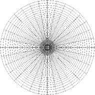
Figure 2. Coarse gird (left) and three-times-refined non-uniform grid (right) of $\Omega^{M}(t)$ with $M=4$ and $t=1$. Grids of $D$ are in grey.

Matrix Aspects

To express the linear system to be solved, we denote by $U$ to be the coefficient vector of $u_{h}$ and $F$ to be the coefficient vector of the $L^{2}$ projection of $f$ onto $\mathbb{V}_{h}(D)$. Let $M_{h}(t)$ and $A_{h}(t)$ be the mass and stiffness matrix in $\mathbb{V}^{M}_{h}(t)$. Denote $M_{D,h}$ to be the mass matrix in $\mathbb{V}_{h}(D)$. The linear system is given by

(93) $$\frac{\sin{(\pi\beta)k}}{\pi}\sum_{i=-{N^{-}}}^{{N^{+}}}e^{sy_{i}}M_{D,h}(e^{y_{i}}M_{h}(t_{i})+A_{h}(t_{i}))^{-1}A_{h}(t_{i})U=F$$

with $y_{i}=ik$ and $t_{i}=e^{-y_{i}/2}$. Here ${M_{D,h}},\ U$ and $F$ are all extended by zeros so that the dimension of the system is equal to the dimension of $\mathbb{V}^{M}_{h}(t)$.

Preconditioner

Since the linear system is symmetric, we apply the Conjugate Gradient method to solve the above linear system. Due to the norm equivalence between $(L^{2}(D),H^{1}_{0}(D))_{s,2}$ and $\widetilde{H}^{s}(D)$, the condition number of the system matrix is bounded by $Ch^{-2s}$. In order to reduce the number of iterations in one dimensional space, we use fractional powers of the discrete Laplacian $L_{D,h}$ as a preconditioner, where $L_{D,h}:H^{1}_{0}(\Omega)\to L^{2}(D)$ is defined by

$$d_{D}(L_{D,h}w,\phi_{h})=d_{D}(w,\phi_{h}),\qquad\hbox{for all }\phi_{h}\in\mathbb{V}_{h}(D).$$

This can be computed by the discrete sine transform similar to the implementation discussed in [7]. More precisely, the matrix representation of $L_{D,h}$ is given by ${(M_{D,h})}^{-1}{A_{D,h}}$, where $A_{D,h}$ is stiffness matrix in $\mathbb{V}_{h}(D)$. The eigenvalues of $A_{D,h}$ and $M_{D,h}$ (for the same eigenvectors) are $a_{j}:=(2+\cos(j\pi h))/h$ and $m_{j}:=h(4+2\cos(j\pi h))/6$ for $j=1,\ldots,\dim(\mathbb{V}_{h}(D))$, respectively. Therefore, the eigenvalues of $L_{h}$ are given by $\lambda_{j,h}:=a_{j}/m_{j}$. We use

$$B:=S\Lambda S$$

as a preconditioner, where $S_{ij}:=\sqrt{2h}\sin({ij\pi h})$ and $\Lambda$ is the diagonal matrix whose diagonal entries are $\lambda_{j,h}^{-s}/m_{j}$. We also note that $S^{-1}=S$.

In two dimensional space, we use the multilevel preconditioner advocated in [11].

8.3. Numerical Illustration for the Non-smooth Solution

We first consider the numerical experiments for the model problem (90) and study the behavior of the $L^{2}(D)$ error.

Influence from the Sinc Quadrature and Domain Truncation.

When $D=(-1,1)$, we approximate the solution on the fixed uniform mesh with the mesh size $h=1/8192$. The domain truncation parameter $M$ is also fixed to be $20$. Thus, $h$ is small enough and $M$ is large enough so that the $L^{2}(D)$-error is dominant by the sinc quadrature spacing $k$. The left part of Figure 3 shows that the $L^{2}(D)$-error quickly converges to the error dominant by the Galerkin approximation when $k$ approaches zero. Similar results are observed from the right part of Figure 3 when the domain truncation parameter $M$ increases. In this case, the mesh size $h=1/8192$ and the quadrature step size $k=0.2$.

Error Convergence from the Finite Element Approximation

We note that we implement the numerical algorithm for the two dimensional case using the deal.ii Library [4] and we invert matrices in (93) using the direct solver from UMFPACK [20]. Figure 4 shows the approximated solutions for $s=0.3$ and $s=0.7$, respectively. Table 1 reports errors $\|u-u_{h}\|_{L^{2}(D)}$ and rates of convergence with $s=0.3,0.5$ and $0.7$. Here the quadrature spacing ($k=0.25$) and the domain truncation parameter ($M=4$) are fixed so that the finite element discretization dominates the error.

We note that Theorem 7.1 together with Theorem 5.4 in [29] (see also Proposition 2.7 in [10]) guarantees that when $\partial D$ is of class $C^{\infty}$ and $f$ is in $L^{2}(D)$, the solution of (5) is in $\widetilde{H}^{s+\alpha^{-}}(D)$ where

(94) $$\alpha:=\min\{s,1/2\}$$

and $\alpha^{-}$ denotes any number strictly smaller that $\alpha$. This indicates that the expected rate of convergence in $L^{2}(D)$ norm should be $\beta+\alpha^{-}-s$ if the solution $u$ is in $\widetilde{H}^{\beta}(D)$. Since the solution $u$ is in $H^{s+1/2-\epsilon}(D)$ (see [1] for a proof), Table 1 matches the expected rate of convergence $\min(1,s+1/2)$.

Figure 3. The above figures report the $L^{2}(D)$-error behavior when $D=(-1,1)$. The left one shows the error as a function of the quadrature spacing $k$ for a fixed mesh size ($h=1/8192$) and domain truncation parameter ($M=20$). The right plot reports the error as a function of the domain truncation parameter $M$ with fixed mesh size ($h=1/8192$) and quadrature spacing $(k=0.2)$. The spatial error dominates when $k$ is small (left) and $M$ is large (right).

$\#$DOFS	$s=0.3$		$s=0.5$		$s=0.7$
345	$2.69\times 10^{-1}$	-	$1.63\times 10^{-1}$	-	$1.03\times 10^{-1}$	-
1361	$1.59\times 10^{-1}$	0.7575	$9.07\times 10^{-2}$	0.8426	$5.55\times 10^{-2}$	0.8918
5409	$9.56\times 10^{-2}$	0.7323	$5.05\times 10^{-2}$	0.8438	$2.95\times 10^{-2}$	0.9091
21569	$5.71\times 10^{-2}$	0.7447	$2.78\times 10^{-2}$	0.8633	$1.54\times 10^{-2}$	0.9366
86145	$3.38\times 10^{-2}$	0.7547	$1.51\times 10^{-2}$	0.8832	$7.91\times 10^{-3}$	0.9641
344321	$1.99\times 10^{-2}$	0.7644	$8.07\times 10^{-3}$	0.9004	$3.97\times 10^{-3}$	0.9936

Table 1. $L^{2}(D)$-errors for different values of $s$ versus the number of degree of freedom used for the 2-D nonsmooth computations. $\#$DOFS denotes the dimension of the finite element space ${{\mathbb{V}}_{h}^{M}(t)}.$

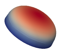
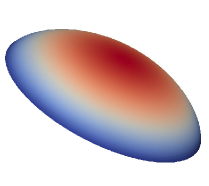
Figure 4. Approximated solutions of (91) for $s=0.3$ (left) and $s=0.7$ (right) on the unit disk.

8.4. Numerical Illustration for the Smooth Solution

When the solution is smooth, the finite element error (assuming the exact computation of the stiffness entries, i.e. no consistency error) satisfies

$$\|u-u_{h}\|_{L^{2}(D)}\leq ch^{2-s+\alpha^{-}},$$

where $\alpha$ is given by (94). In contrast, because of the inherent consistency error, our method only guarantees (c.f., Theorem 7.7)

(95) $$\|u-u_{h}\|_{L^{2}(D)}\leq ch^{3/2-s+\alpha^{-}}.$$

Table 2 reports $L^{2}(D)$-errors and rates for the problem (5) with the smooth solution $u(x)=1-|x|^{2}$ and the corresponding right hand side data (92) in the unit disk. To see the error decay, here we choose the quadrature step size $k=0.2$ and the domain truncation parameter $M=5$. The observed decay in the error does not match the expected rate (95). We think this loss of accuracy may be due either to the deterioration of the shape regularity constant in generating the subdivisions of $\Omega^{M}(t)$ (see Section 8.2) or to the imprecise numerical integration of the singular right hand side in (92).

To illustrate this, we consider the one dimensional problem. Instead of using (92) to compute the right hand side vector, similar to (7), we compute

(96) $$(f,\phi_{j})=a(u,\phi_{j})=\frac{(\partial_{L}^{2s-1}\phi_{j},u^{\prime})_{D}+(\partial_{L}^{2s-1}u,\phi_{j}^{\prime})_{D}}{2\,\cos(s\pi)}$$

with $D=(-1,1)$. We note that when $s<1/2$, the fractional derivative with the negative power $2s-1$ still makes sense for the local basis function $\phi_{j}$. The right hand side of (96) can now be computed exactly.

$\#$DOFS	$s=0.3$		$s=0.5$		$s=0.7$
409	$6.24\times 10^{-2}$	-	$9.55\times 10^{-2}$	-	$1.35\times 10^{-1}$	-
1617	$2.90\times 10^{-2}$	1.10	$4.33\times 10^{-2}$	1.14	$6.27\times 10^{-2}$	1.10
6433	$1.44\times 10^{-2}$	1.01	$1.94\times 10^{-2}$	1.15	$2.81\times 10^{-2}$	1.16
25665	$7.21\times 10^{-3}$	1.00	$8.55\times 10^{-3}$	1.19	$1.20\times 10^{-2}$	1.23
102529	$3.56\times 10^{-3}$	1.02	$3.67\times 10^{-3}$	1.22	$4.78\times 10^{-3}$	1.32
409857	$1.74\times 10^{-3}$	1.04	$1.54\times 10^{-3}$	1.25	$1.73\times 10^{-3}$	1.47

Table 2. $L^{2}(D)$-errors and rates for $s=0.3$, $0.5$ and $0.7$ for the problem (5) with the right hand side (92). $\#$DOFS denotes the number of degree of freedoms of ${\Omega^{M}(t)}$.

We illustrate the convergence rate for the one dimensional case in Table 3 when the $L^{2}(D)$-projection of right hand side is computed from (96). In this case, we compute at $s=0.3,0.4,0.7$ as the expression in (96) is not valid for $s=0.5$. We also fix $k=0.2$ and $M=6$. In all cases, we observe the predicted rate of convergence $\min(3/2,2-s)$, see (95).

$h$	$s=0.3$		$s=0.4$		$s=0.7$
1/16	$4.51\times 10^{-4}$		$3.47\times 10^{-4}$		$9.27\times 10^{-4}$
1/32	$1.42\times 10^{-4}$	1.58	$1.02\times 10^{-4}$	1.77	$4.16\times 10^{-4}$	1.16
1/64	$4.25\times 10^{-5}$	1.63	$3.31\times 10^{-5}$	1.62	$1.80\times 10^{-4}$	1.21
1/128	$1.34\times 10^{-5}$	1.66	$1.14\times 10^{-5}$	1.54	$7.66\times 10^{-5}$	1.23
1/256	$4.43\times 10^{-6}$	1.59	$4.06\times 10^{-6}$	1.49	$3.21\times 10^{-5}$	1.25
1/512	$1.50\times 10^{-6}$	1.56	$1.46\times 10^{-6}$	1.48	$1.33\times 10^{-5}$	1.27

Table 3. $L^{2}(D)$-errors and rates for $s=0.3$, $0.4$ and $0.7$ for the one dimensional problem when right hand side of the discrete problem is computed by (96).

Appendix A Proof of Lemma 7.6

The proof of Lemma 7.6 requires the following auxiliary localization result. We refer to [26] for a similar result in two dimensional space.

Lemma A.1.

For $r\in(0,1/2)$, let $v$ be in $H^{r}(D)$ and $\widetilde{v}$ denote the extension by zero of $u$ to ${{\mathbb{R}}^{d}}$. There exists a constant $C$ independent of $h$ such that

$$\|\widetilde{v}\|_{H^{r}({{\mathbb{R}}^{d}})}^{2}\leq C\bigg{(}h^{-2r}\|v\|_{L^{2}(D)}^{2}+\sum_{\tau\in{\mathcal{T}_{h}(D)}}|v|_{H^{r}(\tau)}^{2}\bigg{)}$$

with a constant $C$ independent of $h$.

Proof.

Let $\widetilde{\mathcal{T}}_{h}(D)$ be any quasi-uniform mesh (satisfying (63) and (64)) which extends ${\mathcal{T}_{h}(D)}$ beyond a unit size neighborhood of $D$. Fix $\delta>0$ and for $\tau\in{\mathcal{T}_{h}(D)}$ set

$${\widetilde{\tau}}=\cup_{\{\eta\in\widetilde{\mathcal{T}}_{h}(D)\ :\ \hbox{dist}(\eta,\tau)<\delta h\}}\eta.$$

Let

$$D_{h}^{\delta}=\mathop{\bigcup}_{\tau\in{\mathcal{T}_{h}(D)}}{\widetilde{\tau}}$$

and let $\widetilde{\mathcal{T}}_{h}(D^{\delta}_{h})$ denote the set of $\tau\in\widetilde{\mathcal{T}}_{h}(D)$ contained in $D_{h}^{\delta}$. Finally, for $\tau\in\widetilde{\mathcal{T}}_{h}(D^{\delta}_{h})\setminus{\mathcal{T}_{h}(D)}$, set

$${\widetilde{\tau}}=\bigcup_{\{\eta\in\widetilde{\mathcal{T}}_{h}(D^{\delta}_{h})\ :\ \hbox{dist}(\eta,\tau)<\delta h\}}\eta.$$

Fix $v\in H^{r}(D)$. Since $\widetilde{v}$ vanishes outside of $D_{h}^{\delta}$,

$$|\widetilde{v}|_{H^{r}({{\mathbb{R}}^{d}})}^{2} =\int_{D_{h}^{\delta}}\int_{D_{h}^{\delta}}\frac{(\widetilde{v}(x)-\widetilde{v}(y))^{2}}{|x-y|^{d+2r}}\,dx\,dy$$

$$\qquad+2\int_{D}\int_{(D_{h}^{\delta})^{c}}\frac{v(y)^{2}}{|x-y|^{d+2r}}\,dx\,dy=:J_{1}+J_{2}.$$

The second integral above is bounded by

(97) $$J_{2} \leq 2\int_{D}\int_{|x-y|\geq\delta h}\frac{v(y)^{2}}{|x-y|^{d+2r}}\,dx\,dy$$

$$=2(\delta h)^{-2r}\int_{D}v(y)^{2}\,dy\int_{|z|\geq 1}|z|^{-d-2r}\,dz=Ch^{-2r}\|v\|_{L^{2}(D)}^{2}.$$

Expanding the first integral gives

(98) $$J_{1} =\sum_{\tau\in\widetilde{\mathcal{T}}_{h}(D^{\delta}_{h})}\int_{\tau}\int_{\widetilde{\tau}}\frac{(v(x)-v(y))^{2}}{|x-y|^{d+2r}}\,dx\,dy$$

$$\qquad+\sum_{\tau\in\widetilde{\mathcal{T}}_{h}(D^{\delta}_{h})}\int_{\tau}\int_{{\widetilde{\tau}}^{c}}\frac{(v(x)-v(y))^{2}}{|x-y|^{d+2r}}\,dx\,dy=:J_{3}+J_{4}.$$

Applying the arithmetic-geometric mean inequality gives

(99) $$J_{4}\leq 2\sum_{\tau\in\widetilde{\mathcal{T}}_{h}(D^{\delta}_{h})}\int_{\tau}\int_{{\widetilde{\tau}}^{c}}\frac{v(x)^{2}+v(y)^{2}}{|x-y|^{d+2r}}\,dx\,dy.$$

As in (97),

(100) $$J_{5}:=\sum_{\tau\in\widetilde{\mathcal{T}}_{h}(D^{\delta}_{h})}\int_{\tau}\int_{{\widetilde{\tau}}^{c}}\frac{v(y)^{2}}{|x-y|^{d+2r}}\ \,dx\,dy\leq Ch^{-2r}\|v\|_{L^{2}(D)}^{2}.$$

Now,

$$\{(\tau,\tau_{1}) \ :\ \tau\in\widetilde{\mathcal{T}}_{h}(D^{\delta}_{h})\hbox{ and }\tau_{1}\in{\widetilde{\tau}}^{c}\}$$

$$=\{(\tau,\tau_{1})\in\widetilde{\mathcal{T}}_{h}(D^{\delta}_{h})\times\widetilde{\mathcal{T}}_{h}(D^{\delta}_{h})\ :\ \hbox{dist}(\tau,\tau_{1})>\delta h\}$$

$$=\{(\tau,\tau_{1})\ :\ \tau_{1}\in\widetilde{\mathcal{T}}_{h}(D^{\delta}_{h})\hbox{ and }\tau\in{\widetilde{\tau}}_{1}^{c}\}.$$

Using this and Fubini’s Theorem gives

$$\sum_{\tau\in\widetilde{\mathcal{T}}_{h}(D^{\delta}_{h})} \int_{\tau}\int_{{\widetilde{\tau}}^{c}}\frac{v(x)^{2}}{|x-y|^{d+2r}}\ \,dx\,dy$$

$$\qquad=\sum_{\tau_{1}\in\widetilde{\mathcal{T}}_{h}(D^{\delta}_{h})}\int_{\tau_{1}}\int_{{\widetilde{\tau}}_{1}^{c}}\frac{v(x)^{2}}{|x-y|^{d+2r}}\ \,dy\,dx=J_{5}.$$

Thus $J_{4}\leq 4J_{5}$ and is bounded by the right hand side of (100).

For $J_{3}$, we clearly have

$$J_{3}\leq\sum_{\tau\in\widetilde{\mathcal{T}}_{h}(D^{\delta}_{h})}|v|_{H^{r}({\widetilde{\tau}})}^{2}.$$

For any element $\tau^{\prime}\in\widetilde{\mathcal{T}}_{h}(D^{\delta}_{h})$, let $v_{\tau^{\prime}}$ denote $\widetilde{v}$ restricted to $\tau^{\prime}$ and extended by zero outside. As $r\in(0,1/2)$, $v_{\tau^{\prime}}\in H^{r}({{\mathbb{R}}^{d}})$ and satisfies

$$\|v_{\tau^{\prime}}\|_{H^{r}({{\mathbb{R}}^{d}})}\leq C\|v\|_{H^{r}(\tau^{\prime})}.$$

The constant $C$ above only depends on Lipschitz constants associated with $\tau^{\prime}$ (see [28, 22]), which in turn only depend on the constants appearing in (63). We use the triangle inequality to get

$$|v|_{H^{r}({\widetilde{\tau}})}\leq\sum_{\tau^{\prime}\subset{\widetilde{\tau}}}|v_{\tau^{\prime}}|_{H^{r}({\widetilde{\tau}})}$$

and hence a Cauchy-Schwarz inequality implies that

$$|v|_{H^{r}({\widetilde{\tau}})}^{2}\leq N_{\tau}\sum_{\tau^{\prime}\subset{\widetilde{\tau}}}|v_{\tau^{\prime}}|^{2}_{H^{r}({\widetilde{\tau}})}\leq C\sum_{\tau^{\prime}\subset{\widetilde{\tau}}}|v_{\tau^{\prime}}|^{2}_{H^{r}(\tau^{\prime})}$$

with $N_{\tau}$ denoting the number of elements in ${\widetilde{\tau}}$. As the mesh is quasi-uniform, $N_{\tau}$ can be bounded independently of $h$. In addition, the mesh quasi-uniformity condition also implies that each $\tau^{\prime}\in{\mathcal{T}_{h}(D)}$ is contained in a most a fixed number (independent of $h$) of ${\widetilde{\tau}}$ (with $\tau\in\widetilde{\mathcal{T}}_{h}(D^{\delta}_{h})$). Thus,

$$J_{3}\leq C\sum_{\tau^{\prime}\in{\mathcal{T}_{h}(D)}}\|v\|^{2}_{H^{r}(\tau^{\prime})}.$$

Combining the estimates for $J_{2},J_{3}$ and $J_{4}$ completes the proof of the lemma. ∎

Proof of Lemma 7.6.

In this proof, $C$ denotes a generic constant independent of $h$ and $j$ defined later. The inequality (4.1) of [43] guarantees that for $\tau\in{\mathcal{T}}_{h}$, we have

(101) $$\|v-\pi^{sz}_{h}v\|_{H^{m}(\tau)}\leq C\sum_{k=0}^{m}h^{k-m}\|v-p\|_{H^{k}(S_{\tau})},\qquad\hbox{ for }m=0,1,$$

for any linear polynomial $p$ and $v\in H^{1}(S_{\tau})$. Here $S_{\tau}$ denotes the union of $\tau^{\prime}\in{\mathcal{T}}_{h}$ with $\tau\cap\tau^{\prime}\neq\emptyset$.

Now, we map $\tau$ to the reference element using an affine transformation. The mapping takes $S_{\tau}$ to $\widehat{S}_{\tau}$. Our aim is to take advantage of the averaged Taylor polynomial constructed in [25], which requires the domain to be star-shaped with respect to a ball (of uniform diameter). The patch $\widehat{S}_{\tau}$ may not satisfy this property. Howecer, it can be written as the (overlapping) union of domains $\widehat{D}_{j}$ with each $\widehat{D}_{j}$ consisting of the union of pairs of elements of $\widehat{S}_{\tau}$ sharing a common face. These $\widehat{D}_{j}$ are star-shaped with respect to balls of diameter depending on the shape regularity constant of the subdivision, which is uniform thanks to (63). Hence, the averaged Taylor polynomial ${\mathcal{Q}}_{j}$ constructed in [25] satisfies (see Theorem 6.1 of [25]), for all $v\in H^{\beta}(\widehat{S}_{j})$,

(102) $$\|v-{\mathcal{Q}}_{j}v\|_{H^{1}(\widehat{D}_{j})}\leq C|v|_{H^{\beta}(\widehat{D}_{j})}.$$

Taking $\|\cdot\|_{\widehat{D}_{j}}$ to be $\|\cdot\|_{L^{2}(\widehat{D}_{j})}$ or $\|\cdot\|_{H^{1}(\widehat{D}_{j})}$ and $|\cdot|_{\widehat{D}_{j}}=|\cdot|_{H^{\beta}(\widehat{D}_{j})}$ in Theorem 7.1 of [25] implies that (102) holds with $\widehat{D}_{j}$ replaced by $\widehat{S}_{j}$. This, (101) and a Bramble-Hilbert argument implies that for $v\in H^{\beta}(D)\cap H^{1}_{0}(D)$,

(103) $$\|v-\pi_{h}^{sz}v\|_{L^{2}(D)}+h\|v-\pi_{h}^{sz}v\|_{H^{1}(D)}\leq Ch^{\beta}|v|_{H^{\beta}(D)}.$$

Inequality (88) follows from (103) and interpolation.

We cannot use Theorem 7.1 of [25] to derive (87) because of the non-locality of the norm $|\cdot|_{H^{\beta}(D)}$. Instead, we apply Lemma A.1, (103), and the fact that $|\pi_{h}^{sz}v|_{H^{\beta}(\tau)}=0$ to obtain, for $v\in H^{\beta}(D)\cap H^{1}_{0}(D)$,

(104) $$|v-\pi_{h}^{sz}v|_{H^{\beta}(D)}^{2} \leq C\bigg{(}h^{2-2\beta}\|\nabla(v-\pi_{h}^{sz}v)\|_{L^{2}(D)}^{2}+\sum_{\tau\in{\mathcal{T}_{h}(D)}}|v|_{H^{r}(\tau)}^{2}\bigg{)}$$

$$\leq|v|^{2}_{H^{\beta}(D)}.$$

The norms in (87) can be replaced by $\|\cdot\|_{H^{\beta}(D)}$ and hence (87) follows from (103) and (104). ∎

References

- [1] Acosta, G., Borthagaray, J.P.: A fractional Laplace equation: regularity of solutions and finite element approximations. SIAM J. Numer. Anal. 55(2), 472–495 (2017). DOI 10.1137/15M1033952. URL https://doi.org/10.1137/15M1033952
- [2] Auscher, P., Hofmann, S., Lewis, J.L., Tchamitchian, P.: Extrapolation of Carleson measures and the analyticity of Kato’s square-root operators. Acta Math. 187(2), 161–190 (2001). DOI 10.1007/BF02392615. URL https://doi.org/10.1007/BF02392615
- [3] Bacuta, C.: Interpolation between subspaces of Hilbert spaces and applications to shift theorems for elliptic boundary value problems and finite element methods. ProQuest LLC, Ann Arbor, MI (2000). URL http://gateway.proquest.com/openurl?url_ver=Z39.88-2004&rft_val_fmt=info:ofi/fmt:kev:mtx:dissertation&res_dat=xri:pqdiss&rft_dat=xri:pqdiss:9994203. Thesis (Ph.D.)–Texas A&M University
- [4] Bangerth, W., Hartmann, R., Kanschat, G.: deal.II—a general-purpose object-oriented finite element library. ACM Trans. Math. Software 33(4), Art. 24, 27 (2007). DOI 10.1145/1268776.1268779. URL https://doi.org/10.1145/1268776.1268779
- [5] Biler, P., Karch, G., Woyczyński, W.A.: Critical nonlinearity exponent and self-similar asymptotics for Lévy conservation laws. Ann. Inst. H. Poincaré Anal. Non Linéaire 18(5), 613–637 (2001). DOI 10.1016/S0294-1449(01)00080-4. URL https://doi.org/10.1016/S0294-1449(01)00080-4
- [6] Bonito, A., Lei, W., Pasciak, J.E.: On sinc quadrature approximations of fractional powers of regularly accretive operators. J. Numer. Math. To appear
- [7] Bonito, A., Lei, W., Pasciak, J.E.: The approximation of parabolic equations involving fractional powers of elliptic operators. J. Comput. Appl. Math. 315, 32–48 (2017). DOI 10.1016/j.cam.2016.10.016. URL https://doi.org/10.1016/j.cam.2016.10.016
- [8] Bonito, A., Pasciak, J.E.: Numerical approximation of fractional powers of elliptic operators. Math. Comp. 84(295), 2083–2110 (2015). DOI 10.1090/S0025-5718-2015-02937-8. URL https://doi.org/10.1090/S0025-5718-2015-02937-8
- [9] Bonito, A., Pasciak, J.E.: Numerical approximation of fractional powers of regularly accretive operators. IMA J. Numer. Anal. 37(3), 1245–1273 (2017). DOI 10.1093/imanum/drw042. URL https://doi.org/10.1093/imanum/drw042
- [10] Borthagaray, J.P., Del Pezzo, L.M., Martínez, S.: Finite element approximation for the fractional eigenvalue problem. J. Sci. Comput. 77(1), 308–329 (2018). DOI 10.1007/s10915-018-0710-1. URL https://doi.org/10.1007/s10915-018-0710-1
- [11] Bramble, J.H., Pasciak, J.E., Vassilevski, P.S.: Computational scales of Sobolev norms with application to preconditioning. Math. Comp. 69(230), 463–480 (2000). DOI 10.1090/S0025-5718-99-01106-0. URL https://doi.org/10.1090/S0025-5718-99-01106-0
- [12] Bramble, J.H., Xu, J.: Some estimates for a weighted projection. Math. Comp. 56(194), 463–476 (1991). DOI 10.2307/2008391. URL https://doi.org/10.2307/2008391
- [13] Bramble, J.H., Zhang, X.: The analysis of multigrid methods. In: Handbook of numerical analysis, Vol. VII, Handb. Numer. Anal., VII, pp. 173–415. North-Holland, Amsterdam (2000)
- [14] Chandler-Wilde, S.N., Hewett, D.P., Moiola, A.: Interpolation of Hilbert and Sobolev spaces: quantitative estimates and counterexamples. Mathematika 61(2), 414–443 (2015). DOI 10.1112/S0025579314000278. URL http://dx.doi.org/10.1112/S0025579314000278
- [15] Ciarlet, P.G.: The finite element method for elliptic problems, Classics in Applied Mathematics, vol. 40. Society for Industrial and Applied Mathematics (SIAM), Philadelphia, PA (2002). DOI 10.1137/1.9780898719208. URL https://doi.org/10.1137/1.9780898719208. Reprint of the 1978 original [North-Holland, Amsterdam; MR0520174 (58 #25001)]
- [16] Constantin, P.: Energy spectrum of quasigeostrophic turbulence. Physical review letters 89(18), 184,501 (2002)
- [17] Constantin, P., Majda, A.J., Tabak, E.: Formation of strong fronts in the -D quasigeostrophic thermal active scalar. Nonlinearity 7(6), 1495–1533 (1994). URL http://stacks.iop.org/0951-7715/7/1495
- [18] Cont, R., Tankov, P.: Financial modelling with jump processes. Chapman & Hall/CRC Financial Mathematics Series. Chapman & Hall/CRC, Boca Raton, FL (2004)
- [19] Córdoba, A., Córdoba, D.: A maximum principle applied to quasi-geostrophic equations. Comm. Math. Phys. 249(3), 511–528 (2004). DOI 10.1007/s00220-004-1055-1. URL https://doi.org/10.1007/s00220-004-1055-1
- [20] Davis, T.A.: Umfpack version 5.2.0 user guide. University of Florida (2007)
- [21] D’Elia, M., Gunzburger, M.: The fractional Laplacian operator on bounded domains as a special case of the nonlocal diffusion operator. Comput. Math. Appl. 66(7), 1245–1260 (2013). DOI 10.1016/j.camwa.2013.07.022. URL https://doi.org/10.1016/j.camwa.2013.07.022
- [22] Demengel, F., Demengel, G.: Functional spaces for the theory of elliptic partial differential equations. Universitext. Springer, London; EDP Sciences, Les Ulis (2012). DOI 10.1007/978-1-4471-2807-6. URL https://doi.org/10.1007/978-1-4471-2807-6. Translated from the 2007 French original by Reinie Erné
- [23] Droniou, J.: A numerical method for fractal conservation laws. Math. Comp. 79(269), 95–124 (2010). DOI 10.1090/S0025-5718-09-02293-5. URL https://doi.org/10.1090/S0025-5718-09-02293-5
- [24] Du, Q., Gunzburger, M., Lehoucq, R.B., Zhou, K.: Analysis and approximation of nonlocal diffusion problems with volume constraints. SIAM Rev. 54(4), 667–696 (2012). DOI 10.1137/110833294. URL https://doi.org/10.1137/110833294
- [25] Dupont, T., Scott, R.: Polynomial approximation of functions in Sobolev spaces. Math. Comp. 34(150), 441–463 (1980). DOI 10.2307/2006095. URL https://doi.org/10.2307/2006095
- [26] Faermann, B.: Localization of the Aronszajn-Slobodeckij norm and application to adaptive boundary element methods. II. The three-dimensional case. Numer. Math. 92(3), 467–499 (2002). DOI 10.1007/s002110100319. URL https://doi.org/10.1007/s002110100319
- [27] Gatto, P., Hesthaven, J.S.: Numerical approximation of the fractional Laplacian via -finite elements, with an application to image denoising. J. Sci. Comput. 65(1), 249–270 (2015). DOI 10.1007/s10915-014-9959-1. URL https://doi.org/10.1007/s10915-014-9959-1
- [28] Grisvard, P.: Elliptic problems in nonsmooth domains, Classics in Applied Mathematics, vol. 69. Society for Industrial and Applied Mathematics (SIAM), Philadelphia, PA (2011). DOI 10.1137/1.9781611972030.ch1. URL https://doi.org/10.1137/1.9781611972030.ch1. Reprint of the 1985 original [MR0775683], With a foreword by Susanne C. Brenner
- [29] Grubb, G.: Fractional Laplacians on domains, a development of Hörmander’s theory of -transmission pseudodifferential operators. Adv. Math. 268, 478–528 (2015). DOI 10.1016/j.aim.2014.09.018. URL https://doi.org/10.1016/j.aim.2014.09.018
- [30] Held, I.M., Pierrehumbert, R.T., Garner, S.T., Swanson, K.L.: Surface quasi-geostrophic dynamics. J. Fluid Mech. 282, 1–20 (1995). DOI 10.1017/S0022112095000012. URL https://doi.org/10.1017/S0022112095000012
- [31] Jerison, D., Kenig, C.E.: The inhomogeneous Dirichlet problem in Lipschitz domains. J. Funct. Anal. 130(1), 161–219 (1995). DOI 10.1006/jfan.1995.1067. URL https://doi.org/10.1006/jfan.1995.1067
- [32] Kato, T.: Fractional powers of dissipative operators. J. Math. Soc. Japan 13, 246–274 (1961). DOI 10.2969/jmsj/01330246. URL https://doi.org/10.2969/jmsj/01330246
- [33] Kilbas, A.A., Srivastava, H.M., Trujillo, J.J.: Theory and applications of fractional differential equations, North-Holland Mathematics Studies, vol. 204. Elsevier Science B.V., Amsterdam (2006)
- [34] Levendorskiĭ, S.Z.: Pricing of the American put under Lévy processes. Int. J. Theor. Appl. Finance 7(3), 303–335 (2004). DOI 10.1142/S0219024904002463. URL https://doi.org/10.1142/S0219024904002463
- [35] Lions, J.L., Magenes, E.: Non-homogeneous boundary value problems and applications. Vol. II. Springer-Verlag, New York-Heidelberg (1972). Translated from the French by P. Kenneth, Die Grundlehren der mathematischen Wissenschaften, Band 182
- [36] Lund, J., Bowers, K.L.: Sinc methods for quadrature and differential equations. Society for Industrial and Applied Mathematics (SIAM), Philadelphia, PA (1992). DOI 10.1137/1.9781611971637. URL https://doi.org/10.1137/1.9781611971637
- [37] McLean, W.: Strongly elliptic systems and boundary integral equations. Cambridge University Press, Cambridge (2000)
- [38] Mueller, C.: The heat equation with Lévy noise. Stochastic Process. Appl. 74(1), 67–82 (1998). DOI 10.1016/S0304-4149(97)00120-8. URL https://doi.org/10.1016/S0304-4149(97)00120-8
- [39] Olver, F., Lozier, D., Boisvert, R., Clark, C.: Nist digital library of mathematical functions. Online companion to [65]: http://dlmf. nist. gov (2010)
- [40] Pham, H.: Optimal stopping, free boundary, and American option in a jump-diffusion model. Appl. Math. Optim. 35(2), 145–164 (1997). DOI 10.1007/s002459900042. URL https://doi.org/10.1007/s002459900042
- [41] Ros-Oton, X., Serra, J.: The Dirichlet problem for the fractional Laplacian: regularity up to the boundary. J. Math. Pures Appl. (9) 101(3), 275–302 (2014). DOI 10.1016/j.matpur.2013.06.003. URL https://doi.org/10.1016/j.matpur.2013.06.003
- [42] Sauter, S.A., Schwab, C.: Boundary element methods, Springer Series in Computational Mathematics, vol. 39. Springer-Verlag, Berlin (2011). DOI 10.1007/978-3-540-68093-2. URL https://doi.org/10.1007/978-3-540-68093-2. Translated and expanded from the 2004 German original
- [43] Scott, L.R., Zhang, S.: Finite element interpolation of nonsmooth functions satisfying boundary conditions. Math. Comp. 54(190), 483–493 (1990). DOI 10.2307/2008497. URL https://doi.org/10.2307/2008497
- [44] Stinga, P.R., Torrea, J.L.: Extension problem and Harnack’s inequality for some fractional operators. Comm. Partial Differential Equations 35(11), 2092–2122 (2010). DOI 10.1080/03605301003735680. URL https://doi.org/10.1080/03605301003735680
- [45] Zaslavsky, G.M.: Chaos, fractional kinetics, and anomalous transport. Phys. Rep. 371(6), 461–580 (2002). DOI 10.1016/S0370-1573(02)00331-9. URL https://doi.org/10.1016/S0370-1573(02)00331-9