A new look at the inverse Gaussian distribution

Abstract

The inverse Gaussian (IG) is one of the most famous and considered distributions with positive support. We propose a convenient mode-based parameterization yielding the reparametrized IG (rIG) distribution; it allows/simplifies the use of the IG distribution in various statistical fields, and we give some examples in nonparametric statistics, robust statistics, and model-based clustering. In nonparametric statistics, we define a smoother based on rIG kernels. By construction, the estimator is well-defined and free of boundary bias. We adopt likelihood cross-validation to select the smoothing parameter. In robust statistics, we propose the contaminated IG distribution, a heavy-tailed generalization of the rIG distribution to accommodate mild outliers; they can be automatically detected by the model via maximum a posteriori probabilities. To obtain maximum likelihood estimates of the parameters, we illustrate an expectation-maximization (EM) algorithm. Finally, for model-based clustering and semiparametric density estimation, we present finite mixtures of rIG distributions. We use the EM algorithm to obtain ML estimates of the parameters of the mixture model. Applications to economic and insurance data are finally illustrated to exemplify and enhance the use of the proposed models.

1 Introduction

The inverse Gaussian (IG) is a two-parameter family of distributions with probability density function (pdf) tipically expressed as

$$f\left(x;\mu,\lambda\right)=\sqrt{\frac{\lambda}{2\pi x^{3}}}\exp\left\{-\frac{\lambda\left(x-\mu\right)^{2}}{2\mu^{2}x}\right\},\quad 0<x<\infty,$$ (1)

where $\mu>0$ is the mean and $\lambda>0$ is the shape parameter, inversely related to the distribution variability. As well-known (see, e.g., Johnson and Kotz, 1970, Chapter 15), the pdf in (1), which is seen to be a member of the exponential family, is unimodal, with mode located at

$$\mu\left(\displaystyle\sqrt{1+\frac{9\mu^{2}}{4\lambda^{2}}}-\frac{3\mu}{2\lambda}\right),$$ (2)

and positively skewed, with skewness

$$3\sqrt{\frac{\mu}{\lambda}}.$$ (3)

For the many attractive properties of this distribution, making it one of the most famous and considered distributions with positive support, see Tweedie (1957) and the review paper by Folks and Chhikara (1978). Seshadri (2012) provides a detailed list of fields where the IG distribution has been applied with success; see also Johnson and Kotz (1970, Chapter 15) and Chhikara and Folks (1988, Chapter 2).

To further increase the applicability of the IG distribution, in Section 2 we propose a convenient parameterization based on the mode $\theta$ and on a parameter $\gamma$ which is closely related to the distribution variability. We refer to the resulting distribution as reparametrized IG (rIG). The adopted parameterization simplifies/allows the use of the IG distribution in some statistical fields, and we give some examples in Section 3. In detail, in Section 3.1 we propose a kernel smooth estimator specifically conceived for nonparametric density estimation of positive data. Kernel functions are chosen from the family of rIG distributions (Section 3.1.1); since their support matches the support of data at hand, no weight is allocated to unrealistic negative values so alleviating the boundary bias issue. We adopt likelihood cross-validation to select the smoothing parameter (Section 3.1.2). In Section 3.2, we introduce the contaminated IG distribution, a four-parameter heavy-tailed generalization of the rIG distribution to handle the possible presence of mild outliers. In addition to the parameters of the rIG distribution, the contaminated IG distribution has one parameter controlling the proportion of outliers and one specifying the degree of contamination (Section 3.2.1). We describe an expectation-maximization (EM) algorithm to obtain maximum likelihood (ML) estimates of the parameters (Section 3.2.2). Advantageously with respect to the rIG distribution, mild outliers are automatically down-weighted in the estimation of $\theta$ and $\gamma$, so providing a robust method of parameter estimation and, once the model is fitted, mild outliers can be directly identified via maximum a posteriori probabilities. In Section 3.3, we define finite mixtures of rIG distributions for semiparametric density estimation and clustering of positive data. The parameterization of the mixture components in terms of the mode is important in this context if one considers that the multimodality is the most striking feature of a mixture density (cf. Section 3.3.1). In Section 3.3.2, we illustrate an EM algorithm to obtain ML estimates of the mixture parameters. In order to appreciate the usefulness of the proposed models, in Section 4 we present applications to insurance (Section 4.1) and economic (Section 4.2) data. At last, in Section 5, we summarize the key aspects of the proposal, along with future possible extensions.

2 Reparameterized inverse Gaussian distribution

In this section we present our parameterization of the IG distribution (Section 2.1) and we give some details about the weighted log-likelihood function (Section 2.2) which can be seen as a generalization of the classical log-likelihood function to be used when sample weights are available.

2.1 The model

The reparametrized IG (rIG) distribution we propose has pdf

$$f\left(x;\theta,\gamma\right)=\sqrt{\frac{\theta\left(3\gamma+\theta\right)}{2\pi\gamma x^{3}}}\exp\left\{-\frac{\left[x-\sqrt{\theta\left(3\gamma+\theta\right)}\right]^{2}}{2\gamma x}\right\},\quad 0<x<\infty,$$ (4)

where $\theta,\gamma>0$. The link between the parameterizations in (1) and (4) is

$$\left\{\begin{array}[]{rcl}\mu&=&\sqrt{\theta\left(3\gamma+\theta\right)}\\[8.53581pt] \lambda&=&\displaystyle\frac{\theta\left(3\gamma+\theta\right)}{\gamma}\end{array}\right.\qquad\Leftrightarrow\qquad\left\{\begin{array}[]{rcl}\theta&=&\mu\left(\displaystyle\sqrt{1+\frac{9\mu^{2}}{4\lambda^{2}}}-\frac{3\mu}{2\lambda}\right)\\[8.53581pt] \gamma&=&\displaystyle\frac{\mu^{2}}{\lambda}.\end{array}\right.$$ (5)

Now, focus on the right-hand side of (5). Recalling (2), the equation on the top guarantees that $\theta$ is the mode of $X$; the effect of varying $\theta$, with $\gamma$ kept fixed, is illustrated in Figure 1. The equation on the bottom is chosen so that $\gamma$ is related to the variability of $X$ without making the pdf formulation analytically intractable.

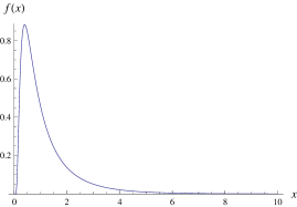
(a) $\theta=0.4$

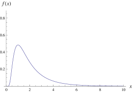
(b) $\theta=1$

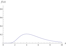
(c) $\theta=4$

Figure 1: Reparameterized inverse Gaussian pdf in (4) with $\gamma=1$.

We now try to clarify the role of $\gamma$. From the standard theory on the IG distribution with pdf given in (1), the variance is $\mu^{3}/\lambda$ (see, e.g., Johnson and Kotz, 1970, Equation (15.6)); thus, thanks to (5), the variance of the random variable $X$ with pdf (4) is

$$\gamma\sqrt{\theta}\sqrt{3\gamma+\theta}.$$

The last expression, analyzed as a function of $\gamma$, is monotone increasing; consequently, fixed $\theta$, the variability increases in line with the value of $\gamma$, confirming that $\gamma$ governs the spread of $X$. The effect of varying $\gamma$, the mode $\theta$ kept fixed, is illustrated in Figure 2.

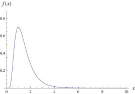
(a) $\gamma=0.4$

(b) $\gamma=1$

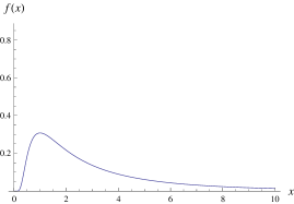
(c) $\gamma=4$

Figure 2: Reparameterized inverse Gaussian pdf in (4) with $\theta=1$.

2.2 Maximum weighted likelihood estimation

Given a sample $x_{1},\ldots,x_{n}$ from the pdf in (4), the weighted log-likelihood function (see, e.g., Skinner et al, 1989, Chapter 3.4.4) related to the rIG distribution is

$$l\left(\theta,\gamma\right)=\sum_{i=1}^{n}w_{i}\ln\left[f\left(x_{i};\theta,\gamma\right)\right],$$ (6)

where $w_{i}\geq 0$, $i=1,\ldots,n$, is a given weight. If $w_{1}=\cdots=w_{n}=1$, then the classical log-likelihood function is obtained. The use of this function is common when data come from surveys as, for example, in the case of the estimation of the income distribution based on household income data (Graf et al, 2011).

The first order partial derivatives of (6) with respect to $\left(\theta,\gamma\right)^{\prime}$ are

$$l^{\prime}\left(\theta,\gamma\right)=\sum_{i=1}^{n}w_{i}\frac{\partial}{\partial\left(\theta,\gamma\right)^{\prime}}\ln\left[f\left(x_{i};\theta,\gamma\right)\right].$$ (7)

Details about the bidimensional vector of the first order partial derivatives on the right-hand side of (7) are given in Appendix A. Similarly, the second order partial derivatives of $l$ with respect to $\left(\theta,\gamma\right)^{\prime}$ are

$$l^{\prime\prime}\left(\theta,\gamma\right)=\sum_{i=1}^{n}w_{i}\frac{\partial^{2}}{\partial\left(\theta,\gamma\right)^{\prime}\partial\left(\theta,\gamma\right)}\ln\left[f\left(x_{i};\theta,\gamma\right)\right].$$ (8)

Details about the symmetric $2\times 2$ matrix of the second order partial derivatives of $\ln\left[f\left(x_{i};\theta,\gamma\right)\right]$, on the right-hand side of (8), are given in Appendix A.

The values of $\theta$ and $\gamma$ that maximize $l\left(\theta,\gamma\right)$ are the maximum weighted likelihood estimates $\widehat{\theta}$ and $\widehat{\gamma}$ and satisfy the condition

$$l^{\prime}\left(\widehat{\theta},\widehat{\gamma}\right)=\boldsymbol{0}.$$

Operationally, we obtain maximization of (6), with respect to $\theta$ and $\gamma$, by the general-purpose optimizer optim() for R (R Core Team, 2016), included in the stats package. The BFGS algorithm, passed to optim() via the argument method, is used for maximization.

3 Applications

In this section we show how our parametrization allows/simplifies the use of the IG distribution in several statistical fields. We define a smoother based on rIG kernels for nonparametric density estimation (Section 3.1), a contaminated IG distribution for robustness in presence of mild outliers (Section 3.2), and a finite mixture of rIG distributions for clustering/classification and semiparametric density estimation (Section 3.3).

3.1 Nonparametric density estimation

Due to their conceptual simplicity and practical and theoretical properties, kernel smoothers are one of the most popular statistical methods for nonparametric density estimation (see, e.g., Silverman, 1986 and Wand and Jones, 1995). Given the random sample $X_{1},\ldots,X_{n}$, these estimators are merely a sum of $n$ (usually symmetric) “bumps” (the so-called kernels), with equal weights $1/n$, placed over each observation. Unfortunately, as stressed in Chen (1999, 2000), while using a symmetric kernel is appropriate for fitting distributions with unbounded supports, it is not adequate for distributions with compact or bounded from one end only supports as it causes boundary bias. The cause of boundary bias is due to the fixed symmetric kernel which allocates weight outside the support when, or especially when (depending from the adopted kernel), smoothing is made near the boundary.

Following the strategy of Punzo (2010, see also , and , ) in the case of finite discrete supports, in Section 3.1.1 we show how a convenient use of rIG kernels automatically permits a solution to boundary bias when the support is $\left(0,\infty\right)$. Moreover, the resulting estimator is well-defined, that is, the produced estimates satisfy all the fundamental properties of a pdf. Section 3.1.2 suggests an objective selection method to select the smoothing parameter of the proposed density estimator.

3.1.1 Reparametrized inverse Gaussian kernel density estimation

Placing a rIG density over each single observation by putting $\theta=X_{i}$ in (4), it is possible to consider the following kernel density smoother

$$\widehat{f}\left(x;\gamma\right)=\frac{1}{n}\sum_{i=1}^{n}f\left(x;\theta=X_{i},\gamma\right)=\frac{1}{n}\sum_{i=1}^{n}k_{\gamma}\left(x;X_{i}\right),\quad 0<x<\infty,$$ (9)

where $k_{\gamma}\left(x;X_{i}\right)$ and $\gamma$ are the rIG kernel and the smoothing parameter, respectively. By construction, (9) defines a density function.

Two quantities characterize the nonparametric estimator (9): the smoothing parameter $\gamma$ and the rIG kernels $k_{\gamma}\left(x;X_{i}\right)$. The former can be considered as smoothing parameter for the following considerations: according to the results of Section 2, if $\gamma$ is chosen too large, then all details, such as modes, may be obscured by $\widehat{f}\left(x;\gamma\right)$. Vice versa, as $\gamma$ becomes small, spurious fine structure becomes visible. The limit as $\gamma\rightarrow 0^{+}$ is a sum of $n$ Dirac delta functions (spikes) over the observations; consequently, $\widehat{f}\left(x;\gamma\right)$ converges to the empirical frequency distribution. As regards the rIG kernels, they obey the fundamental graphical properties of a kernel function. In detail, they are non-negative, integrate to one, assume their maximum value when $x=X_{i}$, and are smoothly non-increasing as the point $x$ departs from $X_{i}$. The only unconventional property is their skewness: indeed, fixed $\gamma$, the kernel shape changes naturally according to the position where the observation $X_{i}$ falls (see Figure 1). In particular, thanks to (5) and recalling (3), the skewness of the density (4) is

$$3\sqrt{\frac{\gamma}{\sqrt{\theta\left(3\gamma+\theta\right)}}};$$ (10)

fixing $\gamma$ in (10), the skewness is a decreasing function of $\theta$. This characteristic, along with the fact that the support $\left(0,\infty\right)$ of a rIG kernel matches the support of the unknown density, constitutes a natural remedy to the problem of boundary bias.

3.1.2 The choice of the smoothing parameter $\gamma$

The smoothing parameter $\gamma$ must be specified and has a dramatic effect on the resulting estimate. Choosing $\gamma$ by trial and error is informative, but it is also convenient to have an objective selection method, and the literature about the topic is vast (see, e.g., Stone, 1974). Amongst the existing methods, cross-validation (CV; Stone, 1974) is without doubt the most commonly used and the simplest to understand. Two common CV alternatives are the least squares CV (LSCV; Silverman, 1986, pp. 48–49) and the likelihood CV (LCV; Silverman, 1986, pp. 52–55). However, as demonstrated by Horne and Garton (2006), LCV generally performs better than LSCV, producing estimates with better fit and less variability, and it is especially beneficial with small sample sizes $n$. Moreover, LCV has general applicability beyond choosing the smooting parameter in kernel density estimation, having been used for both parameter estimation and model selection (see, e.g., Stone, 1974, 1977). The LCV smoothing parameter is chosen by minimizing the score function, suggested by Duin (1976),

$$\text{LCV}\left(\gamma\right)=\frac{1}{n}\sum_{i=1}^{n}\ln\left[\widehat{f}_{-i}\left(x=X_{i};\gamma\right)\right]$$

over the possible values of $\gamma$, where $\widehat{f}_{-i}$ is the density estimate in (9) without the data point $X_{i}$. The value of $\gamma$ that minimizes $\text{CV}\left(\gamma\right)$ is referred to as the LCV smoothing parameter, $\widehat{\gamma}_{\text{LCV}}$. We perform minimization via the nlm() function, of the stats package for R, which carries out a non-linear minimization of $\text{LCV}\left(\gamma\right)$ using a Newton-type algorithm.

3.2 Robustness against mild outliers

Although the IG is one of the most considered distributions with support $\left(0,\infty\right)$, real data are often “contaminated” by outliers — at one or both ends of the support — that can affect the estimation of the parameters. Thus, the detection of outliers, and the development of robust methods of parameter estimation insensitive to their presence, is an important problem.

Outliers can be roughly distinguished into two types (cf. Ritter, 2015, pp. 79–80): mild (also referred to as bad points herein, in analogy with Aitkin and Wilson, 1980) and gross. Mild outliers, on which we focus on, are observations sampled from some population different or even far from the assumed model. Such outliers document mainly the difficulty of the specification problem. In their presence the statistician is recommended to choose a model flexible enough to accommodate all data points, including the outliers. The classical choice is to consider heavy-tailed distributions; endowed with heavy tails, they offer the flexibility needed for achieving mild outliers robustness. Heavy tails are typically obtained by embedding the reference distribution (the IG in our case) in a larger model with one or more additional parameters denoting deviation from the reference distribution due to mild outliers; for a discussion about the concept of reference distribution, see Davies and Gather (1993) and Hennig (2002).

By choosing the rIG as reference distribution, in Section 3.2.1 we propose a simple four-parameter contaminated model in order to accommodate all the available data points. The proposed model is a two-component mixture in which one of the components, with a large prior probability, represents the good points (reference distribution), and the other, with a small prior probability, the same mode, and an inflated parameter $\gamma$, represents the bad points. This is a simple theoretical model for the occurrence of bad points and the two additional parameters, with respect to the parameters of the reference rIG distribution, have a direct interpretation in terms of proportion of good points and degree of contamination (a sort of measure of how different bad points are from the bulk of the good points). Advantageously, the proposed model also allows for automatic detection of bad points via a simple and natural procedure based on maximum a posteriori probabilities. Note that, as we will detail in Section 3.2.1, the parameterization of the IG distribution given in (4) is fundamental for the definition of the contaminated model. We discuss maximum likelihood (ML) estimation of the parameters for the contaminated IG distribution in Section 3.2.2 via the adoption of the expectation-maximization (EM) algorithm.

3.2.1 The contaminated inverse Gaussian distribution

The pdf of the contaminated IG model is given by

$$p\left(x;\theta,\gamma,\alpha,\eta\right)=\alpha f\left(x;\theta,\gamma\right)+\left(1-\alpha\right)f\left(x;\theta,\eta\gamma\right),\quad 0<x<\infty.$$ (11)

In (11):

• $f\left(x;\theta,\gamma\right)$ is the pdf of the rIG, given in (4), chosen as reference distribution.

• $\alpha\in\left(0.5,1\right)$ can be seen as the proportion of good points. Note that $\alpha$ is constrained to be greater than 0.5 because, in robust statistics, it is usually assumed that at least half of the observations are good (cf. Hennig, 2002, p. 250).

• $\eta>1$ denotes the degree of contamination and, because of the assumption $\eta>1$, it can be interpreted as the increase in variability due to the bad points with respect to the reference distribution $f\left(x;\theta,\gamma\right)$; hence, it is an inflation parameter.

Of course, because the reference distribution $f\left(x;\theta,\gamma\right)$ and the inflated distribution $f\left(x;\theta,\eta\gamma\right)$ have their maximum in $\theta$, this also guarantees that $p\left(x;\theta,\gamma,\alpha,\eta\right)$ will produce a unimodal density with mode $\theta$. As a limiting case of (11), when $\alpha\rightarrow 1^{-}$ and $\eta\rightarrow 1^{+}$, the reference distribution $f\left(x;\theta,\gamma\right)$ is obtained.

An advantage of model (11) is that, once $\theta$, $\gamma$, $\alpha$, and $\eta$ are estimated, say $\widehat{\theta}$, $\widehat{\gamma}$, $\widehat{\alpha}$, and $\widehat{\eta}$, we can establish whether a generic data point, say $x^{*}$, is either good or bad via the a posteriori probability

$$P\left(\text{$x^{*}$ is good}\left|\widehat{\theta},\widehat{\gamma},\widehat{\alpha},\widehat{\eta}\right.\right)=\frac{\widehat{\alpha}f\left(x^{*};\widehat{\theta},\widehat{\gamma}\right)}{p\left(x^{*};\widehat{\theta},\widehat{\gamma},\widehat{\alpha},\widehat{\eta}\right)}.$$ (12)

Based on (12), $x^{*}$ will be considered good if $P\left(\text{$x^{*}$ is good}\left|\widehat{\theta},\widehat{\gamma},\widehat{\alpha},\widehat{\eta}\right.\right)>1/2$, while it will be considered bad otherwise. The resulting information can be used to eliminate the bad points, if such an outcome is desired (Berkane and Bentler, 1988).

3.2.2 Maximum likelihood estimation: An EM algorithm

In analogy with Section 2.2, estimates of the parameters $\theta$, $\gamma$, $\alpha$, and $\eta$ can be determined by the maximization of the weighted log-likelihood function if sample weights $w_{1},\ldots,w_{n}$ are available in addition to the sample $x_{1},\ldots,x_{n}$ from model (11). Details about the four first order partial derivatives of $\ln\left[p\left(x;\theta,\gamma,\alpha,\eta\right)\right]$ are given in Appendix B for the reader interested in this approach.

Below, to find classical ML estimates of the parameters, we illustrate the use of the EM algorithm (Dempster et al, 1977), which is a natural approach for ML estimation when data are incomplete. In our case, the source of missing data arises from the fact that we do not know whether the generic data point $x_{i}$, $i=1,\ldots,n$, is good or bad. To denote this source of missing data, we use the indicator variables $v_{1},\ldots,v_{i},\ldots,v_{n}$, where $v_{i}=1$ if $x_{i}$ is good and $v_{i}=0$ otherwise, $i=1,\ldots,n$. Therefore, the complete-data are given by $\left(x_{1},v_{1}\right),\ldots,\left(x_{i},v_{i}\right),\ldots,\left(x_{n},v_{n}\right)$ and the complete-data likelihood, on which the algorithm works on, can be written as

$$L_{c}\left(\theta,\gamma,\alpha,\eta\right)=\prod_{i=1}^{n}\left[\alpha f\left(x_{i};\theta,\gamma\right)\right]^{v_{i}}\left[\left(1-\alpha\right)f\left(x_{i};\theta,\eta\gamma\right)\right]^{1-v_{i}}.$$

Simple algebra yields the following complete-data log-likelihood

$$l_{c}\left(\theta,\gamma,\alpha,\eta\right)=l_{1c}\left(\alpha\right)+l_{2c}\left(\theta,\gamma,\eta\right),$$ (13)

where

$$l_{1c}\left(\alpha\right)=\sum_{i=1}^{n}\left[v_{i}\ln\alpha+\left(1-v_{i}\right)\ln\left(1-\alpha\right)\right]$$ (14)

and

$$l_{2c}\left(\theta,\gamma,\eta\right)=\sum_{i=1}^{n}\left[v_{i}\ln f\left(x_{i};\theta,\gamma\right)+\left(1-v_{i}\right)\ln f\left(x_{i};\theta,\eta\gamma\right)\right].$$ (15)

The EM algorithm iterates between two steps, one E-step and one M-step, until convergence. We implement the EM algorithm in R.

E-step

The E-step, on the $\left(r+1\right)$th iteration of the EM algorithm, requires the calculation of $Q\left(\theta,\gamma,\alpha,\eta\right)$, the current conditional expectation of $l_{c}\left(\theta,\gamma,\alpha,\eta\right)$. To do this, we need to calculate $E\left(V_{i}|x_{i};\theta^{\left(r\right)},\gamma^{\left(r\right)},\alpha^{\left(r\right)},\eta^{\left(r\right)}\right)$, where $V_{i}$ is the random variable related to $v_{i}$, $i=1,\ldots,n$; this expectation is given by

$$E\left(V_{i}|x_{i};\theta^{\left(r\right)},\gamma^{\left(r\right)},\alpha^{\left(r\right)},\eta^{\left(r\right)}\right)=\frac{\alpha^{\left(r\right)}f\left(x_{i};\theta^{\left(r\right)},\gamma^{\left(r\right)}\right)}{p\left(x_{i};\theta^{\left(r\right)},\gamma^{\left(r\right)},\alpha^{\left(r\right)},\eta^{\left(r\right)}\right)}\eqqcolon v_{i}^{\left(r\right)},$$

which is the posterior probability that $x_{i}$ is a good point; compare with (12). Then, by substituting $v_{i}$ with $v_{i}^{\left(r\right)}$ in (13), and based on (14) and (15), we obtain $Q\left(\theta,\gamma,\alpha,\eta\right)=Q_{1}\left(\alpha\right)+Q_{2}\left(\theta,\gamma,\eta\right)$.

M-step

The M-step on the $\left(r+1\right)$th iteration of the EM algorithm requires the calculation of $\theta^{\left(r+1\right)}$, $\gamma^{\left(r+1\right)}$, $\alpha^{\left(r+1\right)}$, and $\eta^{\left(r+1\right)}$ as the values of $\theta$, $\gamma$, $\alpha$, and $\eta$ that maximize $Q\left(\theta,\gamma,\alpha,\eta\right)$. The update for $\alpha$ is calculated independently by maximizing

$$Q_{1}\left(\alpha\right)=\sum_{i=1}^{n}\left[v_{i}^{\left(r\right)}\ln\alpha+\left(1-v_{i}^{\left(r\right)}\right)\ln\left(1-\alpha\right)\right]$$

with respect to $\alpha$, subject to the constraint on this parameter. Some simple algebra yields

$$\alpha^{\left(r+1\right)}=\max\left\{0.5,\frac{1}{n}\sum_{i=1}^{n}v_{i}^{\left(r\right)}\right\}.$$

The updates of $\theta$, $\gamma$, and $\eta$ are obtained by the maximization of the function

$$Q_{2}\left(\theta,\gamma,\eta\right)=\sum_{i=1}^{n}\left[v_{i}^{\left(r\right)}\ln f\left(x_{i};\theta,\gamma\right)+\left(1-v_{i}^{\left(r\right)}\right)\ln f\left(x_{i};\theta,\eta\gamma\right)\right].$$ (16)

For R users, the optim() function, in the stats package, can be used to perform a numerical search of the maximum $(\theta^{\left(r+1\right)},\gamma^{\left(r+1\right)},\eta^{\left(r+1\right)})^{\prime}$ of the function (16).

3.3 Model-based clustering and semiparametric density estimation

Finite mixtures of distributions are commonly employed in statistical modeling for two different purposes (Titterington et al, 1985, pp. 2–3). In indirect applications, they are used as semiparametric competitors of nonparametric density estimation techniques (Titterington et al, 1985, pp. 28–29, McLachlan and Peel, 2000, p. 8, and Escobar and West, 1995). On the other hand, in direct applications, finite mixture models are considered a powerful device for clustering/classification by assuming that each mixture component represents a group (or cluster) in the original data (see McLachlan and Basford, 1988). A wide range of disciplines can benefit from the application of mixture models, from biology and medicine (Schlattmann, 2009) to economics and marketing (Wedel and Kamakura, 2000); overviews are given in McLachlan and Peel (2000), Frühwirth-Schnatter (2006), and McNicholas (2016).

Most of the work published is concerned with mixtures of Gaussian distributions; they are able to approximate arbitrarily well any continuous distribution (see, e.g., McLachlan and Peel, 2000, p. 1). Although using Gaussian components in the mixture is in principle appropriate when the theoretical support is , it is not adequate if the support is $\left(0,\infty\right)$ due to the boundary bias issue discussed in Section 3.1. A simple remedy is to use mixture components defined on $\left(0,\infty\right)$. Motivated by this consideration, we suggest using rIG components. The choice of rIG components is justified, but above all natural, if one thinks that the most striking feature of a mixture density is often that of multimodality. Indeed, as highlighted in Titterington et al (1985) and McLachlan and Basford (1988), many papers in applied fields talk not in terms of mixtures but of multimodal distributions; examples are the articles by Murphy (1964) and Brazier et al (1983) referring to bimodality rather than to mixtures.

3.3.1 Mixtures of reparametrized inverse Gaussian distributions

The finite mixture of rIG densities can be written as

$$p\left(x;\boldsymbol{\pi},\boldsymbol{\theta},\boldsymbol{\gamma}\right)=\sum_{j=1}^{k}\pi_{j}f\left(x;\theta_{j},\gamma_{j}\right),\quad 0<x<\infty.$$ (17)

In (17)

• $f\left(x;\theta_{j},\gamma_{j}\right)$ is the rIG component density with parameters $\theta_{j}$ and $\gamma_{j}$;

• $\boldsymbol{\pi}=\left(\pi_{1},\ldots,\pi_{k}\right)^{\prime}$ is the vector of mixture weights, with $\pi_{j}\in\left(0,1\right)$ and $\sum_{j=1}^{k}\pi_{j}=1$;

• $\boldsymbol{\theta}=\left(\theta_{1},\ldots,\theta_{k}\right)^{\prime}$ is the vector of component modes $\theta_{j}$;

• $\boldsymbol{\gamma}=\left(\gamma_{1},\ldots,\gamma_{k}\right)^{\prime}$ is the vector of component parameters $\gamma_{j}$.

Thus, there are $3k-1$ unknown parameters to be estimated. Of course, as also underlined by Izenman (2008, p. 103) and Bagnato and Punzo (2013), there is no guarantee that $p$ will produce a multimodal density with the same number of modes as there are densities in the mixture; similarly, there is no guarantee that those individual modes $\theta_{j}$ will remain at the same locations in (17). Indeed, the shape of the mixture distribution depends upon both the spacings of the modes and the relative shapes of the component distributions. Nevertheless, we retain that for well-separated components, the values of $\theta_{j}$ should accurately approximate the location of the mixture modes.

In terms of indirect applications, model (17) provides a semiparametric compromise between the single (parametric) rIG density given in (4), in the case $k=1$, and the nonparametric method of density estimation based on rIG kernels given in (9), in the case $k=n$.

3.3.2 Maximum likelihood estimation: The EM algorithm

As for the contaminated IG distribution, to find ML estimates of the parameters for model (17) we use the EM algorithm. In this case the source of incompleteness, the classical one in the use of mixture models, arises from the fact that for each observation we do not know its component membership; this source, which is especially related to a direct application of the model, is governed by an indicator vector $\boldsymbol{z}_{i}=\left(z_{i1},\ldots,z_{ik}\right)$, where $z_{ij}=1$ if $x_{i}$ comes from component $j$ and $z_{ij}=0$ otherwise. The complete-data likelihood can be written as

$$L_{c}\left(\boldsymbol{\pi},\boldsymbol{\theta},\boldsymbol{\gamma}\right)=\prod_{i=1}^{n}\prod_{j=1}^{k}\left[\pi_{j}f\left(x_{i};\theta_{j},\gamma_{j}\right)\right]^{z_{ij}}.$$

Therefore, the complete-data log-likelihood becomes

$$l_{c}\left(\boldsymbol{\pi},\boldsymbol{\theta},\boldsymbol{\gamma}\right)=l_{1c}\left(\boldsymbol{\pi}\right)+l_{2c}\left(\boldsymbol{\theta},\boldsymbol{\gamma}\right),$$ (18)

where

$$l_{1c}\left(\boldsymbol{\pi}\right)= \sum_{i=1}^{n}\sum_{j=1}^{k}{z}_{ij}\ln\pi_{j},$$ (19)

$$l_{2c}\left(\boldsymbol{\theta},\boldsymbol{\gamma}\right)= \sum_{i=1}^{n}\sum_{j=1}^{k}z_{ij}\ln\left[f\left(x_{i};\theta_{j},\gamma_{j}\right)\right].$$ (20)

E-step and M-step are described below.

E-step

The E-step, on the $\left(r+1\right)$th iteration of the EM algorithm, requires the calculation of $Q\left(\boldsymbol{\pi},\boldsymbol{\theta},\boldsymbol{\gamma}\right)$, the current conditional expectation of $l_{c}\left(\boldsymbol{\pi},\boldsymbol{\theta},\boldsymbol{\gamma}\right)$. To do this, we need to calculate

$$E\left(Z_{ij}|x_{i};\boldsymbol{\pi}^{\left(r\right)},\boldsymbol{\theta}^{\left(r\right)},\boldsymbol{\gamma}^{\left(r\right)}\right)=\frac{\pi_{j}^{\left(r\right)}f\left(x_{i};\theta_{j}^{\left(r\right)},\gamma_{j}^{\left(r\right)}\right)}{p\left(x_{i};\boldsymbol{\pi}^{\left(r\right)},\boldsymbol{\theta}^{\left(r\right)},\boldsymbol{\gamma}^{\left(r\right)}\right)}\eqqcolon z_{ij}^{\left(r\right)}.$$

Then, by substituting $z_{ij}$ with $z_{ij}^{\left(r\right)}$ in (18), and based on (19) and (20), we obtain

$$Q\left(\boldsymbol{\pi},\boldsymbol{\theta},\boldsymbol{\gamma}\right)=Q_{1}\left(\boldsymbol{\pi}\right)+Q_{2}\left(\boldsymbol{\theta},\boldsymbol{\gamma}\right).$$ (21)

M-step

The M-step on the $\left(r+1\right)$th iteration of the EM algorithm requires the calculation of $\boldsymbol{\pi}^{\left(r+1\right)}$, $\boldsymbol{\theta}^{\left(r+1\right)}$, and $\boldsymbol{\gamma}^{\left(r+1\right)}$ as the values of $\boldsymbol{\pi}$, $\boldsymbol{\theta}$, and $\boldsymbol{\gamma}$ that maximize $Q\left(\boldsymbol{\pi},\boldsymbol{\theta},\boldsymbol{\gamma}\right)$. As the two terms on the right-hand side of (21) have zero cross-derivatives, they can be maximized separately. Maximizing $Q_{1}\left(\boldsymbol{\pi}\right)$ with respect to $\boldsymbol{\pi}$, subject to the constraints on these parameters, yields

$$\pi_{j}^{\left(r+1\right)}=\frac{1}{n}\sum_{i=1}^{n}z_{ij}^{\left(r\right)},\quad j=1,\ldots,k.$$

Maximizing $Q_{2}\left(\boldsymbol{\theta},\boldsymbol{\gamma}\right)$ with respect to $\boldsymbol{\theta}$ and $\boldsymbol{\gamma}$ (subject to the constraints on these parameters), is equivalent to independently maximizing each of the $k$ expressions

$$Q_{2j}\left(\theta_{j},\gamma_{j}\right)=\sum_{i=1}^{n}z_{ij}^{\left(r\right)}\ln\left[f\left(x_{i};\theta_{j},\gamma_{j}\right)\right],\quad j=1,\ldots,k.$$

$Q_{2j}\left(\theta_{j},\gamma_{j}\right)$ is a weighted log-likelihood, with weights $z_{ij}^{\left(r\right)}$, $i=1,\ldots,n$, whose maximization has been discussed in Section 2.2.

4 Real data analysis

In this section we will show how the rIG-based models, introduced in Section 3, act on real data coming from different disciplines.

4.1 Bodily injury claims

The first example comes from the insurance world. As well-known insurance data are often positive, right-skewed, and leptokurtic (Ibragimov et al, 2015). Several parametric families of distributions have been considered in the literature to accommodate these peculiarities, including the Pareto, Weibull, log-normal, and gamma distributions (Klugman et al, 2012). However, when insurance data exhibit unusual shapes, such as multiple modes, these distributions may not be a good candidate, as well-argued in Lee and Lin (2010) and Jeon and Kim (2013). In these cases, a more flexible modelling framework, such as a mixture modelling framework, is to be preferred. The flexibility of finite mixtures in accommodating various shapes of insurance data is now widely recognized (Choy and Chan, 2003, Bernardi et al, 2012, Choy et al, 2016, and Maruotti et al, 2016). Among them, mixtures of gamma distributions were successfully considered in Dey et al (1995), Wiper et al (2001), and Venturini et al (2008). As we will see in the analysis below, mixtures of rIG distributions, introduced in Section 3.3, represent a valid alternative.

We use insurance data from Rempala and Derrig (2005), which are also available in the CASdatasets package (Dutang and Charpentier, 2016) for R. The sample represents the bodily injury claims from Massachusetts closed in 2001. We consider the $n=272$ claims that are coded as “other providers”, thus ignoring potentially fraudulent claims; all numbers are in thousand dollars as in the original paper.

The histogram of the data, displayed in Figure 3, shows multimodality and right-skewness.

Figure 3: Bodily injury claims. Histogram together with a rIG-kernel density estimator.

To further explore the characteristics of the empirical pdf, we compute the rIG kernel density estimator introduced in Section 3.1. The smoothing parameter, selected according to the likelihood cross-validation method discussed in Section 3.1.2, is $\widehat{\gamma}_{\text{LCV}}=0.431$; the corresponding solid curve is superimposed on the histogram in Figure 3. The nonparametric curve confirms the multimodality suggested by the histogram giving prominence to a clear bimodality.

Motivated by these preliminary findings, we fit mixtures of unimodal gamma distributions (Bagnato and Punzo, 2013) and mixtures of rIG distributions (introduced in Section 3.3) with a number $k$ of mixture components ranging from 1 to 4. Each model is fitted via the EM algorithm. To allow for a direct comparison of the competing models, all the algorithms are initialized by providing the initial quantities $\boldsymbol{z}_{i}^{(0)}$, $i=1,\ldots,n$, to the first M-step: 9 times using a random initialization and once with a $k$-means initialization (as implemented by the kmeans() function for R). The solution maximizing the observed-data log-likelihood among these 10 runs is then selected; see Dang et al (2017). We select the best value of $k$, as usual in the mixture modelling literature, via the Bayesian information criterion (BIC; Schwarz, 1978). Even though the regularity properties needed for the development of the BIC are not satisfied by mixture models (Keribin, 1998, 2000), it has been used extensively (see, e.g., Dasgupta and Raftery, 1998 and Fraley and Raftery, 2002) and performs well in practice. We compute the BIC as

$$\text{BIC}=2l\left(\widehat{\boldsymbol{\pi}},\widehat{\boldsymbol{\theta}},\widehat{\boldsymbol{\gamma}}\right)-\left(3k-1\right)\ln n,$$

where $l\left(\widehat{\boldsymbol{\pi}},\widehat{\boldsymbol{\theta}},\widehat{\boldsymbol{\gamma}}\right)$ is the maximized (observed-data) log-likelihood. Note that, Bayes factors can be used to compare models that are not nested, and the BIC approximation thereto holds when models are not nested (cf. Raftery, 1995).

Table 1 shows the obtained BIC values.

Table 1: Bodily injury claims. BIC values for the fitted models. Bold numbers refer to the best value of $k$ for each model.

		1	2	3	4
mixt. of gamma pdfs		-1093.122	-1066.879	-1033.998	-1049.733
mixt. of rIG pdfs		-1169.075	-1026.641	-1031.266	-1046.069

The BIC suggests $k=3$ components for mixtures of gamma distributions and $k=2$ components for mixtures of rIG distributions. These results confirm the observation that a single ($k=1$) parametric model – gamma or rIG in our case – is unable to represent the distribution of the bodily injury claims. Overall, the best model is the mixture of two rIG distributions; its estimated parameters are given in Table 2, while its graphical representation is displayed, via a solid line, in Figure 4, with dotted curves showing the component densities multiplied by the corresponding estimated weights $\widehat{\pi}_{j}$, $j=1,2$. Group membership of the observations is represented by ticks of different colors (black for group 1 and gray for group 2) on the $x$-axis.

Table 2: Bodily injury claims. Estimated parameters for the mixture of two rIG distributions.

		$\widehat{\pi}_{j}$	$\widehat{\theta}_{j}$	$\widehat{\gamma}_{j}$
1		0.507	0.175	11.901
2		0.493	2.527	0.262

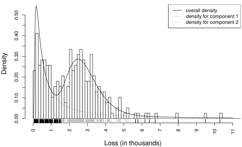
Figure 4: Bodily injury claims. Histogram together with the fitted mixture of $k=2$ rIG densities. Dotted lines show the component densities multiplied by the corresponding weights. Black and gray are used for observations in group 1 and group 2, respectively, as classified by the fitted model.

This application emphasizes the importance of the mode-parameterization, which immediately gives an idea of the location, on the $x$-axis, of the losses with the highest probability (see the third column of Table 2). In particular, the first mode suggests that a loss of 175 dollars is the most likely for this dataset. Moreover, the estimated modes can be used to facilitate comparisons across space and time of the two losses more representative of the distribution.

4.2 Income of Italian households in 1986

The second example comes from the economic literature and it is related to the estimation of the income distribution. Information from such estimation is used to measure welfare, inequality and poverty, to assess changes in these measures over time, and to compare measures across countries, over time and before and after specific policy changes, designed, for example, to alleviate poverty. Thus, the estimation of the income distribution is of central importance for assessing many aspects of the well being of society (see Silber, 2012, for further considerations).

The income distribution has been estimated both parametrically and nonparametrically (see, e.g., Chotikapanich and Griffiths, 2008). Parametric estimation is convenient because it facilitates subsequent inferences about inequality and poverty measures based on the estimated income distribution parameters. A large number of alternative parametric models have been suggested in the literature for estimating the income distribution (see Kleiber and Kotz, 2003, for a survey). As well documented in Dagum (2008), a convenient parametric model should be: defined on a strictly positive support, unimodal, and positively skewed; moreover, all the parameters of the specified model should have a well-defined economic meaning and, following a principle of parsimony, the model should make use of the smallest possible number of parameters for adequate and meaningful representation. Unfortunately, as emphasized by Van Praag et al (1983), Feser (1993), and Cowell and Victoria-Feser (1996), real income data are often “contaminated” by outliers (bad incomes) that affect the estimation of the parameters for the chosen model. This in turn will affect the inequality measure computed from the estimated parameters. As we will see in the analysis below, the contaminated IG distribution can be a remedy to this problem.

We use incomes of Italian households, for 1986, obtained from the Luxembourg Income Study (LIS) database (http://www.lisdatacenter.org/). The data analyzed here are $n=6016$ household incomes with corresponding sample weights. The weighted histogram of the data, obtained via the function wtd.hist() of the weights package (Pasek, 2016) for R, is displayed in Figure 5. Although, as expected, the histogram highlights unimodality and positive skewness, some spurious very high incomes appear (see the ticks on the $x$-axis) yielding an heavier right tail.

Figure 5: Income of Italian households in 1986. Weighted histogram.

Motivated by these considerations, we fit the rIG and the contaminated IG distributions to data at hand. Their nested relationship guarantees that the contaminated IG distribution will fit the data at least as well as the rIG distribution. However, this superiority could not be statistically significant. Thanks to the nested relationship between the competing models, a natural way to compare their goodness-of-fit consists of using the likelihood-ratio (LR) statistic

$$\text{LR}=2\left[l\left(\widehat{\theta},\widehat{\gamma},\widehat{\alpha},\widehat{\eta}\right)-l\left(\widehat{\theta},\widehat{\gamma}\right)\right],$$

where $l\left(\widehat{\theta},\widehat{\gamma},\widehat{\alpha},\widehat{\eta}\right)$ and $l\left(\widehat{\theta},\widehat{\gamma}\right)$ are the maximized (observed-data) log-likelihoods for the contaminated and uncontaminated IG models, respectively. Under the null hypothesis that the true underlying model is the restricted one (the rIG in our case), versus the alternative that the true underlying model is the more complex one (the contaminated IG in our case), LR is asymptotically distributed as a $\chi^{2}$ with two degrees of freedom, corresponding to the difference in the number of free parameters between the null and the alternative model. Thus, from a practical point of view, the degrees of freedom can be seen as the gain in parsimony that could be obtained using the model under the null instead of the model under the alternative. With data at hand, the LR statistic assumes value 59.455, and the resulting $p$-value is $1.229\times 10^{-13}$, which leads to the rejection of the null, in favor of the alternative, at any reasonable significance level.

The estimated parameters for the contaminated IG distribution are $\widehat{\theta}=5.389$, $\widehat{\gamma}=6.179$, $\widehat{\alpha}=0.991$, and $\widehat{\eta}=15.726$. The estimated value of $\alpha$ indicates that about the 9‰ of the incomes can be considered as bad according to the fitted model, with $\widehat{\eta}$ giving the degree of badness (measure of how far the bad incomes are from the bulk of the data). The corresponding estimated curve is represented, via a solid line, in Figure 6, along with the weighted histogram; dotted curves show the densities for good and bad incomes multiplied by the corresponding estimated weights $\widehat{\alpha}$ and $1-\widehat{\alpha}$. Maximum a posteriori classification of incomes, as good or bad, is represented by ticks of different colors (gray for good incomes and black for bad incomes) on the $x$-axis.

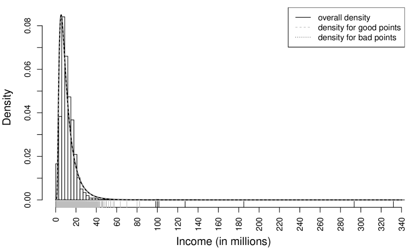
Figure 6: Income of Italian households in 1986. Weighted histogram together with the fitted contaminated IG density (solid line). Dotted lines show the densities for good and bad incomes multiplied by the corresponding weights. Gray and black are used for good and bad incomes, respectively, as classified by the fitted model.

Figure 7 reports, for each income $x_{i}$, the estimated posterior probability in (12) to be good, $i=1,\ldots,n$; as we can see, the farther the income is from the bulk of the data, as represented by the mode $\widehat{\theta}$, the lower is its probability to be a good income. Such probability is also related to the down-weighting of bad incomes in the estimation of the model parameters, and this is an important aspect for robust estimation (see Punzo and McNicholas, 2016 for a discussion about this topic with reference to the mixture of contaminated normal distributions).

Figure 7: Income of Italian households in 1986. Estimated posterior probabilities to be good incomes. Gray and black are used for good and bad incomes, respectively, as classified by the fitted model.

5 Conclusions

A mode-based parameterization of the inverse Gaussian (IG) distribution was suggested. It yielded the reparametrized IG (rIG) distribution. It was used to define three different models to be applied for positive data: a rIG kernel smoother for nonparametric density estimation (Section 3.1), a contaminated IG distribution for robust density estimation (Section 3.2), and a finite mixture of rIG distributions for clustering and semiparametric density estimation (Section 3.3). The real data applications illustrated in Section 4 showed the usefulness of the proposed models.

However, the applicability of our parameterization is not restricted to the models discussed above. For example, the rIG could be used as distribution of the error term in modal linear regression (Yao and Li, 2014); the modal linear regression models the conditional mode of a response $Y$ given a set of predictors $\boldsymbol{x}$ as a linear function of $\boldsymbol{x}$. Also, in the fashion of Punzo and McNicholas (2016), contaminated IG distributions may be used as components in the definition of a finite mixture model; see also Punzo et al (2017), Punzo and McNicholas (2017), Punzo and Maruotti (2016), and Maruotti and Punzo (2017). Finally, in reliability theory, the parameterization with respect to the mode may simplify the formulation of the hazard rate, related to the IG distribution (cf. Seshadri, 2012, Chapter 5.3).

Appendix A Partial derivatives of the log pdf of the rIG distribution

The first order partial derivatives with respect to $\theta$ and $\gamma$, of the logarithm of the pdf in (4), are

$$\frac{\partial\ln\left[f\left(x;\theta,\gamma\right)\right]}{\partial\theta}=-\frac{3}{2x}-\frac{\theta}{x\gamma}+\frac{1}{3\gamma+\theta}+\frac{3\gamma}{2\theta(3\gamma+\theta)}+\frac{\sqrt{\theta}}{2\gamma\sqrt{3\gamma+\theta}}+\frac{\sqrt{3\gamma+\theta}}{2\gamma\sqrt{\theta}}$$

and

$$\frac{\partial\ln\left[f\left(x;\theta,\gamma\right)\right]}{\partial\gamma}=\frac{x}{2\gamma^{2}}+\frac{\theta^{2}}{2x\gamma^{2}}-\frac{\theta}{2\gamma(3\gamma+\theta)}+\frac{3\sqrt{\theta}}{2\gamma\sqrt{3\gamma+\theta}}-\frac{\sqrt{\theta\left(3\gamma+\theta\right)}}{\gamma^{2}}.$$

The second order partial derivatives are

$$\frac{\partial^{2}\ln\left[f\left(x;\theta,\gamma\right)\right]}{\partial\theta^{2}}=-\frac{1}{4}\left(\frac{4}{x\gamma}+\frac{2}{\theta^{2}}+\frac{2}{(3\gamma+\theta)^{2}}+\frac{9\gamma}{\theta^{3/2}(3\gamma+\theta)^{3/2}}\right),$$

$$\frac{\partial^{2}\ln\left[f\left(x;\theta,\gamma\right)\right]}{\partial\theta\partial\gamma} =\frac{\partial^{2}\ln\left[f\left(x;\theta,\gamma\right)\right]}{\partial\gamma\partial\theta}$$

$$=\frac{\theta}{x\gamma^{2}}+\frac{-27\gamma^{3}-30\gamma\theta^{2}-4\theta^{3}-3\gamma^{2}\left[21\theta+2\sqrt{\theta\left(3\gamma+\theta\right)}\right]}{4\gamma^{2}\sqrt{\theta}(3\gamma+\theta)^{5/2}},$$

and

$$\frac{\partial^{2}\ln\left[f\left(x;\theta,\gamma\right)\right]}{\partial\gamma^{2}}= -\frac{x}{\gamma^{3}}-\frac{\theta^{2}}{x\gamma^{3}}+\frac{3\theta}{2\gamma(3\gamma+\theta)^{2}}-\frac{9\sqrt{\theta}}{4\gamma(3\gamma+\theta)^{3/2}}+\frac{\theta}{2\gamma^{2}(3\gamma+\theta)}$$

$$-\frac{3\sqrt{\theta}}{\gamma^{2}\sqrt{3\gamma+\theta}}+\frac{2\sqrt{\theta\left(3\gamma+\theta\right)}}{\gamma^{3}}.$$

Appendix B First partial derivatives of the log pdf of the contaminated IG distribution

The first order partial derivatives with respect to $\theta$, $\gamma$, $\alpha$, and $\eta$ of the logarithm of the pdf in (11), are

$$\frac{\partial\ln\left[p\left(x;\theta,\gamma,\alpha,\eta\right)\right]}{\partial\theta}=\frac{1}{2\sqrt{2\pi}\gamma^{2}x^{4}p\left(x;\theta,\gamma,\alpha,\eta\right)}\times$$

$$\quad\left[\frac{\alpha\left(3\gamma+2\theta\right)\left\{x\left[\gamma+\sqrt{\theta\left(3\gamma+\theta\right)}\right]-\theta\left(3\gamma+\theta\right)\right\}\exp\left\{-\frac{\left[x-\sqrt{\theta\left(3\gamma+\theta\right)}\right]^{2}}{2x\gamma}\right\}}{\sqrt{\frac{\theta\left(3\gamma+\theta\right)}{x^{3}\gamma}}}\right.+$$

$$\quad\left.\frac{\left(1-\alpha\right)\left(3\eta\gamma+2\theta\right)\left\{x\left[\eta\gamma+\sqrt{\theta\left(3\eta\gamma+\theta\right)}\right]-\theta\left(3\eta\gamma+\theta\right)\right\}\exp\left\{-\frac{\left[x-\sqrt{\theta\left(3\eta\gamma+\theta\right)}\right]^{2}}{2x\eta\gamma}\right\}}{\eta^{2}\sqrt{\frac{\theta\left(3\eta\gamma+\theta\right)}{x^{3}\eta\gamma}}}\right],$$

$$\frac{\partial\ln\left[p\left(x;\theta,\gamma,\alpha,\eta\right)\right]}{\partial\gamma}=\frac{\theta}{2\sqrt{2\pi}\gamma^{3}x^{4}p\left(x;\theta,\gamma,\alpha,\eta\right)}\times$$

$$\quad\qquad\left[\frac{x^{2}\left(3\gamma+\theta\right)+\theta^{2}\left(3\gamma+\theta\right)-x\left[\gamma\theta+3\gamma\sqrt{\theta\left(3\gamma+\theta\right)}+2\theta\sqrt{\theta\left(3\gamma+\theta\right)}\right]}{\sqrt{\frac{\theta\left(3\gamma+\theta\right)}{x^{3}\gamma}}}\right.\times$$

$$\quad\qquad\alpha\exp\left\{-\frac{\left[x-\sqrt{\theta\left(3\gamma+\theta\right)}\right]^{2}}{2x\gamma}\right\}+\left(1-\alpha\right)\exp\left\{-\frac{\left[x-\sqrt{\theta\left(3\eta\gamma+\theta\right)}\right]^{2}}{2x\eta\gamma}\right\}\times$$

$$\quad\qquad\left.\frac{x^{2}\left(3\eta\gamma+\theta\right)+\theta^{2}\left(3\eta\gamma+\theta\right)-x\left[2\theta\sqrt{\theta\left(3\eta\gamma+\theta\right)}+\eta\gamma\left(\theta+3\sqrt{\theta\left(3\eta\gamma+\theta\right)}\right)\right]}{\eta^{2}\sqrt{\frac{\theta\left(3\eta\gamma+\theta\right)}{x^{3}\eta\gamma}}}\right],$$

$$\frac{\partial\ln\left[p\left(x;\theta,\gamma,\alpha,\eta\right)\right]}{\partial\alpha}=$$

$$\qquad\frac{\sqrt{\frac{\theta\left(3\gamma+\theta\right)}{x^{3}\gamma}}\exp\left\{-\frac{\left[x-\sqrt{\theta\left(3\eta\gamma+\theta\right)}\right]^{2}}{2x\eta\gamma}\right\}-\sqrt{\frac{\theta\left(3\eta\gamma+\theta\right)}{x^{3}\eta\gamma}}\exp\left\{-\frac{\left[x-\sqrt{\theta\left(3\gamma+\theta\right)}\right]^{2}}{2x\gamma}\right\}}{\alpha\sqrt{\frac{\theta\left(3\gamma+\theta\right)}{x^{3}\gamma}}\exp\left\{-\frac{\left[x-\sqrt{\theta\left(3\eta\gamma+\theta\right)}\right]^{2}}{2x\eta\gamma}\right\}+\left(1-\alpha\right)\sqrt{\frac{\theta\left(3\eta\gamma+\theta\right)}{x^{3}\eta\gamma}}\exp\left\{-\frac{\left[x-\sqrt{\theta\left(3\gamma+\theta\right)}\right]^{2}}{2x\gamma}\right\}},$$

and

$$\frac{\partial\ln\left[p\left(x;\theta,\gamma,\alpha,\eta\right)\right]}{\partial\eta}=\frac{\exp\left\{-\frac{\left[x-\sqrt{\theta\left(3\gamma+\theta\right)}\right]^{2}}{2x\gamma}\right\}}{2x^{4}\gamma^{2}\eta^{3}\frac{\theta(3\eta\gamma+\theta)}{\sqrt{x^{3}\eta\gamma}}}\times$$

$$\qquad\frac{\left(1-\alpha\right)\left(\left(x^{2}+\theta^{2}\right)\left[\theta\left(3\eta\gamma+\theta\right)\right]^{3/2}-x\theta^{2}\left\{9\gamma^{2}\eta^{2}+2\theta^{2}+\eta\gamma\left[9\theta+\sqrt{\theta\left(3\eta\gamma+\theta\right)}\right]\right\}\right)}{\alpha\sqrt{\frac{\theta\left(3\gamma+\theta\right)}{x^{3}\gamma}}\exp\left\{-\frac{\left[x-\sqrt{\theta\left(3\eta\gamma+\theta\right)}\right]^{2}}{2x\eta\gamma}\right\}+\left(1-\alpha\right)\sqrt{\frac{\theta\left(3\eta\gamma+\theta\right)}{x^{3}\eta\gamma}}\exp\left\{-\frac{\left[x-\sqrt{\theta\left(3\gamma+\theta\right)}\right]^{2}}{2x\gamma}\right\}}.$$

References

- Aitkin and Wilson (1980) Aitkin M, Wilson GT (1980) Mixture models, outliers, and the EM algorithm. Technometrics 22(3):325–331
- Bagnato and Punzo (2013) Bagnato L, Punzo A (2013) Finite mixtures of unimodal beta and gamma densities and the -bumps algorithm. Computational Statistics 28(4):1571–1597
- Berkane and Bentler (1988) Berkane M, Bentler PM (1988) Estimation of contamination parameters and identification of outliers in multivariate data. Sociological Methods & Research 17(1):55–64
- Bernardi et al (2012) Bernardi M, Maruotti A, Petrella L (2012) Skew mixture models for loss distributions: A bayesian approach. Insurance: Mathematics and Economics 51:617–623
- Brazier et al (1983) Brazier S, Sparks RSJ, Carey SN, Sigurdsson H, Westgate JA (1983) Bimodal Grain Size Distribution and Secondary Thickening in Air-Fall Ash Layers. Nature 301:115–119
- Chen (1999) Chen SX (1999) Beta kernel estimators for density functions. Computational Statistics & Data Analysis 31(2):131–145
- Chen (2000) Chen SX (2000) Probability density function estimation using gamma kernels. Annals of the Institute of Statistical Mathematics 52(3):471–480
- Chhikara and Folks (1988) Chhikara RS, Folks JL (1988) The Inverse Gaussian Distribution: Theory, Methodology, and Applications, Statistics: A Series of Textbooks and Monographs, vol 95. Taylor & Francis, New York
- Chotikapanich and Griffiths (2008) Chotikapanich D, Griffiths WE (2008) Estimating income distributions using a mixture of gamma densities. In: Chotikapanich D (ed) Modeling Income Distributions and Lorenz Curves, Economic Studies in Inequality, Social Exclusion and Well-Being, Springer, New York, chap 16, pp 285–302
- Choy et al (2016) Choy SB, Chan JS, Makov UE (2016) Robust bayesian analysis of loss reserving data using scale mixtures distributions. Journal of Applied Statistics 43(3):396–411
- Choy and Chan (2003) Choy STB, Chan CM (2003) Scale mixtures distributions in insurance applications. ASTIN Bulletin 33(1):93–104
- Cowell and Victoria-Feser (1996) Cowell FA, Victoria-Feser MP (1996) Robustness properties of inequality measures. Econometrica 64(1):77–101
- Dagum (2008) Dagum C (2008) A new model of personal income distribution: Specification and estimation. In: Chotikapanich D (ed) Modeling Income Distributions and Lorenz Curves, Economic Studies in Equality, Social Exclusion and Well-Being, vol 5, Springer, New York, chap 1, pp 3–25
- Dang et al (2017) Dang UJ, Punzo A, McNicholas PD, Ingrassia S, Browne RP (2017) Multivariate response and parsimony for Gaussian cluster-weighted models. Journal of Classification 34(1):4–34
- Dasgupta and Raftery (1998) Dasgupta A, Raftery AE (1998) Detecting features in spatial point processes with clutter via model-based clustering. Journal of the American Statistical Association 93(441):294–302
- Davies and Gather (1993) Davies L, Gather U (1993) The identification of multiple outliers. Journal of the American Statistical Association 88(423):782–792
- Dempster et al (1977) Dempster AP, Laird NM, Rubin DB (1977) Maximum likelihood from incomplete data via the EM algorithm. Journal of the Royal Statistical Society: Series B (Statistical Methodology) 39(1):1–38
- Dey et al (1995) Dey DK, Kuo L, Sahu SK (1995) A bayesian predictive approach to determining the number of components in a mixture distribution. Statistics and Computing 5(4):297–305
- Duin (1976) Duin RPW (1976) On the choice of smoothing parameters for parzen estimators of probability density functions. IEEE Transactions on Computers 25(11):1175–1179
- Dutang and Charpentier (2016) Dutang C, Charpentier A (2016) CASdatasets: Insurance datasets (Official website). URL http://cas.uqam.ca/, version 1.0-6 (2016-05-28)
- Escobar and West (1995) Escobar MD, West M (1995) Bayesian density estimation and inference using mixtures. Journal of the American Statistical Association 90(430):577–588
- Feser (1993) Feser MPV (1993) Robust estimation of personal income distribution models. Research Paper DARP/4, London School of Economics and Political Science
- Folks and Chhikara (1978) Folks JL, Chhikara RS (1978) The inverse Gaussian distribution and its statistical application–a review. Journal of the Royal Statistical Society: Series B (Statistical Methodology) 40(3):263–289
- Fraley and Raftery (2002) Fraley C, Raftery AE (2002) Model-based clustering, discriminant analysis, and density estimation. Journal of the American Statistical Association 97(458):611–631
- Frühwirth-Schnatter (2006) Frühwirth-Schnatter S (2006) Finite Mixture and Markov Switching Models. Springer, New York
- Graf et al (2011) Graf M, Nedyalkova D, Müunnich R, Seger J, Zins S (2011) Parametric estimation of income distributions and indicators of poverty and social exclusion. European Research Project Report WP2 - D2.1, FP7-SSH-2007-217322 AMELI (Advanced Methodology for European Laeken Indicators), European Commission funding from the Seventh Framework Programme for Research, available at: www.uni-trier.de/fileadmin/fb4/projekte/SurveyStatisticsNet/Ameli_Delivrables/AMELI-WP2-D2.1-20110409.pdf
- Hennig (2002) Hennig C (2002) Fixed point clusters for linear regression: computation and comparison. Journal of Classification 19(2):249–276
- Horne and Garton (2006) Horne JS, Garton EO (2006) Likelihood cross-validation versus least squares cross-validation for choosing the smoothing parameter in kernel home-range analysis. Journal of Wildlife Management 70(3):641–648
- Ibragimov et al (2015) Ibragimov M, Ibragimov R, Walden J (2015) Heavy-Tailed Distributions and Robustness in Economics and Finance, Lecture Notes in Statistics, vol 214. Springer International Publishing, New York
- Izenman (2008) Izenman AJ (2008) Modern Multivariate Statistical Techniques: Regression, Classification, and Manifold Learning. Springer, New York
- Jeon and Kim (2013) Jeon Y, Kim JHT (2013) A gamma kernel density estimation for insurance loss data. Insurance: Mathematics and Economics 53:569–579
- Johnson and Kotz (1970) Johnson NL, Kotz S (1970) Continuous Univariate Distributions, vol 1. John Wiley & Sons, New York
- Keribin (1998) Keribin C (1998) Estimation consistante de l’ordre de modèles de mélange. Comptes Rendus de l’Académie des Sciences-Series I-Mathematics 326(2):243–248
- Keribin (2000) Keribin C (2000) Consistent estimation of the order of mixture models. Sankhyā: The Indian Journal of Statistics, Series A 62:49–66
- Kleiber and Kotz (2003) Kleiber C, Kotz S (2003) Statistical Size Distributions in Economics and Actuarial Sciences, Wiley Series in Probability and Statistics, vol 470. John Wiley & Sons, New York
- Klugman et al (2012) Klugman SA, Panjer HH, Willmot GE (2012) Loss Models: From Data to Decisions. Wiley Series in Probability and Statistics, Wiley
- Lee and Lin (2010) Lee SCK, Lin XS (2010) Modeling and evaluating insurance losses via mixtures of Erlang distributions. North American Actuarial Journal 14(1):107–130
- Maruotti and Punzo (2017) Maruotti A, Punzo A (2017) Model-based time-varying clustering of multivariate longitudinal data with covariates and outliers. Computational Statistics & Data Analysis 113:475–496
- Maruotti et al (2016) Maruotti A, Raponi V, Lagona F (2016) Handling endogeneity and nonnegativity in correlated random effects models: Evidence from ambulatory expenditure. Biometrical Journal 58(2):280–302
- Mazza and Punzo (2011) Mazza A, Punzo A (2011) Discrete beta kernel graduation of age-specific demographic indicators. In: Ingrassia S, Rocci R, Vichi M (eds) New Perspectives in Statistical Modeling and Data Analysis, Springer-Verlag, Berlin Heidelberg, Studies in Classification, Data Analysis and Knowledge Organization, pp 127–134
- Mazza and Punzo (2013a) Mazza A, Punzo A (2013a) Graduation by adaptive discrete beta kernels. In: Giusti A, Ritter G, Vichi M (eds) Classification and Data Mining, Springer-Verlag, Berlin Heidelberg, Studies in Classification, Data Analysis and Knowledge Organization, pp 243–250
- Mazza and Punzo (2013b) Mazza A, Punzo A (2013b) Using the variation coefficient for adaptive discrete beta kernel graduation. In: Giudici P, Ingrassia S, Vichi M (eds) Statistical Models for Data Analysis, Springer International Publishing, Switzerland, Studies in Classification, Data Analysis and Knowledge Organization, pp 225–232
- Mazza and Punzo (2014) Mazza A, Punzo A (2014) DBKGrad: An R package for mortality rates graduation by discrete beta kernel techniques. Journal of Statistical Software 57(Code Snippet 2):1–18
- Mazza and Punzo (2015) Mazza A, Punzo A (2015) Bivariate discrete beta kernel graduation of mortality data. Lifetime Data Analysis 21(3):419–433
- McLachlan and Basford (1988) McLachlan GJ, Basford KE (1988) Mixture Models: Inference and Applications to Clustering. Statistics: A Series of Textbooks and Monographs, Marcel Dekker, New York
- McLachlan and Peel (2000) McLachlan GJ, Peel D (2000) Finite Mixture Models. John Wiley & Sons, New York
- McNicholas (2016) McNicholas PD (2016) Mixture Model-Based Classification. Chapman and Hall/CRC Press, Boca Raton
- Murphy (1964) Murphy EA (1964) One Cause? Many Causes? The Argument from the Bimodal Distribution. Journal of Chronic Diseases 17(4):301–324
- Pasek (2016) Pasek J (2016) weights: Weighting and Weighted Statistics. URL https://cran.r-project.org/web/packages/weights/index.html, version 0.85 (2016-02-12)
- Punzo (2010) Punzo A (2010) Discrete beta-type models. In: Locarek-Junge H, Weihs C (eds) Classification as a Tool for Research, Springer-Verlag, Berlin Heidelberg, Studies in Classification, Data Analysis and Knowledge Organization, pp 253–261
- Punzo and Maruotti (2016) Punzo A, Maruotti A (2016) Clustering multivariate longitudinal observations: The contaminated Gaussian hidden Markov model. Journal of Computational and Graphical Statistics 25(4):1097–1116
- Punzo and McNicholas (2016) Punzo A, McNicholas PD (2016) Parsimonious mixtures of multivariate contaminated normal distributions. Biometrical Journal 58(6):1506–1537
- Punzo and McNicholas (2017) Punzo A, McNicholas PD (2017) Robust clustering in regression analysis via the contaminated Gaussian cluster-weighted model. Journal of Classification 34(2), DOI 10.1007/s00357-017-9234-x
- Punzo and Zini (2012) Punzo A, Zini A (2012) Discrete approximations of continuous and mixed measures on a compact interval. Statistical Papers 53(3):563–575
- Punzo et al (2017) Punzo A, Mazza A, McNicholas PD (2017) ContaminatedMixt: An R package for fitting parsimonious mixtures of multivariate contaminated normal distributions. Journal of Statistical Software pp 1–25
- R Core Team (2016) R Core Team (2016) R: A Language and Environment for Statistical Computing. R Foundation for Statistical Computing, Vienna, Austria, URL https://www.R-project.org/
- Raftery (1995) Raftery AE (1995) Bayesian model selection in social research. Sociological Methodology 25:111–164
- Rempala and Derrig (2005) Rempala GA, Derrig RA (2005) Modeling hidden exposures in claim severity via the EM algorithm. North American Actuarial Journal 9(2):108–128
- Ritter (2015) Ritter G (2015) Robust Cluster Analysis and Variable Selection, Chapman & Hall/CRC Monographs on Statistics & Applied Probability, vol 137. CRC Press
- Schlattmann (2009) Schlattmann P (2009) Medical Applications of Finite Mixture Models. Statistics for Biology and Health, Springer-Verlag, Berlin Heidelberg
- Schwarz (1978) Schwarz G (1978) Estimating the dimension of a model. The Annals of Statistics 6(2):461–464
- Seshadri (2012) Seshadri V (2012) The Inverse Gaussian Distribution: Statistical Theory and Applications, Lecture Notes in Statistics, vol 137. Springer, New York
- Silber (2012) Silber J (2012) Handbook of Income Inequality Measurement, Recent Economic Thought, vol 71. Springer, Netherlands
- Silverman (1986) Silverman BW (1986) Density Estimation for Statistics and Data Analysis. Chapman & Hall/CRC, London
- Skinner et al (1989) Skinner CJ, Holt D, Smith TMF (1989) Analysis of Complex Surveys. Wiley Series in Probability and Mathematical Statistics, Wiley
- Stone (1974) Stone M (1974) Cross-validatory choice and assessment of statistical predictions. Journal of the Royal Statistical Society: Series B (Statistical Methodology) 36(1):111–147
- Stone (1977) Stone M (1977) An asymptotic equivalence of choice of model by cross-validation and Akaike’s criterion. Journal of the Royal Statistical Society: Series B (Statistical Methodology) 39(1):44–47
- Titterington et al (1985) Titterington DM, Smith AFM, Makov UE (1985) Statistical Analysis of Finite Mixture Distributions. John Wiley & Sons, New York
- Tweedie (1957) Tweedie MCK (1957) Statistical properties of inverse Gaussian distributions. I. The Annals of Mathematical Statistics 28(2):362–377
- Van Praag et al (1983) Van Praag B, Hagenaars A, Van Eck W (1983) The influence of classification and observation errors on the measurement of income inequality. Econometrica 51(4):1093–1108
- Venturini et al (2008) Venturini S, Dominici F, Parmigiani G (2008) Gamma shape mixtures for heavy-tailed distributions. The Annals of Applied Statistics 2(2):756–776
- Wand and Jones (1995) Wand MP, Jones MC (1995) Kernel Smoothing. Chapman & Hall Ltd
- Wedel and Kamakura (2000) Wedel M, Kamakura W (2000) Market Segmentation: Conceptual and Methodological Foundations, 2nd edn. Kluwer Academic Publishers, Boston, MA, USA
- Wiper et al (2001) Wiper M, Insua DR, Ruggeri F (2001) Mixtures of gamma distributions with applications. Journal of Computational and Graphical Statistics 10(3):440–454
- Yao and Li (2014) Yao W, Li L (2014) A new regression model: modal linear regression. Scandinavian Journal of Statistics 41(3):656–671