Comprehensive Analysis on Exact Asymptotics of
Random Coding Error Probability

Abstract

This paper considers error probabilities of random codes for memoryless channels in the fixed-rate regime. Random coding is a fundamental scheme to achieve the channel capacity and many studies have been conducted for the asymptotics of the decoding error probability. Gallager derived the exact asymptotics (that is, a bound with asymptotically vanishing relative error) of the error probability for fixed rate below the critical rate. On the other hand, exact asymptotics for rate above the critical rate has been unknown except for symmetric channels (in the strong sense) and strongly nonlattice channels. This paper derives the exact asymptotics for general memoryless channels covering all previously unsolved cases. The analysis reveals that strongly symmetric channels and strongly nonlattice channels correspond to two extreme cases and the expression of the asymptotics is much complicated for general channels.

I Introduction

Random coding is a fundamental scheme in many problems of information theory and asymptotically achieves the capacity in channel coding. This code is also important in the finite block length regime to clarify the achievable performance of channel codes. For this purpose Polyanskiy [1] and Hayashi [2] considered random codes with varying coding rate for fixed error probability and revealed that loss in the coding rate from the capacity is $\mathrm{O}(1/\sqrt{n})$ for the block length $n$.

Whereas these bounds are convenient for evaluate the error probability with small absolute error, it is sometimes useful to evaluate the error probability with small relative error when the acceptable error probability is very small. This line of work is closely related to the theory of error exponent, which considers exponential decay of the error probability for fixed rate $R$. Gallager [3] derived an upper bound of the error probability of random coding called a random coding union bound. It is shown that the use of union bound does not worsen the exponent for coding rates below the critical rate [3] and above the critical rate [4].

As a higher-order analysis for the error exponent, there are many studies to evaluate the random coding error probability $P_{\mathrm{RC}}(n)$ with vanishing relative error for fixed coding rate $R$ and block length $n$ for memoryless channels. Dobrushin [5] showed that the random coding error probability is written in a form $\Theta(n^{-a(R)}\mathrm{e}^{-nE(R)})$ for discrete symmetric channels in the strong sense that each row and the column of the transition probability matrix are permutations of the others. They also derived the specific value of $\lim_{n\to\infty}n^{a(R)}\mathrm{e}^{E(R)}P_{\mathrm{RC}}(n)$ for the nonlattice case (defined later) and noted that the limit does not exist for some cases.

For general class of discrete memoryless channels, Gallager [6] showed that the upper bound derived in [3] is also the lower bound with vanishing relative error for rate below the critical rate. Altuğ and Wagner [7] corrected his result for singular channels. They, and Scarlett et al. [8], also derived upper bounds of the error probability for general rate $R$. However these bounds, denoted by $\hat{P}(n)$, do not assure $\hat{P}(n)/P_{\mathrm{RCU}}(n)=\Omega(1)$ although $\hat{P}(n)/P_{\mathrm{RCU}}(n)=\mathrm{O}(1)$ is proved.

Honda [9] derived a framework to evaluate the random coding error probability for general (possibly nondiscrete) nonsingular memoryless channels. He introduced a two-dimensional random variable, which will be denoted by $(Z(\eta),Z^{\prime}(\eta))$ or $(Z_{0},Z_{1})$ for short, and showed that $\lim_{n\to\infty}\mathrm{E}[f_{n}(\bar{Z}_{0},\bar{Z}_{1})]/P_{\mathrm{RC}}(n)=1$ for some function $f_{n}$, where $(\bar{Z}_{0},\bar{Z}_{1})$ is the empirical mean of $n$ i.i.d. copies of $(Z_{0},Z_{1})$. Thus, we can obtain an explicit representation of $P_{\mathrm{RC}}(n)$ if $\mathrm{E}[f_{n}(\bar{Z}_{0},\bar{Z}_{1})]$ is approximated appropriately. It is known that the error of normal approximation of $(\bar{Z}_{0},\bar{Z}_{1})$ becomes large if Cramér’s condition is not satisfied, or equivalently, if $(Z_{0},Z_{1})$ is distributed over a lattice or a set of parallel lines with equal interval. In these cases the analysis becomes much complicated and Honda [9] only derived an explicit representation of $\mathrm{E}[f_{n}(\bar{Z}_{0},\bar{Z}_{1})]$ for the case that Cramér’s condition is satisfied. For continuous channels such as Gaussian channels lattice distributions do not appear and a higher-order analysis is given in [10].

In this paper we derive simple representation of $\mathrm{E}[f_{n}(\bar{Z}_{0},\bar{Z}_{1})]$, or equivalently $P_{\mathrm{RC}}(n)$, for general $(Z_{0},Z_{1})$ including the case that $(Z_{0},Z_{1})$ is distributed over a lattice or parallel lines, which is the last region where the exact asymptotics of the random coding error probability has been unknown for singular channels. Our analysis reveals that strongly symmetric channels considered in [5] belong to the degenerate case that $Z_{1}$ is a linear deterministic function of $Z_{0}$ and the asymptotic form of the error probability becomes much simpler. We also derive the exact asymptotics for singular channels by applying the same techniques. Thus our analysis covers all previously unknown cases in the evaluation of random coding error probability with vanishing relative gap for fixed rate $R$.

The main difficulty of the derivation is that the required precision for the evaluation of $(Z_{0},Z_{1})$ is not “isotropic”. More precisely, $\mathrm{E}[f_{n}(\bar{Z}_{0},\bar{Z}_{1})]$ depends on the behavior of $\bar{Z}_{0}$ in $\mathrm{o}(1/\sqrt{n})$ precision whereas $\mathrm{E}[f_{n}(\bar{Z}_{0},\bar{Z}_{1})]$ has rough dependence on $\bar{Z}_{1}$ and $\mathrm{o}(1/\sqrt{n})$ precision for $\bar{Z}_{2}$ does not lead to a simple expression. Based on this observation, we start with local limit theorem for $(\bar{Z}_{0},\bar{Z}_{1})$ with $\mathrm{o}(1/\sqrt{n})$ precision in both directions and “blur” the distribution function only in $\bar{Z}_{1}$ direction.

II Preliminary

We consider a memoryless channel with input alphabet $\mathcal{X}$ and output alphabet $\mathcal{Y}$. The output distribution for input $x\in\mathcal{X}$ is denoted by $W(\cdot|x)$. Let $X\in\mathcal{X}$ be a random variable with distribution $P_{X}$ and $Y\in\mathcal{Y}$ follow $W(\cdot|X)$ given $X$. $X^{\prime}$ is a random variable with the same distribution as $X$ and independent of $(X,Y)$. $(\bm{X},\bm{Y},\bm{X}^{\prime})=((X_{1},\cdots,X_{n}),\,(Y_{1},\cdots,Y_{n}),\,(X_{1}^{\prime},\cdots,X_{n}^{\prime}))$ denotes $n$ independent copies of $(X,Y,X^{\prime})$.

We assume that there exists a base measure $Q$ such that $W(\cdot|x)$ is absolutely continuous with respect to $Q$ for all $x$. Under this assumption, we also use $W(y|x)$ to denote the Radon-Nikodym derivative $\frac{\mathrm{d}W(\cdot|x)}{\mathrm{d}Q}(y)$ by a slight abuse of notation. Since the density satisfies $W(Y|X)>0$ almost surely, the log likelihood ratio

$$\nu(X,Y,x^{\prime})=\log\frac{W(Y|x^{\prime})}{W(Y|X)}\in[-\infty,\infty)$$

is well-defined almost surely for any $x^{\prime}\in\mathcal{X}$. We assume that the mutual information is finite, that is, $I(X;Y)=\mathrm{E}_{XY}[-\log\mathrm{E}_{X^{\prime}}[\mathrm{e}^{\nu(X,Y,X^{\prime})}]]<\infty$.

We consider the error probability of a random code such that each element of codewords $(\bm{X}_{1},\cdots,\allowbreak\bm{X}_{M})\in\mathcal{X}^{n\times M}$ is generated independently from distribution $P_{X}$. The coding rate of this code is given by $R=(\log M)/n$. We use the maximum likelihood decoding

$$\hat{\bm{X}}=\operatorname*{\rm argmax}_{j\in\{1,2,\cdots,M\}}\sum_{i=1}^{n}\log W(Y_{i}|(\bm{X}_{j})_{i})\,.$$

We mainly consider the case that ties are broken uniformly at random. See Sect. V for ties immediately regarded as a decoding error. Note that the former case corresponds to [5] and the latter case is considered in [6].

For a random variable $V$ we write $\bar{V}$ to denote the empirical mean of $n$ i.i.d. copies and write $\tilde{V}=\sqrt{n}(\bar{V}-\mathrm{E}[\bar{V}])$. We write $a\land b=\min\{a,b\}$ and $a\lor b=\max\{a,b\}$. For $x=0$ we define $(\mathrm{e}^{x}-1)/x=x/(\mathrm{e}^{x}-1)=1$.

II-A Error Exponent

Define a random variable $Z(\lambda)$ on the space of functions $\mathbb{R}\to\mathbb{R}$ by

$$Z(\lambda) =\log\mathrm{E}_{X^{\prime}}\left[\mathrm{e}^{\lambda\nu(X,Y,X^{\prime})}\right]$$

and its derivatives by

$$Z^{(m)}(\lambda) =\frac{\mathrm{d}^{m}}{\mathrm{d}\lambda^{m}}\log\mathrm{E}_{X^{\prime}}\left[\mathrm{e}^{\lambda\nu(X,Y,X^{\prime})}\right]\,,$$

which we also write as $Z^{\prime}(\lambda),\,Z^{\prime\prime}(\lambda),\cdots$. Here $\mathrm{E}_{X^{\prime}}$ denotes the expectation over $X^{\prime}$ for given $(X,Y)$. We define

$$Z(\lambda+\mathrm{i}\xi) =\log\mathrm{E}_{X^{\prime}}\left[\mathrm{e}^{(\lambda+\mathrm{i}\xi)\nu(X,Y,X^{\prime})}\right]$$

$${Z_{\mathrm{a}}}(\lambda+\mathrm{i}\xi) =\log\left|\mathrm{E}_{X^{\prime}}\left[\mathrm{e}^{(\lambda+\mathrm{i}\xi)\nu(X,Y,X^{\prime})}\right]\right|\,,$$

where $\lambda,\xi\in\mathbb{R}$ and $\mathrm{i}$ is the imaginary unit. Here we always consider the case $\lambda>0$ and define $\mathrm{e}^{(\lambda+\mathrm{i}\xi)(-\infty)}=0$.

The random coding error exponent for $0<R<I(X;Y)$ is denoted by

$$E_{r}(R) =-\inf_{(\alpha,\lambda)\in[0,1]\times[0,\infty)}\{\alpha R+\log\mathrm{E}[\mathrm{e}^{\alpha Z(\lambda)}]\}$$

$$=-\min_{\alpha\in(0,1]}\{\alpha R+\log\mathrm{E}[\mathrm{e}^{\alpha Z(1/(1+\alpha))}]\}\,,$$ (1)

and we write the optimal solution of $(\alpha,\lambda)$ as $(\rho,\eta)=(\rho,1/(1+\rho))$. Critical rate $R_{\mathrm{crit}}$ is the largest $R$ such that the optimal solution of (1) is $\rho=1$.

In the strict sense the random coding error exponent represents the supremum of (1) over $P_{X}$ but for simplicity we fix $P_{X}$ and omit its dependence. See [7, Theorem 2] for a condition that there exists $P_{X}$ which attains this supremum.

Let $P_{\rho}$ be the probability measure such that $\mathrm{d}P_{\rho}/\mathrm{d}P=\mathrm{e}^{\rho Z(\eta)-\mathrm{\Lambda}(\rho)}$ for $\mathrm{\Lambda}(\rho)=\log\mathrm{E}[\mathrm{e}^{\rho Z(1/(1+\rho))}]$. We write the expectation under $P_{\rho}$ by $\mathrm{E}_{\rho}$ and define

$$\mu_{i} =\mathrm{E}_{\rho}[Z^{(i)}(\eta)]=\mathrm{e}^{-\mathrm{\Lambda}(\rho)}\mathrm{E}[Z^{(i)}(\eta)\mathrm{e}^{\rho Z(\eta)}]$$

$$\sigma_{ij} =\mathrm{E}_{\rho}[(Z^{(i)}(\eta)-\mu_{i})(Z^{(j)}(\eta)-\mu_{j})]$$

$$=\mathrm{e}^{-\mathrm{\Lambda}(\rho)}\mathrm{E}[(Z^{(i)}(\eta)-\mu_{i})(Z^{(j)}(\eta)-\mu_{j})\mathrm{e}^{\rho Z(\eta)}]$$

$$\Sigma =\left(\begin{array}[]{cc}\sigma_{00}&\sigma_{01}\\ \sigma_{10}&\sigma_{11}\end{array}\right)\,.$$ (4)

By letting $\Delta=-(\mu_{0}+R)$ we have $\Delta>0$ if $R<R_{\mathrm{crit}}$ and $\Delta=0$ otherwise. For a one-dimensional random variable $V\in\underline{\mathbb{R}}$, we say that $V$ is singular if $V\in\{-\infty,v\}$ a.s. for some $v\in\mathbb{R}$.

Definition 1.

Channel $W$ is singular if $\nu(X,Y,X^{\prime})$ given $(X,Y)$ is singular almost surely, that is, $P_{X^{\prime}}[\nu(X,Y,X^{\prime})\in\{-\infty,0\}]=1$ a.s.

As discussed in [5], $\mu_{2}=0$ if $W$ is singular and $\mu_{2}>0$ otherwise.

II-B Lattice and Nonlattice Distributions

We call that nonsingular one-dimensional random variable $V\in\underline{\mathbb{R}}$ has a lattice distribution with span $h>0$ and offset $a\in\mathbb{R}$ if $V\in\{a+ih:i\in\mathbb{Z}\}\cup\{-\infty\}$ a.s. and $h$ is the largest one satisfying this property.

Let $a\in\mathbb{R}^{2}$ be arbitrary and $h^{(1)},h^{(2)}\in\mathbb{R}^{2}$ be linearly independent vectors. We say that two-dimensional random variable $V\in\mathbb{R}^{2}$ with covariance matrix $\Sigma$ satisfying $|\Sigma|\neq 0$ has a lattice distribution over $L=\{a+ih^{(1)}+jh^{(2)}:i,j\in\mathbb{Z}\}$ if $V\in L$ a.s. and no sublattice of $L$ satisfies this property. We say that $V\in\mathbb{R}^{2}$ has a lattice-nonlattice distribution over set $L^{\prime}=\{a+ih^{(1)}+th^{(2)}:i\in\mathbb{Z},t\in\mathbb{R}\}$ of lines with equal interval if $V\in L^{\prime}$ a.s. and $(h^{(1)},h^{(2)})$ is a pair with largest $|\det(h^{(1)},h^{(2)})|/\|h^{(2)}\|$. We say that $V\in\mathbb{R}^{2}$ has a strongly nonlattice distribution if $V$ does not have a lattice distribution or lattice-nonlattice distribution.

Definition 2.

Channel $W$ is $h$-lattice if $\nu(X,Y,X^{\prime})$ has a lattice distribution with span $h$ and is nonlattice otherwise. We define the span of a nonlattice channel as $h=0$.

Note that if $W$ is $h$-lattice then the offset of $\nu(X,Y,X^{\prime})$ is zero from the definition of $\nu$. Whereas this classification of a channel also appears in many studies such as [6], we also consider another classification to derive a tight bound. This classification also depends on $\eta=1/(1+\rho)$ that is determined from $R$.

Definition 3.

Channel and rate pair $(W,R)$ is $(h^{\prime},a^{\prime})$-lattice if $Z(\eta)$ has a lattice distribution with span $h^{\prime}$ and offset $a^{\prime}$, and is nonlattice otherwise. The pair $(W,R)$ is pseudo-symmetric if $(Z(\eta),Z^{\prime}(\eta))$ is distributed over some single line, that is, $Z^{\prime}(\eta)$ is a linear function of $Z(\eta)$.

Dobrushin [5] considered the case that $W$ is a symmetric discrete channel in the strong sense that each row and column of the transition probability matrix are permutations of the others. In this case the conditional distribution of $W(Y|X^{\prime})$ given $Y$ does not depend on $Y$ and therefore for any $y_{0}\in\mathcal{Y}$ we have

$$Z(\eta) =\log\mathrm{E}_{X^{\prime}}[W(y_{0}|X^{\prime})^{\eta}]-\eta\log W(Y|X)\,,$$

$$Z^{\prime}(\eta) =\frac{\mathrm{E}_{X^{\prime}}[W(y_{0}|X^{\prime})^{\eta}\log W(y_{0}|X^{\prime})]}{\mathrm{E}_{X^{\prime}}[W(y_{0}|X^{\prime})^{\eta}]}-\log W(Y|X)\,.$$

The first terms of RHSs of them are constants and the following property trivially holds.

Proposition 1.

Assume that discrete channel $W$ is strongly symmetric. Then $(W,R)$ is pseudo-symmetric for any $R$. Furthermore, $W$ is $h$-lattice if and only if $(W,R)$ is $(\eta h,a)$-lattice for some $a\in\mathbb{R}$.

We can see from this proposition that symmetric channels considered in [5] correspond to the degenerate case where $(Z(\eta),Z^{\prime}(\eta))$ is linearly dependent.

As in [9] we always assume that for lattice span $h\geq 0$ of $W$ there exist $\alpha,b_{0}>0$ and a neighborhood $\mathcal{S}\ni\lambda$ of $\eta$ such that for any $0<b_{1}<b_{2}<2\pi/h\leq\infty$

$$\sup_{\lambda\in\mathcal{S}}\mathrm{E}_{\rho}[\mathrm{e}^{\alpha|Z^{(i)}(\lambda)|}]<\infty\,,\quad i=1,2,3,$$

$$\sup_{\lambda\in\mathcal{S},\,\xi\in[-b_{0},b_{0}]}\mathrm{E}_{\rho}[\mathrm{e}^{\alpha|(\partial^{4}/\partial\xi^{4})Z(\lambda+\mathrm{i}\xi)|}]<\infty\,,$$

$$\sup_{\lambda\in\mathcal{S},\,\xi\in[b_{1},b_{2}]}\mathrm{E}_{\rho}[\mathrm{e}^{\alpha|{Z_{\mathrm{a}}}(\lambda+\mathrm{i}\xi)-{Z_{\mathrm{a}}}(\lambda)|}]<\infty\,,$$

which are trivially satisfied for finite discrete channels.

III Exact Asymptotics for Nonsingular Channels

In this section we derive the exact asymptotics for nonsingular channels covering results in [5][9] as special cases. First we give the exact asymptotics for $R\leq R_{\mathrm{crit}}$.

Theorem 1.

Let $W$ be a channel with lattice span $h\geq 0$ of $W$. Then

$$P_{\mathrm{RC}}(n)=\begin{cases}\frac{(1+\mathrm{o}(1))h(\mathrm{e}^{h/2}+1)}{2(\mathrm{e}^{h/2}-1)\sqrt{2\pi n(\mu_{2}+\sigma_{11})}}\mathrm{e}^{-nE_{r}(R)},&\mbox{if $R<R_{\mathrm{crit}}$},\\ \frac{(1+\mathrm{o}(1))h(\mathrm{e}^{h/2}+1)}{4(\mathrm{e}^{h/2}-1)\sqrt{2\pi n(\mu_{2}+\sigma_{11})}}\mathrm{e}^{-nE_{r}(R)},&\mbox{if $R=R_{\mathrm{crit}}$}.\end{cases}$$ (5)

We prove this theorem in Appendix B using two-dimensional Berry-Esseen bound (or one-dimensional one for pseudo-symmetric $(W,R)$) in [11].

The derived bound is equal to those of [6] (for $R<R_{\mathrm{crit}}$) and [5] (for strongly symmetric channels) when $W$ is nonlattice, whereas these three bounds are different to each other for the lattice case. Gallager [6] derived a bound for ties regarded as errors and the bound in this theorem for uniformly broken ties is slightly smaller than the bound in [6] as discussed in Sect. V. On the other hand, Dobrushin [5] considered uniformly broken ties but the explicit expression on the constant factor was not derived for this case.

Now we consider the case $R>R_{\mathrm{crit}}$. In this case the bound also depends on whether $(W,R)$ is lattice or not and becomes much complicated. For $h\geq 0$, let

$$g_{h}(u) =1-\frac{\mathrm{e}^{-\frac{h\eta}{\mathrm{e}^{h\eta}-1}u}(1-\mathrm{e}^{-h\eta u})}{h\eta u}$$

$$g_{\rho,h}(u) =u^{-\rho}g_{h}(u)=\frac{1}{u^{\rho}}-\frac{\mathrm{e}^{-\frac{h\eta}{\mathrm{e}^{h\eta}-1}u}(1-\mathrm{e}^{-h\eta u})}{h\eta u^{1+\rho}}$$

$$\psi_{\rho,h,h^{\prime}}(x) =\sum_{i\in\mathbb{Z}}h^{\prime}g_{\rho,h}(\mathrm{e}^{x+ih^{\prime}})$$

$$\psi_{\rho,h} =\int_{w\in\mathbb{R}}g_{\rho,h}(\mathrm{e}^{w})\mathrm{d}w$$

$$=\frac{\Gamma(1-\rho)}{\rho}\left(\frac{h\eta}{\mathrm{e}^{h\eta}-1}\right)^{\rho+1}\frac{\mathrm{e}^{h}-1}{h}\,,$$ (6)

where $\Gamma(\cdot)$ is Gamma function. Note that $\psi_{\rho,h,h^{\prime}}(x)$ is a periodic function with period $h^{\prime}$ and satisfies $\psi_{\rho,h}=\lim_{h^{\prime}\downarrow 0}\psi_{\rho,h,h^{\prime}}(x)$ for any $x\in\mathbb{R}$. The following theorem is the main contribution of this paper, which solves the exact asymptotics of random coding error probability for rate above the critical rate.

Theorem 2.

Fix $R\in(R_{\mathrm{crit}},I(X;Y))$ and let $h>0$ be the lattice span of channel $W$. Then

$$P_{\mathrm{RC}}(n)=(1+\mathrm{o}(1))\frac{(1+\rho)^{\rho}I_{n}}{\sqrt{(2\pi)^{1+\rho}\mu_{2}^{\rho}}}n^{-(1+\rho)/2}\mathrm{e}^{-nE(R)}\,,$$

where, if $(W,R)$ is nonlattice then

$$I_{n} =I=\frac{\psi_{\rho,h}}{\sqrt{\sigma_{00}+\rho|\Sigma|/\mu_{2}}}$$ (7)

and if $(W,R)$ is $(h^{\prime},a^{\prime})$-lattice then

$$I_{n} =\frac{\mathrm{E}_{V}\left[\psi_{\rho,h,h^{\prime}}\left(na^{\prime}-\frac{|\Sigma|V^{2}}{2(\sigma_{00}+\rho|\Sigma|/\mu_{2})}-\log c_{2}\sqrt{n}\right)\right]}{\sqrt{\sigma_{00}+\rho|\Sigma|/\mu_{2}}}$$ (8)

for standard normal $V$. In particular, if $(W,R)$ is pseudo-symmetric then

$$\!\!\!\!I_{n}=\begin{cases}\frac{\psi_{\rho,h}}{\sqrt{\sigma_{00}}},&\mbox{$(W,R)$ is nonlattice,}\\ \frac{\psi_{\rho,h,h^{\prime}}\left(na^{\prime}-\log c_{2}\sqrt{n}\right)}{\sqrt{\sigma_{00}}},&\mbox{$(W,R)$ is $(h^{\prime},a^{\prime})$-lattice.}\\ \end{cases}$$ (9)

We give a sketch of a proof in Sect. VI and the full proof is in Appendix C. If $(W,R)$ is pseudo-symmetric then $|\Sigma|=0$ and the bound (9) is a special case of (7) and (8), although the proof is given separately.

The bound in [9] for strongly nonlattice $(Z(\eta),Z^{\prime}(\eta))$ is a special case of (7). If $(W,R)$ is lattice then $P_{\mathrm{RC}}(n)\cdot\allowbreak n^{(1+\rho)/2}\mathrm{e}^{nE(R)}$ does not converge as shown in this theorem. This phenomenon is suggested in [5] for strongly symmetric channel, which is a special case of pseudo-symmetric $(W,R)$. Furthermore, if $(W,R)$ is not pseudo-symmetric then $P_{\mathrm{RC}}(n)n^{(1+\rho)/2}\mathrm{e}^{nE(R)}$ is expressed as an expectation of a periodic function for a normal random variable, which seems to be impossible to integrate out analytically. The known bounds are summarized in Fig. 1 and the derived bound in this paper covers all region.

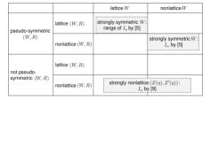
Figure 1: Known bounds that are proved to be tight up to constant factors for $R_{\mathrm{crit}}<R<I(X;Y)$.

IV Exact Asymptotics for Singular Channels

Now we consider the singular channels, which satisfies $\mu_{2}=0$, that is, $P_{X^{\prime}}[\nu(X,Y,X^{\prime})\in\{0,1\}]$ a.s. for $(X,Y)$. Proofs of theorems are given in Appendix D.

As in the case of nonsingular channels, we have a simple expression of the error probability for $R\leq R_{\mathrm{crit}}$.

Theorem 3.

If channel $W$ is singular and has lattice span $h\geq 0$ then, for $R\leq R_{\mathrm{crit}}$,

$$P_{\mathrm{RC}}(n)=\begin{cases}(1/2+\mathrm{o}(1))\mathrm{e}^{-nE_{r}(R)},&\mbox{if $R<R_{\mathrm{crit}}$},\\ (1/4+\mathrm{o}(1))\mathrm{e}^{-nE_{r}(R)},&\mbox{if $R=R_{\mathrm{crit}}$}.\end{cases}$$ (10)

The bound in [5] is a special case of this bound for strongly symmetric channels. As pointed out in [12], the bound derived in [6] does not apply for the case of nonsingular channels. Whereas [12] derives a range of $P_{\mathrm{RC}}(n)/\mathrm{e}^{-nE_{r}(R)}$, this theorem derives its exact value for $n\to\infty$.

Now we consider the case $R>R_{\mathrm{crit}}$. Dobrushin [5] pointed out that $R_{\mathrm{crit}}=I(X;Y)$ holds when a strongly symmetric channel is singular, which means that $R_{\mathrm{crit}}\leq R<I(X;Y)$ never occurs in this case. For general cases, we can see from the definition of $R_{\mathrm{crit}}$ given below (1) that $R_{\mathrm{crit}}=I(X;Y)$ if and only if $Z(\eta)$ is singular, that is, $Z(\eta)$ is a constant random variable. Thus, we can always assume that $Z(\eta)$ is not singular when $R_{\mathrm{crit}}<R<I(X;Y)$.

The exact asymptotics for this rate region is given based on the following values.

$$g^{(\mathrm{s})}(u) =1-\frac{1-\mathrm{e}^{-u}}{u}\,,$$

$$g^{(\mathrm{s})}_{\rho}(u) =u^{-\rho}g^{(\mathrm{s})}_{h}(u)=\frac{1}{u^{\rho}}-\frac{1-\mathrm{e}^{-u}}{u^{1+\rho}}\,,$$

$$\psi^{(\mathrm{s})}_{\rho,h^{\prime}}(x) =\sum_{i\in\mathbb{Z}}h^{\prime}g^{(\mathrm{s})}_{\rho}(\mathrm{e}^{x+ih^{\prime}})\,,$$

$$\psi^{(\mathrm{s})}_{\rho} =\int_{w\in\mathbb{R}}g^{(\mathrm{s})}_{\rho}(\mathrm{e}^{w})\mathrm{d}w=\frac{\Gamma(1-\rho)}{\rho(1+\rho)}\,.$$

Theorem 4.

Assume that channel $W$ is singular. Then, for $R_{\mathrm{crit}}<R<I(X;Y)$,

$$P_{\mathrm{RC}}(n)$$

$$\!=\begin{cases}\frac{(1+\mathrm{o}(1))\psi^{(\mathrm{s})}_{\rho,h^{\prime}}(na^{\prime})}{\sqrt{2\pi n}\sigma_{00}}\mathrm{e}^{-nE_{r}(R)},&\!\!\mbox{if $(W,R)$ is $(h^{\prime},a^{\prime})$-lattice,}\\ \frac{(1+\mathrm{o}(1))\psi^{(\mathrm{s})}_{\rho}}{\sqrt{2\pi n}\sigma_{00}}\mathrm{e}^{-nE_{r}(R)},&\!\!\mbox{if $(W,R)$ is nonlattice.}\end{cases}$$

V Bounds for Ties Regarded as Errors

In this section we discuss how the bound changes when a tie of likelihoods is immediately regarded as a decoding error.

First we consider nonsingular channels. Let $p_{0}=p_{0}(\bm{x},\bm{y})$ and $p_{+}=p_{+}(\bm{x},\bm{y})$ be probabilities that the likelihood of a codeword $\bm{X}^{\prime}$ equals and exceeds that of the sent sequence $\bm{x}$ given received sequence $\bm{y}$, respectively. Then the error probability over $M$ codewords is

$$q_{M}(p_{+},p_{0})$$

$$=1-(1-p_{+})^{M-1}$$

$$\quad+\sum_{i=1}^{M-1}p_{0}^{i}(1-p_{+}-p_{0})^{M-i-1}{{M-1}\choose i}\left(1-\frac{1}{i+1}\right)$$

$$=1-\frac{(1-p_{+})^{M}-(1-p_{0}-p_{+})^{M}}{Mp_{0}}$$ (11)

for ties broken uniformly at random and

$$\tilde{q}_{M}(p_{+},p_{0}) =1-(1-p_{0}-p_{+})^{M-1}$$

for ties regarded as errors. By following the analysis for (11) in [9] we can see that $g_{h}(u)$ in Prop. 2 is replaced with

$$\tilde{g}_{h}(u)=1-\mathrm{e}^{-\frac{h\eta\mathrm{e}^{h\eta}}{\mathrm{e}^{h\eta}-1}u}\,.$$

In the case of $R\leq R_{\mathrm{crit}}$, the value $\lim_{u\downarrow 0}g_{h}(u)$ only affects the analysis and the bound becomes

$$\frac{\lim_{u\downarrow 0}\tilde{g}_{h}(u)}{\lim_{u\downarrow 0}g_{h}(u)}=\frac{2\mathrm{e}^{h/2}}{\mathrm{e}^{h/2}+1}\in[1,2)$$

times that in Theorem 1, that is, (5) is replaced with

$$P_{\mathrm{RC}}(n)=\begin{cases}\frac{(1+\mathrm{o}(1))h\mathrm{e}^{h/2}}{(\mathrm{e}^{h/2}-1)\sqrt{2\pi n(\mu_{2}+\sigma_{11})}}\mathrm{e}^{-nE_{r}(R)},&\!\!\mbox{if $R<R_{\mathrm{crit}}$},\\ \frac{(1+\mathrm{o}(1))h\mathrm{e}^{h/2}}{2(\mathrm{e}^{h/2}-1)\sqrt{2\pi n(\mu_{2}+\sigma_{11})}}\mathrm{e}^{-nE_{r}(R)},&\!\!\mbox{if $R=R_{\mathrm{crit}}$},\end{cases}$$

which reproduces the bound in [6] for $R<R_{\mathrm{crit}}$. For the case $R_{\mathrm{crit}}<R<I(X;Y)$, values $\psi_{\rho,h,h^{\prime}}(x)$ and $\psi_{\rho,h}$ in (6) change accordingly to the change of the function $g_{h}(u)$ to $\tilde{g}_{h}(u)$. In particular, we can see that $\psi_{\rho,h}$ is replaced with

$$\tilde{\psi}_{\rho,h} =\int_{w\in\mathbb{R}}\mathrm{e}^{-\rho w}\tilde{g}_{h}(\mathrm{e}^{w})\mathrm{d}w=\Gamma(1-\rho)\left(\frac{h\eta\mathrm{e}^{h/2}}{\mathrm{e}^{h\eta}-1}\right)^{\rho}\,,$$

which satisfies

$$\frac{\tilde{\psi}_{\rho,h}}{\psi_{\rho,h}} =(1+\rho)\frac{\mathrm{e}^{h}-\mathrm{e}^{\rho h/(1+\rho)}}{\mathrm{e}^{h}-1}\in[1,1+\rho)\subset[1,2)\,.$$

Next we consider singular channels. In this case, the decoding error probability for uniformly broken ties, which will be given in (40) of Appendix D, changes to

$$\tilde{q}_{M}(p_{0}) =1-(1-p_{0})^{M-1}.$$

We can adapt the proofs of Theorems 3 and 4 to this change by simply replacing $g^{(\mathrm{s})}(u)=1-(1-\mathrm{e}^{-u})/u$ with $\tilde{g}^{(\mathrm{s})}(u)=1-\mathrm{e}^{-u}$. By this replacement the bound (10) becomes doubled, that is, we have

$$P_{\mathrm{RC}}(n)=\begin{cases}(1+\mathrm{o}(1))\mathrm{e}^{-nE_{r}(R)},&\mbox{if $R<R_{\mathrm{crit}}$},\\ (1/2+\mathrm{o}(1))\mathrm{e}^{-nE_{r}(R)},&\mbox{if $R=R_{\mathrm{crit}}$},\end{cases}$$

since we have $\lim_{u\to 0}\tilde{g}^{(\mathrm{s})}(u)/\lim_{u\to 0}g^{(\mathrm{s})}(u)=2$.

For the case $R_{\mathrm{crit}}<R<I(X;Y)$, values $\psi^{(\mathrm{s})}_{\rho,h^{\prime}}(x)$ and $\psi^{(\mathrm{s})}_{\rho}$ in (6) change accordingly to the change of the function $g^{(\mathrm{s})}(u)$ to $\tilde{g}^{(\mathrm{s})}(u)$. In particular, $\psi^{(\mathrm{s})}_{\rho}$ is replaced with

$$\tilde{\psi}^{(\mathrm{s})}_{\rho} =\int_{w\in\mathbb{R}}\mathrm{e}^{-\rho w}\tilde{g}^{(\mathrm{s})}(\mathrm{e}^{w})\mathrm{d}w=\frac{\Gamma(1-\rho)}{\rho}\,,$$

which satisfies $\tilde{\psi}^{(\mathrm{s})}_{\rho}/\psi^{(\mathrm{s})}_{\rho}=(1+\rho)\in[1,2)$.

VI Proof Outline of Theorem 2

In this section we give a rough derivation of (8) in Theorem 2, which is the most difficult part of the results in this paper. See Appendix C for the full proof. We start with the following fact derived in [9].

Proposition 2 ([9, Theorem 1]).

For lattice span $h\geq 0$ of channel W, arbitrary $\epsilon_{1}>0$ and sufficiently small $\epsilon_{2}>0$, there exists $n_{0}>0$ such that for all $n\geq n_{0}$

$$(1-\epsilon_{1})\mathrm{E}\!\left[g_{h}\left((1-\epsilon_{1})\frac{\mathrm{e}^{n(\bar{Z}(\eta)+R-(\bar{Z}^{\prime}(\eta))^{2}/2(\mu_{2}-\epsilon_{2}))}}{\eta\sqrt{2\pi n\mu_{2}}}\right)\right]$$

$$\leq P_{\mathrm{RC}}(n)$$

$$\leq(1+\epsilon_{1})\mathrm{E}\!\left[g_{h}\left((1+\epsilon_{1})\frac{\mathrm{e}^{n(\bar{Z}(\eta)+R-(\bar{Z}^{\prime}(\eta))^{2}/2(\mu_{2}+\epsilon_{2}))}}{\eta\sqrt{2\pi n\mu_{2}}}\right)\right]\,.$$

In the following we write $(Z_{0},Z_{1})$ instead of $(Z(\eta),Z^{\prime}(\eta))$ for notational simplicity. For its empirical mean $(\bar{Z}_{0},\bar{Z}_{1})$, we write $(\tilde{Z}_{0},\tilde{Z}_{1})=\sqrt{n}(\bar{Z}_{0}-\mu_{0},\bar{Z}_{1}-\mu_{1})=\sqrt{n}(\bar{Z}_{0}+R+\Delta,\bar{Z}_{1})$.

We can show Theorem 2 (and Theorem 1) by evaluating

$$\mathrm{E}\!\left[g_{h}\left(\frac{\mathrm{e}^{n(\bar{Z}_{0}+R-\bar{Z}_{1}^{2}/2c_{1})}}{c_{2}\sqrt{n}}\right)\right]$$

$$=\mathrm{e}^{-nE_{r}(R)}\mathrm{E}_{\rho}\left[\mathrm{e}^{-n\rho\bar{Z}_{0}}g_{h}\left(\frac{\mathrm{e}^{n(\tilde{Z}_{0}+R-\bar{Z}_{1}^{2}/2c_{1})}}{c_{2}\sqrt{n}}\right)\right]$$

$$=\frac{\mathrm{e}^{-nE_{r}(R)}}{(c_{2}\sqrt{n})^{\rho}}\mathrm{E}_{\rho}\left[\mathrm{e}^{-\rho\tilde{Z}_{1}^{2}/2c_{1}}g_{\rho,h}\left(\frac{\mathrm{e}^{\sqrt{n}\tilde{Z}_{0}-n\Delta-\tilde{Z}_{1}^{2}/2c_{1}}}{c_{2}\sqrt{n}}\right)\right]$$ (12)

for fixed $c_{1},c_{2}>0$ and letting $c_{1}:=\mu_{2}\pm\epsilon_{2},\,c_{2}:=\eta\sqrt{2\pi\mu_{2}}/(1\pm\epsilon_{1})$ and finally letting $\epsilon_{1},\epsilon_{2}\downarrow 0$.

For evaluation of the expectation in (12) we use a version of bivariate local limit theorem, which is obtained by “blurring” a standard bivariate local limit theorem in one direction. Let $\phi_{\Sigma}$ be the density function of normal distribution with zero mean and covariance matrix $\Sigma$. Then the following lemma holds for random variable $V=(V_{0},V_{1})\in\mathbb{R}^{2}$ with zero mean and covariance matrix $\Sigma$ such that $|\Sigma|>0$.

Lemma 1.

Fix $\delta>0$ and a sequence $b_{n}>0$ such that $b_{n}=\mathrm{o}(\sqrt{n})$ and $\lim_{n\to\infty}\allowbreak b_{n}=\infty$. If $V_{0}$ has a lattice distribution with span $h$ and offset $a$ then

$$\frac{n}{hb_{n}}\Pr[\sqrt{n}(\tilde{V}-v)\in\{0\}\times[0,b_{n})]\to\phi_{\Sigma}(v)$$

as $n\to\infty$ uniformly for $v\in\{\sqrt{n}a+ih/\sqrt{n}:i\in\mathbb{Z}\}\times\mathbb{R}$. If $V_{0}$ does not have a lattice distribution then

$$\frac{n}{\delta b_{n}}\Pr[\sqrt{n}(\tilde{V}-v)\in[0,\delta)\times[0,b_{n})]\to\phi_{\Sigma}(v)$$

as $n\to\infty$ uniformly for $v\in\mathbb{R}^{2}$.

This lemma evaluates the distribution of $\tilde{V}=(\tilde{V}_{0},\tilde{V}_{1})$ with $\mathrm{O}(1/\sqrt{n})$ precision in $\tilde{V}_{0}$ direction and with $\mathrm{O}(b_{n}/\sqrt{n})$ precision in $\tilde{V}_{1}$ direction.

Proof Sketch of Theorem 2.

Let $\mathcal{Z}_{n}=\{(na^{\prime}+ih^{\prime})/\sqrt{n}:i\in\mathbb{Z}\}$. Then we obtain from the bivariate local limit theorem in Lemma 1 that

$$\mathrm{E}_{\rho}\left[\mathrm{e}^{-\rho\tilde{Z}_{1}^{2}/2c_{1}}g_{\rho,h}\left(\frac{\mathrm{e}^{\sqrt{n}\tilde{Z}_{0}-\tilde{Z}_{1}^{2}/2c_{1}}}{c_{2}\sqrt{n}}\right)\right]$$

$$\approx\!\sum_{z_{0}\in\mathcal{Z}_{n}}\!\int_{z_{1}}\!\frac{h^{\prime}\phi_{\Sigma}(z_{0},z_{1})}{\sqrt{n}}\mathrm{e}^{-\rho z_{1}^{2}/2c_{1}}g_{\rho,h}\left(\frac{\mathrm{e}^{\sqrt{n}z_{0}-z_{1}^{2}/2c_{1}}}{c_{2}\sqrt{n}}\right)\!\mathrm{d}z_{1}.$$

Here it holds from $g_{h}(u)\leq(1+h\eta)(1\land u)$ [9, Lemma 8] that

$$g_{\rho,h}(\mathrm{e}^{w})\leq(1+h\eta)(\mathrm{e}^{-\rho w}\land\mathrm{e}^{(1-\rho)w})\,,$$ (13)

which means that $g_{\rho,h}\left(\frac{\mathrm{e}^{\sqrt{n}z_{0}-z_{1}^{2}/2c_{1}}}{c_{2}\sqrt{n}}\right)$ decays exponentially for $|z_{0}|=\Omega(1/\sqrt{n})$ (as far as $z_{1}=\mathrm{O}(1)$ holds). Thus

$$\sum_{z_{0}\in\mathcal{Z}_{n}}\int_{z_{1}}\!\frac{h^{\prime}\phi_{\Sigma}(z_{0},z_{1})}{\sqrt{n}}\mathrm{e}^{-\rho z_{1}^{2}/2c_{1}}g_{\rho,h}\left(\frac{\mathrm{e}^{\sqrt{n}z_{0}-z_{1}^{2}/2c_{1}}}{c_{2}\sqrt{n}}\right)\mathrm{d}z_{1}$$

$$\approx\sum_{z_{0}\in\mathcal{Z}_{n}}\int_{z_{1}}\!\frac{h^{\prime}\phi_{\Sigma}(0,z_{1})}{\sqrt{n}}\mathrm{e}^{-\rho z_{1}^{2}/2c_{1}}g_{\rho,h}\left(\frac{\mathrm{e}^{\sqrt{n}z_{0}-z_{1}^{2}/2c_{1}}}{c_{2}\sqrt{n}}\right)\mathrm{d}z_{1}$$

$$=\!\int_{z_{1}}\!\frac{\phi_{\Sigma}(0,z_{1})}{\sqrt{n}}\mathrm{e}^{-\rho z_{1}^{2}/2c_{1}}\psi_{\rho,h,h^{\prime}}(na-z_{1}^{2}/2c_{1}-\log c_{2}\sqrt{n})\mathrm{d}z_{1}$$

$$=\int_{z_{1}}\frac{\psi(na^{\prime}-z_{1}^{2}/2c_{1}-\log c_{2}\sqrt{n})}{2\pi\sqrt{n|\Sigma|}}\mathrm{e}^{-\left(\frac{\rho}{c_{1}}+\frac{\sigma_{00}}{|\Sigma|}\right)\frac{z_{1}^{2}}{2}}\mathrm{d}z_{1}$$

$$=\frac{\mathrm{E}_{V}\left[\psi\left(na^{\prime}-\frac{|\Sigma|V^{2}}{2(\sigma_{00}+\rho|\Sigma|/c_{1})}-\log c_{2}\sqrt{n}\right)\right]}{\sqrt{2\pi n(\sigma_{00}+\rho|\Sigma|/c_{1})}}\,.$$

We obtain (8) by combining Prop. 2 with (12) by letting $c_{1}:=\mu_{2}$ and $c_{2}:=\eta\sqrt{2\pi\mu_{2}}$. ∎

Appendix A Bivariate Local Limit Theorem with Anisotropic Resolution

In this section we show a version of bivariate local limit theorem suitable for the proof of Theorem 2 by “blurring” a standard bivariate local limit theorem in one direction. Let $\phi_{\Sigma}$ be the density function of normal distribution with zero mean and covariance matrix $\Sigma$. The goal of this section is to prove the following lemma for random variable $V=(V_{0},V_{1})\in\mathbb{R}^{2}$ with zero mean and covariance matrix $\Sigma$ such that $|\Sigma|>0$.

Lemma 1 (restated).

Fix $\delta>0$ and a sequence $b_{n}>0$ such that $b_{n}=\mathrm{o}(\sqrt{n})$ and $\lim_{n\to\infty}\allowbreak b_{n}=\infty$. If $V_{0}$ has a lattice distribution with span $h$ and offset $a$ then

$$\frac{n}{hb_{n}}\Pr[\sqrt{n}(\tilde{V}-v)\in\{0\}\times[0,b_{n})]\to\phi_{\Sigma}(v)$$ (14)

as $n\to\infty$ uniformly for $v\in\{\sqrt{n}a+ih/\sqrt{n}:i\in\mathbb{Z}\}\times\mathbb{R}$. If $V_{0}$ does not have a lattice distribution then

$$\frac{n}{\delta b_{n}}\Pr[\sqrt{n}(\tilde{V}-v)\in[0,\delta)\times[0,b_{n})]\to\phi_{\Sigma}(v)$$ (15)

as $n\to\infty$ uniformly for $v\in\mathbb{R}^{2}$.

We show this lemma based on Prop. 3 given below.

Proposition 3 (Bivariate Local Limit Theorem [13, Theorems 1–3]).

Let $h^{(1)},h^{(2)}\in\mathbb{R}^{2}$ be linearly independent vectors. If $V$ has a strongly nonlattice distribution then

$$n\Pr[\sqrt{n}(\tilde{V}-v)\in[0,\delta_{0})\times[0,\delta_{1})]\to\delta_{0}\delta_{1}\phi_{\Sigma}(v)$$ (16)

as $n\to\infty$ uniformly for $v\in\mathbb{R}^{2}$ and $\delta_{0},\delta_{1}$ in a compact subset of $(0,\infty)$. If $V$ has a lattice-nonlattice distribution over $L^{\prime}=\{a+ih^{(1)}+th^{(2)}:i\in\mathbb{Z},\,t\in\mathbb{R}\}$ then

$$\frac{n}{H}\Pr[\sqrt{n}(\tilde{V}-v)\in\{th^{(2)}:t\in[0,\delta)\}]-\delta\phi_{\Sigma}(v)\!\to\!0$$ (17)

as $n\to\infty$ uniformly for $v\in\{(na+ih^{(1)}+th^{(2)})/\sqrt{n}:i\in\mathbb{Z},\,t\in\mathbb{R}\}$ and $\delta$ in a compact subset of $(0,\infty)$, where $H=|\det(h^{(1)},h^{(2)})|$. If $V$ has a lattice distribution over $L=\{a+ih^{(1)}+jh^{(2)}:i,j\in\mathbb{Z}\}$ then

$$\frac{n}{H}\Pr[\tilde{V}=v]-\phi_{\Sigma}(v)\to 0$$ (18)

as $n\to\infty$ uniformly for $v\in\{(na+ih^{(1)}+jh^{(2)})/\sqrt{n}:i,j\in\mathbb{Z}\}$.

Proof of Lemma 1.

If $V$ has a strongly nonlattice distribution then (15) is straightforward from (16) and we consider the other case that $V$ has a lattice distribution on $L=\{a+ih^{(1)}+jh^{(2)}:i,j\in\mathbb{Z}\}$ or a lattice-nonlattice distribution on $L=\{a+ih^{(1)}+th^{(2)}:i\in\mathbb{Z},t\in\mathbb{R}\}$. We define $L_{n}=\{na+ih^{(1)}+jh^{(2)}:i,j\in\mathbb{Z}\}$ and $L_{n}=\{na+ih^{(1)}+th^{(2)}:i\in\mathbb{Z},t\in\mathbb{R}\}$ for these cases, where we assume without loss of generality that $\|h^{(2)}\|=1$ for the latter case.

Define $\mathrm{Vol}(S)$ as the total lengths of lines if $S$ is a subset of parallel lines and as the total number of points in $S$ if $S$ is a subset of a lattice. Then, it suffices to show from (17) and (18) that

$$\frac{H}{\delta b_{n}}\mathrm{Vol}((L_{n}-v)\cap[0,\delta)\times[0,b_{n}))\to 1$$ (19)

as $n\to\infty$ uniformly for $v\in\mathbb{R}$ if $V_{0}$ does not have a lattice distribution and

$$\frac{H}{h^{\prime}b_{n}}\mathrm{Vol}((L_{n}-v)\cap\{0\}\times[0,b_{n}))\to 1$$

as $n\to\infty$ uniformly for $v\in\{na^{\prime}+ih^{\prime}:i\in\mathbb{Z}\}$ if $V_{0}$ has a lattice distribution with span $h^{\prime}$ and offset $a^{\prime}$. These relations are trivial except for the case that $V=(V_{0},V_{1})$ has a lattice distribution and $V_{0}$ has a nonlattice distribution, that is, $V$ is distributed over a lattice spanned by $h^{(1)}=(h_{0}^{(1)},h_{1}^{(1)})$ and $h^{(2)}=(h_{0}^{(2)},h_{1}^{(2)})$ such that $h_{0}^{(1)}/h_{0}^{(2)}\notin\mathbb{Q}$. We assume $h_{0}^{(1)}>0$ without loss of generality.

In this case it is necessary to evaluate the total number of lattice points in a rectangle to show (19). This number is expressed as

$$\mathrm{Vol}((L_{n}-v)\cap[0,\delta)\times[0,b_{n}))$$

$$=|(L_{n}-v)\cap[0,\delta)\times[0,b_{n})|$$

$$=\sum_{m=1}^{\lceil\delta/x_{1}\rceil}|(L_{n}-v-((m-1)\delta^{\prime},0))\cap[0,\delta^{\prime})\times[0,b_{n})|$$ (20)

for $\delta^{\prime}=\delta/\lceil\delta/h_{0}^{(1)}\rceil<h_{0}^{(1)}$. We can bound each term in (20) by Lemma 2 below, which conclude the proof. ∎

Lemma 2.

Define a rectangle region $R_{n}=[0,\delta)\times[0,b_{n})$ and a lattice $L(a)=\{a+ih^{(1)}+jh^{(2)}:i,j\in\mathbb{Z}\}$ for $h_{0}^{(1)}>0,\,h_{0}^{(1)}/h_{0}^{(2)}\notin\mathbb{Q}$. For any $b_{n}$ such that $\lim_{n\to\infty}b_{n}=\infty$ and fixed $\delta<h_{0}^{(1)}$,

$$\frac{|L(a)\cap R_{n}|}{b_{n}}\to\frac{\delta}{H}$$

as $n\to\infty$ uniformly for $a\in\mathbb{R}^{2}$.

This lemma intuitively means that the lattice $L(a)$ spanned by $(h^{(1)},\,h^{(2)})$ contains roughly $\delta b_{n}/\det(h^{(1)},\,h^{(2)})$ lattice points in a rectangle with size $\delta\times b_{n}$. This is intuitively obvious and the formal proof of Lemma 1 is obtained from the following proposition.

Proposition 4 (Equidistribution Theorem).

For any irrational number $\alpha$ and $\delta>0$ it holds that

$$\limsup_{n\to\infty}\sup_{x\in\mathbb{R}}\frac{1}{n}\sum_{i=1}^{n}\mbox{\rm 1}\mbox{\rm\small l\,}\!\left[((x+i\alpha)\mod 1)\in[0,\delta)\right]$$

$$=\liminf_{n\to\infty}\inf_{x\in\mathbb{R}}\frac{1}{n}\sum_{i=1}^{n}\mbox{\rm 1}\mbox{\rm\small l\,}\!\left[((x+i\alpha)\mod 1)\in[0,\delta)\right]=\delta\,.$$

This proposition is slightly tighter than the well-known equidistribution theorem since the worst-case on $x$ is considered. We can confirm that the proposition is valid by following the elementary proof of the equidistribution theorem in [14].

Proof of Lemma 2.

Define a set of parallel segments $L^{\prime}(a)=\{L^{\prime}_{j}(a):L(a)\cap R_{n}\neq\emptyset\}$ for segment $L_{j}^{\prime}(a)=\{a+th^{(1)}+jh^{(2)}:t\in\mathbb{R},j\in\mathbb{Z}\}\cap([0,\delta)\times\mathbb{R})$. Note that

$$L_{j}^{\prime}(a)$$

$$=\left\{a+th^{(1)}+j\left(h_{1}^{(2)}-\frac{h_{1}^{(1)}h_{0}^{(2)}}{h_{0}^{(1)}}\right)\cdot(0,1):t\in\mathbb{R},j\in\mathbb{Z}\right\}$$

$$\qquad\cap([0,\delta)\times\mathbb{R})\,.$$ (21)

Therefore the number of segments $L^{\prime}_{j}(a)\in L^{\prime}(a)$ that intersect with $[0,\delta)\times\{0\}$ or $[0,\delta)\times\{b_{n}\}$ is at most

$$2\cdot\left\lceil\delta\left|\frac{h_{1}^{(1)}}{h_{0}^{(1)}}\Bigg{/}\left(h_{1}^{(2)}-\frac{h_{1}^{(1)}h_{0}^{(2)}}{h_{0}^{(1)}}\right)\right|\right\rceil=\mathrm{O}(1)$$ (22)

and we have

$$\frac{|L(a)\cap R_{n}|}{b_{n}} =\frac{|L(a)\cap L^{\prime}(a)|+\mathrm{O}(1)}{b_{n}}\,.$$

Let $\mathcal{J}=\{j_{0},j_{0}+1,\cdots,j_{1}\}$ be the set of indices of $L_{j}(a)$ in $L(a)$, that is, $\mathcal{J}$ be such that $L^{\prime}(a)=\{L_{j}^{\prime}(a):j\in\mathcal{J}\}$. Since $|L_{j}^{\prime}(a)\cap L(a)|\leq 1$ holds from $\delta<h_{0}^{(1)}$, we have

$$|L(a)\cap L^{\prime}(a)|$$

$$=\sum_{j=j_{0}}^{j_{1}}|L(a)\cap L_{j}^{\prime}(a)|$$

$$=\sum_{j=j_{0}}^{j_{1}}\mbox{\rm 1}\mbox{\rm\small l\,}\!\left[\exists i\in\mathbb{Z},\,a^{(0)}+ih_{0}^{(1)}+jh_{0}^{(2)}\in[0,\delta)\right]$$

$$=\sum_{j=j_{0}}^{j_{1}}\mbox{\rm 1}\mbox{\rm\small l\,}\!\left[((a^{(0)}+jh_{0}^{(2)})\!\!\!\mod{h_{0}^{(1)}})\in[0,\delta)\right]$$

$$=(j_{1}-j_{0}+1)\left(\frac{\delta}{h_{0}^{(1)}}+\mathrm{o}(1)\right)$$ (23)

uniformly for $a$ from the equidistribution theorem in Prop. 4. From (21) we have

$$(j_{1}-j_{0}+1) =|\mathcal{J}|=\frac{b_{n}+\mathrm{O}(1)}{h_{1}^{(2)}-\frac{h_{1}^{(1)}h_{0}^{(2)}}{h_{0}^{(1)}}}.$$ (24)

Putting (22), (23) and (24) together we have

$$\frac{|L(a)-R_{n}|}{b_{n}} =\frac{\delta}{h_{0}^{(1)}h_{1}^{(2)}-h_{1}^{(1)}h_{0}^{(2)}}+\mathrm{O}(b_{n}^{-1})$$

$$=\frac{\delta}{H}+\mathrm{O}(b_{n}^{-1})\,,$$

which concludes the proof. ∎

Appendix B Proof of Theorem 1

Since $\rho=1$ and $\eta=1/(1+\rho)=1/2$ for the case of this theorem, it suffices to show

$$\mathrm{E}_{\rho}\left[\mathrm{e}^{-\rho\tilde{Z}_{1}^{2}/2c_{1}}g_{\rho,h}\left(\frac{\mathrm{e}^{\sqrt{n}\tilde{Z}_{0}-n\Delta-\tilde{Z}_{1}^{2}/2c_{1}}}{c_{2}\sqrt{n}}\right)\right]$$

$$=\begin{cases}\frac{(1+\mathrm{o}(1))h(\mathrm{e}^{h/2}-1)}{4(\mathrm{e}^{h/2}-1)\sqrt{(1+\sigma_{11}/c_{1})}}&\mbox{if $R<R_{\mathrm{crit}}$},\\ \frac{(1+\mathrm{o}(1))h(\mathrm{e}^{h/2}-1)}{8(\mathrm{e}^{h/2}-1)\sqrt{(1+\sigma_{11}/c_{1})}}&\mbox{if $R=R_{\mathrm{crit}}$}.\end{cases}$$ (25)

from discussion around (12). Recall that $\Delta>0$ if $R<R_{\mathrm{crit}}$ and $\Delta=0$ if $R=R_{\mathrm{crit}}$.

Let $W=\tilde{Z}_{0}-(\tilde{Z}_{1}^{2}/2c_{1}-c_{2}\log\sqrt{n})/\sqrt{n}$. Then we have

$$\mathrm{E}_{\rho}\left[\mathrm{e}^{-\rho\tilde{Z}_{1}^{2}/2c_{1}}g_{\rho,h}\left(\frac{\mathrm{e}^{\sqrt{n}\tilde{Z}_{0}-n\Delta-\tilde{Z}_{1}^{2}/2c_{1}}}{c_{2}\sqrt{n}}\right)\right]$$

$$=\mathrm{E}_{\rho}\left[\mathrm{e}^{-\tilde{Z}_{1}^{2}/2c_{1}}g_{1,h}\left(\mathrm{e}^{\sqrt{n}W-n\Delta}\right)\right]\!.$$

First we consider the case $R<R_{\mathrm{crit}}$. Since $g_{1,h}(u)\leq 1+h/2$ from (13), we have

$$\mathrm{E}_{\rho}\left[\mbox{\rm 1}\mbox{\rm\small l\,}\!\left[|\tilde{Z}_{1}|>n^{1/6}\right]\mathrm{e}^{-\tilde{Z}_{1}^{2}/2c_{1}}g_{1,h}\left(\mathrm{e}^{\sqrt{n}W-n\Delta}\right)\right]=\mathrm{e}^{-\Omega(n^{1/3})}\,.$$ (26)

and

$$\mathrm{E}_{\rho}\left[\mbox{\rm 1}\mbox{\rm\small l\,}\!\left[\tilde{Z}_{0}>n^{1/3}\right]\mathrm{e}^{-\tilde{Z}_{1}^{2}/2c_{1}}g_{1,h}\left(\mathrm{e}^{\sqrt{n}W-n\Delta}\right)\right]$$

$$=\mathrm{O}(P_{\rho}[\tilde{Z}_{0}>n^{1/3}])$$

$$=\mathrm{o}(1)\,.$$ (27)

For the remaining case we obtain from $\lim_{u\downarrow 0}g_{1,h}(u)=h(\mathrm{e}^{h/2}+1)/4(\mathrm{e}^{h/2}-1)$ that

$$\!\!\!\!\mathrm{E}_{\rho}\left[\mbox{\rm 1}\mbox{\rm\small l\,}\!\left[|\tilde{Z}_{1}|\leq n^{1/6},\tilde{Z}_{0}\leq n^{-1/3}\right]\mathrm{e}^{-\tilde{Z}_{1}^{2}/2c_{1}}g_{1,h}\left(\mathrm{e}^{\sqrt{n}W-n\Delta\!}\right)\right]$$

$$=\frac{(1+\mathrm{o}(1))h(\mathrm{e}^{h/2}+1)}{4(\mathrm{e}^{h/2}-1)}$$

$$\qquad\qquad\times\mathrm{E}_{\rho}\left[\mbox{\rm 1}\mbox{\rm\small l\,}\!\left[|\tilde{Z}_{1}|\leq n^{1/6},\tilde{Z}_{0}\leq n^{1/3}\right]\mathrm{e}^{-\tilde{Z}_{1}^{2}/2c_{1}}\right]$$

$$=\frac{(1+\mathrm{o}(1))h(\mathrm{e}^{h/2}+1)}{4(\mathrm{e}^{h/2}-1)}\mathrm{E}_{\rho}\left[\mathrm{e}^{-\tilde{Z}_{1}^{2}/2c_{1}}\right]$$

$$=\frac{(1+\mathrm{o}(1))h(\mathrm{e}^{h/2}+1)}{4(\mathrm{e}^{h/2}-1)\sqrt{1+\sigma_{11}/c_{1}}}\,,$$

which proves (25).

Next we consider the case $R=R_{\mathrm{crit}}$, where we have $\Delta=0$. In this case we still have (26), and instead of (27) we have

$$\mathrm{E}_{\rho}\left[\mbox{\rm 1}\mbox{\rm\small l\,}\!\left[|\tilde{Z}_{1}|\leq n^{1/6},|\tilde{Z}_{0}|\leq n^{-1/7}\right]\mathrm{e}^{-\tilde{Z}_{1}^{2}/2c_{1}}g_{1,h}\left(\mathrm{e}^{\sqrt{n}W}\right)\right]$$

$$=\mathrm{O}\left(P_{\rho}\left[|\tilde{Z}_{0}|\leq n^{-1/7}\right]\right)$$

$$=\mathrm{o}(1)$$

and

$$\mathrm{E}_{\rho}\left[\mbox{\rm 1}\mbox{\rm\small l\,}\!\left[|\tilde{Z}_{1}|\leq n^{1/6},\tilde{Z}_{0}>n^{-1/7}\right]\mathrm{e}^{-\tilde{Z}_{1}^{2}/2c_{1}}g_{1,h}\left(\mathrm{e}^{\sqrt{n}W}\right)\right]$$

$$=\mathrm{o}(1)$$

from $\lim_{u\to\infty}g_{1,h}(u)=0$.

For the remaining case we obtain from $\lim_{u\downarrow 0}g_{1,h}(u)=h(\mathrm{e}^{h/2}+1)/4(\mathrm{e}^{h/2}-1)$ that

$$\mathrm{E}_{\rho}\left[\mbox{\rm 1}\mbox{\rm\small l\,}\!\left[|\tilde{Z}_{1}|\leq n^{1/6},\tilde{Z}_{0}\leq-n^{-1/7}\right]\mathrm{e}^{-\tilde{Z}_{1}^{2}/2c_{1}}g_{1,h}\left(\mathrm{e}^{\sqrt{n}W}\right)\right]$$

$$=\frac{(1+\mathrm{o}(1))h(\mathrm{e}^{h/2}+1)}{4(\mathrm{e}^{h/2}-1)}$$

$$\qquad\qquad\times\mathrm{E}_{\rho}\left[\mbox{\rm 1}\mbox{\rm\small l\,}\!\left[|\tilde{Z}_{1}|\leq n^{1/6},\tilde{Z}_{0}\leq-n^{-1/7}\right]\mathrm{e}^{-\tilde{Z}_{1}^{2}/2c_{1}}\right]$$

$$=\frac{(1+\mathrm{o}(1))h(\mathrm{e}^{h/2}+1)}{4(\mathrm{e}^{h/2}-1)}\mathrm{E}_{\rho}\left[\mbox{\rm 1}\mbox{\rm\small l\,}\!\left[\tilde{Z}_{0}\leq-n^{-1/7}\right]\mathrm{e}^{-\tilde{Z}_{1}^{2}/2c_{1}}\right]$$

$$=\frac{(1+\mathrm{o}(1))h(\mathrm{e}^{h/2}+1)}{2(\mathrm{e}^{h/2}-1)}\mathrm{E}_{\rho}\left[\mbox{\rm 1}\mbox{\rm\small l\,}\!\left[\tilde{Z}_{0}\leq 0\right]\mathrm{e}^{-\tilde{Z}_{1}^{2}/2c_{1}}\right]\,.$$

Since region $\{z\in\mathbb{R}^{2}:\mbox{\rm 1}\mbox{\rm\small l\,}\!\left[z_{0}\leq 0\right]\mathrm{e}^{-z_{1}^{2}/2c_{1}}\geq v\}$ is convex for any $v\in\mathbb{R}$ we have from multivariate Berry-Esseen bound [11] that

$$\lim_{n\to\infty}\mathrm{E}_{\rho}\left[\mbox{\rm 1}\mbox{\rm\small l\,}\!\left[\tilde{Z}_{0}\leq 0\right]\!\mathrm{e}^{-\tilde{Z}_{1}^{2}/2c_{1}}\right] =\mathrm{E}_{V\sim\Phi_{\Sigma}}\!\left[\mbox{\rm 1}\mbox{\rm\small l\,}\!\left[V_{0}\leq 0\right]\!\mathrm{e}^{-V_{1}^{2}/2c_{1}}\right]$$

$$=\frac{1}{2\sqrt{1+\sigma_{11}/c_{1}}}\,.$$

if $|\Sigma|\neq 0$. It is clear from the one-dimensional Berry-Esseen bound that the same relation also holds for the pseudo-symmetric case $|\Sigma|=0$. $\blacksquare$

Appendix C Proof of Theorem 2

In this appendix we show the main theorem on the exact asymptotics for the random coding error probability for $R>R_{\mathrm{crit}}$.

Define the oscillation of a function $f(z)$ as

$$\omega_{f}(S)=\sup_{z^{\prime}\in S}f(z^{\prime})-\inf_{z^{\prime}\in S}f(z^{\prime})\,.$$

Let

$$B_{n}(z) =\{z^{\prime}:|z^{\prime}_{0}-z_{0}|\leq\delta n^{-1/2},\,|z^{\prime}_{1}-z_{1}|\leq n^{-1/8}\}$$

$$f_{n}(z) =\mathrm{e}^{-\rho z_{1}^{2}/2c_{1}}g_{\rho,h}\left(\frac{\mathrm{e}^{\sqrt{n}z_{0}-z_{1}^{2}/2c_{1}}}{c_{2}\sqrt{n}}\right)\,.$$ (28)

Then the oscillation of function $f_{n}$ is bounded by Lemmas 3 and 4 below.

Lemma 3.

For any $z=(z_{0},z_{1})$ satisfying $|z_{1}|\leq M_{n}=c_{1}\delta n^{1/8}/2$

$$\omega_{f_{n}}(B_{n}(z)) \leq 4c_{h}\alpha_{\delta}(\mathrm{e}^{(1-\rho)\sqrt{n}z_{0}}\land(c_{2}\sqrt{n})^{\rho}\mathrm{e}^{-\rho\sqrt{n}z_{0}})\,,$$

where $\alpha_{\delta}=\mathrm{e}^{2\delta}-1=\mathrm{O}(\delta)$.

Proof.

For $z^{\prime}=(z_{0}^{\prime},z_{1}^{\prime})\in B_{n}(z)$ and sufficiently large $n$ we have

$$|(z_{1}^{\prime})^{2}-z_{1}^{2}| \leq|z_{1}^{\prime}-z_{1}|(|z_{1}^{\prime}|+|z_{1}|)$$

$$\leq|z_{1}^{\prime}-z_{1}|(2|z_{1}|+|z_{1}-z_{1}^{\prime}|)$$

$$\leq n^{-1/4}\left|c_{1}\delta n^{1/8}+n^{-1/4}\right|$$

$$\leq 2c_{1}\delta n^{-1/8}\,.$$

For $w=\sqrt{n}z_{0}-(z_{1})^{2}/2c_{1}-\log c_{2}\sqrt{n}$ and $w^{\prime}=\sqrt{n}z_{0}^{\prime}-(z_{1}^{\prime})^{2}/2c_{1}-\log c_{2}\sqrt{n}$ we have

$$\left|w^{\prime}-w\right| \leq\sqrt{n}\left|z_{0}^{\prime}-z_{0}\right|+\frac{|z_{1}^{2}-(z^{\prime}_{1})^{2}|}{2c_{1}}$$

$$\leq\delta+\delta n^{-1/8}$$

$$\leq 2\delta\,.$$

Therefore we obtain for $\alpha_{\delta}=\mathrm{e}^{2\delta}-1=\mathrm{O}(\delta)$ and sufficiently large $n$ that

$$\left|\frac{\mathrm{e}^{w^{\prime}}}{\mathrm{e}^{w}}-1\right|\leq\alpha_{\delta}\,,\qquad\left|\frac{\mathrm{e}^{\rho\sqrt{n}z_{0}^{\prime}}}{\mathrm{e}^{\rho\sqrt{n}z_{0}}}-1\right|\leq\alpha_{\delta}\,.$$

Now we consider

$$f_{n}(z)=(c_{2}\sqrt{n})^{\rho}\mathrm{e}^{-\rho\sqrt{n}z_{0}}g_{h}(\mathrm{e}^{w})\,.$$

Since $g_{h}(\cdot)$ satisfies

$$|g_{h}((1+r)u)-g_{h}(u)|\leq c_{h}|r|(u\land 1)$$

from [9, Lemma 13], it holds for sufficiently large $n$ that

$$\frac{f_{n}(z^{\prime})}{(c_{2}\sqrt{n})^{\rho}} \leq(1+\alpha_{\delta})\mathrm{e}^{-\rho\sqrt{n}z_{0}}g_{h}\left((1+\alpha_{\delta})(\mathrm{e}^{w}\land 1)\right)$$

$$\leq(1+\alpha_{\delta})\mathrm{e}^{-\rho\sqrt{n}z_{0}}\left(g_{h}\left(\mathrm{e}^{w}\right)+c_{h}\alpha_{\delta}(\mathrm{e}^{w}\land 1)\right)\,,$$

$$\frac{f_{n}(z^{\prime})}{(c_{2}\sqrt{n})^{\rho}} \geq(1-\alpha_{\delta})\mathrm{e}^{-\rho\sqrt{n}z_{0}}\left(g_{h}\left(\mathrm{e}^{w}\right)-c_{h}\alpha_{\delta}(\mathrm{e}^{w}\land 1)\right).$$

Thus $\omega_{f_{n}}(B_{n}(z))$ satisfies

$$\omega_{f_{n}}(B_{n}(z))$$

$$\leq 2\alpha_{\delta}(c_{2}\sqrt{n})^{\rho}\mathrm{e}^{-\rho\sqrt{n}z_{0}}\left(g_{h}\left(\mathrm{e}^{w}\right)+c_{h}(\mathrm{e}^{w}\land 1)\right)$$

$$\leq 2\alpha_{\delta}(c_{2}\sqrt{n})^{\rho}\mathrm{e}^{-\rho\sqrt{n}z_{0}}\left((c_{h}\mathrm{e}^{w}\land 1)+c_{h}(\mathrm{e}^{w}\land 1)\right)$$

$$\phantom{wwwwwwwwwwwwwwwwwwww}\quad\left(\mbox{by \cite[cite]{[\@@bibref{}{exact_isit}{}{}, Lemma 8]}}\right)$$

$$\leq 4c_{h}\alpha_{\delta}(c_{2}\sqrt{n})^{\rho}\mathrm{e}^{-\rho\sqrt{n}z_{0}}(\mathrm{e}^{w}\land 1)$$

$$\leq 4c_{h}\alpha_{\delta}(\mathrm{e}^{(1-\rho)\sqrt{n}z_{0}}\land(c_{2}\sqrt{n})^{\rho}\mathrm{e}^{-\rho\sqrt{n}z_{0}})\,,$$

which concludes the proof. ∎

Lemma 4.

For $M_{n}=c_{1}\delta n^{1/8}/2$,

$$\mathrm{E}_{\rho}\left[\mbox{\rm 1}\mbox{\rm\small l\,}\!\left[|\tilde{Z}_{1}|\leq M_{n}\right]\omega_{f_{n}}(B_{n}(\tilde{Z}))\right] =\mathrm{O}(\delta n^{(\rho-1)/2})\,.$$

Proof.

From Lemma 3 we have

$$\mathrm{E}_{\rho}\left[\mbox{\rm 1}\mbox{\rm\small l\,}\!\left[|\tilde{Z}_{1}|\leq M_{n}\right]\omega_{f_{n}}(B_{n}(\tilde{Z}))\right]$$

$$\leq 4c_{h}\alpha_{\delta}\mathrm{E}\left[\mbox{\rm 1}\mbox{\rm\small l\,}\!\left[\tilde{Z}_{0}<0\right]\mathrm{e}^{(1-\rho)\sqrt{n}Z_{0}}\right]$$

$$\quad+4c_{h}\alpha_{\delta}\mathrm{E}\left[\mbox{\rm 1}\mbox{\rm\small l\,}\!\left[\tilde{Z}_{0}\geq 0\right](c_{2}\sqrt{n})^{\rho}\mathrm{e}^{-\rho\sqrt{n}Z_{0}}\right]\,.$$ (29)

Now we show

$$\mathrm{E}\left[\mbox{\rm 1}\mbox{\rm\small l\,}\!\left[\tilde{Z}_{0}\geq 0\right]\mathrm{e}^{-\rho\sqrt{n}Z_{0}}\right]=\mathrm{O}(1/\sqrt{n})\,.$$

From Berry-Esseen bound $p_{n}(z)=\Pr[0\leq\tilde{Z}_{0}<z]$ satisfies

$$p_{n}(z)\leq\frac{z}{\sqrt{2\pi\sigma_{00}}}+\frac{c}{\sqrt{n}}$$

for any $z\geq 0$ and some constant $c>0$. Thus we have from integration by parts that

$$\mathrm{E}\left[\mbox{\rm 1}\mbox{\rm\small l\,}\!\left[\tilde{Z}_{0}\geq 0\right]\mathrm{e}^{-\rho\sqrt{n}\tilde{Z}_{0}}\right]$$

$$=\int_{0}^{\infty}\mathrm{e}^{-\rho\sqrt{n}z}\mathrm{d}p(z)$$

$$=[\mathrm{e}^{-\rho\sqrt{n}z}p(z)]_{0}^{\infty}+\rho\sqrt{n}\int_{0}^{\infty}\mathrm{e}^{-\rho\sqrt{n}z}p(z)\mathrm{d}z$$

$$\leq\rho\sqrt{n}\int_{0}^{\infty}\mathrm{e}^{-\rho\sqrt{n}z}\left(\frac{z}{\sqrt{2\pi\sigma_{00}}}+\frac{c}{\sqrt{n}}\right)\mathrm{d}z$$

$$=\left(\frac{1}{\rho\sqrt{2\pi\sigma_{00}n}}+\frac{c}{\sqrt{n}}\right)=\mathrm{O}(1/\sqrt{n})\,.$$ (30)

The same argument also applies to the first term of (29) and we have

$$\mathrm{E}_{\rho}\left[\mbox{\rm 1}\mbox{\rm\small l\,}\!\left[|\tilde{Z}_{1}|\leq M_{n}\right]\omega_{f_{n}}(B_{n}(\tilde{Z}))\right] =\mathrm{O}(\alpha_{\delta}n^{(\rho-1)/2})\,.$$

We obtain the lemma by recalling that $\alpha_{\delta}=\mathrm{O}(\delta)$. ∎

Next we show Lemmas 5 and 6 below on the function $\psi_{\rho,h,h^{\prime}}$ that was defined by

$$\psi_{\rho,h,h^{\prime}}(x) =h^{\prime}\sum_{i\in\mathbb{Z}}g_{\rho,h}(\mathrm{e}^{x+ih^{\prime}})$$

$$=h^{\prime}\sum_{i\in\mathbb{Z}}\mathrm{e}^{-\rho(x+ih^{\prime})}g_{h}(\mathrm{e}^{x+ih^{\prime}})\,.$$

Lemma 5.

For sequences $a_{n},b_{n}>0$ such that $a_{n}=\mathrm{o}(b_{n})$ and $\lim_{n\to\infty}b_{n}=\infty$,

$$\sum_{i=-b_{n}}^{b_{n}}h^{\prime}g_{\rho,h}(\mathrm{e}^{x+ih^{\prime}})-\psi_{\rho,h,h^{\prime}}(x)\to 0$$

as $n\to\infty$ uniformly for all $x$ such that $|x|\leq a_{n}$.

Proof.

From (13) we have

$$\sum_{i=-b_{n}}^{b_{n}}h^{\prime}g_{\rho,h}(\mathrm{e}^{x+ih^{\prime}})-\psi_{\rho,h,h^{\prime}}(x)$$

$$=\sum_{i=-\infty}^{-b_{n}}h^{\prime}g_{\rho,h}(\mathrm{e}^{x+ih^{\prime}})+\sum_{b_{n}}^{\infty}h^{\prime}g_{\rho,h}(\mathrm{e}^{x+ih^{\prime}})$$

$$\leq c_{h}h^{\prime}\left(\sum_{i=-\infty}^{-b_{n}}\mathrm{e}^{\rho(x+ih^{\prime})}+\sum_{b_{n}}^{\infty}\mathrm{e}^{-(1-\rho)(x+ih^{\prime})}\right)$$

$$=c_{h}h^{\prime}\left(\frac{\mathrm{e}^{\rho(x-h^{\prime}b_{n})}}{\mathrm{e}^{-\rho h^{\prime}}}+\frac{\mathrm{e}^{-(1-\rho)(x+h^{\prime}b_{n})}}{\mathrm{e}^{-(1-\rho)h^{\prime}}}\right)$$

$$=c_{h}h^{\prime}\left(\frac{\mathrm{e}^{\rho(a_{n}-h^{\prime}b_{n})}}{\mathrm{e}^{-\rho h^{\prime}}}+\frac{\mathrm{e}^{-(1-\rho)(-a_{n}+h^{\prime}b_{n})}}{\mathrm{e}^{-(1-\rho)h^{\prime}}}\right)$$

$$=\mathrm{o}(1)\,,$$

where the last equality follows from $a_{n}=o(b_{n})$. ∎

Lemma 6.

$\psi_{\rho,h,h^{\prime}}(x)$ is Lipschitz continuous in $x\in\mathbb{R}$ with a constant independent of $h^{\prime}$.

Proof.

From the periodicity of $\psi_{\rho,h,h^{\prime}}(x)$ it suffices to consider the case $x\in[0,h^{\prime})$. The derivative of each term of $\psi_{\rho,h,h^{\prime}}(x)$ is bounded by

$$\left|\frac{\mathrm{d}\mathrm{e}^{-\rho(x+ih^{\prime})}g_{h}(\mathrm{e}^{x+ih^{\prime}})}{\mathrm{d}x}\right|$$

$$=\left|-\rho g_{\rho,h}(\mathrm{e}^{x+ih^{\prime}})+\mathrm{e}^{-\rho(x+ih^{\prime})}\mathrm{e}^{x+ih^{\prime}}\frac{\mathrm{d}g_{h}(u)}{\mathrm{d}u}\bigg{|}_{u=\mathrm{e}^{x+ih^{\prime}}}\right|$$

$$\leq\rho c_{h}(\mathrm{e}^{-\rho(x+ih^{\prime})}\land\mathrm{e}^{(1-\rho)(x+ih^{\prime})})$$

$$\quad+\mathrm{e}^{(1-\rho)(x+ih^{\prime})}(\mathrm{e}^{x+ih^{\prime}}+h\eta)\mathrm{e}^{-\mathrm{e}^{x+ih^{\prime}}}$$

$$\phantom{wwwwwwwwwwwww}\quad\left(\mbox{by \cite[cite]{[\@@bibref{}{exact_isit}{}{}, Lemma 8]} and \eqref{grh}}\right)$$

$$\leq\rho c_{h}(\mathrm{e}^{-\rho h^{\prime}i}\land\mathrm{e}^{(1-\rho)h^{\prime}(i+1)})$$

$$\quad+\mathrm{e}^{(1-\rho)h^{\prime}(i+1)}(\mathrm{e}^{h^{\prime}(i+1)}+h\eta)(\mathrm{e}^{-(5/2)(x+ih^{\prime})}\land 1)\,,$$ (31)

where the last inequality follows from $x\in[0,h)$ and $\mathrm{e}^{u}\geq(5u/2)\lor 0$ for $u\in\mathbb{R}$.

The second term of (31) is bounded by

$$\mathrm{e}^{(1-\rho)(x+ih^{\prime})}(\mathrm{e}^{x+ih^{\prime}}+h\eta)(\mathrm{e}^{-(5/2)(x+ih^{\prime})}\land 1)$$

$$\leq\begin{cases}(1+h\eta)\mathrm{e}^{(1-\rho)(x+ih^{\prime})},&x+ih^{\prime}<0,\\ (\mathrm{e}^{-(1/2)(x+ih^{\prime})}+h\eta\mathrm{e}^{-(3/2)(x+ih^{\prime})}),&x+ih^{\prime}\geq 0,\\ \end{cases}$$

$$\leq(1+h\eta)(\mathrm{e}^{(1-\rho)(i+1)h^{\prime})}\land\mathrm{e}^{-ih^{\prime}/2})\,.$$ (32)

From (31) and (32) we have

$$\left|\frac{\mathrm{d}\mathrm{e}^{-\rho(x+ih^{\prime})}g_{h}(\mathrm{e}^{x+ih^{\prime}})}{\mathrm{d}x}\right|$$

$$\leq\rho c_{h}(\mathrm{e}^{-\rho ih^{\prime}}\land c_{h}\mathrm{e}^{(1-\rho)(i+1)h^{\prime}})$$

$$\quad+(1+h\eta)(\mathrm{e}^{(1-\rho)(i+1)h^{\prime})}\land\mathrm{e}^{-ih^{\prime}/2})\,.$$ (33)

Since the sum of (33) over $i\in\mathbb{Z}$ is convergent, $\psi_{\rho,h,h^{\prime}}(x)$ is term-by-term differentiable with

$$\left|\frac{\mathrm{d}\psi_{\rho,h,h^{\prime}}(x)}{\mathrm{d}x}\right| \leq\sum_{i\in\mathbb{Z}}h^{\prime}\rho c_{h}(\mathrm{e}^{-\rho ih^{\prime}}\land c_{h}\mathrm{e}^{(1-\rho)(i+1)h^{\prime}})$$

$$\quad+\sum_{i\in\mathbb{Z}}h^{\prime}(1+h\eta)(\mathrm{e}^{(1-\rho)(i+1)h^{\prime})}\land\mathrm{e}^{-ih^{\prime}/2})$$

$$=\mathrm{O}\left(\frac{h^{\prime}}{1-\mathrm{e}^{-h^{\prime}\min\{\rho,1-\rho,1/2\}}}\right)$$

$$=\mathrm{O}(1)\,,$$

which implies Lipschitz continuity of $\psi_{\rho,h,h^{\prime}}$. ∎

Proof Theorem 2.

First we consider the case that $(W,R)$ is $(h^{\prime},a^{\prime})$-lattice and not pseudo-symmetric.

Let $\mathcal{Z}_{0,n}=\{(an+ih^{\prime})/\sqrt{n}:i\in\mathbb{Z}\}$, $\mathcal{Z}_{1,n}=\{in^{-1/8}:i\in\mathbb{Z},\,|i|\leq n^{1/8}M_{n}\}$, and $W=\sqrt{n}\tilde{Z}_{0}-\tilde{Z}_{1}^{2}/2c_{1}-\log c_{2}\sqrt{n}$. Then

$$\mathrm{E}_{\rho}\left[\mathrm{e}^{-\rho\tilde{Z}_{1}^{2}/2c_{1}}g_{\rho,h}\left(\frac{\mathrm{e}^{\sqrt{n}\tilde{Z}_{0}-\tilde{Z}_{1}^{2}/2c_{1}}}{c_{2}\sqrt{n}}\right)\right]$$

$$=\mathrm{E}_{\rho}\left[\mbox{\rm 1}\mbox{\rm\small l\,}\!\left[|\tilde{Z}_{1}|\leq M_{n}\right]\mathrm{e}^{-\rho\tilde{Z}_{1}^{2}/2c_{1}}g_{\rho,h}\left(\frac{\mathrm{e}^{\sqrt{n}\tilde{Z}_{0}-\tilde{Z}_{1}^{2}/2c_{1}}}{c_{2}\sqrt{n}}\right)\right]$$

$$\quad+\mathrm{e}^{-\Omega(M_{n}^{2})}\quad\quad\left(\mbox{by $g_{\rho,h}(\mathrm{e}^{w})\leq c_{h}<\infty$ from \eqref{grh}}\right)$$

$$=\sum_{z_{0}\in\mathcal{Z}_{0,n}}\sum_{z_{1}\in\mathcal{Z}_{1,n}}\Pr[\tilde{Z}_{0}=z_{0},\,\tilde{Z}_{1}-z_{1}\in[0,n^{-1/8})]$$

$$\phantom{wwwwwwwwww}\times\mathrm{e}^{-\rho z_{1}^{2}/2c_{1}}g_{\rho,h}\left(\frac{\mathrm{e}^{\sqrt{n}z_{0}-z_{1}^{2}/2c_{1}}}{c_{2}\sqrt{n}}\right)$$

$$\quad+\mathrm{O}\left(\mathrm{E}_{\rho}\left[\mbox{\rm 1}\mbox{\rm\small l\,}\!\left[|\tilde{Z}_{1}|\leq M_{n}\right]\omega_{f_{n}}(B(\tilde{Z}))\right]\right)+\mathrm{e}^{-\Omega(M_{n}^{2})}$$

$$=\!\sum_{z_{0}\in\mathcal{Z}_{0,n}}\sum_{z_{1}\in\mathcal{Z}_{1,n}}\!\!\frac{h^{\prime}\phi_{\Sigma}(z_{0},z_{1})}{n^{5/8}}\mathrm{e}^{-\rho z_{1}^{2}/2c_{1}}g_{\rho,h}\!\left(\frac{\mathrm{e}^{\sqrt{n}z_{0}-z_{1}^{2}/2c_{1}}}{c_{2}\sqrt{n}}\right)$$

$$\quad+\mathrm{o}\!\left(\frac{1}{n^{5/8}}\sum_{z_{0}\in\mathcal{Z}_{0,n}}\sum_{z_{1}\in\mathcal{Z}_{1,n}}\!\!\mathrm{e}^{-\rho z_{1}^{2}/2c_{1}}g_{\rho,h}\!\left(\frac{\mathrm{e}^{\sqrt{n}z_{0}-z_{1}^{2}/2c_{1}}}{c_{2}\sqrt{n}}\right)\right)$$

$$\quad+\mathrm{O}(\delta/\sqrt{n})+\mathrm{e}^{-\Omega(n^{1/4})}\,,$$ (34)

where the last equality follows from Lemma 1 with $b_{n}:=n^{3/8}$ and Lemma 4. On the second term of (34) we can show that

$$\sum_{z_{0}\in\mathcal{Z}_{0,n}}\sum_{z_{1}\in\mathcal{Z}_{1,n}}\frac{\mathrm{e}^{-\rho z_{1}^{2}/2c_{1}}}{n^{5/8}}g_{\rho,h}\left(\frac{\mathrm{e}^{\sqrt{n}z_{0}-z_{1}^{2}/2c_{1}}}{c_{2}\sqrt{n}}\right)=\mathrm{O}(1/\sqrt{n})$$

in the same way as the evaluation of the first term of (34) given below.

We evaluate the first term of (34) for $|z_{0}|>\delta_{n}:=n^{-3/16}$ and $|z_{0}|\leq\delta_{n}$ separately. For the former case we have

$$\sum_{z_{0}\in\mathcal{Z}_{0,n}:|z_{0}|>\delta_{n}}\sum_{z_{1}\in\mathcal{Z}_{1,n}}\!\!\!\frac{h^{\prime}\phi_{\Sigma}(z_{0},z_{1})}{n^{5/8}}$$

$$\phantom{wwwwwwwwwwwwwww}\times\mathrm{e}^{-\rho z_{1}^{2}/2c_{1}}g_{\rho,h}\!\left(\frac{\mathrm{e}^{\sqrt{n}z_{0}-z_{1}^{2}/2c_{1}}}{c_{2}\sqrt{n}}\right)$$

$$\leq\sum_{z_{1}\in\mathcal{Z}_{1,n}}\sum_{w\in\mathcal{W}_{n}(z_{1}):|w|\geq\sqrt{n}\delta_{n}-M_{n}^{2}/2c_{1}-\log c_{2}\sqrt{n}}\frac{h^{\prime}\phi_{\Sigma}(0,0)}{n^{5/8}}$$

$$\phantom{wwwww}\times c_{h}\mathrm{e}^{-\rho z_{1}^{2}/2c_{1}}(\mathrm{e}^{-\rho w}\land\mathrm{e}^{(1-\rho)w})\quad\quad\left(\mbox{by \eqref{grh}}\right)$$

$$\leq\sum_{z_{1}\in\mathcal{Z}_{1,n}}\frac{h^{\prime}\phi_{\Sigma}(0,0)}{n^{5/8}}\mathrm{e}^{-\rho z_{1}^{2}/2c_{1}}\cdot\mathrm{o}(1)$$

$$=\mathrm{o}(n^{-1/2})\,,$$ (35)

where $\mathcal{W}_{n}(z_{1})=\{na+ih+z_{1}^{2}/2c_{1}-\log c_{2}\sqrt{n}:i\in\mathbb{Z}\}$ and (35) follows from $M_{n}^{2}/2c_{1}+\log c_{2}\sqrt{n}=\mathrm{O}(n^{1/4})=\mathrm{o}(\sqrt{n}\delta_{n})$.

On the other hand for the case $|z_{0}|\leq\delta_{n}$, we have

$$\sum_{z_{0}\in\mathcal{Z}_{0,n}:|z_{0}|\leq\delta_{n}}\sum_{z_{1}\in\mathcal{Z}_{1,n}}\frac{h^{\prime}\phi_{\Sigma}(z_{0},z_{1})}{n^{5/8}}$$

$$\phantom{wwwwwwwwwwwww}\times\mathrm{e}^{-\rho z_{1}^{2}/2c_{1}}g_{\rho,h}\!\left(\frac{\mathrm{e}^{\sqrt{n}z_{0}-z_{1}^{2}/2c_{1}}}{c_{2}\sqrt{n}}\right)$$

$$=(1+\mathrm{o}(1))\sum_{z_{0}\in\mathcal{Z}_{0,n}:|z_{0}|\leq\delta_{n}}\sum_{z_{1}\in\mathcal{Z}_{1,n}}\frac{h^{\prime}\phi_{\Sigma}(0,z_{1})}{n^{5/8}}\mathrm{e}^{-\rho z_{1}^{2}/2c_{1}}$$

$$\phantom{wwwwwwwwwwwwwww}\times g_{\rho,h}\left(\frac{\mathrm{e}^{\sqrt{n}z_{0}-z_{1}^{2}/2c_{1}}}{c_{2}\sqrt{n}}\right)$$ (36)

$$=(1+\mathrm{o}(1))\sum_{z_{1}\in\mathcal{Z}_{1,n}}\frac{h^{\prime}\phi_{\Sigma}(0,z_{1})}{n^{5/8}}\mathrm{e}^{-\rho z_{1}^{2}/2c_{1}}$$

$$\qquad\times\sum_{w\in\mathcal{W}_{n}(z_{1}):|w-z_{1}^{2}/2c_{1}-\log c_{2}\sqrt{n}|/\sqrt{n}\leq\delta_{n}}g_{\rho,h}\left(\mathrm{e}^{w}\right)$$

$$=(1+\mathrm{o}(1))\sum_{z_{1}\in\mathcal{Z}_{1,n}}\frac{\psi_{\rho,h,h^{\prime}}(na-z_{1}^{2}/2c_{1}-\log c_{2}\sqrt{n})}{2\pi n^{5/8}\sqrt{|\Sigma|}}$$

$$\qquad\times\mathrm{e}^{-\left(\frac{\rho}{c_{1}}+\frac{\sigma_{00}}{|\Sigma|}\right)\frac{z_{1}^{2}}{2}}\,,$$ (37)

where (36) and (37) follow from $|z_{0}z_{1}|\leq\delta_{n}M_{n}=\mathrm{o}(1)$ and Lemma 5, respectively. Since $\sup_{z_{1}^{\prime}:|z_{1}^{\prime}-z_{1}|\leq n^{-1/8}}((z_{1}^{\prime})^{2}-z_{1}^{2})=\mathrm{O}(\delta)$ holds uniformly for $|z_{1}|\leq M_{n}$, we have from Lemma 6 that

$$\sum_{z_{1}\in\mathcal{Z}_{1,n}}\frac{\psi_{\rho,h,h^{\prime}}(na-z_{1}^{2}/2c_{1}-\log c_{2}\sqrt{n})}{2\pi n^{5/8}\sqrt{|\Sigma|}}\mathrm{e}^{-\left(\frac{\rho}{c_{1}}+\frac{\sigma_{00}}{|\Sigma|}\right)\frac{z_{1}^{2}}{2}}$$

$$=(1+\mathrm{O}(\delta))\int_{-M_{n}}^{M_{n}}\frac{\psi_{\rho,h,h^{\prime}}(na-z_{1}^{2}/2c_{1}-\log c_{2}\sqrt{n})}{2\pi\sqrt{n|\Sigma|}}$$

$$\phantom{wwwwwwwwwwwwwwwwwwwwww}\times\mathrm{e}^{-\left(\frac{\rho}{c_{1}}+\frac{\sigma_{00}}{|\Sigma|}\right)\frac{z_{1}^{2}}{2}}\mathrm{d}z_{1}$$

$$=\int_{-\infty}^{\infty}\frac{\psi_{\rho,h,h^{\prime}}(na-z_{1}^{2}/2c_{1}-\log c_{2}\sqrt{n})}{2\pi\sqrt{n|\Sigma|}}\mathrm{e}^{-\left(\frac{\rho}{c_{1}}+\frac{\sigma_{00}}{|\Sigma|}\right)\frac{z_{1}^{2}}{2}}\mathrm{d}z_{1}$$

$$\phantom{wwwwwwwwwwwwwwww}+\mathrm{O}(\delta n^{-1/2})+\mathrm{e}^{-\Omega(M_{n}^{2})}$$

$$=\frac{\mathrm{E}_{V}\left[\psi_{\rho,h,h^{\prime}}\left(na^{\prime}-\frac{|\Sigma|V^{2}}{2(\sigma_{00}+\rho|\Sigma|/c_{1})}-\log c_{2}\sqrt{n}\right)\right]}{\sqrt{2\pi n(\sigma_{00}+\rho|\Sigma|/c_{1})}}$$

$$\phantom{wwwwwwwwwwwwwwwwwwwww}+\mathrm{O}(\delta n^{-1/2})$$ (38)

and we obtain (8) by letting $\delta$ sufficiently small.

Next we consider the case that $(W,R)$ is nonlattice. In this case we replace

$$P_{\rho}[\tilde{Z}_{0}=z_{0},\,\tilde{Z}_{1}-z_{1}\!\in\![0,n^{-1/8})]\!=\!\frac{h^{\prime}\phi_{\Sigma}(z_{0},z_{1})}{n^{5/8}}+\mathrm{o}(n^{-5/8})$$

with

$$P_{\rho}[\tilde{Z}_{0}-z_{0}\in[0,\delta n^{-1/2}),\,\tilde{Z}_{1}-z_{1}\in[0,n^{-1/8})]$$

$$\phantom{wwwwwwwwwwwwwwwwwww}=\frac{\delta\phi_{\Sigma}(z_{0},z_{1})}{n^{5/8}}+\mathrm{o}(n^{-5/8})$$ (39)

by using (15) instead of (14). To apply (39) we use $\mathcal{Z}_{0,n}^{\prime}=\{i\delta n^{-1/2}:i\in\mathbb{Z}\}$ instead of $\mathcal{Z}_{0,n}$. By this change Eqs. (34)–(38) are replaced with

$$\mathrm{E}_{\rho}\left[\mathrm{e}^{-\rho\tilde{Z}_{1}^{2}/2c_{1}}g_{\rho,h}\left(\frac{\mathrm{e}^{\sqrt{n}\tilde{Z}_{0}-\tilde{Z}_{1}^{2}/2c_{1}}}{c_{2}\sqrt{n}}\right)\right]$$

$$=\frac{\mathrm{E}_{V}\left[\psi_{\rho,h,\delta}\left(-\frac{|\Sigma|V^{2}}{2(\sigma_{00}+\rho|\Sigma|/c_{1})}-\log c_{2}\sqrt{n}\right)\right]}{\sqrt{2\pi n(\sigma_{00}+\rho|\Sigma|/c_{1})}}+\mathrm{O}(\delta n^{-1/2})$$

instead of (38). Since $\psi_{\rho,h,\delta}(x)$ has period $\delta$, we obtain from Lemma 6 that

$$\frac{\mathrm{E}_{V}\left[\psi_{\rho,h,\delta}\left(-\frac{|\Sigma|V^{2}}{2(\sigma_{00}+\rho|\Sigma|/c_{1})}-\log c_{2}\sqrt{n}\right)\right]}{\sqrt{2\pi n(\sigma_{00}+\rho|\Sigma|/c_{1})}}$$

$$=\frac{\mathrm{E}_{V}\left[\psi_{\rho,h,\delta}\left(0\right)+\mathrm{o}(\delta)\right]}{\sqrt{2\pi n(\sigma_{00}+\rho|\Sigma|/c_{1})}}$$

$$=\frac{\psi_{\rho,h,\delta}\left(0\right)+\mathrm{o}(\delta)}{\sqrt{2\pi n(\sigma_{00}+\rho|\Sigma|/c_{1})}}\,.$$

We obtain (7) by letting $\delta$ sufficiently small.

Now we consider the case that $(W,R)$ is pseudo-symmetric and $(h^{\prime},a^{\prime})$-lattice. In this case we have $Z_{1}=\sqrt{r}Z_{1}$ for $r=\sigma_{00}/\sigma_{11}$. Then, based on the one-dimensional local limit theorem, (34) is replaced with

$$\mathrm{E}_{\rho}\left[\mathrm{e}^{-\rho\tilde{Z}_{1}^{2}/2c_{1}}g_{\rho,h}\left(\frac{\mathrm{e}^{\sqrt{n}\tilde{Z}_{0}-\tilde{Z}_{1}^{2}/2c_{1}}}{c_{2}\sqrt{n}}\right)\right]$$

$$=\!\sum_{z_{0}\in\mathcal{Z}_{0,n}}\frac{h^{\prime}\mathrm{e}^{-z_{0}^{2}/\sigma_{00}}}{\sqrt{2\pi n\sigma_{00}^{2}}}\mathrm{e}^{-\rho rz_{0}^{2}/2c_{1}}g_{\rho,h}\!\left(\frac{\mathrm{e}^{\sqrt{n}z_{0}-rz_{0}^{2}/2c_{1}}}{c_{2}\sqrt{n}}\right)$$

$$\quad+\mathrm{o}\!\left(\frac{1}{\sqrt{n}}\sum_{z_{0}\in\mathcal{Z}_{0,n}}\!\!\mathrm{e}^{-\rho rz_{0}^{2}/2c_{1}}g_{\rho,h}\!\left(\frac{\mathrm{e}^{\sqrt{n}z_{0}-rz_{0}^{2}/2c_{1}}}{c_{2}\sqrt{n}}\right)\right)$$

$$\quad+\mathrm{O}(\delta/\sqrt{n})+\mathrm{e}^{-\Omega(n^{1/4})}\,.$$

By following the argument in (35) and (37) we can ignore $z_{0}^{2}$ relative to $\sqrt{n}z_{0}$ and obtain

$$\mathrm{E}_{\rho}\left[\mathrm{e}^{-\rho\tilde{Z}_{1}^{2}/2c_{1}}g_{\rho,h}\left(\frac{\mathrm{e}^{\sqrt{n}\tilde{Z}_{0}-\tilde{Z}_{1}^{2}/2c_{1}}}{c_{2}\sqrt{n}}\right)\right]$$

$$=\!(1+\mathrm{o}(1))\sum_{z_{0}\in\mathcal{Z}_{0,n}}\frac{h^{\prime}}{\sqrt{2\pi n\sigma_{00}^{2}}}g_{\rho,h}\!\left(\frac{\mathrm{e}^{\sqrt{n}z_{0}}}{c_{2}\sqrt{n}}\right)+\mathrm{O}(\delta/\sqrt{n})$$

$$=(1+\mathrm{o}(1))\frac{\psi_{\rho,h,h^{\prime}}(na^{\prime}-\log c_{2}\sqrt{n})}{\sqrt{2\pi n\sigma_{00}^{2}}}+\mathrm{O}(\delta/\sqrt{n})\,.$$

Adaptation of the proof to nonlattice $(W,R)$ is the same as that for the not pseudo-symmetric case. ∎

Appendix D Proofs for Singular Channels

In this section we prove Theorems 3 and 4. The analysis follows the same lines as the analyses for nonsingular channels in this paper and [9] but is much simpler in many places by virtue of the simplicity of the singular channels.

We start with the following lemma corresponding to Prop. 2 and (12) for nonsingular channels.

Lemma 7.

If channel $W$ is singular then

$$P_{\mathrm{RC}}(n) =(1+\mathrm{o}(1))\mathrm{e}^{-nE(R)}\mathrm{E}_{\rho}\left[g^{(\mathrm{s})}_{\rho}\left(\mathrm{e}^{n(\bar{Z}+R)}\right)\right]\,.$$

Proof.

For the pair of the sent and received sequences $(\bm{x},\bm{y})$, the likelihood of the other codeword $\bm{X}^{\prime}$ never exceeds that of $\bm{x}$ and only a tie can occur. Let $p_{0}(\bm{x},\bm{y})$ be the probability that the likelihood of $\bm{X}^{\prime}$ becomes the same as that of $\bm{x}$ given $(\bm{x},\bm{y})$, that is,

$$p_{0}(\bm{x},\bm{y})=\Pr\left[\sum_{i=1}^{n}\nu(x_{i},y_{i},X^{\prime}_{i})=0\right].$$

For probability $p_{0}=p_{0}(\bm{x},\bm{y})>0$ of a tie, the error probability $q_{M}=q_{M}(p_{0})$ for $M$ codewords is expressed as

$$q_{M}(p_{0}) =1-\sum_{i=1}^{M-1}p_{0}^{i}(1-p_{0})^{M-i-1}{{M-1}\choose i}\left(1-\frac{1}{i+1}\right)$$

$$=1-\frac{1-(1-p_{0})^{M}}{Mp_{0}}$$ (40)

by [9, (23)]. An elementary calculation shows

$$\limsup_{M\to\infty}\sup_{p_{0}\in(0,1/2]}\left|1-\frac{q_{M}(p_{0})}{1-\frac{1-\mathrm{e}^{-Mp_{0}}}{Mp_{0}}}\right| =1\,,$$ (41)

that is, $q_{M}(p_{0})$ is uniformly approximated by $1-(1-\mathrm{e}^{-Mp_{0}})/(Mp_{0})$ with vanishing relative error for all $p_{0}\in(0,1/2]$. From the definition of nonsingular channels we have

$$p_{0}(\bm{X},\bm{Y}) =\prod_{i=1}^{n}P_{X^{\prime}}[\nu(x_{i},y_{i},X^{\prime})=0]$$

$$=\prod_{i=1}^{n}\mathrm{e}^{Z_{i}(\eta)}$$

$$=\mathrm{e}^{n\bar{Z}_{0}}\,,$$

where recall that we write $(\bar{Z}_{0},\bar{Z}_{1})=(\bar{Z}(\eta),\bar{Z}^{\prime}(\eta))$. The effect of the case $p_{0}(\bm{X},\bm{Y})>1/2$ is negligible by the same argument as the nonsingular channels in [9, Lemma 5]. Thus we obtain from (41) that

$$P_{\mathrm{RC}}(n) =\mathrm{E}[q_{M}(\bm{X},\bm{Y})]$$

$$=(1+\mathrm{o}(1))\mathrm{E}\left[1-\frac{1-\mathrm{e}^{-\mathrm{e}^{n(\bar{Z}(\eta)+R)}}}{\mathrm{e}^{n(\bar{Z}_{0}+R)}}\right]$$

$$=(1+\mathrm{o}(1))\mathrm{E}\left[g^{(\mathrm{s})}\left(\mathrm{e}^{n(\bar{Z}_{0}+R)}\right)\right]$$

$$=(1+\mathrm{o}(1))\mathrm{e}^{-nE(R)}\mathrm{E}_{\rho}\left[g^{(\mathrm{s})}_{\rho}\left(\mathrm{e}^{n(\bar{Z}_{0}+R)}\right)\right]$$

$$=(1+\mathrm{o}(1))\mathrm{e}^{-nE(R)}\mathrm{E}_{\rho}\left[g^{(\mathrm{s})}_{\rho}\left(\mathrm{e}^{\sqrt{n}\tilde{Z}_{0}-n\Delta}\right)\right]\,,$$

which concludes the proof. ∎

Proof of Theorem 3.

First we consider the case $R<R_{\mathrm{crit}}$. We have $\Delta>0$ and $\rho=1$ in this case and therefore

$$\mathrm{E}_{\rho}\left[\mbox{\rm 1}\mbox{\rm\small l\,}\!\left[\tilde{Z}_{0}>n^{1/3}\right]g^{(\mathrm{s})}_{1}\left(\mathrm{e}^{\sqrt{n}\tilde{Z}_{0}-n\Delta}\right)\right] =\mathrm{O}(P_{\rho}[\tilde{Z}_{0}>n^{1/3}])$$

$$=\mathrm{o}(1)$$

since $g^{(\mathrm{s})}_{1}(u)$ is a bound function. For the remaining case we obtain from $\lim_{u\downarrow 0}g^{(\mathrm{s})}_{1}(u)=1/2$ and the law of large numbers that

$$\mathrm{E}_{\rho}\left[\mbox{\rm 1}\mbox{\rm\small l\,}\!\left[\tilde{Z}_{0}\leq n^{1/3}\right]g^{(\mathrm{s})}_{1}\left(\mathrm{e}^{\sqrt{n}\tilde{Z}_{0}-n\Delta}\right)\right]$$

$$=(1/2+\mathrm{o}(1))P_{\rho}\left[\tilde{Z}_{0}\leq n^{1/3}\right]$$

$$=(1/2+\mathrm{o}(1))\,.$$ (42)

Next we consider the caes $R=R_{\mathrm{crit}}$. In this case we have $\Delta=0$ and $\rho=1$ and therefore

$$\mathrm{E}_{\rho}\left[\mbox{\rm 1}\mbox{\rm\small l\,}\!\left[\tilde{Z}_{0}>n^{-1/3}\right]g^{(\mathrm{s})}_{1}\left(\mathrm{e}^{\sqrt{n}\tilde{Z}_{0}}\right)\right]=\mathrm{o}(1)$$

from $\lim_{u\to\infty}g^{(\mathrm{s})}_{1}(u)=0$. Furthermore,

$$\mathrm{E}_{\rho}\left[\mbox{\rm 1}\mbox{\rm\small l\,}\!\left[|\tilde{Z}_{0}|\leq n^{-1/3}\right]g^{(\mathrm{s})}_{1}\left(\mathrm{e}^{\sqrt{n}\tilde{Z}_{0}}\right)\right]$$

$$=\mathrm{O}\left(P_{\rho}\left[|\tilde{Z}_{0}|\leq n^{-1/3}\right]\right)$$

$$=\mathrm{o}(1)$$

since $g^{(\mathrm{s})}_{1}(u)$ is a bounded function. For the remaining case we obtain from $\lim_{u\downarrow 0}g^{(\mathrm{s})}_{1}(u)=1/2$ and central limit theorem that

$$\mathrm{E}_{\rho}\left[\mbox{\rm 1}\mbox{\rm\small l\,}\!\left[\tilde{Z}_{0}<-n^{-1/3}\right]g^{(\mathrm{s})}_{1}\left(\mathrm{e}^{\sqrt{n}\tilde{Z}_{0}}\right)\right]$$

$$=(1/2+\mathrm{o}(1))P_{\rho}\left[\tilde{Z}_{0}<-n^{-1/3}\right]$$

$$=(1/2+\mathrm{o}(1))P_{\rho}\left[\tilde{Z}_{0}\leq 0\right]$$

$$=(1/4+\mathrm{o}(1))\,,$$ (43)

We complete the proof by combining (42) and (43) with Lemma 7. ∎

Now we move to the proof of Theorem 4. We can prove this lemma by simply replacing the bivariate function $f_{n}(z)$ given in (28) with a univariate function $g^{(\mathrm{s})}_{\rho}(\mathrm{e}^{\sqrt{n}z_{0}})$. We start with the following bounds on $g^{(\mathrm{s})}_{\rho}(\mathrm{e}^{\sqrt{n}z_{0}})$ to prove counterparts to Lemmas 3 and 4.

Lemma 8.

$$g^{(\mathrm{s})}_{\rho}(\mathrm{e}^{\sqrt{n}z_{0}}) \leq\mathrm{e}^{-\rho\sqrt{n}z}\land\mathrm{e}^{(1-\rho)\sqrt{n}z},$$ (44)

$$\left|\frac{\mathrm{d}g^{(\mathrm{s})}_{\rho}(\mathrm{e}^{\sqrt{n}z_{0}})}{\mathrm{d}z_{0}}\right| \leq 2\sqrt{n}(\mathrm{e}^{-\rho\sqrt{n}z}\land\mathrm{e}^{(1-\rho)\sqrt{n}z})\,.$$ (45)

Proof.

Eq. (44) is straightforward from

$$g^{(\mathrm{s})}_{\rho}(u)=\frac{1}{u^{\rho}}-\frac{1-\mathrm{e}^{-u}}{u^{1+\rho}}$$

with $\mathrm{e}^{-u}\leq 1\land(1-u+u^{2}/2)$.

Similarly, since

$$\frac{\mathrm{d}g^{(\mathrm{s})}_{\rho}(u)}{\mathrm{d}u} =\rho\frac{1-u-\mathrm{e}^{-u}}{u^{2+\rho}}+\frac{1-\mathrm{e}^{-u}-u\mathrm{e}^{-u}}{u^{2+\rho}}\,,$$

we have

$$\left|\frac{\mathrm{d}g_{\rho}^{\prime}(u)}{\mathrm{d}u}\right| \leq\frac{-1+u+\mathrm{e}^{-u}}{u^{2+\rho}}+\frac{1-(1+u)\mathrm{e}^{-u}}{u^{2+\rho}}$$

and we obtain (45) by applying $\mathrm{e}^{-u}\leq 1\land(1-u+u^{2}/2)$ again. ∎

Now we are ready to prove counterparts to Lemmas 3 and 4. Let

$$B^{(\mathrm{s})}_{n}(z_{0}) =\{z^{\prime}_{0}:|z^{\prime}_{0}-z_{0}|\leq\delta n^{-1/2}\}\,,$$

$$f^{(\mathrm{s})}_{n}(z_{0}) =g^{(\mathrm{s})}(\mathrm{e}^{-\sqrt{n}z_{0}})\,.$$

Then the following lemmas hold.

Lemma 9.

For $\alpha_{\delta}^{(s)}=4\delta\mathrm{e}^{\delta}=\mathrm{O}(\delta)$,

$$\omega_{f_{n}^{(\mathrm{s})}}(B^{(\mathrm{s})}_{n}(z_{0}))\leq\alpha_{\delta}^{(s)}(\mathrm{e}^{-\rho\sqrt{n}z}\land\mathrm{e}^{(1-\rho)\sqrt{n}z})\,.$$ (46)

Proof.

First we consider the case $z_{0}\geq 0$. For $z^{\prime}_{0}$ such that $|z^{\prime}_{0}-z_{0}|\leq\delta n^{-1/2}$, we have from (45) and $\rho\leq 1$ that

$$f_{n}^{(\mathrm{s})}(z^{\prime}_{0}) \leq f_{n}^{(\mathrm{s})}(z_{0})+\delta n^{-1/2}\cdot 2\sqrt{n}\mathrm{e}^{-\rho\sqrt{n}(z_{0}-\delta n^{-1/2})}$$

$$\leq f_{n}^{(\mathrm{s})}(z_{0})+2\delta\mathrm{e}^{\delta}\mathrm{e}^{-\rho\sqrt{n}z_{0}}$$

and similarly

$$f_{n}^{(\mathrm{s})}(z^{\prime}_{0}) \geq f_{n}^{(\mathrm{s})}(z_{0})-2\delta\mathrm{e}^{\delta}\mathrm{e}^{-\rho\sqrt{n}z_{0}}\,,$$

from which (46) follows. The proof for $z_{0}<0$ is the same as above. ∎

Lemma 10.

$$\mathrm{E}_{\rho}\left[\omega_{f_{n}^{(\mathrm{s})}}(B_{n}^{(\mathrm{s})}(\tilde{Z}_{0}))\right] =\mathrm{O}(\delta n^{-1/2})\,.$$

Proof of Lemma 10.

From Lemma 9 we have

$$\mathrm{E}_{\rho}\left[\omega_{f_{n}}(B_{n}^{(\mathrm{s})}(\tilde{Z}_{0}))\right] \leq\alpha_{\delta}^{(\mathrm{s})}\mathrm{E}\left[\mbox{\rm 1}\mbox{\rm\small l\,}\!\left[Z_{0}<0\right]\mathrm{e}^{(1-\rho)\sqrt{n}Z_{0}}\right]$$

$$\quad+\alpha_{\delta}^{(\mathrm{s})}\mathrm{E}\left[\mbox{\rm 1}\mbox{\rm\small l\,}\!\left[\tilde{Z}_{0}\geq 0\right]\mathrm{e}^{-\rho\sqrt{n}\tilde{Z}_{0}}\right].$$

By the same argument as (30) we have

$$\mathrm{E}\left[\mbox{\rm 1}\mbox{\rm\small l\,}\!\left[\tilde{Z}_{0}\geq 0\right]\mathrm{e}^{-\rho\sqrt{n}\tilde{Z}_{0}}\right]=\mathrm{O}(n^{-1/2})$$

$$\mathrm{E}\left[\mbox{\rm 1}\mbox{\rm\small l\,}\!\left[\tilde{Z}_{0}<0\right]\mathrm{e}^{-(1-\rho)\sqrt{n}\tilde{Z}_{0}}\right]=\mathrm{O}(n^{-1/2})\,,$$

which conclude the proof. ∎

Proof of Theorem 4.

Recall that $Z(\eta)$ is not singular and $\Delta=0$ in this case.

First we consider the case that $(W,R)$ is $(h^{\prime},a^{\prime})$-lattice. Let $\mathcal{Z}_{0,n}=\{(an+ih^{\prime})/\sqrt{n}:i\in\mathbb{Z}\}$. Then

$$\mathrm{E}_{\rho}\left[g^{(\mathrm{s})}_{\rho}\left(\mathrm{e}^{\sqrt{n}\tilde{Z}_{0}}\right)\right]$$

$$=\sum_{z_{0}\in\mathcal{Z}_{0,n}}\Pr[\tilde{Z}_{0}=z_{0}]g^{(\mathrm{s})}_{\rho}\left(\mathrm{e}^{\sqrt{n}z_{0}}\right)$$

$$=\!\sum_{z_{0}\in\mathcal{Z}_{0,n}}\!\!\frac{h^{\prime}\phi_{\sigma_{00}}(z_{0})}{\sqrt{n}}g^{(\mathrm{s})}_{\rho}\!\left(\mathrm{e}^{\sqrt{n}z_{0}}\right)+\mathrm{o}\!\left(\!\frac{1}{\sqrt{n}}\!\sum_{z_{0}\in\mathcal{Z}_{0,n}}\!\!g^{(\mathrm{s})}_{\rho}\!\left(\mathrm{e}^{\sqrt{n}z_{0}}\right)\!\!\right)\!,$$ (47)

where $\phi_{\sigma_{00}}$ is the density function of the normal distribution with zero mean and variance $\sigma_{00}$ and the last equality follows from the local limit theorem.

On the second term of (47) we can show that

$$\mathrm{o}\!\left(\frac{1}{\sqrt{n}}\sum_{z_{0}\in\mathcal{Z}_{0,n}}g^{(\mathrm{s})}_{\rho}\!\left(\mathrm{e}^{\sqrt{n}z_{0}}\right)\right)=\mathrm{o}\left(\frac{1}{\sqrt{n}}\right)$$

in the same way as the evaluation of the first term of (47) given below.

We evaluate the first term of (47) for $|z_{0}|>n^{-1/3}$ and $|z_{0}|\leq n^{-1/3}$ separately. For the former case we have

$$\sum_{z_{0}\in\mathcal{Z}_{0,n}:|z_{0}|>n^{-1/3}}\!\!\!\frac{h^{\prime}\phi_{\sigma_{00}}(z_{0})}{\sqrt{n}}g^{(\mathrm{s})}_{\rho}\!\left(\mathrm{e}^{\sqrt{n}z_{0}}\right)$$

$$\leq\sum_{z_{0}\in\mathcal{Z}_{0,n}:|z_{0}|>n^{-1/3}}\frac{h^{\prime}\phi_{\sigma_{00}}(0)}{\sqrt{n}}$$

$$\qquad\times(1+h\eta)(\mathrm{e}^{-\rho\sqrt{n}z_{0}}\land\mathrm{e}^{(1-\rho)\sqrt{n}z_{1}})\quad\quad\left(\mbox{by \eqref{gsin_bound1}}\right)$$

$$=\mathrm{e}^{-\Omega(n^{1/6})}\,,$$ (48)

On the other hand for the case $|z_{0}|\leq n^{1/3}$, we have

$$\sum_{z_{0}\in\mathcal{Z}_{0,n}:|z_{0}|\leq n^{1/3}}\frac{h^{\prime}\phi_{\sigma_{00}}(z_{0})}{\sqrt{n}}g^{(\mathrm{s})}_{\rho}\!\left(\mathrm{e}^{\sqrt{n}z_{0}}\right)$$

$$=(1+\mathrm{o}(1))\sum_{z_{0}\in\mathcal{Z}_{0,n}:|z_{0}|\leq n^{1/3}}\frac{h^{\prime}\phi_{\sigma_{00}}(0)}{\sqrt{n}}g^{(\mathrm{s})}_{\rho}\left(\mathrm{e}^{\sqrt{n}z_{0}}\right)$$

$$=(1+\mathrm{o}(1))\frac{\psi^{(\mathrm{s})}_{\rho,h^{\prime}}(na^{\prime})}{\sqrt{2\pi n}\sigma_{00}}\,.$$ (49)

Next we consider the case that $(W,R)$ is nonlattice. In this case we use $\mathcal{Z}_{0,n}^{\prime}=\{i\delta/\sqrt{n}:i\in\mathbb{Z}\}$ instead of $\mathcal{Z}_{0,n}$. By this replacement and local limit theorem for lattice distribution, we obtain

$$\mathrm{E}_{\rho}\left[g^{(\mathrm{s})}_{\rho}\left(\mathrm{e}^{\sqrt{n}\tilde{Z}_{0}}\right)\right]$$

$$=\sum_{z_{0}\in\mathcal{Z}_{0,n}^{\prime}}\Pr[\tilde{Z}_{0}-z_{0}\in[0,\delta/\sqrt{n})]g^{(\mathrm{s})}_{\rho}\left(\mathrm{e}^{\sqrt{n}z_{0}}\right)$$

$$\qquad+\mathrm{O}\left(\mathrm{E}_{\rho}[\omega_{f_{n}^{(\mathrm{s})}}(B_{n}^{(\mathrm{s})}(\tilde{Z}_{0}))]\right)$$

$$=\!\sum_{z_{0}\in\mathcal{Z}_{0,n}^{\prime}}\!\!\frac{h^{\prime}\phi_{\sigma_{00}}(z_{0})}{\sqrt{n}}g^{(\mathrm{s})}_{\rho}\!\left(\mathrm{e}^{\sqrt{n}z_{0}}\right)+\mathrm{o}\!\left(\!\frac{1}{\sqrt{n}}\!\sum_{z_{0}\in\mathcal{Z}_{0,n}^{\prime}}\!\!g^{(\mathrm{s})}_{\rho}\!\left(\mathrm{e}^{\sqrt{n}z_{0}}\right)\!\!\right)$$

$$\qquad+\mathrm{O}\left(\mathrm{E}_{\rho}[\omega_{f_{n}^{(\mathrm{s})}}(B_{n}^{(\mathrm{s})}(\tilde{Z}_{0}))]\right)$$

$$=(1+\mathrm{o}(1))\frac{\psi^{(\mathrm{s})}_{\rho,\delta}(0)}{\sqrt{2\pi n}\sigma_{00}}+\mathrm{O}(\delta n^{-1/2})\,.$$

instead of (47)–(49). We complete the proof by letting $\delta$ be sufficiently small. ∎

References

- [1] Y. Polyanskiy, H. Poor, and S. Verdú, “Channel coding rate in the finite blocklength regime,” IEEE Trans. Inform. Theory, vol. 56, no. 5, pp. 2307–2359, May 2010.
- [2] M. Hayashi, “Information spectrum approach to second-order coding rate in channel coding,” IEEE Trans. Inform. Theory, vol. 55, no. 11, pp. 4947–4966, Nov. 2009.
- [3] R. G. Gallager, Information Theory and Reliable Communication. New York: Wiley, 1968.
- [4] A. D’yachkov, “Lower bound for ensemble-average error probability for a discrete memoryless channel,” Problems of Information Transmission, vol. 16, pp. 93–98, 1980.
- [5] R. L. Dobrushin, “Asymptotic estimates of the probability of error for transmission of messages over a discrete memoryless communication channel with a symmetric transition probability matrix,” Theory of Probability & Its Applications, vol. 7, no. 3, pp. 270–300, 1962.
- [6] R. G. Gallager, “The random coding bound is tight for the average code.” IEEE Trans. Inform. Theory, vol. 19, no. 2, pp. 244–246, 1973.
- [7] Y. Altuğ and A. Wagner, “Refinement of the random coding bound,” IEEE Trans. Inform. Theory, vol. 60, no. 10, pp. 6005–6023, Oct 2014.
- [8] J. Scarlett, A. Martinez, and A. Guillén i Fàbregas, “The saddlepoint approximation: Unified random coding asymptotics for fixed and varying rates,” in Proceedings of IEEE International Symposium on Information Theory (ISIT14), June 2014, pp. 1892–1896.
- [9] J. Honda, “Exact asymptotics for the random coding error probability,” in Proceedings of IEEE International Symposium on Information Theory (ISIT15), June 2015, pp. 91–95. [Online]. Available: http://arxiv.org/abs/1312.6875
- [10] T. Erseghe, “Coding in the finite-blocklength regime: Bounds based on Laplace integrals and their asymptotic approximations,” IEEE Trans. Inform. Theory, vol. 62, no. 12, pp. 6854–6883, 2016.
- [11] R. N. Bhattacharya, “Berry-Esseen bounds for the multi-dimensional central limit theorem,” Bulletin of the American Mathematical Society, vol. 74, no. 2, pp. 285–287, 1968.
- [12] Y. Altuğ and A. Wagner, “A refinement of the random coding bound,” in Proceedings of 50th Annual Allerton Conference on Communication, Control, and Computing, Oct 2012, pp. 663–670.
- [13] R. A. Doney, “A bivariate local limit theorem,” Journal of Multivariate Analysis, vol. 36, no. 1, pp. 95–102, 1991.
- [14] D. Speyer, “Elementary proof of the equidistribution theorem,” MathOverflow, http://mathoverflow.net/q/109158 (version: 2012-10-09).