Reconciling cooperation, biodiversity and stability in complex ecological communities

Abstract

Empirical observations show that ecological communities can have a huge number of coexisting species, also with few or limited number of resources. These ecosystems are characterized by multiple type of interactions, in particular displaying cooperative behaviors. However, standard modeling of population dynamics based on Lotka-Volterra type of equations predicts that ecosystem stability should decrease as the number of species in the community increases and that cooperative systems are less stable than communities with only competitive and/or exploitative interactions. Here we propose a stochastic model of population dynamics, which includes exploitative interactions as well as cooperative interactions induced by cross-feeding. The model is exactly solved and we obtain results for relevant macro-ecological patterns, such as species abundance distributions and correlation functions. In the large system size limit, any number of species can coexist for a very general class of interaction networks and stability increases as the number of species grows. For pure mutualistic/commensalistic interactions we determine the topological properties of the network that guarantee species coexistence. We also show that the stationary state is globally stable and that inferring species interactions through species abundance correlation analysis may be misleading. Our theoretical approach thus show that appropriate models of cooperation naturally leads to a solution of the long-standing question about complexity-stability paradox and on how highly biodiverse communities can coexist.

1 Introduction

Research in population dynamics has a long history dating back to almost one thousand year ago with Fibonacci modeling of rabbits population. Nevertheless it is still under debate which are the mechanisms allowing the coexistence of many interacting species in the same environment [32, 41, 42, 30, 34, 10, 50]. The current loss of earth biodiversity [31] makes this open question of great relevance today more than ever, and this challenge calls for interdisciplinary approaches [15, 3]. Historically, the Lotka and Volterra (LV) equations [39, 64] have provided much theoretical guidance and several microscopic derivation of these equations have been proposed [40, 44, 9]. Furthermore, these equations are the core of most of the multi-species deterministic population dynamics models based on the ecological concept of niche partitioning: competing species in order to coexist need to interact with the environment differently and to rely on not-overlapping resources [32, 41].

While prey-predator and competitive interactions have been extensively studied [23, 27, 44, 4], mutualistic/commensalistic interactions, which are beneficial to one or both the involved species, have historically received less attention. The current approach to mutualistic population dynamics is a mere generalization of the LV types of models, which does not change the functional form of the two-species interaction phenomenological equations, but utilizes beneficial (+ +) instead of predator-prey (+ -, here called exploitative) interactions [28, 41, 19, 26, 35]. In particular, a microscopic derivations of the phenomenological equations specific for the population dynamics in mutualistic communities is still missing. Moreover, a generalization of the stability-complexity theorem [41, 43] has revealed that mutualism is even more detrimental to stability as the product $SC$ increases [1, 59, 57, 10], where $S$ is the number of species and $C$, the connectivity, is the fraction of non-zero pairwise interactions between species. This prediction clashes with the observation of widespread mutualistic interactions (or other facilitating interactions) in many natural communities where the biodiversity is very high [5, 45, 65, 66, 50], although other cases have been also observed [17].

An alternative theoretical approach to niche-based multi-species deterministic modeling is the Neutral Theory (NT) of Biodiversity [30, 62, 2, 48, 7, 3, 29]. In NT organisms of a community have identical per-capita probabilities of giving birth, dying, migrating, and speciating, regardless of the species they belong to. In this sense NT is symmetric and aims to model only species on the same trophic level-species therefore competing for the same pool of resources. An important example of neutral model is the voter model (VM) [37, 11, 54, 3]. The VM is a paradigmatic model to describe competition in many fields going from social sciences [8] to biology [49]. In the ecological context one deals with a community of $N$ individuals belonging to $S$ different species. In its simplest version, at every time step a randomly selected individual dies and the corresponding resources are freed up for colonization. An important limitation of this modeling is that it does not explicitly consider species interactions (e.g. mutualism/commensalism).

Although it has been already shown that niche based and neutral approaches are only apparently contrasting [51, 14], two crucial issues in the current literature are: (i) the lack of a general framework specifically developed to model mutualistic and commensalistic interactions where species interactions are added on neutral models and can modify birth-death rates; and (ii) understand the role of mutualistic/commensalistic interactions in determining species coexistence and how they impact on patterns such as species abundance distribution [15, 3]. In particular, we propose how to incorporate mutualistic interactions induced by cross feeding [24, 45, 46] in order to have effective equations where resources are not explicitly modelled. We will show that these equations are different from the Lotka-Volterra types typically used until now.

In this work we thus present a theoretical framework where, starting from a VM-like microscopic stochastic modeling, we add interactions among species and we properly account the effect of cooperation and exploitation. These interactions affect neutrality and lead, in their mean field formulation, to an emergent multi species-mutualistic model. Reconciling apparently contrasting observations and previous results [41, 43, 1, 59, 10], we show that in our model ecosystem cooperation promotes biodiversity and diversity increases its stability.

2 Results

2.1 Cooperative Voter Model with Mutualistic Interactions

In details, be $\eta_{z}$ the species label at spatial position $z$, where $\eta_{z}\in\{1,\ldots,S\}$ and $z=1,\dots,N$. The state at time $t$ of the system is given by $\eta(t)=(\eta_{1}(t),\eta_{2}(t),\ldots,\eta_{N}(t))\in\{1,\ldots,S\}^{N}$. We also set $\bar{\eta}^{k}$ to be the fraction of individuals of the $k$-species. We now introduce a directed graph on the set $\{1,\ldots,S\}$, where the nodes correspond to species and directed links represent the network of ecological interactions. Such a graph is defined through two matrices $M_{ij}$ (cooperation matrix) and $L_{ij}$ (exploitation matrix) satisfying the following conditions: (i) For all $i,j=1,\ldots,S$, $M_{ij}\geq 0$; (ii) For all $i,j=1,\ldots,S$, it must be $L_{ij}L_{ji}<0$ or $L_{ij}=L_{ji}=0$; (iii) For all $i,j=1,\ldots,S$, we have $L_{ij}M_{ij}=0$, i.e. species $i$ and $j$ can not simultaneously have both mutualistic and exploitative interactions. Both intra and inter-species competition is indirectly accounted by fixing the total number of individuals in the community [30, 3].

In ecological terms, given two species $i$ and $j$, a directed link of strength $M_{ij}$ from $i$ to $j$ means that the $j$-th species receives a beneficial effect from the interaction with the $i$-th species, while $L_{kl}>0(<0)$ and $L_{lk}<0(>0)$ denotes that the $l$-th species exploits (is exploited by) the $k$-th species. For instance, in the former case we can think a microbial community where the presence of a certain species creates an environment for instance by secreting metabolites (cross-feeding), which modifies the niches and favors the growth of other bacteria [66, 24, 46]; in the latter one, we may think to host-parasite symbiosis. Typically it is very difficult to measure the strength of the interactions among two species, so we adopt a standard approach drawing the matrix entries from a given bivariate probability distribution (e.g. Gaussian or Uniform) in the same spirit as traditionally done [41, 1, 25].

We consider a well mixed system, where spatial effects can be neglected. This assumption allows us to obtain some analytical insights on the ecosystem dynamics. The dynamics is described by a continuum time stochastic Markov process: a randomly chosen individual is removed and substituted by an individual of the $j$-th species at a rate

$$\omega(j,\eta,M,L)=\bar{\eta}^{j}+\epsilon_{1}\sum_{k}\bar{\eta}^{k}M_{kj}\theta(\bar{\eta}^{j})+\epsilon_{2}\sum_{k}\bar{\eta}^{k}L_{kj}\bar{\eta}^{j}$$ (1)

where $\epsilon_{1}>0$ and $\epsilon_{2}>0$ give the cooperation and exploitation intensity, and $\theta(\cdot)$ is the Heaviside step function, i.e., $\theta(x)>0$ when $x>0$ and 0 otherwise. The presence of the $\theta$-function in the mutualistic contribution, guarantees that the transition rate is zero if the $j$-th species is extinct. For $\epsilon_{1}=\epsilon_{2}=0$ we recover the standard VM. When $\epsilon_{1}>0$ the species $j$ is favored by the presence of the other species ($k$ in the summation) to which it is connected and by their population; on the other hand $\epsilon_{2}>0$ allows the possibility that a species exploits (or is exploited by) one or more other species.

It is important to highlight the differences of the contribution on Eq. 1 between exploitative and mutualistic/commensalistic interactions. In the first case, the interaction term is quadratic in $\bar{\eta}$ (i.e. $\bar{\eta}^{k}L_{kj}\bar{\eta}^{j}$), as exploitative interactions can be derived using the law of mass-action used to describe chemical reactions [40, 44, 9]: a contact must occur between species and the chance of this interaction is, in the simplest hypothesis, proportional to both species concentrations. On the other hand, in mutualistic/commensalistic relationships, the contribution to the birth rate is linear in $\bar{\eta}$ (i.e. $\bar{\eta}^{k}M_{kj}$). Indeed, mutualistic interactions (e.g. cross-feeding) are typically mediated by some resource for the species $j$ produced by the species $k$ and proportional to its abundance (e.g. pollen, faecal pellets, metabolic waste) and we assume that these resources are always fully utilized in the community. In this setting, what really contributes to the birth rate of a given species is the amount of proper resources in the environment. Therefore, the benefit that a species receives does not depend on its own abundance (that is limited by that resource), but only on the abundance of the mutualistic partner. To show this we provide a derivation of the linear contribution to the birth rate given by mutualism (see Supporting Information, section 1). While we explicitly consider the case of microbial communities, this could also be extended to other mutualistic systems (e.g. plant-pollinators ecological communities).

The microscopic dynamics given by rates Eq. 1 induces a Markovian evolution on the relative abundance $\bar{\eta}^{s}$ of each species. Standard techniques [12] can be used to prove that as $N\to\infty$, the process $(\bar{\eta}^{1}(t),\ldots,\bar{\eta}^{S}(t))_{t\geq 0}$ weakly converges to the solution of the system of ordinary differential (mean field) equations:

$$\dfrac{\mathrm{d}}{\mathrm{d}t}\bar{\eta}^{s}(t)=\epsilon_{1}\>\sum_{k=1}^{S}\bar{\eta}^{k}(t)M_{ks}\>\theta(\bar{\eta}^{s}(t))+\epsilon_{2}\>\sum_{k=1}^{S}\bar{\eta}^{k}(t)L_{ks}\bar{\eta}^{s}(t)$$

$$-\bar{\eta}^{s}(t)\sum_{i,k=1}^{S}\Big{(}\epsilon_{1}\>\bar{\eta}^{k}(t)M_{ki}\>\theta(\bar{\eta}^{i}(t))+\epsilon_{2}\>\bar{\eta}^{k}(t)L_{ki}\>\bar{\eta}^{i}(t)\Big{)}$$ (2)

for $s=1,\ldots,S$, where $\sum_{j=1}^{S}\bar{\eta}^{j}(t)=1$ and is conserved by the dynamics.

All presented results do not change when the hard constraint of total fixed population size is relaxed by introducing the possibility for a site to become empty: all stationary populations are simply rescaled by a global multiplicative factor, which depends on $\lambda$ (see Supporting Information, section 2). We will show below that, under suitable hypothesis, a stationary solution of Eq. 17 exists and it will be denoted $m_{j}=\lim_{t\to\infty}\bar{\eta}^{j}(t)$.

2.2 Emergent Ecological Patterns

Through Eq. 17 we can study many ecosystem properties of interest. One of the most important and studied emergent pattern in ecology, which we can determine within our model, is the relative species abundance (RSA) [30, 61, 62, 3]. It describes commonness and rarity of species, thus characterizing the biodiversity of an ecological community. In our model, the RSA is given by the mean field stationary solution $(m_{1},\dots,m_{S})$, which in turn depends on the species interaction matrix $M$ and $L$.

The cumulative RSA is thus defined as the fraction of species with population greater that a certain value $n$,

$$P_{>}[n]=\frac{1}{S}\sum_{k=1}^{S}\theta(n-Nm_{k}),$$ (3)

where we have fixed $N=1/\min\{m_{1},\ldots,m_{S}\}$ when all species coexist, i.e. we have made the choice that the rarest species has population equal to $1$. We numerically find that the stationary RSA displays a log-normal shape, as the one found in many real ecosystems [3], and weakly depends on the specific distribution of the matrix elements $M_{ij}$ and $L_{ij}$, and it is mainly determined only on its coefficient of variation, $\text{CV}=\sigma_{M+L}/\mu_{M+L}=(\sqrt{\sigma^{2}_{M}+\sigma^{2}_{L}})/(\mu_{M}+\mu_{L})$, i.e. the variability of the interaction strengths relative to the mean of $M+L$ (see Fig. 1). This allows to constrain the model parameters: in order to parametrize species interactions strengths, that are typically unknown [1, 59], we can make use of a random matrix approach, where we fix the mean and the variance according to the desired RSA one needs to fit.

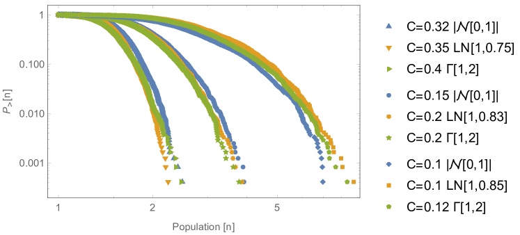
Figure 1: Cumulative RSA for a network of $9$ species, where matrix elements of both $M_{ij}$ and $L_{ij}$ have been drawn from three different probability distributions ($z_{h}\sim p_{h}(z)$, $M_{ij}\sim z_{h}$, $L_{ij}\sim z_{h}$, $L_{ji}\sim-z_{h}$, $h=1,2,3$): the modulus of a Normal distribution $z_{1}\sim|\mathcal{N}(\alpha,\beta)|$ (blue lines), Gamma distribution $z_{2}\sim\Gamma(\alpha,\beta)$ (green lines) and LogNormal distribution $z_{3}\sim LN(\alpha,\beta)$ (orange lines lines). Plots display averages over 100 realizations (assuming self-averaging this is equivalent to consider large $S$). Connectivity for mutalistic interaction ($M$) is denoted by $C_{M}=C$, while for exploitative interactions is $C_{L}=0.1C$ (in all the studied cases $C_{M}+C_{L}\leq 1$). $\epsilon_{1}=\epsilon_{2}=1$. We set the distribution parameters $\alpha,\beta$ (see legend) so that in each case we build interaction matrices with three different values of coefficient of variation $\text{CV}\approx 2,3,4$. As we can see, the cumulative RSA is not very sensible to the distribution from which the matrix elements of both $M_{ij}$ and $L_{ij}$ are drawn, but only on the CV. The analytical formula of $\mu_{M},\mu_{L},\sigma^{2}_{M},\sigma^{2}_{L}$, which depend the network size, connectivity and correlations are presented in the Methods section.

We define species abundance fluctuations as $x^{i}_{N}(t)=\sqrt{N}\left(\bar{\eta}^{i}(t)-m_{i}\right)$ for $i=1,\ldots,S$. Another relevant quantity characterizing the ecosystem biodiversity is the covariance matrix $V$, $V_{ij}=\langle x^{i}(t)x^{j}(t)\rangle-\langle x^{i}(t)\rangle\langle x^{j}(t)\rangle$, describing the correlations in the population abundance fluctuations between pairs of species population abundances [63]. In our setting we can compute analytically this quantity in the limit of normal fluctuations. The stochastic process $\left(x^{1}_{N}(t),\ldots,x^{S}_{N}(t)\right)$ converges in distribution to a Gaussian Markov process $X:=\left(X^{1}(t),\ldots,X^{S}(t)\right)$, which solves the stochastic differential equation $dX=AX\>dt+\Phi dB_{t}$, where $B_{t}$ is a $S$-dimensional Brownian motion, which corresponds to a $S$-dimensional Ornstein-Uhlenbeck process [12, 21]. The analytical expressions for the matrices $A$ and $\Phi$ in terms of the interaction matrices $M$ and $L$, and of the equilibria, $(m_{1},\dots,m_{S})$, of Eq. 17, are given in the Supporting Information, section 3. The covariance matrix, $V$, can be obtained by solving the following Lyapunov matrix equation $A\>V+V\>A^{T}+\Phi\Phi^{T}=0$.

This quantity is typically measured from species population time series, through the Pearson (or other type of) correlations [13]. Moreover, in many studies once opportunely thresholded, it is used as an empirical proxy of the species interactions matrix [13, 38]. In other words many works assume that $L+M$ can be approximated through $V$. Other works, applying maximum entropy approach, use $V^{-1}$ as the quantity to describe the species interactions network [63]. However we find that both $V$ and $V^{-1}$ are not good proxies of the species interactions matrix $M+L$ (see Supporting Information, section 4). This result highlights the importance to properly infer interaction networks from data [13, 16] by considering a suitable model, which explicitly takes into account species interactions.

2.3 The importance of cooperation: a solution of the stability-complexity paradox

We now show how our shift in the assumptions behind mutualistic/commensalistic species interactions could resolve the problematic aspect of stability in ecosystem dynamics. In particular, for $\epsilon_{1}=\epsilon$ and $\epsilon_{2}=0$ (voter model with cooperation and indirect competition, but no exploitation) we are able to analytically relate key dynamical features of Eq. 17 to the topology of the interaction matrix $M$ and prove various results of ecological importance.

First we show that the presence of non-supported species – the i-th species is non-supported if $\sum_{j}M_{ji}=0$ – inhibits coexistence equilibria of the whole ecological community. More precisely, if species $i$ is non-supported by other species then at stationarity Eq. 17 implies that $m_{i}=0$. The extinction of the $i$-th may create new unsupported species that go to zero in the large time limit. Such a cascade of extinctions may eventually end only when $\sum_{j}M_{ji}>0$ for all nodes/species $i$ of the network (see Supporting Information, section 4). The elimination of nodes of the interaction network corresponding to all non-supported species will be called pruning in the following.

Furthermore, we have found sufficient conditions on the topology of the mutualistic interaction matrix $M$ for the existence of stable stationary states of Eq. 17. In fact, if $M$ is irreducible, i.e. if for any node $i$ we can reach any other node $j$ through a path of oriented links $(k,l)$ such that $M_{kl}>0$, then the Perron-Frobenius (PF) theorem holds [52] and it exists a unique non-trivial stationary state $(m_{1},\dots,m_{S})$ with only positive entries. This solution is proportional to the left eigenvector, $v$, of $M$ corresponding to the eigenvalue of $M$ with the largest modulus, which turns out to be non-degenerate, real and positive [52], denoted by $\alpha$ in the following (and that for brevity we will refer to it as PF eigenvalue). In other word, if $M$ satisfies the PF theorem, then $\alpha$ tell us how the stationary species abundances $m$ are distributed. The corresponding right eigenvector will be denoted by $w$, and it gives information on how press perturbations spread throughout the network [57]. All components of both $v$ and $w$ are strictly positive and $m_{i}=v_{i}/\sum_{k}v_{k}$. An example of irreducible matrix $M$ occurs when $M_{ij}>0$ implies $M_{ji}>0$ and the network has a single connected component. Many networks architectures that have been observed in natural ecological communities satisfy this condition (e.g. hierarchical modular structure in mutualistic networks[5]).

Therefore, within our framework, we can analytically study the impact of the species interaction network architecture on system stability and species extinction. The results of the mean field predictions are shown in Fig. 2. Two simple examples are shown corresponding to an ecosystem with no extinction (panels A-B) and with extinction (panels C-D).

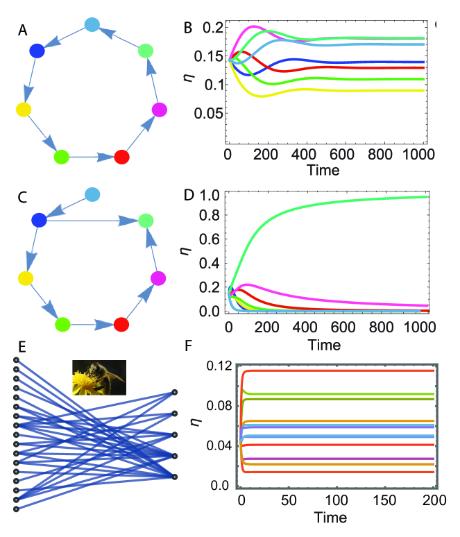
Figure 2: (A) Species interaction network for $7$ species where each species $i$ has one mutualistic partner $j$, i.e. $M_{ij}=1$, $\epsilon_{1}=1$, $\epsilon_{2}=0$. (B) Time evolution of the populations of the $7$ species as predicted by the mean field dynamics Eq. 17. (C) Species interaction network where one species is not helped by any species and the iterative pruning process, as described in the text, leads to a cascade of extinctions (D) as the time evolution of the mean field Eq. 17 shows, leading to only one species dominating the community. (E) Nested structure for fruit eating birds community in Mexico [33]. (F) All species coexist, as predicted by our theoretical framework. In the ordinate axis use the notation $\bar{\eta}$ and not $\eta$.

More generally, we can study analytically the stability of the equilibria as a function of ecological complexity, by analyzing the eigenvalues of the linearization of Eq. 17, i.e. the Jacobian matrix $A$, around the equilibria, $m_{i}$, of the system. We set equal to zero the diagonal of $M$ whereas the off-diagonal pair $(M_{ij},M_{ji})$ is equal to $(0,0)$ with probability $1-C$ and with probability $C$ it is drawn from a bivariate Gaussian distribution of means $(\mu,\mu)^{T}$ and interaction covariance matrix $\Sigma=(\sigma^{2},\rho\sigma^{2};\rho\sigma^{2},\sigma^{2})$. This guarantees that, for a connected cluster, coexistence of all species occurs. We define $\mu_{M}$, $\sigma_{M}^{2}$ and $\mu_{M}=C\mu,\ \sigma_{M}^{2}=C\sigma^{2}+C(1-C)\mu^{2},\ \rho_{M}=\frac{\rho\sigma^{2}+(1-C)\mu^{2}}{\sigma^{2}+(1-C)\mu^{2}}$ as mean, variance and correlation of the elements of matrix $M$. The case in which each element of $M_{ij}$ is assigned independently of $M_{ji}$ simply correspond to the case $\rho=0$ (notice that even if $\rho=0$ we can have $\rho_{M}\neq 0$). Similarly, when considering also exploitative interactions, we can sample randomly the off-diagonal pairs $(L_{ij},L_{ji})$, obtaining a given mean $\mu_{L}$, variance $\sigma_{L}^{2}$ and correlation $\rho_{L}$. If $\mu_{M}\geq\sigma_{M}\sqrt{(1+\rho_{M})/S}$, the leading eigenvalue $\lambda_{M}=S\mu_{M}=SC\mu$ and the corresponding eigenvector has positive components [1]. Moreover, the components of the leading eigenvector are approximately constant, i.e. the equilibria of system given by Eq. 17 can be written as $m_{i}=\frac{1}{S}(1+\xi_{i})$ for $i=1,\ldots,S$ with $\sum_{i}\xi_{i}=0$. Using the fact that $1=Sm_{i}-\xi_{i}$, $\lambda_{M}=S\mu_{M}$ and taking into account that all the terms involving $\xi_{j}$ are sub-leading in $S$, we obtain that the leading term of the system Jacobian does not depend on $L$ (see Methods) and it is equal to:

$$A_{ij}=-\delta_{ij}S\mu_{M}+\left(M_{ij}-\mu_{M}\right)=-\delta_{ij}S\mu_{M}+M^{\prime}_{ij}\ ,$$ (4)

where $M^{\prime}_{ij}:=M_{ij}-\mu_{M}$ is a random matrix with zero mean variance $\sigma_{M}^{2}$ and correlation $\rho_{M}$. This implies that the eigenvalues are uniformly distributed in an ellipse centered around $-S\mu_{M}$ with semi-axis $\sqrt{S}\sigma_{M}(1+\rho_{M})$ and $\sqrt{S}\sigma_{M}(1-\rho_{M})$ [22, 53]. The largest eigenvalue of the Jacobian is therefore given by $-S\mu_{M}+\sqrt{S}\sigma_{M}(1+\rho_{M})$. Thus, for fixed connectivity, $C$, in the presence of cooperation the system stability increases with $S$, whereas if only predator-prey interactions are present, then the stability decreases for increasing ecosystem complexity, as the May theorem would predict (Figure 3).

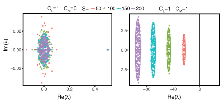
Figure 3: Eigenvalues ($\lambda$) spectrum of the Jacobian matrix $A$ around the stationary state for different size (colors) of the networks (from $S=50$ to $S=200$). The off-diagonal elements of matrices $M$ and $L$ are drawn uniformly between 0 and 1, i.e. $M_{ij}\sim z$, $L_{ij},L_{ji}\sim\pm z$, $z\sim U(0,1)$. Left panel: (A) Pure exploitative interactions ($C_{L}=1,\epsilon_{2}=1$,$\epsilon_{1}=0$); Right panel: (B) Exploitative and mutualistic interactions ($C_{L}=C_{M}=0.5,\epsilon_{1}=\epsilon_{2}=1$). The points are the eigenvalues of one Jacobian matrix obtained sampling at random the matrices M and L, while the lines indicate the analytical prediction for the support of the $A$ eigenvalues in the corresponding cases (see Eq. 4). The black vertical line indicates the instability threshold.

3 Discussion

Our results can be applied to study the effect of the interaction network topology to species coexistence in real mutualistic ecological communities. In particular, we found that nested architecture [6], observed in plant - pollinators ecological communities [5, 59], where specialist species, with only few mutualistic links, tend to interact with a proper subset of the many mutualistic partners of any of the generalist species, (see Fig. 2 panel E) satisfies the hypothesis of the PF theorem and thus favour species coexistence (Fig. 2 panel F).

We have also numerically explored the effect of adding exploitation, i.e. $\epsilon_{2}\neq 0$ and $C_{L}>0$ (see Fig. 4). Specifically we find that adding exploitations does not change the main conclusions of our results, as long as a mutualistic network of interactions is present, corresponding to an irreducible matrix, $M$, and the transition rates given by Eq. 1 never become negative during the time evolution of the mean field equation Eq. 17 (otherwise it would invalidate the derivation of the mean field equations themselves, see Methods section and Supporting Information, section 5).

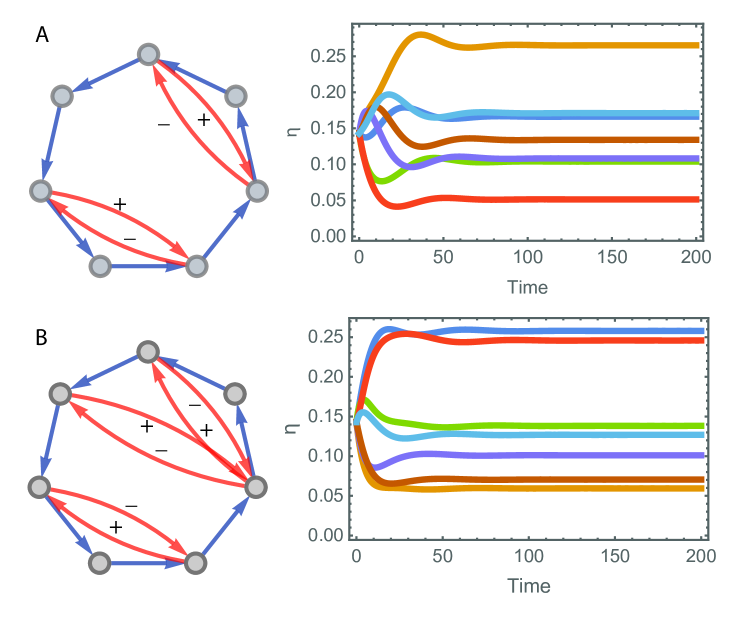
Figure 4: Species interaction network for $7$ species where each species $i$ has one mutualistic partner $j$, i.e. $M_{ij}=1$, and also two (A) and three (B) exploitative (+-) interactions ($\epsilon_{1}=\epsilon_{2}=1$). The corresponding time evolution of the populations of the $7$ species, as predicted by the mean field dynamics Eq. 17, are also shown. During the time evolution the rates given by Eq. 1 remain positive and extinctions are not observed.

We have shown that by properly deriving the contribution of mutualism in the species population dynamics, we solve two long standing problems in theoretical ecology: how a large number of species can coexist together and the complexity-stability paradox. In fact, we found that cooperation promotes ecosystem biodiversity, that in turn increases its stability without any fine tuning of the species interaction strengths or of the self-interactions [58]. Even moderate mutualistic interactions can stabilize the dynamics and if present the stability increases with the ecosystem complexity (see Fig. 3 and Fig. S5-S6 in the Supporting Information).

Our framework proposes an alternative approach to model cooperation in species population dynamics starting from an individual based stochastic model. We have developed a generalization of the classic voter model, adding the effect of species interactions on birth rates. We have shown that a shift in the assumptions behind mutualistic/commensalistic interactions resolve long-standing open theoretical question on the relation between stability and complexity and provides a unifying modeling approach useful to describe emergent patterns in ecology and interacting large ecological systems. We highlight that, when properly accounted in the dynamics, mutualistic/commensalistic relationship are crucial in order to have coexistence of species in the communities, as observed recently in real microbial communities [24, 46].

4 Method

4.1 Application of the Perron Frobenius Theorem to the Model Equations

Let us consider the dynamics given by Eq. (17) for $\epsilon_{2}=0$. If $M$ is irreducible, then the PF theorem holds [52] and given the initial condition $\bar{\eta}^{i}(0)>0\ i=1,\dots,\ S$, the time dependent solution for the species fractions is

$$\bar{\eta}(t)=\frac{\bar{\eta}(0)^{T}e^{\epsilon Mt}}{\sum_{i}(\bar{\eta}(0)^{T}e^{\epsilon Mt})_{i}}$$ (5)

Since for any eigenvalue, $\beta\neq\alpha$, of $M$ we have $\Re(\beta)<\alpha$ the dominant term in both numerator and denominator in Eq. 5 is $v\ e^{\alpha t}(\bar{\eta}(0)\cdot w)$ leading to $\lim_{t\to\infty}\bar{\eta}(t)=\frac{v}{\sum_{i}v_{i}}=m$. This is an easy computation when $M$ has a basis of eigenvectors and in general can be derived using the Jordan decomposition. As a corollary of the derivation above we have also that the stationary solution is globally stable in the region $\bar{\eta}^{i}(0)>0$, for all $i=1,\ldots,N$.

4.2 Analytical justification of the coexistence condition

As explained in the main text, if the matrix $M$ is irreducible and the transition rates given by Eq. 1 are positive during the time evolution (a necessary condition in order that the derivation of the mean field is justified), then we find numerically that, even in presence of a large concentrations of exploitative interactions, at stationarity the system still admits an high biodiversity and full coexistence is observed (see Fig. 4). Here we want to heuristically justify what we have observed numerically. Adding exploitative interactions does not lead to extinctions, as long as the mutualistic network of interactions is present, corresponding to an irreducible matrix, $M$. We argue that, under this hypothesis, when $\bar{\eta}^{s}$ is positive but close to zero the complete mean field equations - where both $\epsilon_{1}$ and $\epsilon_{2}$ are positive - are perturbation of the mean field equation where only mutualistic interaction are present, since we have proved that a pure mutualistic system has no extinction as long as the matrix $M$ is irreducible. Following the notation in Results, our continuous time Markov process is defined by the rule: a randomly chosen individual is removed and substituted by an individual of the $j$-th species at a rate

$$\omega(j,\eta,M,L)=\underbrace{\bar{\eta}^{j}+\epsilon_{1}\sum_{k}\bar{\eta}^{k}M_{kj}\theta(\bar{\eta}^{j})}_{:=\omega_{j}^{M}}+\underbrace{\epsilon_{2}\sum_{k}\bar{\eta}^{k}L_{kj}\bar{\eta}^{j}}_{:=\omega_{j}^{L}},$$ (6)

where $\epsilon_{1}>0$ and $\epsilon_{2}>0$ give the cooperation and exploitation intensity, and $\theta(\cdot)$ is the Heaviside step function, i.e., $\theta(x)>0$ when $x>0$ and 0 otherwise. As $N\to\infty$ the relative abundance $\bar{\eta}^{s}$ converges to the solution of the system of ordinary differential equation for $s=1,\ldots,S$. Equation for $\bar{\eta}^{s}$, when $\bar{\eta}^{s}$ is positive but close to zero, can be written in the following form

$$\dfrac{\mathrm{d}}{\mathrm{d}t}\bar{\eta}^{s}(t)=\underbrace{\omega^{M}_{s}-\bar{\eta}^{s}(t)\sum_{i}\omega^{M}_{i}}_{\simeq\delta>0}+\mathcal{O}(\bar{\eta}^{s})$$ (7)

The first two terms in Eq. 7 are the vector fields corresponding to mean field equation for $M$ irreducible and no exploitation (i.e. $\epsilon_{2}=0$). We know that such a system has no extinctions and its vector field is typically greater than $\delta>0$ out of equilibrium when $\bar{\eta}^{s}\simeq 0$. The last term in Eq. 7 contains terms which are linear dependent of $\omega_{j}^{L}$ which is $\mathcal{O}(\bar{\eta}_{s})$. Thus $\dfrac{\mathrm{d}}{\mathrm{d}t}\bar{\eta}^{s}(t)$ is positive for $\bar{\eta}^{s}$ close to zero. The requested transition rates never become negative during the time evolution of the mean field equation. This is a necessary condition otherwise the derivation itself of the mean filed equation would be meaningless.

4.3 Stability of the equilibria

In the case of $\epsilon_{2}\neq 0$, the entries of the Jacobian read

$$A_{ij} =\epsilon_{1}\left(M^{T}_{ij}-\delta_{ij}\sum_{h,k=1}^{S}m_{h}M_{hk}-m_{i}\sum_{k=1}^{S}M_{jk}\right)$$

$$+\epsilon_{2}\left(L_{ji}m_{i}+\delta_{ij}\sum_{k=1}^{S}m_{h}L_{hi}-\delta_{ij}\sum_{h,k=1}^{S}m_{h}L_{hk}m_{k}\right.$$

$$\left.-m_{i}\sum_{k=1}^{S}L_{jk}m_{k}-m_{i}\sum_{k=1}^{S}L_{kj}m_{k}\right)$$

The diagonal entries of the Jacobian are

$$A_{ii}=-\epsilon_{1}\sum_{h,k=1}^{S}m_{h}M_{hk}+\epsilon_{2}\sum_{h=1}^{S}m_{h}L_{hi}-\epsilon_{2}\sum_{h,k=1}^{S}m_{h}L_{hk}m_{k}$$ (8)

Since $m_{i}\sim 1/S$, it is simple to observe that the term proportional to $\epsilon_{1}$ is of order $S$ (plus sub-leading fluctuations). On the other hand, the leading order of the terms proportional to $\epsilon_{2}$, is of order $1$ and therefore always sub-leading if $\epsilon_{1}>0$. A similar argument applies to the off-diagonal elements. In that case, the terms proportional to $\epsilon_{1}$ are of order $1$, while the ones proportional to $\epsilon_{2}$ are of order $1/S$.

Similarly to what found in the case $\epsilon_{2}=0$, we have that the following relations hold: $\mu_{L}=C_{L}\mu,\;\sigma_{L}=\sqrt{C_{L}\left(\sigma^{2}+(1-C_{L})\mu^{2}\right)},\;\rho_{L}=\frac{\rho\sigma^{2}+(1-C_{L})\mu^{2}}{\sigma^{2}+(1-C_{L})\mu^{2}}$ where $\mu$ and $\sigma$ are the mean and the standard deviation of the distribution from which we draw the value for the exploitative interaction strengths. These expressions have been used together with $\mu_{M}$, $\sigma_{M}$ and $\rho_{M}$, when calculating the coefficient of variation. The above considerations indicate that the distribution of the eigenvalues of the Jacobian, Eq. 8, is the same as the $\epsilon_{2}=0$ case. Figures visualising these results are presented in the Supporting Information (section 6).

Supporting Information

Mechanistic interpretation of linear growth rates

The mutualistic dynamics introduced in the main text assumes that the benefit that a species receives from other species is independent of its own abundance. This assumption is radically different from the typical form of growth rates for exploitative (e.g. predator-prey) interactions, where some sort of mass-action law, typical of chemical reaction, is usually invoked [55]. Here we consider mutualism/commensalism as the presence of certain species is able to create an environment (e.g. by producing some public good or nutrient) or to release some substances (e.g. faecal pellets, metabolic waste), which favor the growth of some others species.

The state at time $t$ of the system is given by species concentration vector (i.e., average fraction of individuals for each species) $\bar{\eta}^{i}(t)$ with $i=1,\ldots,S$ and let $c$ be the concentration of a given resource used by the species $j$. This resource is provided, at a rate $s$, by certain species, $k$’s (e.g. through metabolic waste/secretion [24, 60, 46] or, in the case of plant/flowers, it represents the pollen produced by the $k$’s species) and related to their populations in a linear way, that is $s(t)=\sum_{k}\bar{\eta}^{k}(t)M_{kj}$. The kinetic of nutrient concentration is then [50, 60]

$$\frac{dc(t)}{dt}=\frac{1}{\tau_{R}}\left(s(t)-\bar{\eta}^{j}(t)r(c(t))\right)$$ (9)

where $r(c)$ is the consumption rate per individual whose specific form is irrelevant for the purpose of this example (e.g., one can consider the Monod function $r(c)=\alpha c/(K+c)$, with $\alpha$ and $K$ some suitable constants). The constant $\tau_{R}$ is the timescale of the dynamics of resources.

The contribution to the growth rate $\Delta\omega_{j}$ of the $j$-th species, due to this nutrient, is

$$\Delta\omega_{j}=\epsilon r(c)\bar{\eta}^{j}$$ (10)

where $\epsilon$ is a conversion factor measuring how the nutrient contributes to the biomass of the $j$-th species. If the nutrient concentration is in quasi-steady state [50], that is $dc(t)/dt=0$, which occurs if it relaxes much faster than populations (i.e. for small $\tau_{R}$), then, from the above equation, we get

$$r(c(t))=\frac{s(t)}{\bar{\eta}^{j}(t)}$$ (11)

leading to

$$\Delta\omega_{j}=\epsilon s=\epsilon\sum_{k}\bar{\eta}^{k}M_{kj}$$ (12)

If $\bar{\eta}^{j}>0$, then we have that the rate is linear in the population of the mutualistic partners. We again highlight that this form is radically different from the typical growth rates proposed in the literature, where some sort of mass-action law, typical of chemical reaction, is usually invoked [55]. The latter assumption is in fact only appropriate when we are assuming that the contribution to the population growth depend on the physical encounter between two species, as typically happens for exploitative (e.g. predator-prey) interactions.

Mean field analysis for the voter model with empty sites

If we turn off exploitation ($\epsilon_{2}=0$), the mean field equation without empty site ($\epsilon_{1}=\epsilon$) reads

$$\dfrac{\mathrm{d}}{\mathrm{d}t}\bar{\eta}^{s}=\epsilon\>\sum_{k=1}^{S}\bar{\eta}^{k}M_{ks}\>\theta(\bar{\eta}^{s})-\epsilon\>\bar{\eta}^{s}\sum_{i,j=1}^{S}\bar{\eta}^{i}M_{ij}\>\theta(\bar{\eta}^{j})$$ (13)

where $s=1,\ldots,S$ represents different species, $\bar{\eta}^{s}$ is the average fraction of individuals of the $s$-th species, $M$ is the interaction matrix whose non-zero entries define the network of ecological interactions, $\theta$ is the Heaviside step function ($\theta(x)=1(0)$ for $x>0(x\leq 0)$ ) and $\epsilon$ is the cooperation intensity (the average of the non-zero $M_{ij}$ is fixed to $1$). For simplicity, we have omitted time dependence of $\bar{\eta}$. An intuitive derivation is as follows. The key point is that for $N$ large the evolution of the quantity $\bar{\eta}^{s}$ becomes deterministic because the noise is canceled in the macroscopic regime and in the thermodynamics limit the relative abundance converges to its mean. Then, observe that the dynamics of the relative abundance in the infinitesimal time $dt$ is simple as it can only decrease by $1/N$ when a site of kind $s$ change type or can increase by $1/N$ when the new symbol of a certain site is $s$.

We now extend the model presented in the main text introducing the possibility for a site to be empty. In our setting empty sites do not interact with species. Thus the species rates remain unchanged after the introduction of empty sites. Thus the species rates are the same as before whereas non-empty sites become empty with rate $\lambda$. In the case $\epsilon=0$, the rate $\lambda$ has to be less than 1 otherwise empty sites will cover all the available space. The mean field equations become now:

$$\dfrac{\mathrm{d}}{\mathrm{d}t}\bar{\eta}^{s} =\bar{\eta}^{s}\bar{\eta}^{0}-\bar{\eta}^{s}\lambda+\epsilon\sum_{k=1}^{S}\bar{\eta}^{k}M_{ks}\theta(\bar{\eta}^{s})-\epsilon\bar{\eta}^{s}\sum_{i,j=1}^{S}\bar{\eta}^{i}M_{ij}\theta(\bar{\eta}^{j})$$ (14)

$$\dfrac{\mathrm{d}}{\mathrm{d}t}\bar{\eta}^{0} =(1-\bar{\eta}^{0})(\lambda-\bar{\eta}^{0})-\epsilon\bar{\eta}^{0}\sum_{i,j=1}^{S}\bar{\eta}^{i}M_{ij}\theta(\bar{\eta}^{j})$$ (15)

Let us analyze the stationary mean-field equations for $\epsilon<<1$. In this case the stable equilibrium for the empty sites is $\bar{\eta}^{0}=\lambda-\epsilon\>\frac{\lambda}{1-\lambda}\sum_{i,j=1}^{S}\bar{\eta}^{i}M_{ij}\>\theta(\bar{\eta}^{j})+O(\epsilon^{2})$. Substituting in the equations for $\bar{\eta}^{s}$, we obtain

$$\epsilon\sum_{k=1}^{S}\bar{\eta}^{k}M_{ks}\theta(\bar{\eta}^{s})-\epsilon\left(\frac{1}{1-\lambda}\right)\bar{\eta}^{s}\sum_{i,j=1}^{S}\bar{\eta}^{i}M_{ij}\theta(\bar{\eta}^{j})+O(\epsilon^{2})=0$$ (16)

where $s=1,\ldots,S$. After the change of variable $\bar{\eta}^{\prime}=(1-\lambda)\bar{\eta}$, the above (16) reduces to the same equation as one would get for $\lambda=0$, i.e. in absence of empty sites the mean field equation becomes:

$$\dfrac{\mathrm{d}}{\mathrm{d}t}\bar{\eta}^{s}(t)=\epsilon_{1}\sum_{k=1}^{S}\bar{\eta}^{k}(t)M_{ks}\theta(\bar{\eta}^{s}(t))+\epsilon_{2}\sum_{k=1}^{S}\bar{\eta}^{k}(t)L_{ks}\bar{\eta}^{s}(t)-\bar{\eta}^{s}(t)\sum_{i,k=1}^{S}\Big{(}\epsilon_{1}\bar{\eta}^{k}(t)M_{ki}\theta(\bar{\eta}^{i}(t))+\epsilon_{2}\bar{\eta}^{k}(t)L_{ki}\bar{\eta}^{i}(t)\Big{)}$$ (17)

for $s=1,\ldots,S$, where $\sum_{j=1}^{S}\bar{\eta}^{j}(t)=1$ and is conserved by the dynamics.

In other words, when $\epsilon$ is small, the introduction of empty sites leads to stationary abundances which are trivially rescaled with respect to the case in absence of empty sites, as a consequence of the reduction of the available space.

Covariance matrix and Species Interaction Networks

In this section, we consider the normal fluctuations around the deterministic limit of Eq. 17. This allows us to calculate the matrix $V$ describing the correlation between pairs of species population abundances [63]. As highlighted in the main text, this quantity, once opportunely thresholded, is used as an empirical proxy of the species interactions network [13, 18, 38]. Other works, applying maximum entropy approach, use $V^{-1}$ as the quantity to describe species interactions [63, 56]. The aim of this section is to test how well $V$ or $V^{-1}$ approximate the true interactions described by $M+L$ in our model.

For sake of simplicity, we assume that the limiting dynamics start at the equilibrium $m_{1},\ldots,m_{S}$ with $0<m_{i}<1$, $i=1,\ldots,S$. Thus, we define the fluctuation process as

$$x^{i}_{N}(t)=\sqrt{N}\left(\bar{\eta}^{i}_{N}(t)-m_{i}\right)\mbox{ for }i=1,\ldots,S.$$ (18)

One can apply standard techniques of convergence of generators to get weak convergence to the thermodynamic limiting evolution [12]. Indeed, the stochastic process $\left(x^{1}_{N}(t),\ldots,x^{S}_{N}(t)\right)$ converges in distribution to a Gaussian Markov process $X:=\left(X^{1}(t),\ldots,X^{S}(t)\right)$ which solves the stochastic differential equation

$$dX=\>AX\>dt+\Phi dB_{t}$$ (19)

where $B_{t}$ is a $S$-dimensional Brownian motion and

$$A_{ij} =\epsilon_{1}\left(M^{T}_{ij}-\delta_{ij}\sum_{h,k=1}^{S}m_{h}M_{hk}-m_{i}\sum_{k=1}^{S}M_{jk}\right)$$

$$+\epsilon_{2}\left(L_{ji}m_{i}+\delta_{ij}\sum_{h=1}^{S}m_{h}L_{hi}-\delta_{ij}\sum_{h,k=1}^{S}m_{h}L_{hk}m_{k}-m_{i}\sum_{k=1}^{S}L_{jk}m_{k}-m_{i}\sum_{k=1}^{S}L_{kj}m_{k}\right);$$

$$(\Phi\Phi^{T})_{ij} =-2\left(m_{i}m_{j}(1+\epsilon_{1}m_{i}\sum_{h,k=1}^{S}m_{k}M_{kh}+\epsilon_{2}\sum_{h,k=1}^{S}m_{k}L_{kh}m_{h})\right)(1-\delta_{ij})$$

$$+2(1-m_{i})\left(m_{i}+\epsilon_{1}\sum_{k=1}^{S}m_{k}M_{ki}+\epsilon_{2}\sum_{k=1}^{S}m_{k}L_{ki}m_{i}\right)\delta_{ij}$$

where $i,\ j=1,\ldots,S$ and $\delta_{ij}$ is the Kronecker delta.

From Eq. 19, it is then possible to derive the dynamics of the covariance matrix (see [20] for details):

$$V_{ij}(t)=\langle X^{i}(t)X^{j}(t)\rangle-\langle X^{i}(t)\rangle\langle X^{j}(t)\rangle$$ (20)

Therefore, we have

$$\frac{d\>V(t)}{dt}=\>A\>V(t)+\>V(t)\>A^{T}+\Phi\Phi^{T},$$ (21)

and at stationarity the covariance matrix, $V_{ij}=\lim_{t\to\infty}V_{ij}(t)$, resolves the following equation

$$\>A\>V+\>V\>A^{T}+\Phi\Phi^{T}=0.$$ (22)

Eq. 22 is a Lyapunov equation, so we could apply standard algorithms to solve it numerically [47].

We have determined $V$ from the solution of Eq. 22 and determined $V^{-1}$. If one assume that the population fluctuations around their means are gaussian distributed, then $V^{-1}$ represents the species interaction matrix [36, 63]. Indeed, within a maximum entropy approach, $V^{-1}$ is typically used to infer species interactions based on the available information of the system [56]. In our framework and as shown by Eq. 21 and Eq. 22, the relation between the interaction matrix $M+L$ and the matrix $V$ or $V^{-1}$ is highly non-linear. Moreover, because of the constraint, $\sum_{j}V_{ij}=0$, $V$ is not invertible, and thus in order to compute $V^{-1}$ we apply a pseudo-inverse scheme, i.e. we invert $V$ is the subspace of spanned by the eigenvectors corresponding to non-zero eigenvalues. As shown in Fig. 5, even for very simple structure of matrix $M$ and $L$, $V$ and $V^{-1}$ are not good proxies of the species interactions. The results are shown for the model without empty sites, but there is no qualitatively difference with the model including empty sites. This result highlights the importance to properly infer interaction networks from data.

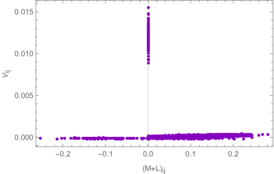
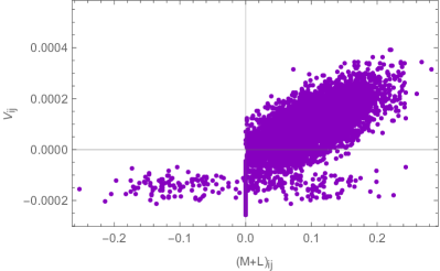
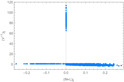
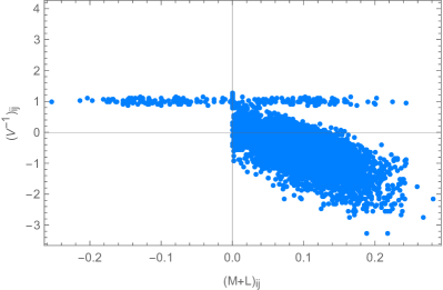
Figure 5: Elements of the covariance matrix $V$ and its inverse $V^{-1}$ compared to the species interaction network $M+L$ with size $S=100$, for dense mutualism $C_{M}=0.5$ and sparse exploitation $C_{L}=0.05$. Interaction strengths $z_{ij}$ have been drawn from a Gaussian distribution of mean $\mu_{N}=0.1$ and standard deviation $\sigma_{N}=0.05$. The sign has been then chosen accordingly ($M_{ij}=|z_{ij}|$; $L_{ij}=|z_{ij}|$ and $L_{ji}=-|z_{ji}|$). We have also imposed the irreducibility of $M$. Panels $(a),(c)$ represent the correlation over the whole of $L+M$ (between -0.3 and +0.3), while panels $(b),(d)$ zoom in the the relation close to the intersection of the $x$-$y$ axes. Although the zoom highlight a slightly positive (panel $b$) and negative (panel $d$) correlation between elements of $M+L$ and $V$, $V^{-1}$, they are not significant. Most of the elements of both the covariance matrix $V$ and its inverse $V^{-1}$ are close to zero. Other elements are very large, although the corresponding species do not interact (L+M=0), indicating that $V$ or $V^{-1}$ cannot be used as interaction matrix.

Topology of the Interaction Networks, Coexistence and Stationary States

In this section, we discuss some features of the topology of the mutualistic interaction matrix $M$ and how they relate to stationary states of the system. The main concept in this section is the one of pruned graph and the operation of pruning a network. A node with in-degree equals to zero and out-degree different from zero is called a dead leaf of the network. The operation of pruning consists in eliminating one by one the dead leaves of a given network together with their outbound links. After a first pruning, we will obtain a new network (that is a subnetwork of the starting one) that may still have dead leaves - the elimination of dead leaves may create new dead leaves. The pruning process end when the resulting network has no more dead leaves. The latter network is called stable or pruned. It is easy to see that the minimal pruned network (i.e. with the smallest number of links) that can be constructed with $S$ nodes is the cyclic graph. More in general, we have:

Proposition: The pruned network is a union of isolated nodes and graphs that contain at least one cycle each.

Indeed, pruning stops when the obtained graph is a union of isolated nodes and graphs where all nodes have at least an ancestor (i.e. the in-degree of each node is positive). Now a finite graph where each node has a least one incoming link contains at least a cycle. In fact, starting from one node it is possible to walk through the ancestors and never stop. Since the graph is finite, soon or later, the walker will visit twice the same node - so the walk contains a cycle - at most after a number of steps that equals the size of the graph.

The pruned network has at least one cycle but when not simply union of isolated cycles it can be very complex. Fig. 6 shows an example of the pruning procedure and of a non-trivial pruned network.

Figure 6: The diagram of how to prune network. (a) An example of how the operation of pruning works. First the 0-node is eliminated with its outbound link. After that, the node 1 becomes a dead leaf and has to be pruned. The cycle shown by the red links is the resulting pruned network. (b) An example of a pruned network that is not composed only by cycles.

As we anticipated at the beginning of this section, the dynamics of species sitting on dead leaves of the interaction network is trivial as their relative abundance goes to zero. This is a simple consequence of the fact that a dead leaf has no incoming bond. Thus, when $s$ is a dead leaf, the first term on the right of Eq. 13 is zero and simple estimate gives $\mathrm{d}\bar{\eta}^{s}/\mathrm{d}t=-\epsilon\>\bar{\eta}^{s}\sum_{i,j}\bar{\eta}^{i}M_{ij}\theta(\bar{\eta}^{j})\leq 0$. The previous simple remark leads to the following:

Limiting dynamics of dead leaves: Start the dynamics from a point with $\bar{\eta}^{i}\neq 0$ for all $i=1,\ldots,S$. If $k$ is a dead leaf then $\lim_{t\to\infty}\bar{\eta}^{k}(t)=0$.

Thus the presence of a dead leaf inhibits coexistence equilibria on the whole graph. More precisely, if $i=1,\ldots,\gamma$ are dead leaves (at some step of the pruning), the stable equilibria must have $\bar{\eta}^{1}=\ldots=\bar{\eta}^{\gamma}=0$.

Mean Field Equations, Birth Rates and Species Coexistence

We have numerically and systematically investigated the number of extinctions in ecological systems with both mutualistic and exploitative species interactions, as a function of different parameters: the average interaction strengths $\mu=\mu_{L}=\mu_{M}$, the connectance $C_{M}$, $C_{L}$, the network size $S$, etc. In all these cases we found that, as long as the birth rates (given by Eq. 1 in the main text) remain positive during the evolution, extinctions are not observed (see Fig. 7 and 8).

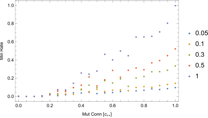
Figure 7: Plot of the Min Rate defined as $\min_{j=1,\dots,S,t\geq 0}\omega(j,\eta(t),M,L)$, where the rates $\omega$ are given by Eq. (1) in the main text and $\eta(t)$ is the mean field solution of Eq. 17, as a function of the connectivity of mutualistic $C_{M}=C_{++}$ and exploitative $C_{L}=1-C_{M}$ interactions for different average interaction strengths (colored points) $\mu=\mu_{M}=\mu_{L}=0.05,0.1,0.3,1$ (see legend) and $\epsilon_{1}=\epsilon_{2}=1$. In all cases the distribution from which interaction strengths are drawn as explained in main text from a bivariate Gaussian distribution with mean $\mu$ and standard deviation ($\sigma=0.01\mu$). The network size considered here is $S=20$. Similar results are found also for $S=50$ and $S=100$. The only cases where the birth rates (given by Eq. 1 in the main text) become negative during the mean field evolution, occur when exploitative interactions are dominant (region for $C_{M}<0.2$, $C_{L}>0.8$).

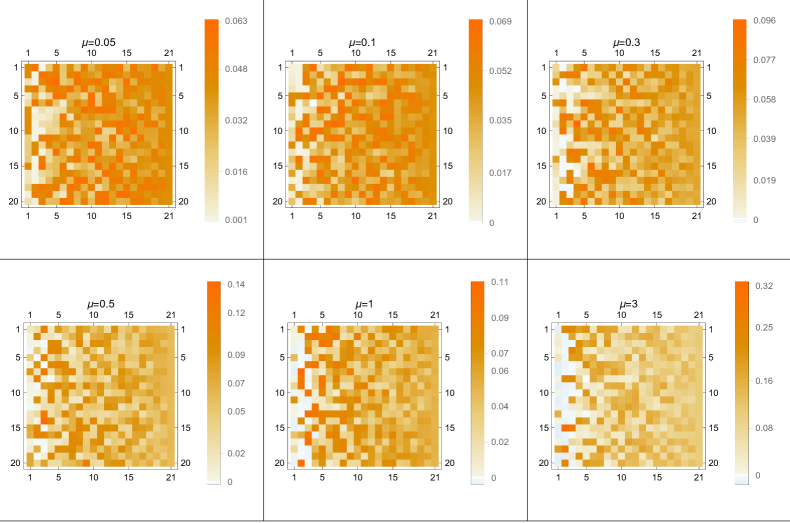
Figure 8: Populations of the species at the stationary state of the dynamics given by Eq. 17 and the same parameters set in Fig. 7. The $y$-axis denotes the species label (from $1$ to $20$), while the $21$ points in the $x$-axis represents the $21$ different connectivity configurations: from $C_{M}=0$ to $C_{M}=1$ with steps of $\Delta C_{M}=0.05$ and $C_{L}=1-C_{M}$. We numerically checked that as long as the birth rates (given by Eq. 1 in the main text) are positive, then no extinctions are observed (all species populations greater than zero).

Stability of the equilibria when $\epsilon_{2}\neq 0$

As shown in the Methods section of the main manuscript, the exploitative interactions do not contribute to the stability of the fixed point in the large $S$ limit if $\epsilon_{1}>0$ (see Fig. 9 and 10). Here we present numerical simulations visualizing this result.

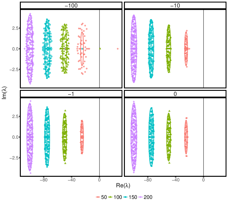
Figure 9: Spectrum of the Jacobian matrix. Different panels correspond to different values of $\epsilon_{2}=-100,-10,-1,0$ (as denoted at the top of each inset), while $\epsilon_{1}=1$ for all the simulations. The points are the eigenvalues of one Jacobian matrix obtained sampling at random the matrices $M$ and $L$, whose off-diagonal elements are both drawn uniformly between $0$ and $1$, while the lines indicate the analytical prediction obtained in the Methods section of the main text, in the case $\epsilon_{2}=0$. Colors and shapes correspond to different number of species ($S=50,100,150,200$ as denoted by the bottom legend). In all the cases, larger matrices turn out to be more stable. The black vertical line indicates the stability threshold.

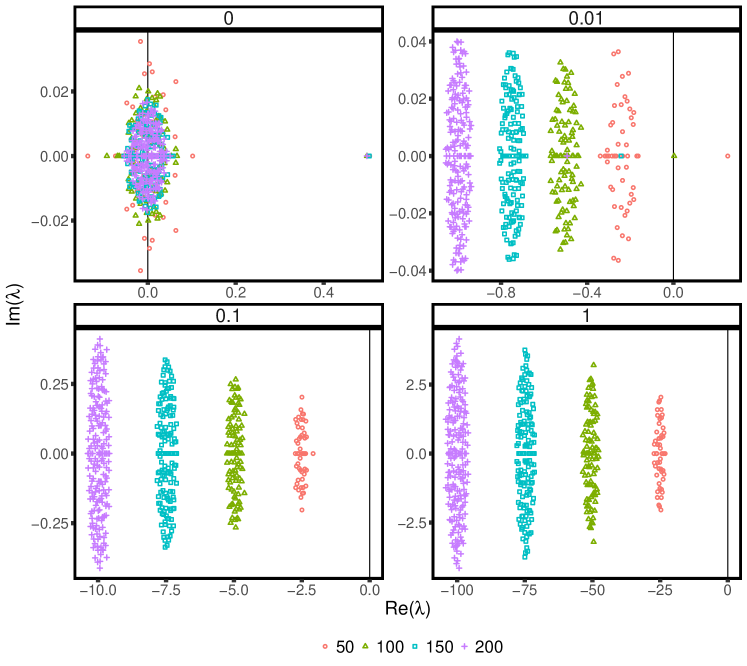
Figure 10: Same as in Fig. 9 but with $\epsilon_{2}=1$ and varying $\epsilon_{1}=0,0.01,0.1,1$ (as denoted at the top of each inset). Colors and shapes correspond to different number of species. When $\epsilon_{1}=0$, the system is always unstable. As soon as a $\epsilon_{1}>0$ is considered, the spectrum shift on the left, making the system stable. It is important to observe that this happens even for very small values of $\epsilon_{1}$. The minimum $\epsilon_{1}$ needed to stabilize the system is in fact expected to go to zero as the number of species $S$ increases ($S=50,100,150,200$ as denoted by the bottom legend). The off-diagonal elements of the matrices $M$ and $L$ are both drawn uniformly between $0$ and $1$.

Author contributions CT and SS contributed equally to this work. SS, MF and AM designed the study, CT, JG and SS performed numerical simulations, AM, MF and JG performed analytical calculations. All authors contributed in writing the manuscript.

Author declaration The authors declare that they have no competing financial interests.

Acknowledge We acknowledge enlightening discussions with Stefano Allesina, Sandro Azaele, Jayanth Banavar and Miguel Muñoz. S.S., C.T., A.M. acknowledge Fondazione Cariparo for financial support. S.S. acknowledge the Department of Physics and Astronomy, UNIPD for support to SID grant 2017 and the University of Padova for the STARS grant 2017. M.F. was partially supported by the INdAM – GNAMPA Project 2017 “Collective periodic behavior in interacting particle systems” and by Grant P201/12/2613 of the Czech Science Foundation (GACR).

References

- [1] Stefano Allesina and Si Tang. Stability criteria for complex ecosystems. Nature, 483(7388):205–208, 2012.
- [2] David Alonso, Rampal S Etienne, and Alan J McKane. The merits of neutral theory. Trends in ecology & evolution, 21(8):451–457, 2006.
- [3] Sandro Azaele, Samir Suweis, Jacopo Grilli, Igor Volkov, Jayanth R Banavar, and Amos Maritan. Statistical mechanics of ecological systems: Neutral theory and beyond. Reviews of Modern Physics, 88(3):035003, 2016.
- [4] György Barabás, Simone Pigolotti, Mats Gyllenberg, Ulf Dieckmann, and Géza Meszéna. Continuous coexistence or discrete species? a new review of an old question. 2012.
- [5] Jordi Bascompte and Pedro Jordano. Plant-animal mutualistic networks: the architecture of biodiversity. Annu. Rev. Ecol. Evol. Syst., 38:567–593, 2007.
- [6] Jordi Bascompte, Pedro Jordano, Carlos J Melián, and Jens M Olesen. The nested assembly of plant–animal mutualistic networks. Proceedings of the National Academy of Sciences, 100(16):9383–9387, 2003.
- [7] Enrico Bertuzzo, Samir Suweis, Lorenzo Mari, Amos Maritan, Ignacio Rodríguez-Iturbe, and Andrea Rinaldo. Spatial effects on species persistence and implications for biodiversity. Proceedings of the National Academy of Sciences, 108(11):4346–4351, 2011.
- [8] Claudio Castellano, Santo Fortunato, and Vittorio Loreto. Statistical physics of social dynamics. Reviews of modern physics, 81(2):591, 2009.
- [9] George WA Constable and Alan J McKane. Models of genetic drift as limiting forms of the lotka-volterra competition model. Physical review letters, 114(3):038101, 2015.
- [10] Katharine Z Coyte, Jonas Schluter, and Kevin R Foster. The ecology of the microbiome: networks, competition, and stability. Science, 350(6261):663–666, 2015.
- [11] Rick Durrett. Stochastic spatial models. SIAM review, 41(4):677–718, 1999.
- [12] Stewart N Ethier and Thomas G Kurtz. Markov processes: characterization and convergence, volume 282. John Wiley & Sons, 2009.
- [13] Karoline Faust and Jeroen Raes. Microbial interactions: from networks to models. Nature Reviews Microbiology, 10(8):538, 2012.
- [14] Charles K Fisher and Pankaj Mehta. The transition between the niche and neutral regimes in ecology. Proceedings of the National Academy of Sciences, 111(36):13111–13116, 2014.
- [15] Hugo Fort. Statistical mechanics ideas and techniques applied to selected problems in ecology. Entropy, 15(12):5237–5276, 2013.
- [16] Hugo Fort and Muhittin Mungan. Predicting abundances of plants and pollinators using a simple compartmental mutualistic model. In Proc. R. Soc. B, volume 282, page 20150592. The Royal Society, 2015.
- [17] Kevin R Foster and Thomas Bell. Competition, not cooperation, dominates interactions among culturable microbial species. Current biology, 22(19):1845–1850, 2012.
- [18] Jonathan Friedman and Eric J Alm. Inferring correlation networks from genomic survey data. PLoS Comput Biol, 8(9):e1002687, 2012.
- [19] Javier García-Algarra, Javier Galeano, Juan Manuel Pastor, José María Iriondo, and José J Ramasco. Rethinking the logistic approach for population dynamics of mutualistic interactions. Journal of theoretical biology, 363:332–343, 2014.
- [20] Crispin W Gardiner. Stochastic methods. Springer-Verlag, Berlin–Heidelberg–New York–Tokyo, 1985.
- [21] Crispin W Gardiner. Handbook of stochastic methods for physics, chemistry and the natural sciences, vol. 13 of springer series in synergetics, 2004.
- [22] Vyacheslav L Girko. The elliptic law. Teoriya Veroyatnostei i ee Primeneniya, 30(4):640–651, 1985.
- [23] BS Goh and LS Jennings. Feasibility and stability in randomly assembled lotka-volterra models. Ecological Modelling, 3(1):63–71, 1977.
- [24] Joshua E Goldford, Nanxi Lu, Djordje Bajic, Sylvie Estrela, Mikhail Tikhonov, Alicia Sanchez-Gorostiaga, Daniel Segre, Pankaj Mehta, and Alvaro Sanchez. Emergent simplicity in microbial community assembly. bioRxiv, page 205831, 2017.
- [25] Jacopo Grilli, Matteo Adorisio, Samir Suweis, György Barabás, Jayanth R Banavar, Stefano Allesina, and Amos Maritan. Feasibility and coexistence of large ecological communities. Nature communications, 8:0, 2017.
- [26] Jacopo Grilli, György Barabás, Matthew J Michalska-Smith, and Stefano Allesina. Higher-order interactions stabilize dynamics in competitive network models. Nature, 548(7666):210, 2017.
- [27] Alan Hastings. Food web theory and stability. Ecology, pages 1665–1668, 1988.
- [28] Crawford S Holling. Some characteristics of simple types of predation and parasitism. The Canadian Entomologist, 91(7):385–398, 1959.
- [29] Bahram Houchmandzadeh. Neutral aggregation in finite-length genotype space. Physical Review E, 95(1):012402, 2017.
- [30] S Hubbell. The Unified Theory of Biodiversity and Biogeography. Princeton Univeristy Press, 2001.
- [31] Pincelli M Hull, Simon AF Darroch, and Douglas H Erwin. Rarity in mass extinctions and the future of ecosystems. Nature, 528(7582):345, 2015.
- [32] G Evelyn Hutchinson. The paradox of the plankton. The American Naturalist, 95(882):137–145, 1961.
- [33] Gail E Kantak. Observations on some fruit-eating birds in mexico. The Auk, 96(1):183–186, 1979.
- [34] Simon A Levin. Public goods in relation to competition, cooperation, and spite. Proceedings of the National Academy of Sciences, 111(Supplement 3):10838–10845, 2014.
- [35] Jonathan M Levine, Jordi Bascompte, Peter B Adler, and Stefano Allesina. Beyond pairwise mechanisms of species coexistence in complex communities. Nature, 546(7656):56, 2017.
- [36] Timothy R Lezon, Jayanth R Banavar, Marek Cieplak, Amos Maritan, and Nina V Fedoroff. Using the principle of entropy maximization to infer genetic interaction networks from gene expression patterns. Proceedings of the National Academy of Sciences, 103(50):19033–19038, 2006.
- [37] Thomas M Liggett. Stochastic interacting systems: contact, voter and exclusion processes, volume 324. springer science & Business Media, 2013.
- [38] Gipsi Lima-Mendez, Karoline Faust, Nicolas Henry, Johan Decelle, Sébastien Colin, Fabrizio Carcillo, Samuel Chaffron, J Cesar Ignacio-Espinosa, Simon Roux, Flora Vincent, et al. Determinants of community structure in the global plankton interactome. Science, 348(6237):1262073, 2015.
- [39] Alfred J Lotka. Elements of physical biology. Williams and Wilkins Company, 1925.
- [40] Hirotsugu Matsuda, Naofumi Ogita, Akira Sasaki, and Kazunori Satō. Statistical mechanics of population: the lattice lotka-volterra model. Progress of theoretical Physics, 88(6):1035–1049, 1992.
- [41] Robert M May. Will a large complex system be stable? Nature, 238(5364):413, 1972.
- [42] Kevin McCann, Alan Hastings, and Gary R Huxel. Weak trophic interactions and the balance of nature. Nature, 395(6704):794, 1998.
- [43] Kevin Shear McCann. The diversity–stability debate. Nature, 405(6783):228–233, 2000.
- [44] Alan J McKane and Timothy J Newman. Stochastic models in population biology and their deterministic analogs. Physical Review E, 70(4):041902, 2004.
- [45] Brandon EL Morris, Ruth Henneberger, Harald Huber, and Christine Moissl-Eichinger. Microbial syntrophy: interaction for the common good. FEMS Microbiology Reviews, 37(3):384–406, 2013.
- [46] Alan R Pacheco, Mauricio Moel, and Daniel Segre. Costless metabolic secretions as drivers of interspecies interactions in microbial ecosystems. bioRxiv, page 300046, 2018.
- [47] Thilo Penzl. Numerical solution of generalized lyapunov equations. Advances in Computational Mathematics, 8(1):33–48, 1998.
- [48] Simone Pigolotti and Massimo Cencini. Speciation-rate dependence in species–area relationships. Journal of theoretical biology, 260(1):83–89, 2009.
- [49] Oscar A Pinto and Miguel A Munoz. Quasi-neutral theory of epidemic outbreaks. PloS one, 6(7):e21946, 2011.
- [50] Anna Posfai, Thibaud Taillefumier, and Ned S Wingreen. Metabolic trade-offs promote diversity in a model ecosystem. Physical review letters, 118(2):028103, 2017.
- [51] Angel M Segura, Danilo Calliari, Carla Kruk, Daniel Conde, Sylvia Bonilla, and Hugo Fort. Emergent neutrality drives phytoplankton species coexistence. Proceedings of the Royal Society of London B: Biological Sciences, page rspb20102464, 2010.
- [52] Eugene Seneta. Non-negative matrices and Markov chains. Springer Science & Business Media, 2006.
- [53] HJ Sommers, A Crisanti, Haim Sompolinsky, and Y Stein. Spectrum of large random asymmetric matrices. Physical review letters, 60(19):1895, 1988.
- [54] Vishal Sood and Sidney Redner. Voter model on heterogeneous graphs. Physical review letters, 94(17):178701, 2005.
- [55] Phillip PA Staniczenko, Jason C Kopp, and Stefano Allesina. The ghost of nestedness in ecological networks. Nature communications, 4:1391, 2013.
- [56] Richard R Stein, Debora S Marks, and Chris Sander. Inferring pairwise interactions from biological data using maximum-entropy probability models. PLoS Comput Biol, 11(7):e1004182, 2015.
- [57] Samir Suweis, Jacopo Grilli, Jayanth R Banavar, Stefano Allesina, and Amos Maritan. Effect of localization on the stability of mutualistic ecological networks. Nature communications, 6, 2015.
- [58] Samir Suweis, Jacopo Grilli, and Amos Maritan. Disentangling the effect of hybrid interactions and of the constant effort hypothesis on ecological community stability. Oikos, 123(5):525–532, 2014.
- [59] Samir Suweis, Filippo Simini, Jayanth R Banavar, and Amos Maritan. Emergence of structural and dynamical properties of ecological mutualistic networks. Nature, 500(7463):449–452, 2013.
- [60] Thibaud Taillefumier, Anna Posfai, Yigal Meir, and Ned S Wingreen. Microbial consortia at steady supply. eLife, 6:e22644, 2017.
- [61] M Vallade and B Houchmandzadeh. Analytical solution of a neutral model of biodiversity. Physical Review E, 68(6):061902, 2003.
- [62] Igor Volkov, Jayanth R Banavar, Stephen P Hubbell, and Amos Maritan. Neutral theory and relative species abundance in ecology. Nature, 424(6952):1035, 2003.
- [63] Igor Volkov, Jayanth R Banavar, Stephen P Hubbell, and Amos Maritan. Inferring species interactions in tropical forests. Proceedings of the National Academy of Sciences, 106(33):13854–13859, 2009.
- [64] Vito Volterra. Fluctuations in the abundance of a species considered mathematically. Nature, 118(2972):558–560, 1926.
- [65] Ned S Wingreen and Simon A Levin. Cooperation among microorganisms. PLoS biology, 4(9):e299, 2006.
- [66] Aleksej Zelezniak, Sergej Andrejev, Olga Ponomarova, Daniel R Mende, Peer Bork, and Kiran Raosaheb Patil. Metabolic dependencies drive species co-occurrence in diverse microbial communities. Proceedings of the National Academy of Sciences, 112(20):6449–6454, 2015.