Unseen Progenitors of Luminous High-$z$ Quasars in the $R_{\rm h}=ct$ Universe

Abstract

Quasars at high redshift provide direct information on the mass growth of supermassive black holes and, in turn, yield important clues about how the Universe evolved since the first (Pop III) stars started forming. Yet even basic questions regarding the seeds of these objects and their growth mechanism remain unanswered. The anticipated launch of eROSITA and ATHENA is expected to facilitate observations of high-redshift quasars needed to resolve these issues. In this paper, we compare accretion-based supermassive black hole growth in the concordance $\Lambda$CDM model with that in the alternative Friedmann-Robertson Walker cosmology known as the $R_{\rm h}=ct$ universe. Previous work has shown that the timeline predicted by the latter can account for the origin and growth of the $\gtrsim 10^{9}\;M_{\odot}$ highest redshift quasars better than that of the standard model. Here, we significantly advance this comparison by determining the soft X-ray flux that would be observed for Eddington-limited accretion growth as a function of redshift in both cosmologies. Our results indicate that a clear difference emerges between the two in terms of the number of detectable quasars at redshift $z\gtrsim 7$, raising the expectation that the next decade will provide the observational data needed to discriminate between these two models based on the number of detected high-redshift quasar progenitors. For example, while the upcoming ATHENA mission is expected to detect $\sim 0.16$ (i.e., essentially zero) quasars at $z\sim 7$ in $R_{\rm h}=ct$, it should detect $\sim 160$ in $\Lambda$CDM—a quantitatively compelling difference.

1 Introduction

The ongoing detection of quasars at high ($z\gtrsim 5$) redshift provides vital information regarding the growth of black hole (BH) mass and, in turn, informs our understanding of how the Universe has evolved since the beginning of the stelliferous era. To be sure, the assembly of the high-$z$ quasar sample has been painstaking work as these objects have proven to be quite elusive. As an example, Weigel et al. (2015) estimated that a search for $z\gtrsim 5$ AGNs in the Chandra Deep Field South (0.03 deg² field of view) should have lead to a discovery of $\sim 20$ AGNs, yet no convincing identifications were made. Such non-detections, while consistent with the seeming strong evolution at the faint-end of the AGN luminosity function with increasing redshift from $z\sim 3$ to $z\sim 5$ (Georgakakis et al. 2015), do put existing models of early black hole evolution at odds with observational constraints on their growth rate (Treister et al. 2013). Several possible explanations have been proposed for the very limited number of detections, including dust obscuration (Fiore et al. 2009), low BH occupation fraction, super-Eddington accretion episodes with low duty cycles (Madua et al. 2014; Volonteri & Silk 2015), and BH merging scenarios.

At the same time, the handful of $z>6.5$ quasars that have been observed (e.g., Mortlock et al. 2011) provide super-massive black hole (SMBH) mass estimates that are hard to reconcile with the timeline of a $\Lambda$CDM Universe (Melia 2013; Melia & McClintock 2015). Specifically, black holes in the local Universe are produced via supernova explosions with masses $\approx 5-20\;M_{\odot}$. But Eddington-limited accretion would require $\sim 10^{5}\;M_{\odot}$ seeds in order to produce the billion solar-mass quasars seen at redshift $z\gtrsim 6.5$. Accretion scenarios operating within the $\Lambda$CDM paradigm thus require either anomalously high accretion rates (Volonteri & Rees 2005) or the creation of massive seeds (Yoo & Miralda-Escudeé 2014), neither of which has actually ever been observed.

In recent work, Melia (2013) and Melia & McClintock (2017) present a simple and elegant solution to the supermassive black hole anomaly by viewing the evolution of SMBHs through the age-redshift relation predicted by the $R_{\rm h}=ct$ universe, a Friedmann-Robertson-Walker (FRW) cosmology with zero active mass. In their scenario, cosmic re-ionization lasted from $t\approx 883$ Myr ($z\sim 15$) to $t\approx 2$ Gyr ($z\sim 6$) (see also Melia & Fatuzzo 2016). As such, $5-20\;M_{\odot}$ black hole seeds that formed shortly after the beginning of re-ionization would have evolved into $\sim 10^{10}\;M_{\odot}$ quasars by $z\sim 6-7$ via the standard Eddington-limited accretion rate. It should be noted that these SMBH results are but one of many comparative tests completed between the $R_{\rm h}=ct$ and $\Lambda$CDM paradigms, the results of which show that the data tend to favor the former over the latter with a likelihood $\sim 90\%$ versus $\sim 10\%$, according to the Akaike (AIC) and Bayesian (BIC) Information Criteria (see, e.g., Wei et al. 2013; Melia & Maier 2013; Melia 2014; Wei et al. 2014a, 2014b; Wei et al. 2015a, 2015b; Melia et al. 2015). A summary of 18 such tests may be found in Table I of Melia (2017).

Clearly, our understanding of SMBH evolution remains an open question, with even the basic questions on how these objects were seeded and the mechanism through which they evolved remaining unanswered. But the next decade promises to be transformative. The eROSITA mission, scheduled for launch in 2018, will perform the first imaging all-sky survey in the medium energy X-ray range with unprecedented spectral and angular resolution. Likewise, the ATHENA X-ray observatory mission scheduled for launch in 2028 is expected to perform a complete census of black hole growth in the Universe tracing to the earliest cosmic epochs.

Motivated by the feasibility of testing the $R_{\rm h}=ct$ and $\Lambda$CDM paradigms with this upcoming wealth of observational data, we here extend the analysis of Melia (2013) and Melia & McClintock (2017) by using accretion-based evolutionary models of SMBHs to determine the expected soft X-ray flux values observable at earth as a function of redshift. The analysis is carried out for both Planck $\Lambda$CDM, with optimized parameters $\Omega_{\rm b}=0.308$, $w=-1$ and $H_{0}=67.8$ km s^-1 Mpc^-1, and the $R_{\rm h}=ct$ universe with the same Hubble constant for ease of comparison. We shall demonstrate that the quasar mass function for SMBHs at $z\gtrsim 7$ is considerably different between the two scenarios, indicating that the next generation of quasar observations at high-redshifts will allow us to discriminate between these two cosmologies.

The paper is organized as follows. We present our SMBH mass evolutionary model in §2, and relate it to redshift evolution in both $\Lambda$CDM and $R_{\rm h}=ct$. We then present our emission model in §3, which links the mass of a black hole to its X-ray emissivity. In §4, we combine the results of §2 and §3 to calculate the flux expected as a function of redshift during the evolutionary history of a SMBH for both the $\Lambda$CDM and $R_{\rm h}=ct$ cosmologies. These results are then combined with the known quasar mass function at $z=6$ in order to calculate the expected number of observable quasars as a function of redshift, again for both cosmologies. Our summary and conclusions are presented in §5.

2 Steady Eddington-limited Black-Hole Evolution in the Early Universe

We adopt a streamlined model wherein the early Universe ($6\lesssim z\lesssim 10$) is comprised of non-rotating black holes of mass $M_{\rm bh}$ that grow continuously through mass accretion via a thin or slim disk (see below), maintaining a constant radiative efficiency $\epsilon_{r}$ over that time (see, e.g., Chan et al. 2009). The ensuing bolometric luminosity is parametrized in terms of the Eddington ratio $\lambda_{\rm Edd}\equiv L_{bol}/L_{\rm Edd}$, which is also assumed to remain constant throughout this time. The disk accretion rate is therefore given by $\dot{M}=L_{bol}/(\epsilon_{r}c^{2})$, and with the further assumption that a black hole steadily accretes a fraction $(1-\epsilon_{r})$ of the infalling material (see, e.g., Ruffert & Melia 1994), the mass growth rate is

$$\dot{M}_{\rm bh}={(1-\epsilon_{r})\over\epsilon_{r}}{\lambda_{\rm Edd}L_{\rm Edd}\over c^{2}}={(1-\epsilon_{r})\over\epsilon_{r}}{\lambda_{\rm Edd}\over t_{\rm Edd}}\,M_{\rm bh}\,,$$ (1)

where $t_{\rm Edd}=0.45$ Gyrs. Integrating Equation (1), one obtains an expression for the black hole mass as a function of the age of the Universe,

$$M_{\rm bh}(t)=M_{0}\,e^{{(1-\epsilon_{r})\over\epsilon_{r}}{\lambda_{\rm Edd}\over t_{\rm Edd}}(t-t_{0})}\,,$$ (2)

where $M_{0}$ is the mass observed at redshift $z_{0}$, corresponding to an age $t_{0}$.

Connecting Equation (2) to observational cosmology requires a relation between redshift and the age of the Universe. In $\Lambda$CDM, this relation is given via the well known integral expression

$$t^{\Lambda}(z)={1\over H_{0}}\int_{z}^{\infty}{du\over\sqrt{\Omega_{m}(1+u)^{5}+\Omega_{\Lambda}(1+u)^{5+3w}}}\;,$$ (3)

where the radiation contribution has been omitted given the redshift of interest, thus leaving $\Omega_{\Lambda}=1-\Omega_{m}$. The corresponding expression for $R_{\rm h}=ct$ takes on the simpler form

$$t^{R_{\rm h}}(z)={1\over H_{0}(1+z)}\;.$$ (4)

We adopt the Planck parameters (Ade et al. 2016), $H_{0}=67.8$ km s^-1 Mpc^-1, $\Omega_{m}=0.308$, and $w=-1$, throughout this work.

The difference in age between $z\sim 10$ and $z\sim 6$ for the two scenarios, as illustrated in figure 1, has important implications for quasar evolution and detectability, and can therefore be used to test each model against present and future observations. Specifically, while the age of the Universe at $z=6$ is approximately $0.93$ Gyrs in standard ($\Lambda$CDM) cosmology, its value is approximately 2.1 Gyrs for $R_{\rm h}=ct$. As a result, a supermassive black hole in the $R_{\rm h}=ct$ universe has $\sim 18t_{\rm Edd}$ of additional time to grow before redshift $z=6$, and is therefore advantaged by a factor $\sim e^{18}\approx 6\times 10^{7}$ over its $\Lambda$CDM counterpart (assuming $\epsilon_{r}=0.1$ and $\lambda_{\rm Edd}=1$). More relevant to our discussion, the time interval between $z=6$ and $z=10$ in the $R_{\rm h}=ct$ universe is approximately $0.74$ Gyrs versus $0.46$ Gyrs in $\Lambda$CDM. As shown in figure 2, mass growth during this epoch in $R_{\rm h}=ct$ is therefore advantaged by a factor of $\sim e^{6}\approx 400$ over its $\Lambda$CDM counterpart for this scenario. These dramatically different growths, as measured by redshift, have important consequences on our ability to detect quasars at $z\gtrsim 7$, and is the primary focus of our work.

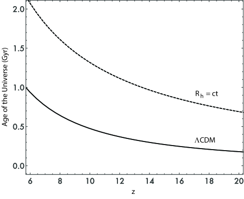
Figure 1: Age of the Universe versus redshift in both Planck $\Lambda$CDM (solid curve) and $R_{\rm h}=ct$, assuming the same Hubble constant for simplicity (dashed curve).

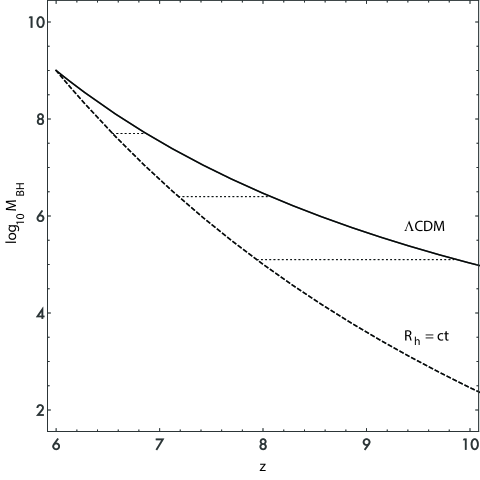
Figure 2: The mass evolution of a black hole with an observed mass $M_{0}=10^{9}\;M_{\odot}$ at redshift $z_{0}=6$ in both $\Lambda$CDM (solid curve) and $R_{\rm h}=ct$ (dashed curve), for the benchmark values $\epsilon_{r}=0.1$ and $\lambda_{\rm Edd}=1$. The thin dashed lines denote where the Universe was $1/3\,t_{\rm Edd}$, $2/3\,t_{\rm Edd}$ and $1\,t_{\rm Edd}$ younger than its age at $z=6$ which, for the adopted values of $\epsilon_{r}=0.1$ and $\lambda_{\rm Edd}=1$, correspond to a 3, 6 and 9 e-folding drop in mass.

3 Emission Model

3.1 Disk Emission

Our emission model follows the basic development in Pezzulli et al. (2017). In the classical model, a geometrically thin disk has an inner radius given by the last stable orbit at radius

$$r_{0}=3R_{\rm S}={6\,GM_{\rm bh}\over c^{2}}\,,$$ (5)

and has the temperature profile

$$T(r)=\left({3GM_{\rm bh}\dot{M}\over 8\pi\sigma r^{3}}\right)^{1/4}\,\left(1-\sqrt{{r_{0}\over r}}\right)^{1/4}\,,$$ (6)

for which the maximum temperature is achieved at $r={49\over 36}r_{0}$ (Shakura & Sunyaev 1973). If the disk emits a perfect blackbody, the bolometric luminosity is then given by the well know expression

$$L_{bol}={1\over 12}\dot{M}c^{2}\,,$$ (7)

which sets the radiative efficiency at $\epsilon_{r}=1/12$. One thus need only specify the black hole mass and the bolometric luminosity (or alternatively, the mass accretion rate $\dot{M}$) in order to calculate the emission from the disk.

To allow for a more general treatment where both $L_{bol}$ and $\epsilon_{r}$ can be used as model parameters, we calculate the disk emission through the expression

$$L_{\nu}=L_{0}\int_{r_{i}}^{\infty}B_{\nu}(T[r])\,r\;dr\,,$$ (8)

where $B_{\nu}$ is the Planck function and $L_{0}$ is a normalizing factor used to set the bolometric luminosity

$$L_{bol}=\int_{0}^{\infty}L_{\nu}\;d\nu\,.$$ (9)

The inner disk radius $r_{i}$ is determined by considering whether a thin disk or a slim disk serves as a better representation of the system under consideration (Abramowicz et al. 1988). Specifically, for a disk to remain geometrically thin, $L_{bol}\lesssim 0.3\,L_{\rm Edd}$. If this condition is not met, radiation pressure inflates the disk, which is then better described by a slim disk model. In this case, photons are trapped for radii $r\lesssim r_{pt}=1.5H(R_{\rm S}/r)(\dot{M}/\dot{M}_{\rm Edd})$, where $H$ is the half-disk thickness. Assuming $H/r=2/3$, and since $\dot{M}/\dot{M}_{\rm Edd}=L_{bol}/L_{\rm Edd}$, we therefore set $r_{i}=\hbox{Max}[3R_{\rm S},\lambda_{\rm Edd}R_{\rm S}]$.

3.2 Soft X-ray emission

X-ray surveys have proven to be suitable for identifying quasars at high redshift, and are advantaged over lower wavelengths due to a smaller amount of obscuration and less contamination or dilution from the host galaxy. The X-ray emission originates from a hot corona that surrounds the disk (see also Liu & Melia 2001), and can be parametrized as a power-law with exponential cutoff at $E_{c}=300$ keV:

$$L_{X,\nu}\propto\nu^{-\Gamma+1}e^{-h\nu/E_{c}}\,,$$ (10)

where the photon index is set through the empirical relation

$$\Gamma=0.32\log_{10}\left({L_{bol}\over L_{\rm Edd}}\right)+2.27\,,$$ (11)

(Brightman et al. 2013). We use the results of Lusso & Risaliti (2106; fig. 6) to then normalize the X-ray luminosity via the expression

$$\log_{10}L_{2\;{\rm keV}}=0.638\log_{10}L_{2500}+7.074\,,$$ (12)

where both luminosity densities are in units of erg s^-1 Hz^-1. The disk (solid) and X-ray (dashed) emission for systems with $M_{\rm bh}=10^{6}\;M_{\odot}$ and $10^{9}\;M_{\odot}$, both with $\lambda_{\rm Edd}=1$ and with $\epsilon_{r}=0.1$, are shown in figure 3.

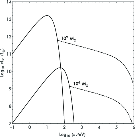
Figure 3: Emission from the disk (solid curve) and hot corona (dashed) of black holes with masses of $10^{6}$ and $10^{9}\;M_{\odot}$.

Since the greatest sensitivity to the emission produced in our model occurs in soft X-rays (see, e.g., Pezzulli et al. 2017), we consider only the soft X-ray band between $\epsilon_{l}=0.5$ keV and $\epsilon_{u}=2$ keV. For a black hole at redshift $z$, the luminosity emitted in this band is given by the expression

$$L_{X}=\int_{\epsilon_{l}(1+z)}^{\epsilon_{u}(1+z)}L_{X,\nu}\;d\nu\,.$$ (13)

The flux received at Earth is then given by

$$F_{X}={L_{X}\over 4\pi D_{L}^{2}}\,,$$ (14)

where $D_{L}$ is the luminosity distance, which in $\Lambda$CDM and $R_{\rm h}=ct$ are given, respectively, by the expressions

$$D^{\Lambda{\rm CDM}}={c\over H_{0}}(1+z)\int_{0}^{z}{du\over\sqrt{\Omega_{m}(1+u)^{3}+\Omega_{r}(1+u)^{4}+\Omega_{\Lambda}(1+u)^{3+3w}}}\;,$$ (15)

and

$$D^{R_{\rm h}=ct}={c\over H_{0}}(1+z)\ln(1+z)\;.$$ (16)

We note that these distances are within $10\%$ of each other throughout the $z=10$ to $z=6$ epoch (see fig. 4), indicating that the observational differences of quasars during this epoch are due almost entirely from the difference in the temporal evolution (and subsequently, the mass growth) between the two cosmologies. In addition, since the luminosity distances are very similar at $z\sim 6$, we do not compensate for observationally determined values of luminosity derived assuming $\Lambda$CDM when using those results in $R_{\rm h}=ct$.

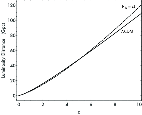
Figure 4: The luminosity distance as a function of redshift for $\Lambda$CDM (solid curve) and $R_{\rm h}=ct$ (dashed curve).

We ignore the Compton reflection of X-rays by the disk since the effect is minimal in the soft X-ray band (Magdziarz & Zdziarski 1995; Markoff, Melia & Sarcevic 1997; Trap et al. 2011). To keep the analysis as simple as possible, we also ignore absorption due to interactions with the surrounding gas and dust. Our flux calculations and subsequent estimates on the number of observable quasars should therefore be taken as upper limits. However, the results of Pezzulli et al. (2017) indicate that even if absorption is important, the overall effect out to $z\sim 10$ is not expected to be severe enough to impact our results.

4 Black-hole evolution and the resulting X-ray flux

We now combine the mass-growth model developed in §2 with the emission model from §3 in order to determine the observable flux of black holes evolving in $\Lambda$CDM and $R_{\rm h}=ct$. For illustrative purposes, we first apply our model to the sample of observed quasars highlighted in Nanni et al. (2017) with the best counting statistics in X-rays: J0100+2802, J1030+0524, J1120+0641, J1148+5251, and J1306+0356. The values of $z$, $M_{BH}$, and $\lambda_{\rm Edd}$ for these sources are reproduced in Table 1. The adopted mass for J1120+0641 is based on observations of the MgII line, while the mass and Eddington ratio for J1030+0524 and J1306+0356 were obtained by averaging the results presented in Table 4 of de Rosa et al. (2011), based on the use of their Equation 4. The radiative efficiency is assumed to be $\epsilon_{r}=0.1$ in all cases. We calculate the observed flux in the $0.5-2$ keV soft X-ray band as a function of redshift. The color coded results are shown in figure 5 for $\Lambda$CDM and figure 6 for $R_{\rm h}=ct$, with data points representing the $0.5-2$ keV fluxes derived by Nanni et al. (2017) based on Chandra observations.

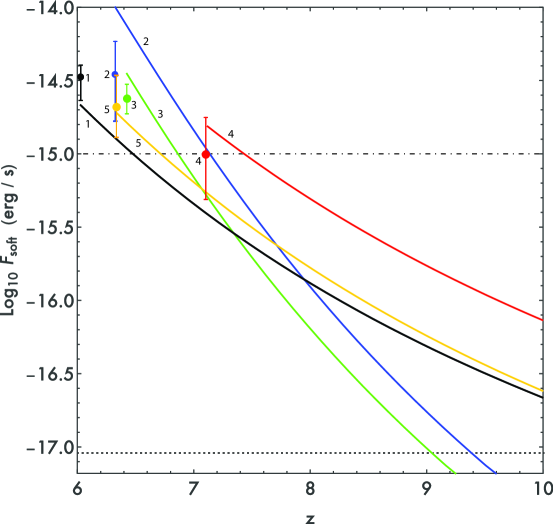
Figure 5: Soft X-ray band ($0.5-2$ keV) flux observed at Earth as a function of redshift in our $\Lambda$CDM evolutionary scenario, for 5 observed quasars highlighted in Nanni et al. (2017) with the best counting statistics in X-rays: J0100+2802 (blue,2), J1030+0524 (orange,5), J1120+0641 (red,4), J1148+5251 (green,3), and J1306+0356 (black,1). Data points represent the $0.5-2$ keV fluxes derived by Nanni et al. (2017) based on Chandra observations, together with their $1\sigma$ error bars. The dotted line represents the Chandra Deep Field South soft X-ray band flux limit of $9.1\times 10^{-18}$ erg/s, while the dot-dashed line represents the lowest observed soft X-ray flux in our sample of quasars taken from Nanni et al. (2017).

Table 1: X-ray Detected Quasars

Quasar	$z$	$M_{BH}$ ($M_{\odot}$)	$\lambda_{Edd}$	Reference
J1306+0356	6.0	$2.3\times 10^{9}$	0.45	De Rosa et al. (2011)
J0100+2802	6.3	$1.2\times 10^{10}$	1.06	Wu et al. (2015)
J1030+0524	6.3	$2.2\times 10^{9}$	0.5	De Rosa et al. (2011)
J1148+5251	6.4	$3.0\times 10^{9}$	1.0	Willott et al. (2003)
J1120+0641	7.1	$2.4\times 10^{9}$	0.5	De Rosa et al. (2014)

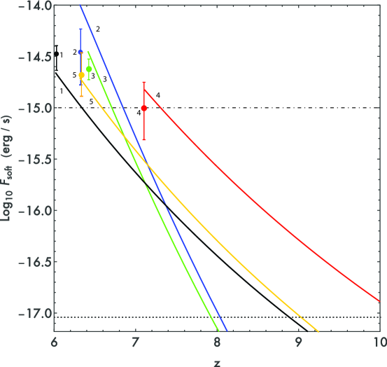
Figure 6: Soft X-ray band ($0.5-2$ keV) flux observed at Earth as a function of redshift in $R_{\rm h}=ct$, for 5 observed quasars highlighted in Nanni et al. (2017) with the best counting statistics in X-rays: J0100+2802 (blue,2), J1030+0524 (orange,5), J1120+0641 (red,4), J1148+5251 (green,3), and J1306+0356 (black,1). Data points represent the $0.5-2$ keV fluxes derived by Nanni et al. (2017) based on $Chandra$ observations, together with their $1\sigma$ error bars. The dotted line represents the Chandra Deep Field South soft X-ray band flux limit of $9.1\times 10^{-18}$ erg/s, while the dot-dashed line represents the lowest observed soft X-ray flux in our sample of quasars taken from Nanni et al. (2017).

Our results, which are in fairly good agreement with the observations, indicate that the difference in timelines between $\Lambda$CDM and $R_{\rm h}=ct$ has clear implications for the observability of quasars between redshifts $6-10$. In $\Lambda$CDM, assuming the quasars used in our analysis are representative of the broader population, a significant fraction of their counterparts would produce a soft X-ray flux above the lowest observed flux in our sample (dot-dashed line) between redshifts $z\approx 7-7.5$, and would produce a soft X-ray flux above the Chandra Deep Field South limit (dotted line) out to $z\sim 10$. The situation is considerably different in $R_{\rm h}=ct$, where relatively few quasars would be detected above our established sample threshold (dot-dashed line) out to a redshift of $z\approx 7.5$, and detection at the Chandra Deep Field South limit would be rare for $z\gtrsim 10$.

While figures 5 and 6 provide an important insight into how SMBHs evolve in both cosmologies, we wish to put our analysis on a firmer statistical footing. The recent (and ongoing) discovery, imaging and spectroscopic analysis of quasars at $z\approx 6$ now allows us to carry out a statistical analysis of their properties over a range of luminosities, and has lead to a determination of the quasar mass function at $z=6$. Specifically, the analysis of Willott et al. (2010), based on the absolute magnitude at 1450 $\AA$ for a sample of $z\approx 6$ quasars, yielded a Schechter mass function of the form

$$\Phi_{M}[M_{\rm bh};z=6]=\Phi_{0}\left({M_{\rm bh}\over M^{*}}\right)^{\alpha}e^{-M_{\rm bh}/M^{*}}\,,$$ (17)

with best fit parameters $\Phi_{0}=1.23\times 10^{-8}$ Mpc^-3 dex^-1, $M^{*}=2.24\times 10^{9}$ $M_{\odot}$, and $\alpha=-1.03$. This mass function normalized to yield the number of quasars $dN(M_{\rm bh},z)$ per mass dex between redshift $z$ and $z+dz$, evaluated at $z=6$, is shown in figure 7 for both cosmologies.

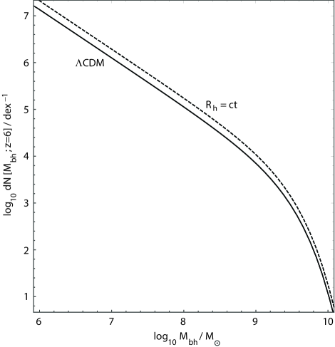
Figure 7: The mass function normalized to yield the number of quasars $dN(M_{\rm bh},z)$ per mass dex between redshift $z$ and $z+dz$, evaluated at $z=6$, for both cosmologies.

To keep our analysis as direct as possible, we use the fairly narrow distribution in $\lambda_{\rm Edd}$ values observed at $z\approx 6$ (see fig. 6 in Willott et al. 2010) as justification for setting $\lambda_{\rm Edd}=1$ for all quasars in the early Universe. In the absence of mergers, and with accretion occurring at the Eddington rate, all black holes evolve lock-step during the early Universe, and the mass function at any redshift can be easily obtained through the transformation

$$\Phi_{M}[M_{\rm bh};z]=\Phi_{M}[M_{\rm bh}e^{{(1-\epsilon_{r})\over\epsilon_{r}}{\lambda_{\rm Edd}\over t_{\rm Edd}}(t_{6}-t_{z})}\,;z=6]\,,$$ (18)

where $t_{z}$ is the age of the Universe at redshift $z$ (see Eqns.  2–4).

In order to assess the detectability of quasars at higher redshift for both cosmologies under consideration, we convert the luminosity function to a flux function at values of $z$ = 6, 7 and 8 for each model. The results are shown in figure 8, with the solid curves representing the $\Lambda$CDM case and the dashed curves representing the $R_{\rm h}=ct$ case. Note that the slight mismatch at $z$ = 6 results from the slight difference in luminosity distance between the two cases, which, as discussed above, was not corrected for. As can be clearly seen, a significantly smaller fraction of the quasars detected at $z=6$ can also be seen at higher redshifts for $R_{\rm h}=ct$ than for $\Lambda$CDM. This result stems almost entirely from the difference in mass growth between the two scenarios. For example, a time of 0.17 Gyr passes between $z=7$ and $z=6$ in $\Lambda$CDM, while the corresponding span of time is 0.26 Gyr in $R_{\rm h}=ct$. At $z=6$, a SMBH with mass $M_{\rm bh}=1.5\times 10^{6}\;M_{\odot}$ produces a soft X-ray flux at the Chandra limit. That result does not change much at $z=7$ for either Universe, since the luminosity distance changes by less than 25%. However, a SMBH evolving from $z=7$ to $z=6$ increases its mass by a factor of 30 in $\Lambda$CDM, and a factor of 180 in $R_{\rm h}=ct$. The corresponding shift in the mass function, as expressed by Equation (18), is therefore much greater in the $R_{\rm h}=ct$ universe.

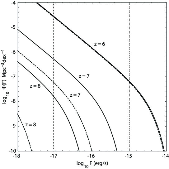
Figure 8: Flux distributions for $\Lambda$CDM (solid) and $R_{\rm h}=ct$ (dashed) at $z=6,7$ and 8. The dotted line represents the Chandra Deep Field South soft X-ray band flux limit of $9.1\times 10^{-18}$ erg/s, and the dot-dashed line represents the observed soft X-ray flux of the lowest mass SMBH in the sample used to generate figures 5 and 6, as calculated by our model.

To further illustrate this point, we next determine what fraction of quasars that produce a flux above the Chandra soft X-ray band limit at $z=6$ would still do so at higher redshifts. As noted above, a black hole at $z=6$ would need a mass of $M_{\rm bh}=1.5\times 10^{6}\;M_{\odot}$ to produce a flux equal to the Chandra Deep Field South soft X-ray band flux limit in our accretion model. Taking as our parent population all black holes at $z=6$ with mass greater than this limit, we then find the corresponding masses for which the population of black holes with a greater mass represent 80, 60, 40, 20, 10, 1 and 0.1%, respectively, of the parent population. For each of these demarking masses, we then calculate the flux evolution, as was done for figures 5 and 6, using the same parameters $\epsilon_{r}=0.1$ and $\lambda_{\rm Edd}=1$. The results are displayed in figure 9 for $\Lambda$CDM and figure 10 for $R_{\rm h}=ct$. In $\Lambda$CDM, 10% of our parent population would be observable (above the Chandra limit) beyond a redshift of $z\approx 6.55$, and only around 1% would be observable beyond redshift $z\gtrsim 7$. In contrast, for $R_{\rm h}=ct$, 10% of our parent population would be observable beyond a redshift of $z\approx 6.35$, and the most massive 1% would be observable beyond a redshift of $z\approx 6.7$. These results indicate that the next generation of observations, which should be able to provide a statistically significant number of $z\gtrsim 7$ detections, will be able to differentiate between $\Lambda$CDM and $R_{\rm h}=ct$. In both cases, only the most massive 0.1% of quasars produce a flux comparable to the minimum observed flux from our Nanni et al. (2017) sample used for Figures 5 and 6 (dot-dashed line) at a redshift of $z\sim 6$.

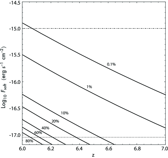
Figure 9: Chandra soft X-ray flux versus $z$ tracks in $\Lambda$CDM for quasars with black hole masses that demark 80, 60, 40, 20, 10, 1 and 0.1% of the parent population of all quasars with a mass greater than $1.5\times 10^{6}\;M_{\odot}$ at $z=6$, corresponding to the mass limit that produces a flux at that redshift equal to the Chandra Deep Field South soft X-ray band flux limit of $9.1\times 10^{-18}$ erg/s (indicated by the dotted line). The dot-dashed line represents the observed soft X-ray flux of the lowest mass SMBH in our sample used for figs. 5 and 6.

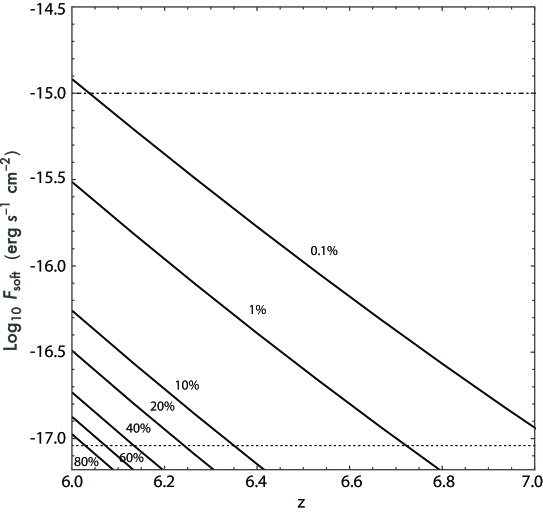
Figure 10: Chandra soft X-ray flux versus $z$ tracks in $R_{\rm h}=ct$ for quasars with black hole masses that demark 80, 60, 40, 20, 10, 1 and 0.1% of the parent population of all quasars with a mass greater than $1.5\times 10^{6}\;M_{\odot}$ at $z=6$, which corresponds to the mass limit that produces a flux at that redshift equal to the Chandra Deep Field South soft X-ray band flux limit of $9.1\times 10^{-18}$ erg/s (indicated by the dotted line). The dot-dashed line represents the observed soft X-ray flux of the lowest mass SMBH in our sample used for figures 5 and 6.

We conclude this analysis by estimating how many quasars should be detectable above a given flux threshold as a function of redshift by integrating the quasar mass function above that threshold out to $z=10$. This number is given by the integral expression

$$N(\geq F;z)\equiv\int_{z}^{10}\int_{\log_{10}[M_{t}(z^{\prime})]}^{\infty}\Phi(M_{\rm bh},z^{\prime})V_{z^{\prime}}\,d[\log_{10}(M_{\rm bh})]\,dz^{\prime}\,,$$ (19)

where $V_{z}=4\pi D_{c}^{2}\,dD_{c}/dz$ is the comoving differential volume and $M_{t}(z)$ represents the black hole mass at redshift $z$ required to produce a soft X-ray flux equal to $F$. Note that the comoving distance $D_{c}$ is smaller than the luminosity distance by a factor $(1+z)$. The results are presented in figure 11. As noted already, there is a significant difference in the expected number of detectable quasars predicted by the two cosmological models.

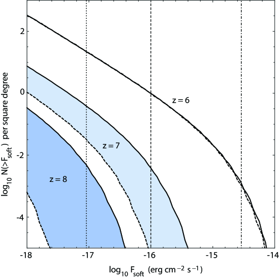
Figure 11: Number (density per square degree) of quasars that should be detectable above a given flux threshold $F_{\rm soft}$ as a function of that threshold for $z=6$, 7, and 8. At $z=6$, both $\Lambda$CDM and $R_{\rm h}=ct$ predict the same value because the curves are normalized to the observed luminosity function at that redshift. At larger redshifts, $\Lambda$CDM is indicated by the solid curve, while $R_{\rm h}=ct$ is shown with a dashed curve. The colored regions emphasize the differences between these two models at $z=7$ and 8. The dotted line represents the Chandra Deep Field South soft X-ray band flux limit of $9.1\times 10^{-18}$ erg/s, the dashed line represents the expected Athena flux limit, and the dot-dashed line represents the soft band (0.5 - 2 keV) point-source sensitivity for eROSITA at $\sim 140$ deg².

Based on the observed luminosity function at $z=6$, which is used to normalize the expected number of detectable quasars in both models, our analysis indicates that there is a steep drop off in the number of quasars that can be observed at $z\sim 7$ compared to $z\sim 6$ at flux limits greater than $\gtrsim 10^{-15}$ erg s^-1 cm^-2. As noted above, a SMBH evolving from $z=7$ to $z=6$ increases its mass by a factor of 30 in $\Lambda$CDM, and a factor of 180 in $R_{\rm h}=ct$. Similar to what was seen in Figure 8, the result is a more pronounced downward (leftward) shift (by about an order of magnitude) in the $R_{h}=ct$ curve than its $\Lambda$CDM counterpart at $z=7$ compared to their common $z=6$ curves. But the turnover in the mass distribution function acts to amplify the observational consequences between the two cosmologies. With a flux sensitivity $\gtrsim 3\times 10^{-15}$ erg s^-1 cm^-2 (represented by the dot-dashed vertical line in Figure 11), it seems very unlikely that eROSITA will be able to provide the observational evidence needed to discriminate between the two cosmological models under consideration. In contrast, the roughly three orders of magnitude difference in the number of $z\sim 7$ quasars that can be observed in $R_{\rm h}=ct$ versus $\Lambda$CDM for the ATHENA flux sensitivity (represented by the dashed vertical line in Figure 11) makes it quite likely that the observations made by that instrument will be able to discriminate between the two cosmologies in the next decade. Specifically, while we expect that ATHENA will detect very few, if any, quasars at $z\sim 7$ in $R_{h}=ct$, it should detect several hundred of them in $\Lambda$CDM—a rather compelling quantitative difference.

5 Conclusions

The detection of billion-solar-mass quasars at $z\gtrsim 6$ has created some tension with the Planck $\Lambda$CDM model, in the sense that conventional Eddington-limited accretion, as we understand it in the local Universe, could not have produced such large objects in the scant $400-500$ Myr afforded them by the timeline in this cosmology. Remedies to circumvent this problem have included models to create $\sim 10^{5}\;M_{\odot}$ seeds or to permit transient super-Eddington accretion, requiring a very low duty-cycle. Both of these solutions are anomalous because no evidence for either of them has ever been seen. In fact, the quasar luminosity function towards $z\sim 6$ suggests that the inferred accretion rate saturates at close to the Eddington value, with a spread no greater than about 0.3 dex. The data seem to be telling us that these supermassive black holes probably grew to their observed size near $z=6$ by accreting more or less steadily at roughly the Eddington value.

In previous work, we demonstrated that an alternative, perhaps more elegant, solution to this problem may simply be to replace the timeline in $\Lambda$CDM with that in the $R_{\rm h}=ct$ universe. By now, these two models have been compared with each other and tested against the observations using over 20 different kinds of data. The $R_{\rm h}=ct$ model has not only passed all of these tests, but has actually been shown to account for the data analyzed thus far better than the standard model. There is therefore ample motivation to advance the study of SMBH evolution in this cosmology beyond mere demographics.

This has been the goal of this paper—to examine the progenitor statistics in both models, based on the observed luminosity function at $z\sim 6$. We have sought to keep the analysis as simple and straightforward as possible, avoiding unnecessarily complicated SED contributions. For this purpose, the $0.5-2.0$ keV flux, thought to be produced in the corona overlying the accretion disk, appears to be an ideal spectral component. The model for producing this emissivity is simple, and probably reliable over a large range in black-hole mass. In addition, one can easily compensate for a transition in the accretion rate, from low to large values.

With this basic accretion model, we have demonstrated that—for the two cosmologies examined here—the difference in the expected number of detections with the upcoming ATHENA mission is very large. According to figure 11, and based on the observed luminosity function at $z\sim 6$, the ATHENA mission is expected to detect approximately $3.9\times 10^{-6}$ quasars per square degree at $z\sim 7$ in $R_{\rm h}=ct$, i.e., approximately $0.16$ over the whole sky. By comparison, this number is $\sim 3.9\times 10^{-3}$ quasars per square degree at $z\sim 7$ in $\Lambda$CDM, or roughly $160$ over the whole sky.

The caveat, of course, is that we have ignored the impact of mergers throughout this analysis. Superficially, one could reasonably expect that the merger rate should be about the same in both cosmologies. Nonetheless, the numbers shown in figure 11 should be viewed as upper limits. One also needs to take into account the fact that an observed detection rate lower than that predicted by $\Lambda$CDM may be partially due to SMBH growth via these mergers, rather than it being a strong indication that the timeline in $R_{\rm h}=ct$ is preferred by the data. On the flip side, mergers cannot lead to a detection rate much higher than that shown in figure 11, depending on how reliable our streamlined accretion model happens to be. Thus, if the number of high-$z$ quasars detected with future surveys is closer to that predicted by $\Lambda$CDM (i.e., the solid curves in this figure), this would argue strongly against $R_{\rm h}=ct$, particularly at $z\sim 8$, where the difference is expected to be even more pronounced.

References

- (1) Abramowicz M. A., Czerny B., Lasota J. P., Szuszkiewicz E., 1988, ApJ, 332, 646
- (2) Ade, P.A.R. et al., 2016, A&A, 594, id A13
- (3) Brightman, M., et al., 2013, MNRAS, 433, 2485
- (4) Chan, C.-K., Liu, S., Fryer, C. L., Psaltis, D., Özel, F., Rockefeller, G. & Melia, F. 2009, ApJ, 701, 521
- (5) de Rosa, G., et al. 2011, ApJ, 739, 56
- (6) de Rosa, G., et al. 2014, ApJ, 790, 145
- (7) Fiore, F., et al., 2009, ApJ, 693, 447
- (8) Georgakakis, A., et al., 2015, MNRAS, 453, 1946
- (9) Liu, S. & Melia, F., 2001, ApJL, 561, L77
- (10) Lusso, E., Risaliti, G., 2016, ApJ, 819, 154
- (11) Madau, P., Haardt, F., Dotti, M., 2014, ApJ, 784, L38
- (12) Magdziarz, P., Zdziarski, A. A., 1995, MNRAS, 273, 837
- (13) Markoff, S., Melia, F. & Sarceivc, I., 1997, ApJL, 489, L47
- (14) Melia, F., 2013, ApJ, 764, 72
- (15) Melia, F., 2014, A&A, 561, A80
- (16) Melia, F., 2017, MNRAS, 464, 1966
- (17) Melia, F. & Fatuzzo, M., 2016, MNRAS, 456, 3422
- (18) Melia, F. and Maier, R. S., 2013, MNRAS, 432, 2669
- (19) Melia, F. and McClintock, T. M., 2015, Proc. R. Soc. A, 471, 20150449
- (20) Melia, F., Wei, J.-J., Wu, X.-F., 2015, AJ, 149, 2
- (21) Mortlock, D. J. et al., 2011, Nature, 474, 616
- (22) Nanni, R., Vignali, C, Gilli, R., Moretti, A. and Brandt, W. N., 2017, arXiv: 1704.08693
- (23) Pezzulli, E., Valiente, R., Orofino, M., Schneider, R., Sbarrato, T., 2017, MNRAS, 466, 2131
- (24) Ruffert, M. & Melia, F., 1994, A&A, 288L, L29
- (25) Shakura N. I., Sunyaev R. A., 1973, A&A, 24, 337
- (26) Trap, G., Goldwurm, A., Dodds-Eden, K., Weiss, A., Terrier, R., Ponti, G., Gillessen, S., Genzel, R., Ferrando, P., Bélanger, G. et al. 2011, A&A, 528, id.A140
- (27) Treister, E., Schawinski, K., Volonteri, M., Natarajan, P., 2013, ApJ, 778, 130
- (28) Volonteri, M. and Rees, M. J., 2005, ApJ, 633, 624
- (29) Volonteri, M., Silk, J. and Dubus, G., 2015, ApJ, 804, 148
- (30) Wei, J.-J., Wu, X.-F. and Md Melia, F., 2014b, ApJ, 788, 190
- (31) Wei, J.-J., Wu, X.-F., Melia, F. and Maier, R. S., 2015a, AJ, 149, 102
- (32) Wei, J.-J., Wu, X.-Felia, F., 2013, ApJ, 772, 43
- (33) Wei, J.-J., Wu, X.-F., Melia, F., Wei, D.-M. and Feng, L.-L., 2014a, MNRAS, 439, 3329
- (34) Wei, J.-J., Wu, X.-F. an. and Melia, F., 2015b, MNRAS, 447, 479
- (35) Weigel, A. K., Schawinski, K., Treister, E., Urry, C. M. and Koss, M. and Trakhtenbrot, B., 2015, MNRAS, 448, 3167
- (36) Willott, C. J., McLure, R. J. and Jarvis, M.J., 2003, ApJ Letters, 587, L15
- (37) Willott, C. J. et al., 2010, AJ, 140, 546
- (38) Wu, X.-B., et al. 2015, Nature, 518, Issue 7540, 512
- (39) Yoo, J. and Miralda-Escudé J., 2004, ApJ, 614, L25