On multilevel Picard numerical approximations
for high-dimensional nonlinear parabolic partial
differential equations and high-dimensional nonlinear
backward stochastic differential equations

Abstract

Parabolic partial differential equations (PDEs) and backward stochastic differential equations (BSDEs) are key ingredients in a number of models in physics and financial engineering. In particular, parabolic PDEs and BSDEs are fundamental tools in the state-of-the-art pricing and hedging of financial derivatives. The PDEs and BSDEs appearing in such applications are often high-dimensional and nonlinear. Since explicit solutions of such PDEs and BSDEs are typically not available, it is a very active topic of research to solve such PDEs and BSDEs approximately. In the recent article [E, W., Hutzenthaler, M., Jentzen, A., & Kruse, T. Linear scaling algorithms for solving high-dimensional nonlinear parabolic differential equations. arXiv:1607.03295 (2017)] we proposed a family of approximation methods based on Picard approximations and multilevel Monte Carlo methods and showed under suitable regularity assumptions on the exact solution for semilinear heat equations that the computational complexity is bounded by $O(d\,{\varepsilon}^{-(4+\delta)})$ for any $\delta\in(0,\infty)$, where $d$ is the dimensionality of the problem and ${\varepsilon}\in(0,\infty)$ is the prescribed accuracy. In this paper, we test the applicability of this algorithm on a variety of $100$-dimensional nonlinear PDEs that arise in physics and finance by means of numerical simulations presenting approximation accuracy against runtime. The simulation results for these 100-dimensional example PDEs are very satisfactory in terms of accuracy and speed. In addition, we also provide a review of other approximation methods for nonlinear PDEs and BSDEs from the literature.

1 Introduction and main results

Parabolic partial differential equations (PDEs) and backward stochastic differential equations (BSDEs) have a wide range of applications. To give specific examples we focus now on a number of applications in finance. There are several fundamental assumptions incorporated in the Black-Scholes model that are not met in the real-life trading of financial derivatives. A number of derivative pricing models have been developed in about the last four decades to relax these assumptions; see, e.g., [9, 29, 8, 62, 42, 59, 18] for models taking into account the fact that the “risk-free” bank account has higher interest rates for borrowing than for lending, particularly, due to the default risk of the trader, see, e.g., [53, 18] for models incorporating the default risk of the issuer of the financial derivative, see, e.g., [82, 6, 5] for models for the pricing of financial derivatives on underlyings which are not tradeable such as financial derivatives on the temperature or mortality-dependent financial derivatives, see, e.g., [1] for models incorporating that the hedging strategy influences the price processes through demand and supply (so-called large investor effects), see, e.g., [33, 61, 48] for models taking the transaction costs in the hedging portfolio into account, and see, e.g., [2, 48] for models incorporating uncertainties in the model parameters for the underlying. In each of the above references the value function $u$, describing the price of the financial derivative, solves a nonlinear parabolic PDE. Moreover, the PDEs for the value functions emerging from the above models are often high-dimensional as the financial derivative depends in several cases on a whole basket of underlyings and as a portfolio containing several financial derivatives must often be treated as a whole in the case where the above nonlinear effects are taken into account (cf., e.g., [18, 33, 8]). These high-dimensional nonlinear PDEs can typically not be solved explicitly and, in particular, there is a strong demand from the financial engineering industry to approximately compute the solutions of such high-dimensional nonlinear parabolic PDEs.

The numerical analysis literature contains a number of deterministic approximation methods for nonlinear parabolic PDEs such as finite element methods, finite difference methods, spectral Galerkin approximation methods, or sparse grid methods (cf., e.g., [80, Chapter 14], [79, Section 3], [78], and [73]). Some of these methods achieve high convergence rates with respect to the computational effort and, in particular, provide efficient approximations in low or moderate dimensions. However, these approximation methods can not be used in high dimensions as the computational effort grows exponentially in the dimension $d\in{\mathbbm{N}}=\{1,2,\dots\}$ of the considered nonlinear parabolic PDE and then the method fails to terminate within years even for low accuracies.

In the case of linear parabolic PDEs the Feynman-Kac formula establishes an explicit representation of the solution of the PDE as the expectation of the solution of an appropriate stochastic differential equation (SDE). (Multilevel) Monte Carlo methods together with suitable discretizations of the SDE (see, e.g., [68, 58, 57, 56]) then result in a numerical approximation method with a computational effort that grows at most polynomially in the dimension $d\in{\mathbbm{N}}$ of the PDE and that grows up to an arbitrarily small order quadratically in the reciprocal of the approximation precision (cf., e.g., [46, 39, 49, 50]). These multilevel Monte Carlo approximations are, however, limited to linear PDEs as the classical Feynman-Kac formula provides only in the case of a linear PDE an explicit representation of the solution of the PDE. For lower error bounds in the literature on random and deterministic numerical approximation methods for high-dimensional linear PDEs the reader is, e.g., referred to Heinrich [51, Theorem 1].

In the seminal papers [71, 72, 70], Pardoux & Peng developed the theory of nonlinear backward stochastic differential equations and, in particular, established a considerably generalized nonlinear Feynman-Kac formula to obtain an explicit representation of the solution of a nonlinear parabolic PDE by means of the solution of an appropriate BSDE; see also Cheridito et al. [17] for second-order BSDEs. Discretizations of BSDEs, however, require suitable discretizations of nested conditional expectations (see, e.g., [10, 83, 32, 47, 17]). Discretization methods for these nested conditional expectations proposed in the literature include the ’straight forward’ Monte Carlo method, the quantization tree method (see [4]), the regression method based on Malliavin calculus or based on kernel estimation (see [10]), the projection on function spaces method (see [42]), the cubature on Wiener space method (see [22]), and the Wiener chaos decomposition method (see [12]). None of these discretization methods has the property that the computational effort of the method grows at most polynomially both in the dimension and in the reciprocal of the prescribed accuracy (see Subsections 4.1–4.6 below for a detailed discussion). We note that solving high-dimensional semilinear parabolic PDEs at single space-time points and solving high-dimensional nonlinear BSDEs at single time points is essentially equivalent due to the generalized nonlinear Feynman-Kac formula established by Pardoux & Peng. In recent years the concept of fractional smoothness in the sense of function spaces has been used for studying variational properties of BSDEs. This concept of fractional smoothness quantifies the propagation of singularities in time and shows that certain non-uniform time grids are more suitable in the presence of singularities; see, e.g., Geiss & Geiss [36], Gobet & Makhlouf [43] or Geiss, Geiss, & Gobet [35] for details. Also these temporal discretization methods require suitable discretizations of nested conditional expectations resulting in the same problems as in the case of uniform time grids.

Another probabilistic representation for solutions of some nonlinear parabolic PDEs with polynomial nonlinearities has been established in Skorohod [77] by means of branching diffusion processes. Recently, this classical representation has been extended under suitable assumptions in Henry-Labordère [53] to more general analytic nonlinearities and in Henry-Labordère et al. [54] to polynomial nonlinearities in the pair $(u(t,x),(\nabla_{x}u)(t,x))\in{\mathbbm{R}}^{1+d}$, $(t,x)\in[0,T]\times{\mathbbm{R}}^{d}$, where $u$ is the solution of the PDE, $d\in{\mathbbm{N}}$ is the dimension, and $T\in(0,\infty)$ is the time horizon. This probabilistic representation has been successfully used in Henry-Labordère [53] (see also Henry-Labordère, Tan, & Touzi [55]) and in Henry-Labordère et al. [54] to obtain a Monte Carlo approximation method for semilinear parabolic PDEs with a computational complexity which is bounded by $O(d\,{\varepsilon}^{-2})$ where $d$ is the dimensionality of the problem and ${\varepsilon}\in(0,\infty)$ is the prescribed accuracy. The major drawback of the branching diffusion method is its insufficient applicability, namely it requires the terminal/initial condition of the parabolic PDE to be quite small (see Subsection 4.7 below for a detailed discussion).

In the recent article [28] we proposed a family of approximation methods which we denote as multilevel Picard approximations (see (8) for its definition and Section 2 for its derivation). Corollary 3.18 in [28] shows under suitable regularity assumptions (including smoothness and Lipschitz continuity) on the exact solution that the computational complexity of this algorithm is bounded by $O(d\,{\varepsilon}^{-(4+\delta)})$ for any $\delta\in(0,\infty)$, where $d$ is the dimensionality of the problem and ${\varepsilon}\in(0,\infty)$ is the prescribed accuracy. In this paper we complement the theoretical complexity analysis of [28] with a simulation study. Our simulations in Section 3 indicate that the computational complexity grows at most linearly in the dimension and quartically in the reciprocal of the prescribed accuracy also for several $100$-dimensional nonlinear PDEs from physics and finance with non-smooth and/or non-Lipschitz nonlinearities and terminal condition functions. The simulation results for these $100$-dimensional example PDEs are very satisfactory in terms of accuracy and speed.

1.1 Notation

Throughout this article we frequently use the following notation. We denote by $\langle\cdot,\cdot\rangle\colon\left(\cup_{n\in{\mathbbm{N}}}({\mathbbm{R}}^{n}\times{\mathbbm{R}}^{n})\right)\to[0,\infty)$ the function that satisfies for all $n\in{\mathbbm{N}}$, $v=(v_{1},\dots,v_{n})$, $w=(w_{1},\dots,w_{n})\in{\mathbbm{R}}^{n}$ that $\langle v,w\rangle=\sum_{i=1}^{n}v_{i}w_{i}$. For every topological space $(E,\mathcal{E})$ we denote by $\mathcal{B}(E)$ the Borel-sigma-algebra on $(E,\mathcal{E})$. For all measurable spaces $(A,\mathcal{A})$ and $(B,\mathcal{B})$ we denote by $\mathcal{M}(\mathcal{A},\mathcal{B})$ the set of $\mathcal{A}$/$\mathcal{B}$-measurable functions from $A$ to $B$. For every probability space $(\Omega,\mathcal{A},{\mathbb{P}})$ we denote by $\left\|\cdot\right\|_{L^{2}({\mathbb{P}};{\mathbbm{R}})}\colon\mathcal{M}(\mathcal{A},\mathcal{B}({\mathbbm{R}}))\to[0,\infty]$ the function that satisfies for all $X\in\mathcal{M}(\mathcal{A},\mathcal{B}({\mathbbm{R}}))$ that $\|X\|_{L^{2}({\mathbb{P}};{\mathbbm{R}})}=\sqrt{{\mathbb{E}}\!\left[|X|^{2}\right]}$. For all metric spaces $(E,d_{E})$ and $(F,d_{F})$ we denote by ${\operatorname{Lip}}(E,F)$ the set of all globally Lipschitz continuous functions from $E$ to $F$. For every $d\in{\mathbbm{N}}$ we denote by $\operatorname{I}_{{\mathbbm{R}}^{d\times d}}$ the identity matrix in ${\mathbbm{R}}^{d\times d}$ and we denote by ${\mathbbm{R}}^{d\times d}_{\operatorname{Inv}}$ the set of invertible matrices in ${\mathbbm{R}}^{d\times d}$. For every $d\in{\mathbbm{N}}$ and every $A\in{\mathbbm{R}}^{d\times d}$ we denote by $A^{*}\in{\mathbbm{R}}^{d\times d}$ the transpose of $A$. For every $d\in{\mathbbm{N}}$ and every $x=(x_{1},\ldots,x_{d})\in{\mathbbm{R}}^{d}$ we denote by $\operatorname{diag}(x)\in{\mathbbm{R}}^{d\times d}$ the diagonal matrix with diagonal entries $x_{1},\ldots,x_{d}$. For every $T\in(0,\infty)$ we denote by $\mathcal{Q}_{T}$ the set given by $\mathcal{Q}_{T}=\{w\colon[0,T]\to{\mathbbm{R}}\colon w^{-1}({\mathbbm{R}}\backslash\{0\})\text{ is a finite set}\}$. We denote by $\lfloor\cdot\rfloor\colon{\mathbbm{R}}\to{\mathbbm{Z}}$ and $[\cdot]^{+}\colon{\mathbbm{R}}\to[0,\infty)$ the functions that satisfy for all $x\in{\mathbbm{R}}$ that $\lfloor x\rfloor=\max({\mathbbm{Z}}\cap(-\infty,x])$ and $[x]^{+}=\max\{x,0\}$.

2 Multilevel Picard approximations for high-dimensional semilinear PDEs

In Subsection 2.3 below we define multilevel Picard approximations (see (8) below) in the case of semilinear PDEs (cf. (5) in Subsection 2.2 below). These approximations have been introduced in [28]. In Subsection 2.1 we explain the abstract idea behind multilevel Picard approximations. In Subsection 2.2 we derive a fixed-point equation for semilinear PDEs which is based on the Feynman-Kac and Bismut-Elworthy-Li formulas.

2.1 Abstract picture for multilevel Picard approximations

Roughly speaking, a key idea in our approach to solve high-dimensional nonlinear PDEs/BSDEs is to formulate the solution of the considered PDE/BSDE as the solution of a suitable fixed-point equation and then to approximate the fixed-point by suitable multilevel Picard approximations (see (4) below). We now first outline this idea in an abstract form (see (2)–(4) below) and, thereafter, we demonstrate (see Subsections 2.2–2.3) how this general idea is applied to high-dimensional semilinear PDEs and high-dimensional BSDEs.

Let $(\mathcal{V},\left\|\cdot\right\|_{\mathcal{V}})$ be an ${\mathbbm{R}}$-Banach space and let ${\bf\Phi}\colon\mathcal{V}\to\mathcal{V}$ be a contraction on $(\mathcal{V},\left\|\cdot\right\|_{\mathcal{V}})$. The Banach fixed-point theorem then ensures that there exists a unique fixed-point of ${\bf\Phi}$, that is, the Banach fixed-point theorem establishes the existence of a unique element ${\bf u}_{\infty}\in\mathcal{V}$ with the property that

$${\bf u}_{\infty}={\bf\Phi}({\bf u}_{\infty}).$$ (1)

We think of $\mathcal{V}$ as a suitable space of functions, we think of (1) as a suitable reformulation of the considered deterministic PDE, and we think of ${\bf u}_{\infty}\in\mathcal{V}$ as the pair consisting of the solution of the considered PDE and of its spatial derivative. Next let $({\bf u}_{k})_{k\in{\mathbbm{N}}_{0}}\subseteq\mathcal{V}$ be a sequence of fixed-point iterations associated to (1), i.e., let $({\bf u}_{k})_{k\in{\mathbbm{N}}_{0}}\subseteq\mathcal{V}$ satisfy for all $k\in{\mathbbm{N}}$ that ${\bf u}_{k}={\bf\Phi}({\bf u}_{k-1})$. In examples we choose $({\bf u}_{k})_{k\in{\mathbbm{N}}_{0}}\subseteq\mathcal{V}$ such that ${\bf u}_{0}$ is known explicitly or easily computable. The Banach fixed-point theorem also ensures that $\lim_{k\to\infty}{\bf u}_{k}={\bf u}_{\infty}$ and that this convergence happens exponentially fast. To introduce our multilevel Picard approximations, we need suitable computable approximations of the typically nonlinear function ${\bf\Phi}\colon\mathcal{V}\to\mathcal{V}$, that is, we consider a family $\Psi^{k,n}_{l,\rho}\colon\mathcal{V}\to\mathcal{V}$, $l,k\in{\mathbbm{N}}$, $n\in\{0,1\}$, $\rho\in(0,\infty)$, of functions on $\mathcal{V}$ and we think of $\Psi^{k,n}_{l,\rho}$ for $l,k\in{\mathbbm{N}}$, $n\in\{0,1\}$, $\rho\in(0,\infty)$ as appropriate computable approximations of ${\bf\Phi}$ in the sense that $\Psi^{k,0}_{l,\rho}$ and $\Psi^{k,1}_{l,\rho}$ get closer to ${\bf\Phi}$ in a suitable sense as $l\in{\mathbbm{N}}$ (and $k\in{\mathbbm{N}}$ and $\rho\in(0,\infty)$ respectively) gets larger. This, the fact that $\lim_{k\to\infty}{\bf u}_{k}={\bf u}_{\infty}$, and the fact that for all $k\in{\mathbbm{N}}$ it holds that ${\bf u}_{k}={\bf\Phi}({\bf u}_{k-1})$ then ensure for all sufficiently large $k\in{\mathbbm{N}}$ that

$$\begin{split}{\bf u}_{\infty}\approx{\bf u}_{k}={\bf u}_{1}+\sum_{l=1}^{k-1}\left[{\bf u}_{l+1}-{\bf u}_{l}\right]&={\bf\Phi}({\bf u}_{0})+\sum_{l=1}^{k-1}\Big{[}{\bf\Phi}({\bf u}_{l})-{\bf\Phi}({\bf u}_{l-1})\Big{]}\\ &\approx\Psi_{k,\rho}^{k,0}({\bf u}_{0})+\sum_{l=1}^{k-1}\Big{[}\Psi^{k,0}_{k-l,\rho}({\bf u}_{l})-\Psi^{k,1}_{k-l,\rho}({\bf u}_{l-1})\Big{]}.\end{split}$$ (2)

The first $\approx$ in (2) exploits the fact that $\lim_{k\to\infty}{\bf u}_{k}={\bf u}_{\infty}$ and the second $\approx$ in (2) uses our approximation assumption on $\Psi^{k,n}_{l,\rho}$, $l,k\in{\mathbbm{N}}$, $n\in\{0,1\}$, $\rho\in(0,\infty)$. Display (2) suggests to introduce suitable numerical approximations of ${\bf u}_{k}$, $k\in{\mathbbm{N}}$, and ${\bf u}_{\infty}$, respectively. More formally, let $\psi_{k,\rho}\colon\mathcal{V}^{k}\to\mathcal{V}$, $k\in{\mathbbm{N}}$, $\rho\in(0,\infty)$, be the functions which satisfy for all $k\in{\mathbbm{N}}$, $\rho\in(0,\infty)$, $v_{0},v_{1},\dots,v_{k-1}\in\mathcal{V}$ that

$$\psi_{k,\rho}(v_{0},v_{1},\dots,v_{k-1})=\sum_{l=0}^{k-1}\Big{[}\Psi_{k-l,\rho}^{k,0}\big{(}v_{l}\big{)}-\mathbbm{1}_{{\mathbbm{N}}}(l)\,\Psi_{k-l,\rho}^{k,1}\big{(}v_{[l-1]^{+}}\big{)}\Big{]}$$ (3)

and let ${\bf U}_{k,\rho}\in\mathcal{V}$, $k\in{\mathbbm{N}}_{0}$, $\rho\in(0,\infty)$, satisfy for all $k\in{\mathbbm{N}}$, $\rho\in(0,\infty)$ that ${\bf U}_{0,\rho}={\bf u}_{0}$ and

$${\bf U}_{k,\rho}=\psi_{k,\rho}\big{(}{\bf U}_{0,\rho},{\bf U}_{1,\rho},\dots,{\bf U}_{k-1,\rho}\big{)}=\sum_{l=0}^{k-1}\Big{[}\Psi^{k,0}_{k-l,\rho}\big{(}{\bf U}_{l,\rho}\big{)}-\mathbbm{1}_{{\mathbbm{N}}}(l)\,\Psi_{k-l,\rho}^{k,1}\big{(}{\bf U}_{[l-1]^{+},\rho}\big{)}\Big{]}.$$ (4)

We would like to point out that the approximations in (4) are full history recursive in the sense that for every $k\in{\mathbbm{N}}$ and every $\rho\in(0,\infty)$ the “full history” ${\bf U}_{0,\rho}$, ${\bf U}_{1,\rho}$, $\dots$, ${\bf U}_{k-1,\rho}$ needs to be computed recursively in order to compute ${\bf U}_{k,\rho}$. Moreover, we note that the approximations in (4) exploit multilevel/multigrid ideas (cf., e.g., [49, 52, 50, 39]). Typically multilevel ideas appear where the different levels correspond to approximations with different time or space step sizes while here different levels correspond to different stages of the fixed-point iteration. This, in turn, results in numerical approximations which require the full history of the approximations. A key feature of the approximations in (4) is that – depending on the choice of the space $(\mathcal{V},\left\|\cdot\right\|_{\mathcal{V}})$, the function ${\bf\Phi}$, and the functions $(\Psi^{k,n}_{l,\rho})_{l,k\in{\mathbbm{N}},n\in\{0,1\},\rho\in(0,\infty)}$ – the approximations (4) often preserve the frequently exceedingly high convergence speed of the $({\bf u}_{k})_{k\in{\mathbbm{N}}}$ to ${\bf u}_{\infty}$ while keeping the computational cost moderate compared to the desired approximation precision.

2.2 A fixed-point equation for semilinear PDEs

To get a better understanding of the approximation scheme introduced in Subsection 2.3, we present in this subsection a rough derivation of a fixed-point equation on which the scheme (8) is based on. For this fixed-point equation we impose for simplicity of presentation appropriate additional hypotheses that are not needed for the definition of the scheme (8) (cf. (5)–(7) in this subsection with Subsection 2.3).

Let $T\in(0,\infty)$, $d\in{\mathbbm{N}}$, let $g\colon{\mathbbm{R}}^{d}\to{\mathbbm{R}}$, $f\colon[0,T]\times{\mathbbm{R}}^{d}\times{\mathbbm{R}}\times{\mathbbm{R}}^{d}\to{\mathbbm{R}}$, $u\colon[0,T]\times{\mathbbm{R}}^{d}\to{\mathbbm{R}}$, $\eta\colon{\mathbbm{R}}^{d}\to{\mathbbm{R}}^{d}$, $\mu\colon[0,T]\times{\mathbbm{R}}^{d}\to{\mathbbm{R}}^{d}$, and $\sigma=(\sigma_{1},\ldots,\sigma_{d})\colon[0,T]\times{\mathbbm{R}}^{d}\to{\mathbbm{R}}^{d\times d}_{\operatorname{Inv}}$ be sufficiently regular functions, assume for all $t\in[0,T)$, $x\in{\mathbbm{R}}^{d}$ that $u(T,x)=g(x)$ and

$$(\tfrac{\partial}{\partial t}u)(t,x)+f\big{(}t,x,u(t,\eta(x)),[\sigma(t,\eta(x))]^{*}(\nabla_{x}u)(t,\eta(x))\big{)}+\langle\mu(t,x),(\nabla_{x}u)(t,x)\rangle\\ +\tfrac{1}{2}\operatorname{Trace}\!\big{(}\sigma(t,x)[\sigma(t,x)]^{*}(\operatorname{Hess}_{x}u)(t,x)\big{)}=0,$$ (5)

let $(\Omega,\mathcal{F},{\mathbb{P}},(\mathbb{F}_{t})_{t\in[0,T]})$ be a stochastic basis (cf., e.g., [74, Appendix E]), let $W=$ $(W^{1},\dots,$ $W^{d})\colon[0,T]\times\Omega\to{\mathbbm{R}}^{d}$ be a standard $(\mathbb{F}_{t})_{t\in[0,T]}$-Brownian motion, and for every $s\in[0,T]$, $x\in{\mathbbm{R}}^{d}$ let $X^{s,x}\colon[s,T]\times\Omega\to{\mathbbm{R}}^{d}$ and $D^{s,x}\colon[s,T]\times\Omega\to{\mathbbm{R}}^{d\times d}$ be $(\mathbb{F}_{t})_{t\in[s,T]}$-adapted stochastic processes with continuous sample paths which satisfy that for all $t\in[s,T]$ it holds ${\mathbb{P}}$-a.s. that

$$\begin{split}X^{s,x}_{t}&=x+\int_{s}^{t}\mu(r,X^{s,x}_{r})\,dr+\sum_{j=1}^{d}\int_{s}^{t}\sigma_{j}(r,X^{s,x}_{r})\,dW^{j}_{r},\\ D^{s,x}_{t}&=\operatorname{I}_{{\mathbbm{R}}^{d\times d}}+\int_{s}^{t}(\tfrac{\partial}{\partial x}\mu)(r,X^{s,x}_{r})\,D^{s,x}_{r}\,dr+\sum_{j=1}^{d}\int_{s}^{t}(\tfrac{\partial}{\partial x}\sigma_{j})(r,X^{s,x}_{r})\,D^{s,x}_{r}\,dW^{j}_{r}.\end{split}$$ (6)

For every $s\in[0,T]$ the processes $D^{s,x}$, $x\in{\mathbbm{R}}^{d}$, are in a suitable sense the derivative processes of $X^{s,x}$, $x\in{\mathbbm{R}}^{d}$ with respect to $x\in{\mathbbm{R}}^{d}$. The function $\eta$ in (5) allows to include a possible space shift in the PDE. Typically we are interested in the case where $\eta$ is the identity, that is, for all $x\in{\mathbbm{R}}^{d}$ it holds that $\eta(x)=x$. Our approximation scheme in (8) below is based on a suitable fixed-point formulation of the solution of the PDE (5). To obtain such a fixed-point formulation, we apply the Feynman-Kac formula and the Bismut-Elworthy-Li formula (see, e.g., Elworthy & Li [30, Theorem 2.1] or Da Prato & Zabczyk [25, Theorem 2.1]). More precisely, let ${\bf u}^{\infty}\in{\operatorname{Lip}}([0,T]\times{\mathbbm{R}}^{d},{\mathbbm{R}}^{1+d})$ satisfy for all $(t,x)\in[0,T)\times{\mathbbm{R}}^{d}$ that ${\bf u}^{\infty}(t,x)=\big{(}u(t,x),[\sigma(t,x)]^{*}(\nabla_{x}u)(t,x)\big{)}$ and let $\Phi\colon{\operatorname{Lip}}([0,T]\times{\mathbbm{R}}^{d},{\mathbbm{R}}^{1+d})\to{\operatorname{Lip}}([0,T]\times{\mathbbm{R}}^{d},{\mathbbm{R}}^{1+d})$ satisfy for all ${\bf v}\in{\operatorname{Lip}}([0,T]\times{\mathbbm{R}}^{d},{\mathbbm{R}}^{1+d})$, $(s,x)\in[0,T)\times{\mathbbm{R}}^{d}$ that

$$\begin{split}\big{(}\Phi({\bf v})\big{)}(s,x)&=\textstyle{\mathbb{E}}\!\left[\left(g(X^{s,x}_{T})-g(x)\right)\left(1,\tfrac{[\sigma(s,x)]^{*}}{T-s}\smallint\nolimits_{s}^{T}\big{[}\sigma(r,X_{r}^{s,x})^{-1}D_{r}^{s,x}\big{]}^{*}dW_{r}\right)\right]+\left(g(x),0\right)\\ &\quad\textstyle+\int_{s}^{T}{\mathbb{E}}\!\left[f\Big{(}t,X_{t}^{s,x},{\bf v}\big{(}t,\eta(X_{t}^{s,x})\big{)}\Big{)}\,\big{(}1,\tfrac{[\sigma(s,x)]^{*}}{t-s}\smallint\nolimits_{s}^{t}\big{[}\sigma(r,X_{r}^{s,x})^{-1}D_{r}^{s,x}\big{]}^{*}\,dW_{r}\big{)}\right]dt\end{split}$$ (7)

Combining (7) with the Feynman-Kac formula and the Bismut-Elworthy-Li formula ensures that ${\bf u}^{\infty}=\Phi({\bf u}^{\infty})$. Note that we have incorporated a zero expectation term in (7). The purpose of this term is to slightly reduce the variance when approximating the right-hand side of (7) by Monte Carlo approximations. Now we approximate the non-discrete quantities in (7) (expectation and time integral) by discrete quantities (Monte Carlo averages and quadrature formulas) with different degrees of discretization on different levels (cf. the remarks in Subsection 2.4 below). This yields a family of approximations of $\Phi$. With these approximations of $\Phi$ we finally define multilevel Picard approximations of ${\bf u}^{\infty}$ through (4) which results in the approximations (8).

2.3 The approximation scheme

In this subsection we introduce multilevel Picard approximations in the case of semilinear PDEs (see (8) below). To this end we consider the following setting.

Let $T\in(0,\infty)$, $d\in{\mathbbm{N}}$, $\Theta=\cup_{n\in{\mathbbm{N}}}{\mathbbm{R}}^{n}$, let $g\colon{\mathbbm{R}}^{d}\to{\mathbbm{R}}$, $f\colon[0,T]\times{\mathbbm{R}}^{d}\times{\mathbbm{R}}^{d+1}\to{\mathbbm{R}}$, $\eta\colon{\mathbbm{R}}^{d}\to{\mathbbm{R}}^{d}$, $\mu\colon[0,T]\times{\mathbbm{R}}^{d}\to{\mathbbm{R}}^{d}$, $\sigma\colon[0,T]\times{\mathbbm{R}}^{d}\to{\mathbbm{R}}^{d\times d}_{\operatorname{Inv}}$ be measurable functions, let $(q^{k,l,\rho}_{s})_{k,l\in{\mathbbm{N}}_{0},\rho\in(0,\infty),s\in[0,T)}\subseteq\mathcal{Q}_{T}$, $(m^{g}_{k,l,\rho})_{k,l\in{\mathbbm{N}}_{0},\rho\in(0,\infty)}$, $(m^{f}_{k,l,\rho})_{k,l\in{\mathbbm{N}}_{0},\rho\in(0,\infty)}\subseteq{\mathbbm{N}}$, let $(\Omega,\mathcal{F},{\mathbb{P}},(\mathbb{F}_{t})_{t\in[0,T]})$ be a stochastic basis, let $W^{\theta}\colon[0,T]\times\Omega\to{\mathbbm{R}}^{d}$, $\theta\in\Theta$, be independent standard $(\mathbb{F}_{t})_{t\in[0,T]}$-Brownian motions with continuous sample paths, for every $l\in{\mathbbm{Z}}$, $\rho\in(0,\infty)$, $\theta\in\Theta$, $x\in{\mathbbm{R}}^{d}$, $s\in[0,T)$, $t\in[s,T]$ let $\mathcal{X}^{l,\rho,\theta}_{x,s,t}\colon\Omega\to{\mathbbm{R}}^{d}$, $\mathcal{D}^{l,\rho,\theta}_{x,s,t}\colon\Omega\to{\mathbbm{R}}^{d\times d}$, and $\mathcal{I}^{l,\rho,\theta}_{x,s,t}\colon\Omega\to{\mathbbm{R}}^{1+d}$ be functions, and for every $\theta\in\Theta$, $\rho\in(0,\infty)$ let ${\bf U}^{\theta}_{k,\rho}\colon[0,T]\times{\mathbbm{R}}^{d}\times\Omega\to{\mathbbm{R}}^{d+1}$, $k\in{\mathbbm{N}}_{0}$, be functions which satisfy for all $k\in{\mathbbm{N}}$, $(s,x)\in[0,T)\times{\mathbbm{R}}^{d}$ that

$$\begin{split}{\bf U}^{\theta}_{k,\rho}(s,x)&=\sum_{l=0}^{k-1}\sum_{i=1}^{m^{g}_{k,l,\rho}}\frac{1}{m^{g}_{k,l,\rho}}\,\big{[}g(\mathcal{X}_{x,s,T}^{l,\rho,(\theta,l,-i)})-\mathbbm{1}_{{\mathbbm{N}}}(l)\,g(\mathcal{X}_{x,s,T}^{l-1,\rho,(\theta,l,-i)})-\mathbbm{1}_{\{0\}}(l)\,g(x)\big{]}\,\mathcal{I}^{l,\rho,(\theta,l,-i)}_{x,s,T}\\ &+\big{(}g(x),0\big{)}+\sum_{l=0}^{k-1}\sum_{i=1}^{m^{f}_{k,l,\rho}}\sum_{t\in[s,T]}\frac{q^{k,l,\rho}_{s}(t)}{m^{f}_{k,l,\rho}}\,\Big{[}f\Big{(}t,\mathcal{X}^{k-l,\rho,(\theta,l,i)}_{x,s,t},{\bf U}^{(\theta,l,i,t)}_{l,\rho}\big{(}t,\eta(\mathcal{X}_{x,s,t}^{k-l,\rho,(\theta,l,i)})\big{)}\Big{)}\\ &-\mathbbm{1}_{{\mathbbm{N}}}(l)\,f\Big{(}t,\mathcal{X}^{k-l,\rho,(\theta,l,i)}_{x,s,t},{\bf U}^{(\theta,-l,i,t)}_{[l-1]^{+},\rho}\big{(}t,\eta(\mathcal{X}_{x,s,t}^{k-l,\rho,(\theta,l,i)})\big{)}\Big{)}\Big{]}\,\mathcal{I}^{k-l,\rho,(\theta,l,i)}_{x,s,t}.\end{split}$$ (8)

2.4 Remarks on the approximation scheme

In this subsection we add a few comments on the numerical approximations (8). For this we assume the setting in Section 2.3. The set $\Theta$ allows to index families of independent random variables which we need for Monte Carlo approximations. The natural numbers $(m^{g}_{k,l,\rho})_{k,l\in{\mathbbm{N}},\rho\in(0,\infty)},(m^{f}_{k,l,\rho})_{k,l\in{\mathbbm{N}}_{0},\rho\in(0,\infty)}\subseteq{\mathbbm{N}}$ specify the number of Monte Carlo samples in the corresponding levels for approximating the expectations involving $g$ and $f$ appearing on the right-hand side of (7). The family $(q^{k,l,\rho}_{s})_{k,l\in{\mathbbm{N}}_{0},\rho\in(0,\infty),s\in[0,T)}\subseteq\mathcal{Q}_{T}$ provides the quadrature formulas that we employ to approximate the time integrals $\int_{s}^{T}\dots dt$, $s\in[0,T]$, appearing on the right-hand side of (7). In Subsections 3.1–3.3 these parameters satisfy that for every $k,l\in{\mathbbm{N}}_{0}$, $\rho\in{\mathbbm{N}}$ it holds that $m_{k,l,\rho}^{g}=\rho^{k-l}$, $m_{k,l,\rho}^{f}=\operatorname{round}(\sqrt{\rho}^{k-l})$ and that for every $k,l\in{\mathbbm{N}}_{0}$, $\rho\in{\mathbbm{N}}$ it holds that $q^{k,l,\rho}$ is a Gauß-Legendre quadrature rule with $\operatorname{round}(\Gamma^{-1}(\rho^{(k-l)/2}))$ nodes. In Subsections 3.4–3.5 these parameters satisfy that for every $k,l\in{\mathbbm{N}}_{0}$, $\rho\in{\mathbbm{N}}$ it holds that $m_{k,l,\rho}^{g}=m_{k,l,\rho}^{f}=\rho^{k-l}$ and that for every $k,l\in{\mathbbm{N}}_{0}$, $\rho\in{\mathbbm{N}}$ it holds that $q^{k,l,\rho}$ is a Gauß-Legendre quadrature rule with $\operatorname{round}(\Gamma^{-1}(\rho^{(k-l)/2}))$ nodes. For every $l\in{\mathbbm{N}}$, $\rho\in(0,\infty)$, $\theta\in\Theta$, $(s,x)\in[0,T]\times{\mathbbm{R}}^{d}$, $v\in(s,T]$ we think of the processes $(\mathcal{X}^{l,\rho,\theta}_{x,s,t})_{t\in[s,T]}$ and $(\mathcal{D}^{l,\rho,\theta}_{x,s,t})_{t\in[s,T]}$ as $(\mathbb{F}_{t})_{t\in[s,T]}$-optional measurable computable approximations with ${\mathbb{P}}\big{(}\int_{s}^{T}\big{\|}\sigma(r,\mathcal{X}_{x,s,r}^{l,\rho,\theta})^{-1}\,\mathcal{D}_{x,s,r}^{l,\rho,\theta)}\big{\|}_{L({\mathbbm{R}}^{d},{\mathbbm{R}}^{d})}^{2}\,dr<\infty\big{)}=1$ (e.g., piecewise constant càdlàg Euler-Maruyama approximations) of the processes $(X^{s,x}_{t})_{t\in[s,T]}$ and $(D^{s,x}_{t})_{t\in[s,T]}$ in (6) and we think of $\mathcal{I}_{x,s,v}^{l,\rho,\theta}$ as a random variable that satisfies ${\mathbb{P}}$-a.s. that

$$\mathcal{I}^{l,\rho,\theta}_{x,s,v}=\left(1,\tfrac{[\sigma(s,x)]^{*}}{v-s}\smallint\nolimits_{s}^{v}\big{[}\sigma(r,\mathcal{X}_{x,s,r}^{l,\rho,\theta})^{-1}\,\mathcal{D}_{x,s,r}^{l,\rho,\theta}\big{]}^{*}dW_{r}^{\theta}\right).$$ (9)

Note that if $\mathcal{X}_{x,s,\cdot}^{k,\rho,\theta}$ and $\mathcal{D}_{x,s,\cdot}^{k,\rho,\theta}$ are piecewise constant then the stochastic integral on the right-hand side of (9) reduces to a stochastic Riemann-type sum which is not difficult to compute. Observe that our approximation scheme (8) employs Picard fixed-point approximations (cf., e.g., [7]), multilevel/multigrid techniques (see, e.g., [39, 49, 50, 19]), discretizations of the SDE system (6), as well as quadrature approximations for the time integrals. Roughly speaking, the numerical approximations (8) are full history recursive in the sense that for every $(k,\rho)\in{\mathbbm{N}}\times(0,\infty)$ the full history ${\bf U}^{(\cdot)}_{0,\rho}$, ${\bf U}^{(\cdot)}_{1,\rho}$, $\dots$, ${\bf U}^{(\cdot)}_{k-1,\rho}$ needs to be computed recursively in order to compute ${\bf U}^{(\cdot)}_{k,\rho}$. In this sense the numerical approximations (8) are full history recursive multilevel Picard approximations.

2.5 Special case: semilinear heat equations

In this subsection we specialize the numerical scheme (8) to the case of semilinear heat equations.

Proposition 2.1.

Assume the setting in Section 2.3, assume for all $k\in{\mathbbm{N}}_{0}$, $\rho\in(0,\infty)$, $\theta\in\Theta$, $x\in{\mathbbm{R}}^{d}$, $s\in[0,T)$, $t\in[s,T]$, $u\in(s,T]$ that $\eta(x)=x$, $\mathcal{X}^{k,\rho,\theta}_{x,s,t}=x+W^{\theta}_{t}-W^{\theta}_{s}$, $\mathcal{D}_{x,s,t}^{k,\rho,\theta}=\sigma(s,x)=\operatorname{I}_{{\mathbbm{R}}^{d\times d}}$, $\mathcal{I}_{x,s,s}^{k,\rho,\theta}=0$, $\mathcal{I}_{x,s,u}^{k,\rho,\theta}=(1,\tfrac{W_{u}^{\theta}-W_{s}^{\theta}}{u-s})$, and for every $\theta\in\Theta$, $a\in[0,T]$, $b\in[a,T]$ let $\Delta W^{\theta}_{a,b}\colon\Omega\to{\mathbbm{R}}^{d}$ be the function given by $\Delta W^{\theta}_{a,b}=W_{b}^{\theta}-W^{\theta}_{a}$. Then it holds for all $\theta\in\Theta$, $k\in{\mathbbm{N}}$, $\rho\in(0,\infty)$, $(s,x)\in[0,T)\times{\mathbbm{R}}^{d}$ that

$$\begin{split}{\bf U}^{\theta}_{k,\rho}(s,x)&=\big{(}g(x),0\big{)}+\sum_{i=1}^{m^{g}_{k,0,\rho}}\frac{1}{m^{g}_{k,0,\rho}}\Big{[}g\big{(}x+\Delta W^{(\theta,0,-i)}_{s,T}\big{)}-g(x)\Big{]}\Big{(}1,\tfrac{1}{T-s}\Delta W^{(\theta,0,-i)}_{s,T}\Big{)}\\ &\quad+\sum_{l=0}^{k-1}\sum_{i=1}^{m^{f}_{k,l,\rho}}\sum_{t\in(s,T]}\frac{q^{k,l,\rho}_{s}(t)}{m^{f}_{k,l,\rho}}\Big{[}f\big{(}t,x+\Delta W^{(\theta,l,i)}_{s,t},{\bf U}^{(\theta,l,i,t)}_{l,\rho}(t,x+\Delta W^{(\theta,l,i)}_{s,t})\big{)}\\ &\quad-\mathbbm{1}_{{\mathbbm{N}}}(l)f\big{(}t,x+\Delta W^{(\theta,l,i)}_{s,t},{\bf U}^{(\theta,-l,i,t)}_{[l-1]^{+},\rho}(t,x+\Delta W^{(\theta,l,i)}_{s,t})\big{)}\Big{]}\big{(}1,\tfrac{1}{t-s}\Delta W^{(\theta,l,i)}_{s,t}\big{)}.\end{split}$$ (10)

The proof of Proposition 2.1 is clear and therefore omitted.

2.6 Special case: geometric Brownian motion

In this subsection we specialize the numerical scheme (8) to the case of the forward diffusion being a geometric Brownian motion. This case often appears in the financial engineering literature.

Proposition 2.2.

Assume the setting in Section 2.3, let $\bar{\mu}\in{\mathbbm{R}}$, $\bar{\sigma}\in(0,\infty)$, for every $\theta\in\Theta$, $a\in[0,T]$, $b\in[a,T]$ let $\Delta W^{\theta}_{a,b}\colon\Omega\to{\mathbbm{R}}^{d}$ be the function given by $\Delta W^{\theta}_{a,b}=W_{b}^{\theta}-W^{\theta}_{a}$, and assume for all $k\in{\mathbbm{N}}_{0}$, $\rho\in(0,\infty)$, $\theta\in\Theta$, $x\in(0,\infty)^{d}$, $s\in[0,T)$, $t\in[s,T]$, $u\in(s,T]$ that $\eta(x)=x$, $\mathcal{D}_{x,s,t}^{k,\rho,\theta}=\exp((\bar{\mu}-\tfrac{\bar{\sigma}^{2}}{2})(t-s))\exp(\bar{\sigma}\operatorname{diag}(\Delta W^{\theta}_{s,t}))$, $\mathcal{X}^{k,\rho,\theta}_{x,s,t}=\mathcal{D}_{x,s,t}^{k,\rho,\theta}x$, $\sigma(s,x)=\bar{\sigma}\operatorname{diag}(x)$, $\mathcal{I}_{x,s,s}^{k,\rho,\theta}=0$, $\mathcal{I}_{x,s,u}^{k,\rho,\theta}=(1,\tfrac{1}{u-s}\Delta W_{s,u}^{\theta})$. Then it holds for all $\theta\in\Theta$, $k\in{\mathbbm{N}}$ , $\rho\in(0,\infty)$, $(s,x)\in[0,T)\times(0,\infty)^{d}$ that

$$\begin{split}&{\bf U}^{\theta}_{k,\rho}(s,x)=\big{(}g(x),0\big{)}+\sum_{i=1}^{m^{g}_{k,0,\rho}}\frac{1}{m^{g}_{k,0,\rho}}\Big{[}g\big{(}\mathcal{X}^{0,\rho,(\theta,0,-i)}_{x,s,T}\big{)}-g(x)\Big{]}\Big{(}1,\tfrac{1}{T-s}\Delta W^{(\theta,0,-i)}_{s,T}\Big{)}\\ &+\sum_{l=0}^{k-1}\sum_{i=1}^{m^{f}_{k,l,\rho}}\sum_{t\in(s,T]}\frac{q^{k,l,\rho}_{s}(t)}{m^{f}_{k,l,\rho}}\Big{[}f\big{(}t,\mathcal{X}_{x,s,t}^{k-l,\rho,(\theta,l,i)},{\bf U}^{(\theta,l,i,t)}_{l,\rho}(t,\mathcal{X}_{x,s,t}^{k-l,\rho,(\theta,l,i)})\big{)}\\ &-\mathbbm{1}_{{\mathbbm{N}}}(l)f\big{(}t,\mathcal{X}_{x,s,t}^{k-l,\rho,(\theta,l,i)},{\bf U}^{(\theta,-l,i,t)}_{[l-1]^{+},\rho}(t,\mathcal{X}_{x,s,t}^{k-l,\rho,(\theta,l,i)})\big{)}\Big{]}\big{(}1,\tfrac{1}{t-s}\Delta W^{(\theta,l,i)}_{s,t}\big{)}.\end{split}$$ (11)

The proof of Proposition 2.2 is clear and therefore omitted. In the setting of Proposition 2.2 we note that for all $k\in{\mathbbm{N}}$, $\rho\in(0,\infty)$, $\theta\in\Theta$, $(s,x)\in[0,T)\times{\mathbbm{R}}^{d}$, $t\in(s,T]$ it holds ${\mathbb{P}}$-a.s. that

$$\begin{split}\mathcal{X}_{x,s,t}^{k,\rho,\theta}&=x+\int_{s}^{t}\bar{\mu}\mathcal{X}_{x,s,r}^{k,\rho,\theta}\,dr+\int_{s}^{t}\bar{\sigma}\operatorname{diag}(\mathcal{X}_{x,s,r}^{k,\rho,\theta})\,dW_{r}^{\theta}\\ \mathcal{D}_{x,s,t}^{k,\rho,\theta}&=\operatorname{I}_{{\mathbbm{R}}^{d\times d}}+\int_{s}^{t}\bar{\mu}\mathcal{D}_{x,s,r}^{k,\rho,\theta}\,dr+\int_{s}^{t}\bar{\sigma}\operatorname{diag}(\mathcal{D}_{x,s,r}^{k,\rho,\theta})\,dW_{r}^{\theta}\\ \mathcal{I}_{x,s,t}^{k,\rho,\theta}&=\left(1,\tfrac{[\sigma(s,x)]^{*}}{t-s}\int_{s}^{t}\big{[}\sigma(r,\mathcal{X}_{x,s,r}^{k,\rho,\theta})^{-1}\,\mathcal{D}_{x,s,r}^{k,\rho,\theta}\big{]}^{*}dW_{r}^{\theta}\right).\end{split}$$ (12)

3 Numerical simulations of high-dimensional nonlinear PDEs

In this section we apply the algorithm (8) to approximate the solutions of several nonlinear PDEs; see Subsections 3.1–3.5 below. The solutions of the PDEs in Subsections 3.1–3.4 are not known explicitly. The solution of the PDE in Subsection 3.5 is known explicitly. In Subsections 3.1–3.4 the algorithm is tested for a one-dimensional and a one hundred-dimensional version of a PDE. In the one-dimensional cases in Subsections 3.1–3.4 we present the error of our algorithm relative to a high-precision approximation of the exact solution of the PDE provided by a finite difference approximation scheme (see the left-hand sides of Figures 1, 2, 4, and 5 and Tables 1, 3, 5, and 7 below). In the one hundred-dimensional cases in Subsections 3.1–3.4 we present the approximation increments of our scheme to analyze the performance of our scheme in the case of high-dimensional PDEs (see the right-hand sides of Figures 1, 2, 4, and 5 and Tables 2, 4, 6, and 8 below). In Subsection 3.5 we employ the explicit formula for the solution of the considered one hundred-dimensional PDE (see (26) below) to present the error of our scheme relative to the explicitly known exact solution (see the left-hand side of Figure 7 and Table 9). Moreover, for each of the PDEs in Subsections 3.1–3.5 we illustrate the growth of the computational effort with respect to the dimension by running the algorithm for each PDE for every dimension $d\in\{5,6,\ldots,100\}$ and recording the associated runtimes (see Figures 3 and 6 and the right-hand side of Figure 7). All simulations are performed with Matlab on a 2.8 GHz Intel i7 processor with 16 GB RAM.

Throughout this section assume the setting in Subsection 2.3, let $x_{0}\in{\mathbbm{R}}^{d}$, let $u\in C^{1,2}([0,T]\times{\mathbbm{R}}^{d},{\mathbbm{R}})$ be a function which satisfies for all $(t,x)\in[0,T)\times{\mathbbm{R}}^{d}$ that $u(T,x)=g(x)$ and

$$(\tfrac{\partial}{\partial t}u)(t,x)+f\big{(}t,x,u(t,\eta(x)),[\sigma(t,\eta(x))]^{*}(\nabla_{x}u)(t,\eta(x))\big{)}+\langle\mu(t,x),(\nabla_{x}u)(t,x)\rangle\\ +\tfrac{1}{2}\operatorname{Trace}\!\big{(}\sigma(t,x)[\sigma(t,x)]^{*}(\operatorname{Hess}_{x}u)(t,x)\big{)}=0,$$ (13)

and assume for all $\theta\in\Theta$, $\rho\in(0,\infty)$, $(s,x)\in[0,T)\times{\mathbbm{R}}^{d}$ that

$${\bf U}^{\theta}_{0,\rho}(s,x)=\big{(}g(x),0\big{)}+\sum_{i=1}^{m^{g}_{0,0,\rho}}\frac{1}{m^{g}_{0,0,\rho}}\,\big{[}g(\mathcal{X}_{x,s,T}^{0,\rho,(\theta,0,-i)})-g(x)\big{]}\,\mathcal{I}^{0,\rho,(\theta,0,-i)}_{x,s,T}.$$ (14)

To obtain smoother results we average over 10 independent simulation runs. More precisely, for the numerical results in Subsections 3.1–3.3, for every $d\in\{1,100\}$ we run Matlab code 1 twice to produce one realization of

$$\{1,2,\dots,7\}\times\{1,2,\dots,10\}\ni(\rho,i)\mapsto{\bf U}^{i}_{\rho,\rho}(0,x_{0})=({\bf U}^{i,[1]}_{\rho,\rho}(0,x_{0}),{\bf U}^{i,[2]}_{\rho,\rho}(0,x_{0}),\ldots,{\bf U}^{i,[d+1]}_{\rho,\rho}(0,x_{0}))\in{\mathbbm{R}}^{d+1},$$ (15)

where in the second run, line 2 of Matlab code 1 is replaced by rng(2017) to initiate the pseudorandom number generator with a different seed. Moreover, for the numerical results in Subsections 3.4 and 3.5, we run Matlab code 1 once, where lines 4, 5, and 14 are replaced by average=10;, rhomax=5;, and [a,b]=approximateUZabm(n(rho),rho,zeros(dim,1),0);, respectively.

⬇

1global Mf Mg Q c w T dim f g mu sigma eta;

2rng(2016)

3format long

4average=5;

5rhomax=7;

6rhomin=1;

7[T,dim,f,g,eta,mu,sigma]=modelparameters();

8[Mf,Mg,Q,c,w,n] = approxparameters(rhomax);

9value=zeros(average,rhomax);

10time=value;

11for rho=rhomin:rhomax

12 for k=1:average

13 tic

14 [a, b]=approximateUZgbm(n(rho),rho,100*ones(dim,1),0);

15 value(k,rho)=a;

16 time(k,rho)=toc;

17 end

18end

19name = [datestr(now, ’yymmddTHHMMSS’)␣’.mat’];

20save(name,’n’,’Q’,’Mf’,’Mg’,’value’,’time’);

Matlab code 1: Matlab code to perform a testrun.

Matlab code 1 calls the Matlab functions approximateUZgbm (respectively approximateUZabm), modelparameters, and approxparameters. The Matlab functions approximateUZgbm and approximateUZabm are presented in Matlab codes 2 and 3 and implement the schemes (11) and (10), respectively. More precisely, up to rounding errors and the fact that random numbers are replaced by pseudo random numbers, it holds for all $\theta\in\Theta$, $n\in{\mathbbm{N}}_{0}$, $\rho\in{\mathbbm{N}}$, $x\in{\mathbbm{R}}^{d}$, $s\in[0,T)$ that $\texttt{approximateUZgbm}(n,\rho,x,s)$ returns one realization of ${\bf U}^{\theta}_{n,\rho}(s,x)$ satisfying (11). Moreover, up to rounding errors and the fact that random numbers are replaced by pseudo random numbers, it holds for all $\theta\in\Theta$, $n\in{\mathbbm{N}}_{0}$, $\rho\in{\mathbbm{N}}$, $x\in{\mathbbm{R}}^{d}$, $s\in[0,T)$ that $\texttt{approximateUZabm}(n,\rho,x,s)$ returns one realization of ${\bf U}^{\theta}_{n,\rho}(s,x)$ satisfying (10).

⬇

1function [u, z] = approximateUZgbm(n,rho,x,s)

2 global Mf Mg Q c w T dim f g mu sigma;

3 cloc=(T-s)*c/T+s;

4 wloc=(T-s)*w/T;

5 MC=Mg(rho,n+1);

6 W=sqrt(T-s)*randn(dim,MC);

7 X=repmat(x,1,MC).*exp((mu-sigma^2/2)*(T-s)+sigma*W);

8 xi=g(X);

9 u=sum(xi,2)/MC;

10 z=sum(repmat(xi-g(x)*ones(1,MC),dim,1).*W,2)./(MC*(T-s));

11 for l=0:(n-1)

12 q=Q(rho,n-l);

13 d=cloc(1:q,q)-[s;cloc(1:(q-1),q)];

14 MC=Mf(rho,n-l);

15 X=repmat(x,1,MC);

16 W=zeros(dim,MC);

17 for k=1:q

18 dW=sqrt(d(k))*randn(dim,MC);

19 W=W+dW;

20 X=X.*exp((mu-sigma^2/2)*d(k)+sigma*dW);

21 [U, Z]=cellfun(@approximateUZgbm, num2cell(l*ones(1,MC)), num2cell(rho*ones(1,MC)),…

22 num2cell(X,1), num2cell(cloc(k,q)*ones(1,MC)),’UniformOutput’,false);

23␣␣␣y=f(cloc(k,q),X,cell2mat(U),cell2mat(Z));

24␣␣␣u=u+wloc(k,q)*sum(y)/MC;

25␣␣␣z=z+wloc(k,q).*sum(repmat(y,dim,1).*W,2)./(MC*(cloc(k,q)-s));

26␣␣␣␣if␣l>0

27␣␣␣␣␣[U,␣Z]=cellfun(@approximateUZgbm,␣num2cell((l-1)*ones(1,MC)),␣num2cell(rho*ones(1,MC)),…

28␣␣␣␣␣␣␣␣␣num2cell(X,1),␣num2cell(cloc(k,q)*ones(1,MC)),’UniformOutput’,false);

29␣␣␣␣␣y=f(cloc(k,q),X,cell2mat(U),cell2mat(Z));

30␣␣␣␣␣u=u-wloc(k,q)*sum(y)/MC;

31␣␣␣␣␣z=z-wloc(k,q).*sum(repmat(y,dim,1).*W,2)./(MC*(cloc(k,q)-s));

32␣␣␣␣end

33␣␣end

34␣end

35end

Matlab code 2: A Matlab function with input $\theta\in\Theta$, $n\in{\mathbbm{N}}_{0}$, $\rho\in\mathbb{N}$, $x\in\mathbb{R}^{d}$, $t\in[0,T)$ and output one realization of ${\bf U}^{\theta}_{n,\rho}(t,x)$ satisfying (11).

⬇

1function [u, z] = approximateUZabm(n,rho,x,s)

2 global Mf Mg Q c w T dim f g mu sigma;

3 cloc=(T-s)*c/T+s;

4 wloc=(T-s)*w/T;

5 MC=Mg(rho,n+1);

6 W=sqrt(T-s)*randn(dim,MC);

7 X=repmat(x,1,MC)+mu*(T-s)+sigma*W;

8 xi=g(X);

9 u=sum(xi,2)/MC;

10 z=sum(repmat(xi-g(x)*ones(1,MC),dim,1).*W,2)/(MC*(T-s));

11 for l=0:(n-1)

12 q=Q(rho,n-l);

13 d=cloc(1:q,q)-[s;cloc(1:(q-1),q)];

14 MC=Mf(rho,n-l);

15 X=repmat(x,1,MC);

16 W=zeros(dim,MC);

17 for k=1:q

18 dW=sqrt(d(k))*randn(dim,MC);

19 W=W+dW;

20 X=X+mu*d(k)+sigma*dW;

21 [U, Z]=cellfun(@approximateUZabm, num2cell(l*ones(1,MC)), num2cell(rho*ones(1,MC)),…

22 num2cell(X,1), num2cell(cloc(k,q)*ones(1,MC)),’UniformOutput’,false);

23␣␣␣y=f(cloc(k,q),X,cell2mat(U),cell2mat(Z));

24␣␣␣u=u+wloc(k,q)*sum(y)/MC;

25␣␣␣z=z+wloc(k,q).*sum(repmat(y,dim,1).*W,2)./(MC*(cloc(k,q)-s));

26␣␣␣if␣l>0

27␣␣␣␣␣[U,␣Z]=cellfun(@approximateUZabm,␣num2cell((l-1)*ones(1,MC)),␣num2cell(rho*ones(1,MC)),…

28␣␣␣␣␣␣␣␣␣num2cell(X,1),␣num2cell(cloc(k,q)*ones(1,MC)),’UniformOutput’,false);

29␣␣␣␣␣y=f(cloc(k,q),X,cell2mat(U),cell2mat(Z));

30␣␣␣␣␣u=u-wloc(k,q)*sum(y)/MC;

31␣␣␣␣␣z=z-wloc(k,q).*sum(repmat(y,dim,1).*W,2)./(MC*(cloc(k,q)-s));

32␣␣␣end

33␣␣end

34␣end

35end

Matlab code 3: A Matlab function with input $\theta\in\Theta$, $n\in{\mathbbm{N}}_{0}$, $\rho\in\mathbb{N}$, $x\in\mathbb{R}^{d}$, $t\in[0,T)$ and output one realization of ${\bf U}^{\theta}_{n,\rho}(t,x)$ satisfying (10).

The Matlab function modelparameters called in line 7 of Matlab code 1 returns the parameters $T\in(0,\infty)$, $d\in{\mathbbm{N}}$, $f\colon[0,T]\times{\mathbbm{R}}^{d}\times{\mathbbm{R}}\times{\mathbbm{R}}^{d}\to{\mathbbm{R}}$, $g\colon{\mathbbm{R}}^{d}\to{\mathbbm{R}}$, $\eta\colon{\mathbbm{R}}^{d}\to{\mathbbm{R}}$, $\bar{\mu}\in{\mathbbm{R}}$, and $\bar{\sigma}\in{\mathbbm{R}}$ for each example considered in Subsections 3.1–3.5. For the implementations of the Matlab function modelparameters we refer to Matlab code 12 in Subsection 3.1, to Matlab code 13 in Subsection 3.2, to Matlab code 14 in Subsection 3.3, to Matlab code 15 in Subsection 3.4, and to Matlab code 16 in Subsection 3.5.

The Matlab function approxparameters called in line 8 of Matlab code 1 provides for every example considered in Subsections 3.1–3.3 (respectively Subsections 3.4–3.5) and every $\rho\in\{1,2,\ldots,7\}$ (respectively $\rho\in\{1,2,\ldots,5\}$) the numbers of Monte-Carlo samples $(m^{g}_{k,l,\rho})_{k,l\in{\mathbbm{N}}_{0}}$ and $(m^{f}_{k,l,\rho})_{k,l\in{\mathbbm{N}}_{0}}$ and the quadrature formulas $(q^{k,l,\rho}_{s})_{k,l\in{\mathbbm{N}}_{0},s\in[0,T)}$. More precisely, throughout this section assume for every $s\in[0,T],k,l\in{\mathbbm{N}}_{0},\rho\in{\mathbbm{N}}$ with $k\geq l$ that $q^{k,l,\rho}_{s}$ is the Gauss-Legendre quadrature formula on $(s,T)$ with $\operatorname{round}(\varphi(\rho^{(k-l)/2}))$ nodes, where $\varphi\colon[1,\infty)\to[2,\infty)$ is an approximation of the inverse gamma function which is given by Matlab code 5. To compute the Gauss-Legendre nodes and weights we use the Matlab function lgwt that was written by Greg von Winckel and that can be downloaded from www.mathworks.com. In addition, for every $k,l\in{\mathbbm{N}}_{0},\rho\in{\mathbbm{N}}$ we choose in Subsections 3.1–3.3 that $m^{f}_{k,l,\rho}=\operatorname{round}(\rho^{(k-l)/2})$ and $m^{g}_{k,l,\rho}=\rho^{k-l}$ and in Subsections 3.4–3.5 that $m^{f}_{k,l,\rho}=\rho^{k-l}$ and $m^{g}_{k,l,\rho}=\rho^{k-l}$. For the numerical results in Subsections 3.1–3.3 Matlab code 4 presents the implementation of approxparameters. For the numerical results in Subsections 3.4–3.5 line 10 in Matlab code 4 is replaced by Mf(rho,k)=rho^k;. The reason for choosing in Subsections 3.1–3.3 fewer Monte-Carlo samples $(m^{f}_{k,l,\rho})_{k,l\in{\mathbbm{N}}_{0},\rho\in{\mathbbm{N}}}$ than in Subsections 3.4–3.5 is that in the former cases for every $s\in[0,T)$ the variance ${\operatorname{Var}}(f(s,X^{0,x_{0}}_{s},{\mathbb{E}}[g(X^{s,x}_{T})(1,\frac{W_{T}-W_{s}}{T-s})]\big{|}_{x=X^{0,x_{0}}_{s}}))$ of the nonlinearity is of smaller magnitude than the variance ${\operatorname{Var}}(g(X^{0,x_{0}}_{T}))$ of the terminal condition. Therefore, the nonlinearity requires fewer Monte-Carlo samples to obtain a Monte-Carlo error of the same magnitude as the terminal condition. Averaging the nonlinearity less saves computational effort and allows to employ a higher maximal number of Picard iterations ($7$ in Subsections 3.1–3.3 compared to $5$ in Subsections 3.4–3.5).

⬇

1function [Mf,Mg,Q,c,w,n] = approxparameters(rhomax)

2 global T;

3 n=1:1:rhomax;

4 Q=zeros(rhomax);

5 Mf=Q;

6 Mg=zeros(rhomax,rhomax+1);

7 for rho=1:rhomax

8 for k=1:n(rho)

9 Q(rho,k)=round(inverse_gamma(rho^(k/2)));

10 Mf(rho,k)=round((rho)^((k)/2));

11 Mg(rho,k)=rho^(k-1);

12 end

13 Mg(rho,rho+1)=rho^rho;

14 end

15 qmax=max(max(Q));

16 c=zeros(qmax);

17 w=c;

18 for k=1:qmax

19 [ctemp,wtemp] = lgwt(k,0,T);

20 c(:,k)=[flip(ctemp);zeros(qmax-k,1)];

21 w(:,k)=[flip(wtemp);zeros(qmax-k,1)];

22 end

23end

Matlab code 4: A Matlab function that returns the approximation parameters.

⬇

1function y=inverse_gamma(x)

2 c=0.036534;

3 L= log((x+c)/sqrt(2*pi));

4 y=L/lambertw(L/exp(1))+0.5;

5end

Matlab code 5: Matlab function to approximate the inverse Gamma function.

Solutions of one-dimensional PDEs can be efficiently approximated by finite difference approximation schemes. Matlab code 6 implements such an approximation scheme in the setting of Proposition 2.2 and Matlab code 7 implements such an approximation scheme in the setting of Proposition 2.1.

⬇

1function y=approximateUfinitediffgbm(t0,x0,N)

2 [T,dim,f,g,eta,mu,sigma]=modelparameters();

3 h=(T-t0)/N;

4 t=t0:h:T;

5 u=1+mu*h+sigma*sqrt(h);

6 d=1+mu*h-sigma*sqrt(h);

7 x=x0*d^N*(u/d).^(0:N);

8 M=(1/2*[full(gallery(’tridiag’,ones(N-1,1),ones(N,1),zeros(N-1,1)));[zeros(1,N-1),1]]);

9␣␣␣␣L=1/(2*sqrt(h))*([full(gallery(’tridiag’,ones(N-1,1),-ones(N,1),zeros(N-1,1)));[zeros(1,N-1),1]]);

10␣␣␣␣y=g(x);

11␣␣␣␣for␣i=N:-1:1

12␣␣␣␣␣␣␣␣x=x(1:i)/d;

13␣␣␣␣␣␣␣␣z=y*L(1:i+1,1:i);

14␣␣␣␣␣␣␣␣y=y*M(1:i+1,1:i);

15␣␣␣␣␣␣␣␣y=y+h*f(t(i),x,y,z);

16␣␣␣␣end

17end

Matlab code 6: A Matlab code to approximate the solution $u$ of (13) at $(t_{0},x_{0})\in[0,T)\times{\mathbbm{R}}$ with a finite difference approximation scheme in the setting of Proposition 2.2 with $d=1$.

⬇

1function y=approximateUfinitediffabm(t0,x0,N)

2 [T,dim,f,g,eta,mu,sigma]=modelparameters();

3 h=(T-t0)/N;

4 t=t0:h:T;

5 u=mu*h+sigma*sqrt(h);

6 d=mu*h-sigma*sqrt(h);

7 x=x0+d*N+(0:N)*(u-d);

8 M=(1/2*[full(gallery(’tridiag’,ones(N-1,1),ones(N,1),zeros(N-1,1)));[zeros(1,N-1),1]]);

9␣␣␣␣L=1/(2*sqrt(h))*([full(gallery(’tridiag’,ones(N-1,1),-ones(N,1),zeros(N-1,1)));[zeros(1,N-1),1]]);

10␣␣␣␣y=g(x);

11␣␣␣␣for␣i=N:-1:1

12␣␣␣␣␣␣␣␣x=x(1:i)-d;

13␣␣␣␣␣␣␣␣z=y*L(1:i+1,1:i);

14␣␣␣␣␣␣␣␣y=y*M(1:i+1,1:i);

15␣␣␣␣␣␣␣␣y=y+h*f(t(i),x,y,z);

16␣␣␣␣end

17end

Matlab code 7: A Matlab code to approximate the solution $u$ of (13) at $(t_{0},x_{0})\in[0,T)\times{\mathbbm{R}}$ with a finite difference approximation scheme in the setting of Proposition 2.1 with $d=1$.

Figures 1, 2, 4, 5, and the left-hand side of Figure 7 illustrate the empirical convergence of our scheme. In Figures 1, 2, and 4 (respectively 5) the left-hand side depicts for the settings of Subsections 3.1–3.3 (respectively 3.4) in the one-dimensional case the relative approximation errors

$$\frac{\frac{1}{10}\sum_{i=1}^{10}|{\bf U}^{i,[1]}_{\rho,\rho}(0,x_{0})-\texttt{v}|}{|\texttt{v}|}$$ (16)

against the average runtime needed to compute the realizations $({\bf U}^{i,[1]}_{\rho,\rho}(0,x_{0}))_{i\in\{1,2,\dots,10\}}$ for $\rho\in\{1,2,\dots,7\}$ (respectively $\rho\in\{1,2,\dots,5\}$), where $\texttt{v}\in{\mathbbm{R}}$ is the approximation obtained through the finite difference approximation scheme, i.e., v=approximateUfinitediffgbm(0,x0,2^11) (respectively v=approximateUfinitediffabm(0,x0,2^11)). The left-hand side of Figure 7 shows the relative approximation errors (16) for $\rho\in\{1,2,\dots,5\}$ in the setting of Subsection 3.5, where $\texttt{v}=u(0,x_{0})$ denotes the value of the exact solution of the PDE. These figures are obtained by executing the command ploterrorvsruntime(v,value,time) (the matrices value and time are produced in Matlab code 1). The Matlab function ploterrorvsruntime is presented in Matlab code 8.

The right-hand side of the Figures 1, 2, and 4 (respectively  5) depicts for the settings of Subsections 3.1–3.3 (respectively 3.4) in the one hundred-dimensional case with $\rho_{\max}=7$ (respectively $\rho_{\max}=5$) the relative approximation increments

$$\frac{\frac{1}{10}\sum_{i=1}^{10}|{\bf U}^{i,[1]}_{\rho+1,\rho+1}(0,x_{0})-{\bf U}^{i,[1]}_{\rho,\rho}(0,x_{0})|}{\frac{1}{10}|\sum_{i=1}^{10}{\bf U}^{i,[1]}_{\rho_{\max},\rho_{\max}}(0,x_{0})|}$$ (17)

against the average runtime needed to compute the realizations $({\bf U}^{i,[1]}_{\rho,\rho}(0,x_{0}))_{i\in\{1,2,\dots,10\}}$ for $\rho\in\{1,2,\dots,\rho_{\max}-1\}$. They are obtained by executing the command plotincrementvsruntime(value,time), where the Matlab function plotincrementvsruntime is presented in Matlab code 9.

⬇

1function ploterrorvsruntime(v,value,time)

2 merror=mean(abs(value-v))/abs(v);

3 mtime=mean(time);

4 loglog(mtime,merror,’black-o’);

5␣␣␣␣hold␣on

6␣␣␣␣loglog(mtime,1./(mtime).^(1/3)*mtime(1)^(1/3)*merror(1),’black’);

7␣␣␣␣ylabel(’relative␣approximation␣error’);

8␣␣␣␣xlabel(’runtime␣(seconds)’);

9␣␣␣␣legend(’relative␣approximation␣error’,’slope␣-1/3’);

10end

Matlab code 8: Matlab function to plot relative approximation errors against runtime.

⬇

1function plotincrementvsruntime(value,time)

2 [~,rhomax]=size(value);

3 merror=mean(abs(value(:,2:rhomax)-value(:,1:rhomax-1)))/abs(mean(value(:,rhomax)));

4 mtime=mean(time(:,1:rhomax-1));

5 loglog(mtime,merror,’black-o’);

6␣␣␣␣hold␣on

7␣␣␣␣loglog(mtime,1./(mtime).^(1/3)*mtime(1)^(1/3)*merror(1),’black’);

8␣␣␣␣ylabel(’relative␣approximation␣increments’);

9␣␣␣␣xlabel(’runtime␣(seconds)’);

10␣␣␣␣legend(’relative␣approximation␣increments’,’slope␣-1/3’);

11end

Matlab code 9: Matlab function to plot relative approximation increments against runtime.

Tables 1–9 present several statistics for the simulations. More precisely, Tables 1–6 (respectively 7–9) show for the settings of Subsections 3.1–3.3 (respectively 3.4) for all $d\in\{1,100\}$, $\rho\in\{1,2,\dots,7\}$ (respectively $d\in\{1,100\}$, $\rho\in\{1,2,\dots,5\}$) the average runtime needed to compute $({\bf U}^{i,[1]}_{\rho,\rho}(0,x_{0}))_{i\in\{1,2,\dots,10\}}$, the empirical mean $\overline{{\bf U}}^{[1]}_{\rho,\rho}(0,x_{0})=\frac{1}{10}\sum_{i=1}^{10}{\bf U}^{i,[1]}_{\rho,\rho}(0,x_{0})$, and the empirical standard deviation $\sqrt{\frac{1}{9}\sum_{i=1}^{10}|{\bf U}^{i,[1]}_{\rho,\rho}(0,x_{0})-\overline{{\bf U}}^{[1]}_{\rho,\rho}(0,x_{0})|^{2}}$. Tables 1, 3, 5, 7, and 9 show additionally the relative approximation error (16). Furthermore, Tables 2, 4, 6, and 8 present the relative approximation increments (17).

Figures 3, 6, and the right-hand side of Figure 7 show the growth of the runtime of our algorithm with respect to the dimension for each of the example PDEs. More precisely, Figure 3 and the left-hand side of Figure 6 show for the settings in Subsections 3.1–3.3 the runtime needed to compute one realization of ${\bf U}^{1}_{6,6}(0,x_{0})$ against the dimension $d\in\{5,6,\ldots,100\}$. The left-hand side of Figure 3 is obtained by running Matlab code 10 in combination with Matlab codes 4, 11, and 12. The right-hand side of Figure 3 is obtained by running Matlab code 10 in combination with Matlab codes 4, 11, and 13. The left-hand side of Figure 6 is obtained by running Matlab code 10 in combination with Matlab codes 4, 11, and 14. The right-hand sides of Figures 6 and 7 show for the the settings in Subsections 3.4–3.5 the average runtime needed to compute 20 realizations of ${\bf U}^{1}_{4,4}(0,x_{0})$ against the dimension $d\in\{5,6,\ldots,100\}$. We average over 20 runs here to obtain smoother results. The right-hand side of Figure 6 is obtained by running Matlab code 10 (with line 4 in Matlab code 10 replaced by average=20; and line 5 in Matlab code 10 replaced by rhomax=4;) in combination with Matlab codes 4, 11, and 15 (with line 10 in Matlab code 4 replaced by Mf(rho,k)=rho^k;). The right-hand side of Figure 7 is obtained by running Matlab code 10 (with line 4 in Matlab code 10 replaced by average=20; and line 5 in Matlab code 10 replaced by rhomax=4;) in combination with Matlab codes 4, 11, and 16 (with line 10 in Matlab code 4 replaced by Mf(rho,k)=rho^k;).

⬇

1global Mf Mg Q c w T dim f g mu sigma eta;

2rng(2016)

3format long

4average=1;

5rhomax=6;

6dmax=100;

7dmin=5;

8[T,dim,f,g,eta,mu,sigma]=modelparameters();

9[Mf,Mg,Q,c,w,n] = approxparameters(rhomax);

10value=zeros(average,dmax-dmin+1);

11time=value;

12for d=dmin:dmax

13 for k=1:average

14 dim=d

15 tic

16 [a, b]=approximateUZgbm(n(rhomax),rhomax,100*ones(d,1),0);

17 value(k,d-dmin+1)=a;

18 time(k,d-dmin+1)=toc;

19 end

20end

21name = [datestr(now, ’yymmddTHHMMSS’)␣’.mat’];

22save(name,’n’,’Q’,’Mf’,’Mg’,’value’,’time’)

23plotruntimevsdim(dmin,␣dmax,␣time)

Matlab code 10: A Matlab code to compute one realization of ${\bf U}^{1}_{6,6}(0,x_{0})$ for all $d\in\{5,6,\ldots,100\}$.

⬇

1function plotruntimevsdim(dmin, dmax, time)

2 mtime=mean(time,1);

3 plot((dmin:dmax),mtime,’black’)

4␣␣␣␣hold␣on

5␣␣␣␣ylabel(’runtime␣(seconds)’)

6␣␣␣␣xlabel(’dimension’)

7end

Matlab code 11: A Matlab code to plot the runtime against the dimension.

3.1 Recursive pricing with default risk

In this subsection we discuss an example which is a special case of the recursive pricing model with default risk due to Duffie, Schroder, & Skiadas [27]. The five-dimensional version of this example has also been used as a test example in the literature on numerical approximations of BSDEs (see, e.g., Bender, Schweizer, & Zhuo [8]).

Throughout this subsection assume the setting in the beginning of Section 3, let $\delta=\nicefrac{{2}}{{3}}$, $R=0.02$, $\gamma^{h}=0.2$, $\gamma^{l}=0.02$, $\bar{\mu}=0.02$, $\bar{\sigma}=0.2$, $v^{h},v^{l}\in(0,\infty)$ satisfy $v^{h}<v^{l}$, and assume for all $s\in[0,T]$, $t\in[s,T]$, $x=(x_{1},\dots,x_{d})\in{\mathbbm{R}}^{d}$, $y\in{\mathbbm{R}}$, $z\in{\mathbbm{R}}^{d}$, $k\in{\mathbbm{N}}_{0}$, $\rho\in{\mathbbm{N}}$, $\theta\in\Theta$ that $T=1$, $\eta(x)=x$, $\mu(s,x)=\bar{\mu}x$, $\sigma(s,x)=\bar{\sigma}\operatorname{diag}(x)$, $x_{0}=100\cdot(1,1,\dots,1)\in{\mathbbm{R}}^{d}$, $\mathcal{D}_{x,s,t}^{k,\rho,\theta}=\exp((\bar{\mu}-\tfrac{\bar{\sigma}^{2}}{2})(t-s))\exp\!\left(\bar{\sigma}\operatorname{diag}(\Delta W^{\theta}_{s,t})\right)$, $\mathcal{X}^{k,\rho,\theta}_{x,s,t}=\mathcal{D}_{x,s,t}^{k,\rho,\theta}x$, $g(x)=\min_{j\in\{1,2,\dots,d\}}x_{j}$, and

$$\begin{split}f(s,x,y,z)&=-\left(1-\delta\right)y\bigg{[}\mathbbm{1}_{(-\infty,v^{h})}(y)\,\gamma^{h}+\mathbbm{1}_{[v^{l},\infty)}(y)\,\gamma^{l}+\mathbbm{1}_{[v^{h},v^{l})}(y)\left[\tfrac{(\gamma^{h}-\gamma^{l})}{(v^{h}-v^{l})}\left(y-v^{h}\right)+\gamma^{h}\right]\bigg{]}-Ry.\end{split}$$ (18)

Note that the solution $u$ of the PDE (13) satisfies for all $t\in[0,T)$, $x=(x_{1},x_{2},\ldots,x_{d})\in{\mathbbm{R}}^{d}$ that $u(T,x)=\min_{j\in\{1,2,\dots,d\}}x_{j}$ and

$$(\tfrac{\partial}{\partial t}u)(t,x)+\bar{\mu}\sum_{i=1}^{d}x_{i}\big{(}\tfrac{\partial}{\partial x_{i}}u\big{)}(t,x)+\tfrac{\bar{\sigma}^{2}}{2}\sum_{i=1}^{d}|x_{i}|^{2}\big{(}\tfrac{\partial^{2}}{\partial x^{2}_{i}}u\big{)}(t,x)\\ -\left(1-\delta\right)\min\!\left\{\gamma^{h},\max\!\left\{\gamma^{l},\tfrac{(\gamma^{h}-\gamma^{l})}{(v^{h}-v^{l})}\left(u(t,x)-v^{h}\right)+\gamma^{h}\right\}\right\}u(t,x)-Ru(t,x)=0.$$ (19)

In (19) the function $u$ models the price of an European financial derivative with payoff $g$ at maturity $T$ whose issuer may default. The number $u(t,x)\in{\mathbbm{R}}$ describes the price of the financial derivative at time $t\in[0,T]$ in dependence on the prices $x=(x_{1},\ldots,x_{d})\in{\mathbbm{R}}^{d}$ of the $d$ underlyings of the model given that no default has occurred before time $t$. In the model the arrival intensity of the default and the default-payoff depend on the price of the derivative itself. In the case $d=1$ we choose $v^{h}=50$ and $v^{l}=120$ and in the case $d=100$ we choose $v^{h}=47$ and $v^{l}=65$. The thresholds $v^{h},v^{l}\in(0,\infty)$ are adjusted to the dimension $d$ since the expectation ${\mathbb{E}}[g(\mathcal{X}^{0,1,0}_{x_{0},0,T})]$ and the variance ${\operatorname{Var}}(g(\mathcal{X}^{0,1,0}_{x_{0},0,T}))$ depend on the dimension (Bender, Schweizer, & Zhuo [8, Subsection 5.3] choose $d=5$, $v^{h}=54$, and $v^{l}=90$; all parameters in this subsection except of the parameters $d$, $v^{h}$, and $v^{l}$ agree with Bender, Schweizer, & Zhuo [8, Subsection 5.3]). Matlab code 12 presents the parameter values in the case $d=100$. In the case $d=1$ line 3 of Matlab code 12 is replaced by dim=1; and lines 8 and 9 are changed to vh=50; and vl=120;, respectively. The simulation results are shown in Figure 1, the left-hand side of Figure 3, and Tables 1 and 2. Figure 1 suggests an empirical convergence rate close to $\nicefrac{{1}}{{3}}$.

⬇

1function [T,dim,f,g,eta,mu,sigma] = modelparameters()

2 T = 1;

3 dim=100;

4 sigma=0.2;

5 mu=0.02;

6 delta=2/3;

7 R=0.02;

8 vh=47;

9 vl=65;

10 gammah=0.2;

11 gammal=0.02;

12 f = @(t,x,y,z) -(1-delta)*y.*((y<vh).*gammah…

13 +((vh<=y).*(y<vl)).*((gammah-gammal)/(vh-vl)*(y-vh)+gammah)+(vl<=y)*gammal)-R*y;

14 g = @(x) min(x,[],1);

15 eta=@(x) x;

16end

Matlab code 12: A Matlab function that returns the parameter values for the recursive pricing with default risk example.

$\rho$	1	2	3	4	5	6	7
average runtime in seconds	0.002	0.008	0.108	1.386	11.339	119.388	5777.365
$\overline{{\bf U}}^{[1]}_{\rho,\rho}(0,x_{0})=\frac{1}{10}\sum_{i=1}^{10}{\bf U}^{i,[1]}_{\rho,\rho}(0,x_{0})$	90.807	94.345	98.138	98.697	97.712	97.749	97.703
$\sqrt{\frac{1}{9}\sum_{i=1}^{10}|{\bf U}^{i,[1]}_{\rho,\rho}(0,x_{0})-\overline{{\bf U}}^{[1]}_{\rho,\rho}(0,x_{0})|^{2}}$	23.618	8.818	2.966	1.474	0.386	0.158	0.035
$\frac{1}{10}\sum_{i=1}^{10}\frac{|{\bf U}^{i,[1]}_{\rho,\rho}(0,x_{0})-\texttt{v}|}{|\texttt{v}|}$	0.1912	0.0723	0.0254	0.0148	0.0030	0.0011	0.0003

Table 1: Average runtime, empirical mean, empirical standard deviation, and relative approximation error in the case $d=1$ for the recursive pricing with default risk example in Subsection 3.1. The approximation by the finite difference approximation scheme in Matlab code 6 yields $\texttt{v=approximateUfinitediffgbm(0,x0,2\^{}11)}\approx 97.705$.

$\rho$	1	2	3	4	5	6	7
average runtime in seconds	0.002	0.010	0.115	1.085	13.209	151.868	8453.915
$\overline{{\bf U}}^{[1]}_{\rho,\rho}(0,x_{0})=\frac{1}{10}\sum_{i=1}^{10}{\bf U}^{i,[1]}_{\rho,\rho}(0,x_{0})$	61.302	57.494	57.816	57.876	58.145	58.085	58.113
$\sqrt{\frac{1}{9}\sum_{i=1}^{10}|{\bf U}^{i,[1]}_{\rho,\rho}(0,x_{0})-\overline{{\bf U}}^{[1]}_{\rho,\rho}(0,x_{0})|^{2}}$	5.180	2.821	0.875	0.388	0.112	0.041	0.035
${\frac{1}{10}\sum_{i=1}^{10}\frac{|{\bf U}^{i,[1]}_{\rho+1,\rho+1}(0,x_{0})-{\bf U}^{i,[1]}_{\rho,\rho}(0,x_{0})|}{|\overline{{\bf U}}^{[1]}_{7,7}(0,x_{0})|}}$	0.0782	0.0420	0.0110	0.0061	0.0022	0.0010

Table 2: Average runtime, empirical mean, empirical standard deviation, and relative approximation increments in the case $d=100$ for the recursive pricing with default risk example in Subsection 3.1.

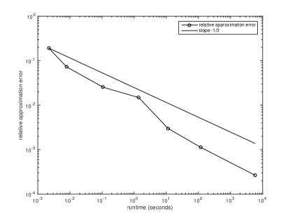
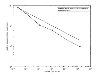
Figure 1: Empirical convergence of the scheme (11) for the recursive pricing with default risk example in Subsection 3.1. Left: Relative approximation errors $\scriptstyle{\frac{1}{10|\texttt{v}|}\sum_{i=1}^{10}|{\bf U}^{i,[1]}_{\rho,\rho}(0,x_{0})-\texttt{v}|}$ for $\rho\in\{1,2,\ldots,7\}$ against the average runtime in the case $d=1$. Right: Relative approximation increments $\scriptstyle{\left(\frac{1}{10}\sum_{i=1}^{10}|{\bf U}^{i,[1]}_{\rho+1,\rho+1}(0,x_{0})-{\bf U}^{i,[1]}_{\rho,\rho}(0,x_{0})|\right)\big{/}\left(\frac{1}{10}|\sum_{i=1}^{10}{\bf U}^{i,[1]}_{7,7}(0,x_{0})|\right)}$ for $\rho\in\{1,2,\ldots,6\}$ against the average runtime in the case $d=100$.

3.2 Pricing with counterparty credit risk

In this subsection we present a numerical simulation of a semilinear PDE that arises in the valuation of derivative contracts with counterparty credit risk. The PDE is a special case of the PDEs that are, e.g., derived in Henry-Labordère [53] and Burgard & Kjaer [13].

Throughout this subsection assume the setting in the beginning of Section 3, let $\bar{\sigma}=0.2$, $\beta=0.03$, $K_{1},L\in{\mathbbm{R}}$, $K_{2}\in(K_{1},\infty)$ and assume for all $s\in[0,T]$, $t\in[s,T]$, $x=(x_{1},\dots,x_{d})\in{\mathbbm{R}}^{d}$, $y\in{\mathbbm{R}}$, $z\in{\mathbbm{R}}^{d}$, $k\in{\mathbbm{N}}_{0}$, $\rho\in{\mathbbm{N}}$, $\theta\in\Theta$ that $T=2$, $\eta(x)=x$, $\mu(s,x)=0$, $\sigma(s,x)=\bar{\sigma}\operatorname{diag}(x)$, $x_{0}=100\cdot(1,1,\dots,1)\in{\mathbbm{R}}^{d}$, $\mathcal{D}_{x,s,t}^{k,\rho,\theta}=\exp(-\tfrac{\bar{\sigma}^{2}}{2}(t-s))\exp\!\left(\bar{\sigma}\operatorname{diag}(\Delta W^{\theta}_{s,t})\right)$, $\mathcal{X}^{k,\rho,\theta}_{x,s,t}=\mathcal{D}_{x,s,t}^{k,\rho,\theta}x$, $f(s,x,y,z)=\beta([y]^{+}-y)$, and

$$\begin{split}g(x)=\left[\min_{j\in\{1,2,\ldots,d\}}x_{j}-K_{1}\right]^{+}-\left[\min_{j\in\{1,2,\ldots,d\}}x_{j}-K_{2}\right]^{+}-L.\end{split}$$ (20)

Note that the solution $u$ of the PDE (13) satisfies for all $t\in[0,T)$, $x=(x_{1},x_{2},\ldots,x_{d})\in{\mathbbm{R}}^{d}$ that $u(T,x)=\min\{\max\{\min_{j\in\{1,2,\ldots,d\}}x_{j},K_{1}\},K_{2}\}-K_{1}-L$ and

$$\begin{split}&(\tfrac{\partial}{\partial t}u)(t,x)-\beta\min\{u(t,x),0\}+\tfrac{\bar{\sigma}^{2}}{2}\sum_{i=1}^{d}|x_{i}|^{2}\big{(}\tfrac{\partial^{2}}{\partial x^{2}_{i}}u\big{)}(t,x)=0.\end{split}$$ (21)

In (21) the function $u$ models the price of an European financial derivative with possibly negative payoff $g$ at maturity $T$ whose buyer may default. The number $u(t,x)\in{\mathbbm{R}}$ describes the price of the financial derivative at time $t\in[0,T]$ in dependence on the prices $x=(x_{1},\ldots,x_{d})\in{\mathbbm{R}}^{d}$ of the $d$ underlyings of the model given that no default has occurred before time $t$. In the model the default-payoff depends on the price of the derivative itself. The choice of the parameters is based on the choice of parameters in Henry-Labordère [53, Subsection 5.3]. In the case $d=1$ we choose that $K_{1}=90$, $K_{2}=110$, and $L=10$. In the case $d=100$ we choose that $K_{1}=30$, $K_{2}=60$, and $L=15$. Matlab code 13 presents the parameter values in the case $d=100$. In the case $d=1$ line 3 of Matlab code 13 is replaced by dim=1; and lines 7, 8, and 9 are changed to K1=90;, K2=110;, and L=10;, respectively. The simulation results are shown in Figure 2, the right-hand side of Figure 3, and Tables 3 and 4. Figure 2 suggests an empirical convergence rate close to $\nicefrac{{1}}{{3}}$.

⬇

1function [T,dim,f,g,eta,mu,sigma] = modelparameters()

2 T=2;

3 dim=100;

4 sigma=0.2;

5 mu=0;

6 beta=0.03;

7 K1=30;

8 K2=60;

9 L=15;

10 f = @(t,x,y,z) beta*(subplus(y)-y);

11 g = @(x) subplus(min(x,[],1)-K1)-subplus(min(x,[],1)-K2)-L;

12 eta=@(x) x;

13end

Matlab code 13: A Matlab function that returns the parameter values for the pricing with counterparty credit risk example.

$\rho$	1	2	3	4	5	6	7
average runtime in seconds	0.002	0.008	0.093	0.968	11.430	155.607	6226.101
$\overline{{\bf U}}^{[1]}_{\rho,\rho}(0,x_{0})=\frac{1}{10}\sum_{i=1}^{10}{\bf U}^{i,[1]}_{\rho,\rho}(0,x_{0})$	-0.582	-3.614	-0.767	-0.433	-0.916	-0.866	-0.884
$\sqrt{\frac{1}{9}\sum_{i=1}^{10}|{\bf U}^{i,[1]}_{\rho,\rho}(0,x_{0})-\overline{{\bf U}}^{[1]}_{\rho,\rho}(0,x_{0})|^{2}}$	9.346	3.964	1.279	0.782	0.105	0.067	0.015
$\frac{1}{10}\sum_{i=1}^{10}\frac{|{\bf U}^{i,[1]}_{\rho,\rho}(0,x_{0})-\texttt{v}|}{|\texttt{v}|}$	9.8923	4.1417	1.1794	0.7941	0.0943	0.0617	0.0135

Table 3: Average runtime, empirical mean, empirical standard deviation, and relative approximation error in the case $d=1$ for the pricing with counterparty credit risk example in Subsection 3.2. The approximation by the finite difference approximation scheme in Matlab code 6 yields $\texttt{v=approximateUfinitediffgbm(0,x0,2\^{}11)}\approx-0.883$.

$\rho$	1	2	3	4	5	6	7
average runtime in seconds	0.002	0.018	0.156	1.348	14.332	177.989	8935.848
$\overline{{\bf U}}^{[1]}_{\rho,\rho}(0,x_{0})=\frac{1}{10}\sum_{i=1}^{10}{\bf U}^{i,[1]}_{\rho,\rho}(0,x_{0})$	5.823	1.878	2.376	2.450	2.607	2.617	2.626
$\sqrt{\frac{1}{9}\sum_{i=1}^{10}|{\bf U}^{i,[1]}_{\rho,\rho}(0,x_{0})-\overline{{\bf U}}^{[1]}_{\rho,\rho}(0,x_{0})|^{2}}$	5.741	3.051	1.041	0.335	0.053	0.027	0.008
${\frac{1}{10}\sum_{i=1}^{10}\frac{|{\bf U}^{i,[1]}_{\rho+1,\rho+1}(0,x_{0})-{\bf U}^{i,[1]}_{\rho,\rho}(0,x_{0})|}{|\overline{{\bf U}}^{[1]}_{7,7}(0,x_{0})|}}$	1.7971	1.0354	0.2758	0.1004	0.0148	0.0094

Table 4: Average runtime, empirical mean, empirical standard deviation, and relative approximation increments in the case $d=100$ for the pricing with counterparty credit risk example in Subsection 3.2.

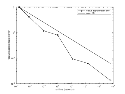
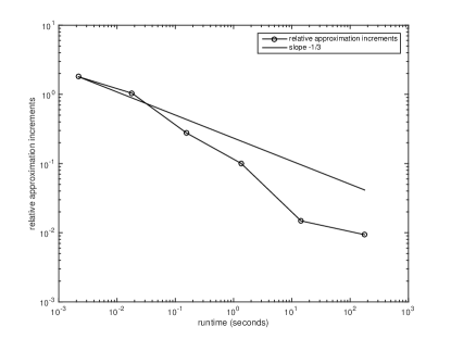
Figure 2: Empirical convergence of the scheme (11) for the pricing with counterparty credit risk example in Subsection 3.2. Left: Relative approximation errors $\scriptstyle{\frac{1}{10|\texttt{v}|}\sum_{i=1}^{10}|{\bf U}^{i,[1]}_{\rho,\rho}(0,x_{0})-\texttt{v}|}$ for $\rho\in\{1,2,\ldots,7\}$ against the average runtime in the case $d=1$. Right: Relative approximation increments $\scriptstyle{\left(\frac{1}{10}\sum_{i=1}^{10}|{\bf U}^{i,[1]}_{\rho+1,\rho+1}(0,x_{0})-{\bf U}^{i,[1]}_{\rho,\rho}(0,x_{0})|\right)\big{/}\left(\frac{1}{10}|\sum_{i=1}^{10}{\bf U}^{i,[1]}_{7,7}(0,x_{0})|\right)}$ for $\rho\in\{1,2,\ldots,6\}$ against the average runtime in the case $d=100$.

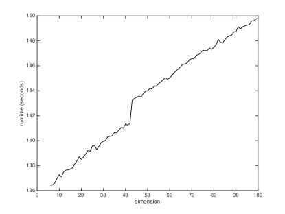
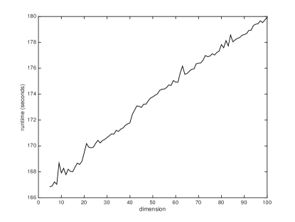
Figure 3: Left: Runtime needed to compute one realization of ${\bf U}^{1}_{6,6}(0,x_{0})$ against dimension $d\in\{5,6,\ldots,100\}$ for the recursive pricing with default risk example in Subsection 3.1. Right: Runtime needed to compute one realization of ${\bf U}^{1}_{6,6}(0,x_{0})$ against dimension $d\in\{5,6,\ldots,100\}$ for the pricing with counterparty credit risk example in Subsection 3.2.

3.3 Pricing with different interest rates for borrowing and lending

We consider a pricing problem of an European option in a financial market with different interest rates for borrowing and lending. The model goes back to Bergman [9] and serves as a standard example in the literature on numerical methods for BSDEs (see, e.g., [42, 7, 8, 12, 22]).

Throughout this subsection assume the setting in the beginning of Section 3, let $\bar{\mu}=0.06$, $\bar{\sigma}=0.2$, $R^{l}=0.04$, $R^{b}=0.06$, and assume for all $s\in[0,T]$, $t\in[s,T]$, $x=(x_{1},\dots,x_{d})\in{\mathbbm{R}}^{d}$, $y\in{\mathbbm{R}}$, $z=(z_{1},\dots,z_{d})\in{\mathbbm{R}}^{d}$, $k\in{\mathbbm{N}}_{0}$, $\rho\in{\mathbbm{N}}$, $\theta\in\Theta$ that $T=0.5$, $\eta(x)=x$, $\mu(s,x)=\bar{\mu}x$, $\sigma(s,x)=\bar{\sigma}\operatorname{diag}(x)$, $x_{0}=100\cdot(1,1,\dots,1)\in{\mathbbm{R}}^{d}$, $\mathcal{D}_{x,s,t}^{k,\rho,\theta}=\exp((\bar{\mu}-\tfrac{\bar{\sigma}^{2}}{2})(t-s))\exp\!\left(\bar{\sigma}\operatorname{diag}(\Delta W^{\theta}_{s,t})\right)$, $\mathcal{X}^{k,\rho,\theta}_{x,s,t}=\mathcal{D}_{x,s,t}^{k,\rho,\theta}x$, and

$$f(s,x,y,z)=-R^{l}y-\frac{(\bar{\mu}-R^{l})}{\bar{\sigma}}\left(\sum_{i=1}^{d}z_{i}\right)+(R^{b}-R^{l})\left[\frac{1}{\bar{\sigma}}\left(\sum_{i=1}^{d}z_{i}\right)-y\right]^{+}.$$ (22)

Note that the solution $u$ of the PDE (13) satisfies for all $t\in[0,T)$, $x=(x_{1},x_{2},\ldots,x_{d})\in{\mathbbm{R}}^{d}$ that $u(T,x)=g(x)$ and

$$(\tfrac{\partial}{\partial t}u)(t,x)+\tfrac{\bar{\sigma}^{2}}{2}\sum_{i=1}^{d}|x_{i}|^{2}\big{(}\tfrac{\partial^{2}}{\partial x^{2}_{i}}u\big{)}(t,x)\\ -\min\!\bigg{\{}R^{b}\bigg{(}u(t,x)-\sum_{i=1}^{d}x_{i}\big{(}\tfrac{\partial}{\partial x_{i}}u\big{)}(t,x)\bigg{)},R^{l}\bigg{(}u(t,x)-\sum_{i=1}^{d}x_{i}\big{(}\tfrac{\partial}{\partial x_{i}}u\big{)}(t,x)\bigg{)}\bigg{\}}=0.$$ (23)

In (23) the function $u$ models the price of an European financial derivative with payoff $g$ at maturity $T$ in a financial market with a higher interest rate for borrowing than for lending. The number $u(t,x)\in{\mathbbm{R}}$ describes the price of the financial derivative at time $t\in[0,T]$ in dependence on the prices $x=(x_{1},\ldots,x_{d})\in{\mathbbm{R}}^{d}$ of the $d$ underlyings of the model. In the case $d=1$, assume that for all $x\in{\mathbbm{R}}$ it holds that $g(x)=[x-100]^{+}$. This setting agrees with the setting in Gobet, Lemor, & Warin [42, Subsection 6.3.1], where it is also noted that the PDE (23) is actually linear. More precisely, $u$ also satisfies (13) for all $t\in[0,T)$, $x\in{\mathbbm{R}}$ with $f$ being replaced by $\bar{f}\colon[0,T]\times{\mathbbm{R}}\times{\mathbbm{R}}\times{\mathbbm{R}}\to{\mathbbm{R}}$ satisfying for all $t\in[0,T]$, $x,y,z\in{\mathbbm{R}}$ that $\bar{f}(t,x,y,z)=-R^{b}y-\frac{(\bar{\mu}-R^{b})}{\bar{\sigma}}z$. In the case $d=100$, assume that for all $x=(x_{1},\dots,x_{d})\in{\mathbbm{R}}^{d}$ it holds that $g(x)=[\max_{i\in\{1,\ldots,100\}}x_{i}-120]^{+}-2[\max_{i\in\{1,\ldots,100\}}x_{i}-150]^{+}$. This choice of $g$ is based on the choice of $g$ in Bender, Schweizer, & Zhuo [8, Subsection 4.2]. We note that with this choice of $g$ the PDE (23) can not be reduced to a linear PDE. Matlab code 14 presents the parameter values in the case $d=100$. In the case $d=1$ line 3 of Matlab code 14 is replaced by dim=1; and line 9 of Matlab code 14 is replaced by g=@(x) subplus(x-100);. The simulation results are shown in Figure 4, the left-hand side of Figure 6, and Tables 5 and 6. The left-hand side of Figure 4 suggests an empirical convergence rate close to $\nicefrac{{1}}{{3}}$ in the case $d=1$. Moreover, the right-hand side of Figure 4 suggests an empirical convergence rate close to $\nicefrac{{1}}{{4}}$ in the case $d=100$.

⬇

1function [T,dim,f,g,eta,mu,sigma] = modelparameters()

2 T = 0.5;

3 dim=100;

4 Rl=0.04;

5 Rb=0.06;

6 mu=0.06;

7 sigma=0.2;

8 f = @(t,x,y,z) -Rl.*y-(mu-Rl)/sigma*sum(z,1)+(Rb-Rl)*subplus(1/sigma*sum(z,1)-y);

9 g= @(x) subplus(max(x,[],1)-120)-2*subplus(max(x,[],1)-150);

10 eta=@(x) x;

11end

Matlab code 14: A Matlab function that returns the parameter values for the pricing with different interest rates example.

$\rho$	1	2	3	4	5	6	7
average runtime in seconds	0.001	0.011	0.114	0.990	11.347	132.484	6264.475
$\overline{{\bf U}}^{[1]}_{\rho,\rho}(0,x_{0})=\frac{1}{10}\sum_{i=1}^{10}{\bf U}^{i,[1]}_{\rho,\rho}(0,x_{0})$	5.695	5.947	7.085	7.631	7.156	7.162	7.166
$\sqrt{\frac{1}{9}\sum_{i=1}^{10}|{\bf U}^{i,[1]}_{\rho,\rho}(0,x_{0})-\overline{{\bf U}}^{[1]}_{\rho,\rho}(0,x_{0})|^{2}}$	7.780	4.080	1.612	0.811	0.151	0.071	0.016
$\frac{1}{10}\sum_{i=1}^{10}\frac{|{\bf U}^{i,[1]}_{\rho,\rho}(0,x_{0})-\texttt{v}|}{|\texttt{v}|}$	0.8285	0.4417	0.1777	0.1047	0.0170	0.0086	0.0019

Table 5: Average runtime, empirical mean, empirical standard deviation, and relative approximation error in the case $d=1$ for the pricing with different interest rates example in Subsection 3.3. The approximation by the finite difference approximation scheme in Matlab code 6 yields $\texttt{v=approximateUfinitediffgbm(0,x0,2\^{}11)}\approx 7.156$.

$\rho$	1	2	3	4	5	6	7
average runtime in seconds	0.011	0.015	0.151	1.317	14.813	181.647	8825.390
$\overline{{\bf U}}^{[1]}_{\rho,\rho}(0,x_{0})=\frac{1}{10}\sum_{i=1}^{10}{\bf U}^{i,[1]}_{\rho,\rho}(0,x_{0})$	28.902	22.854	23.356	21.771	21.374	21.274	21.299
$\sqrt{\frac{1}{9}\sum_{i=1}^{10}|{\bf U}^{i,[1]}_{\rho,\rho}(0,x_{0})-\overline{{\bf U}}^{[1]}_{\rho,\rho}(0,x_{0})|^{2}}$	8.798	11.317	4.492	2.953	1.449	1.376	0.467
${\frac{1}{10}\sum_{i=1}^{10}\frac{|{\bf U}^{i,[1]}_{\rho+1,\rho+1}(0,x_{0})-{\bf U}^{i,[1]}_{\rho,\rho}(0,x_{0})|}{|\overline{{\bf U}}^{[1]}_{7,7}(0,x_{0})|}}$	0.6446	0.4770	0.1840	0.1190	0.0844	0.0467

Table 6: Average runtime, empirical mean, empirical standard deviation, and relative approximation increments in the case $d=100$ for the pricing with different interest rates example in Subsection 3.3.

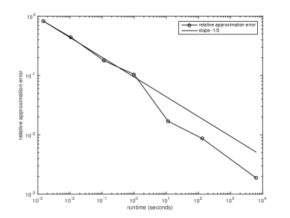
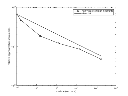
Figure 4: Empirical convergence of the scheme (11) for the pricing with different interest rates example in Subsection 3.3. Left: Relative approximation errors $\scriptstyle{\frac{1}{10|\texttt{v}|}\sum_{i=1}^{10}|{\bf U}^{i,[1]}_{\rho,\rho}(0,x_{0})-\texttt{v}|}$ for $\rho\in\{1,2,\ldots,7\}$ against the average runtime in the case $d=1$. Right: Relative approximation increments $\scriptstyle{\left(\frac{1}{10}\sum_{i=1}^{10}|{\bf U}^{i,[1]}_{\rho+1,\rho+1}(0,x_{0})-{\bf U}^{i,[1]}_{\rho,\rho}(0,x_{0})|\right)\big{/}\left(\frac{1}{10}|\sum_{i=1}^{10}{\bf U}^{i,[1]}_{7,7}(0,x_{0})|\right)}$ for $\rho\in\{1,2,\ldots,6\}$ against the average runtime in the case $d=100$.

3.4 Allen-Cahn equation

In this subsection we consider the Allen-Cahn equation with a double well potential.

Throughout this subsection assume the setting in the beginning of Section 3 and assume for all $s\in[0,T]$, $t\in[s,T]$, $x=(x_{1},\dots,x_{d})\in{\mathbbm{R}}^{d}$, $y\in{\mathbbm{R}}$, $z\in{\mathbbm{R}}^{d}$, $k\in{\mathbbm{N}}_{0}$, $\rho\in{\mathbbm{N}}$, $\theta\in\Theta$ that $T=1$, $\eta(x)=x$, $\mu(s,x)=0$, $\sigma(s,x)=\operatorname{I}_{{\mathbbm{R}}^{d\times d}}$, $x_{0}=(0,0,\dots,0)\in{\mathbbm{R}}^{d}$, $\mathcal{X}^{k,\rho,\theta}_{x,s,t}=x+W^{\theta}_{t}-W^{\theta}_{s}$, $\mathcal{D}^{k,\rho,\theta}_{x,s,t}=\operatorname{I}_{{\mathbbm{R}}^{d\times d}}$, $f(s,x,y,z)=y-y^{3}$, and $g(x)=\frac{1}{1+\max\{|x_{1}|^{2},...,|x_{d}|^{2}\}}$. Note that the solution $u$ of the PDE (13) satisfies for all $t\in[0,T)$, $x\in{\mathbbm{R}}^{d}$ that $u(T,x)=\frac{1}{1+\max\{|x_{1}|^{2},...,|x_{d}|^{2}\}}$ and

$$\begin{split}&(\tfrac{\partial}{\partial t}u)(t,x)+u(t,x)-\big{[}u(t,x)\big{]}^{3}+\tfrac{1}{2}\big{(}\Delta_{x}u\big{)}(t,x)=0.\end{split}$$ (24)

Matlab code 15 presents the parameter values in the case $d=100$. In the case $d=1$ line 3 of Matlab code 15 is replaced by dim=1;. The simulation results are shown in Figure 5, the right-hand side of Figure 6, and Tables 7 and 8. The left-hand side of Figure 5 suggests an empirical convergence rate close to $\nicefrac{{1}}{{4}}$ in the case $d=1$. Moreover, the right-hand side of Figure 5 suggests an empirical convergence rate close $\nicefrac{{1}}{{3}}$ in the case $d=100$.

⬇

1function [T,dim,f,g,eta,mu,sigma] = modelparameters()

2 T = 1;

3 dim=100;

4 mu=0;

5 sigma=1;

6 f = @(t,x,y,z) y-y.^3;

7 g = @(x) 1./(1+max(x.^2,[],1));

8 eta=@(x) x;

9end

Matlab code 15: A Matlab function that returns the parameter values for the Allen-Cahn example.

$\rho$	1	2	3	4	5
average runtime in seconds	0.005	0.035	0.237	7.402	345.124
$\overline{{\bf U}}^{[1]}_{\rho,\rho}(0,x_{0})=\frac{1}{10}\sum_{i=1}^{10}{\bf U}^{i,[1]}_{\rho,\rho}(0,x_{0})$	1.027	0.866	0.918	0.894	0.897
$\sqrt{\frac{1}{9}\sum_{i=1}^{10}|{\bf U}^{i,[1]}_{\rho,\rho}(0,x_{0})-\overline{{\bf U}}^{[1]}_{\rho,\rho}(0,x_{0})|^{2}}$	0.219	0.131	0.078	0.037	0.013
$\frac{1}{10}\sum_{i=1}^{10}\frac{|{\bf U}^{i,[1]}_{\rho,\rho}(0,x_{0})-\texttt{v}|}{|\texttt{v}|}$	0.2462	0.1197	0.0691	0.0302	0.0124

Table 7: Average runtime, empirical mean, empirical standard deviation, and relative approximation error in the case $d=1$ for the Allen-Cahn equation in Subsection 3.4. The approximation by the finite difference approximation scheme in Matlab code 7 yields $\texttt{v=approximateUfinitediffgbm(0,x0,2\^{}11)}\approx 0.905$.

$\rho$	1	2	3	4	5
average runtime in seconds	0.002	0.043	0.280	9.687	453.418
$\overline{{\bf U}}^{[1]}_{\rho,\rho}(0,x_{0})=\frac{1}{10}\sum_{i=1}^{10}{\bf U}^{i,[1]}_{\rho,\rho}(0,x_{0})$	0.246	0.284	0.313	0.319	0.317
$\sqrt{\frac{1}{9}\sum_{i=1}^{10}|{\bf U}^{i,[1]}_{\rho,\rho}(0,x_{0})-\overline{{\bf U}}^{[1]}_{\rho,\rho}(0,x_{0})|^{2}}$	0.043	0.013	0.007	0.004	0.002
${\frac{1}{10}\sum_{i=1}^{10}\frac{|{\bf U}^{i,[1]}_{\rho+1,\rho+1}(0,x_{0})-{\bf U}^{i,[1]}_{\rho,\rho}(0,x_{0})|}{|\overline{{\bf U}}^{[1]}_{5,5}(0,x_{0})|}}$	0.1484	0.0909	0.0254	0.0102

Table 8: Average runtime, empirical mean, empirical standard deviation, and relative approximation increments in the case $d=100$ for the Allen-Cahn equation in Subsection 3.4.

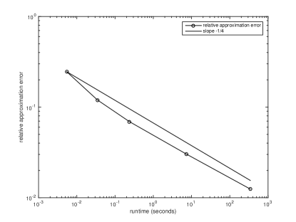
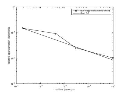
Figure 5: Empirical convergence of the scheme (10) for the Allen-Cahn equation in Subsection 3.4. Left: Relative approximation errors $\scriptstyle{\frac{1}{10|\texttt{v}|}\sum_{i=1}^{10}|{\bf U}^{i,[1]}_{\rho,\rho}(0,x_{0})-\texttt{v}|}$ for $\rho\in\{1,2,\ldots,5\}$ against the average runtime in the case $d=1$. Right: Relative approximation increments $\scriptstyle{\left(\frac{1}{10}\sum_{i=1}^{10}|{\bf U}^{i,[1]}_{\rho+1,\rho+1}(0,x_{0})-{\bf U}^{i,[1]}_{\rho,\rho}(0,x_{0})|\right)\big{/}\left(\frac{1}{10}|\sum_{i=1}^{10}{\bf U}^{i,[1]}_{5,5}(0,x_{0})|\right)}$ for $\rho\in\{1,2,3,4\}$ against the average runtime in the case $d=100$.

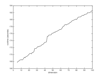
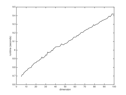
Figure 6: Left: Runtime needed to compute one realization of ${\bf U}^{1}_{6,6}(0,x_{0})$ against dimension $d\in\{5,6,\ldots,100\}$ for the pricing with different interest rates example in Subsection 3.3. Right: Average runtime needed to compute 20 realizations of ${\bf U}^{1}_{4,4}(0,x_{0})$ against dimension $d\in\{5,6,\ldots,100\}$ for the Allen-Cahn equation in Subsection 3.4.

3.5 An example with an explicit solution

In this subsection we discuss an example with an explicit solution whose three-dimensional version has been considered in Chassagneux [15].

Throughout this subsection assume the setting in the beginning of Section 3, let $\bar{\sigma}=0.25$, and assume for all $s\in[0,T]$, $t\in[s,T]$, $x=(x_{1},\dots,x_{d})\in{\mathbbm{R}}^{d}$, $y\in{\mathbbm{R}}$, $z=(z_{1},\ldots,z_{d})\in{\mathbbm{R}}^{d}$, $k\in{\mathbbm{N}}_{0}$, $\rho\in{\mathbbm{N}}$, $\theta\in\Theta$ that $T=0.5$, $d=100$, $\eta(x)=x$, $\mu(s,x)=0$, $\sigma(s,x)=\bar{\sigma}\operatorname{I}_{{\mathbbm{R}}^{d\times d}}$, $x_{0}=(0,0,\dots,0)\in{\mathbbm{R}}^{d}$, $\mathcal{X}^{k,\rho,\theta}_{x,s,t}=x+W^{\theta}_{t}-W^{\theta}_{s}$, $\mathcal{D}^{k,\rho,\theta}_{x,s,t}=\operatorname{I}_{{\mathbbm{R}}^{d\times d}}$, $f(s,x,y,z)=\bar{\sigma}\big{(}y-\frac{2+\bar{\sigma}^{2}d}{2\bar{\sigma}^{2}d}\big{)}\big{(}\sum_{i=1}^{d}z_{i}\big{)}$, and $g(x)=\frac{\exp(T+\sum_{i=1}^{d}x_{i})}{1+\exp(T+\sum_{i=1}^{d}x_{i})}$. Note that the solution $u$ of the PDE (13) satisfies for all $t\in[0,T)$, $x=(x_{1},x_{2},\ldots,x_{d})\in{\mathbbm{R}}^{d}$ that $u(T,x)=\frac{\exp(T+\sum_{i=1}^{d}x_{i})}{1+\exp(T+\sum_{i=1}^{d}x_{i})}$ and

$$\begin{split}&(\tfrac{\partial}{\partial t}u)(t,x)+\left[\bar{\sigma}^{2}u(t,x)-\tfrac{1}{d}-\tfrac{\bar{\sigma}^{2}}{2}\right]\bigg{[}\sum_{i=1}^{d}(\tfrac{\partial}{\partial x_{i}}u)(t,x)\bigg{]}+\tfrac{\bar{\sigma}^{2}}{2}\big{(}\Delta_{x}u\big{)}(t,x)=0.\end{split}$$ (25)

Next we observe that $u$ satisfies for all $s\in[0,T]$, $x=(x_{1},\dots,x_{d})\in{\mathbbm{R}}^{d}$ that

$$u(s,x)=\frac{\exp(s+\sum_{i=1}^{d}x_{i})}{1+\exp(s+\sum_{i=1}^{d}x_{i})}.$$ (26)

Matlab code 16 presents the parameter values. The simulation results are shown in Figure 7 and Table 9. The left-hand side of Figure 7 suggests an empirical convergence rate close to $\nicefrac{{1}}{{4}}$.

⬇

1function [T,dim,f,g,eta,mu,sigma] = modelparameters()

2 T = 0.5;

3 dim=100;

4 mu=0;

5 sigma=0.25;

6 f = @(t,x,y,z) sigma*(y-(2+sigma^2*dim)/(2*sigma^2*dim)).*sum(z,1);

7 g = @(x) 1-1./(1+exp(T+sum(x,1)));

8 eta=@(x) x;

9end

Matlab code 16: A Matlab function that returns the parameter values for the Allen-Cahn example.

$\rho$	1	2	3	4	5
average runtime in seconds	0.002	0.021	0.352	11.677	545.871
$\overline{{\bf U}}^{[1]}_{\rho,\rho}(0,x_{0})=\frac{1}{10}\sum_{i=1}^{10}{\bf U}^{i,[1]}_{\rho,\rho}(0,x_{0})$	0.751	0.522	0.523	0.520	0.495
$\sqrt{\frac{1}{9}\sum_{i=1}^{10}|{\bf U}^{i,[1]}_{\rho,\rho}(0,x_{0})-\overline{{\bf U}}^{[1]}_{\rho,\rho}(0,x_{0})|^{2}}$	0.477	0.248	0.070	0.040	0.018
$\frac{1}{10}\sum_{i=1}^{10}\frac{|{\bf U}^{i,[1]}_{\rho,\rho}(0,x_{0})-\texttt{v}|}{|\texttt{v}|}$	0.9449	0.3931	0.1135	0.0767	0.0309

Table 9: Average runtime, empirical mean, empirical standard deviation, and relative approximation error in the case $d=100$ for the example PDE of Subsection 3.5. The exact value of the solution is $\texttt{v}=u(0,0)=0.5$.

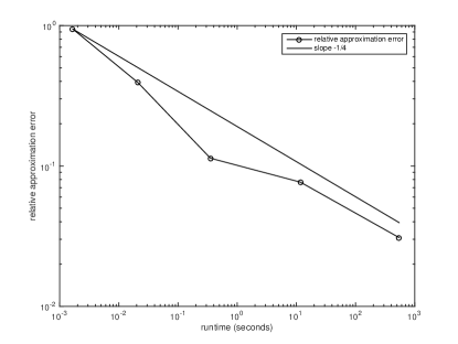
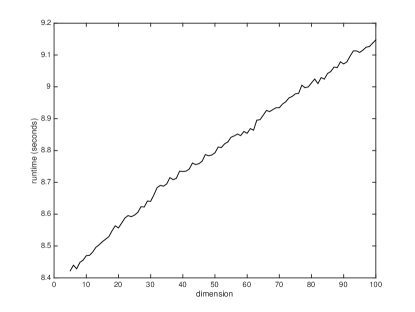
Figure 7: Performance of the scheme (10) for the example PDE of Subsection 3.5. Left: Relative approximation errors $\scriptstyle{\frac{1}{10|\texttt{v}|}\sum_{i=1}^{10}|{\bf U}^{i,[1]}_{\rho,\rho}(0,x_{0})-\texttt{v}|}$ for $\rho\in\{1,2,\ldots,5\}$ against the average runtime for the case $d=100$. Right: Average runtime needed to compute 20 realizations of ${\bf U}^{1}_{4,4}(0,x_{0})$ against dimension $d\in\{5,6,\ldots,100\}$.

4 Discussion of approximation methods from the literature

Deterministic methods for second-order parabolic PDEs are known to have exponentially growing computational effort. Since a program with $10^{80}$, say, floating point operations will never terminate (on a non-quantum computer), deterministic methods such as finite elements methods, finite difference methods, spectral Galerkin approximation methods, or sparse grid methods are not suitable for solving high-dimensional nonlinear second-order parabolic PDEs no matter what the convergence rate of the method is. For this reason we discuss only stochastic approximation methods for nonlinear second-order parabolic PDEs. In the literature we have found the following articles [11, 67, 4, 3, 10, 83, 42, 62, 26, 7, 41, 21, 24, 40, 22, 12, 16, 15, 23, 63, 81, 75, 76, 45, 44, 53, 55, 54, 37, 14, 60] which propose (possibly non-implementable) stochastic approximation methods for nonlinear second-order parabolic PDEs. All of these methods except for [53, 55, 54, 14, 60] exploit a stochastic representation with BSDEs due to Pardoux & Peng [70]. Moreover, all of these methods except for [40, 12, 37, 53, 55, 54, 14, 60] can be described in two steps. In the first step, time in the corresponding BSDE is discretized backwards in time via an explicit or an implicit Euler-type method which was investigated in detail, e.g., in Bouchard & Touzi [10] and Zhang [83]. The resulting approximations involve nested conditional expectations and, therefore, are not implementable. In the second step, these conditional expectations are approximated by ’straight-forward’ Monte Carlo simulations, by the quantization tree method (proposed in [4]), by a regression method based on kernel-estimation or on Malliavin calculus (proposed in [10]), by projections on function spaces (proposed in [42]), or by the cubature method on Wiener space (developed in [66] and proposed in [22]). The first step does not cause problems in high dimensions in the sense that the backward (explicit or implicit) Euler-type approximations converge under suitable assumptions with rate at least $0.5$ (see Theorem 5.3 in Zhang [83] and Theorem 3.1 in Bouchard & Touzi [10] for the backward implicit Euler-type method) and the computational effort (assuming the conditional expectations are known exactly) grows at most linearly in the dimension for fixed accuracy. For this reason, we discuss below in detail only the different methods for discretizing conditional expectations. In addition, we discuss the Wiener chaos decomposition method proposed in [12], the branching diffusion method proposed in [53], and methods based on density estimation proposed in [14, 60].

A difficulty in our discussion below is that the discussed algorithms (except for the branching diffusion method) depend on different parameters and the optimal choice of these parameters is unknown since no lower estimates for the approximation errors are known. For this reason we will choose parameters which are optimal with respect to the best known upper error bound. For these parameter choices we will show below for the discussed algorithms (except for the branching diffusion method) that the computational effort fails to grow at most polynomially both in the dimension and in the reciprocal of the best known upper error bound.

Throughout this section assume the setting in Subsection 2.3, let $u^{\infty}\in C^{1,2}([0,T]\times{\mathbbm{R}}^{d},{\mathbbm{R}})$ be a function which satisfies (13) and we denote by $Y\colon[0,T]\times\Omega\to{\mathbbm{R}}$ the stochastic process which satisfies for all $t\in[0,T]$ that $Y_{t}=u^{\infty}(t,W_{t}^{0})$.

4.1 The ’straight-forward’ Monte Carlo method

The ’straight-forward’ Monte Carlo method approximates the conditional expectations involved in backward Euler-type approximations by Monte Carlo simulations. The resulting nesting of Monte Carlo averages is computational expensive in the following sense. If for a set $\pi\subseteq[0,T]$ with $|\pi|\in{\mathbbm{N}}$ many points and for $M\in{\mathbbm{N}}$ the random variable $Y^{\pi,M}\colon\Omega\to{\mathbbm{R}}$ is the ’straight-forward’ Monte Carlo approximation of $Y$ with time grid $\pi$ and $M$ Monte Carlo averages for each involved conditional expectation, then the number of realizations of scalar standard normal random variables required to compute $Y^{\pi,M}$ is $(Md)^{|\pi|}$ and the $L^{2}$-error satisfies for a suitable constant $c\in{\mathbbm{R}}$ independent of $\pi$ and $N$ that

$$\max_{t\in\pi}\|Y_{t}-Y^{\pi,M}_{t}\|_{L^{2}({\mathbb{P}};{\mathbbm{R}})}\leq c\left(|\pi|^{-\frac{1}{2}}+|\pi|M^{-1/2}\right),$$ (27)

see, e.g., Theorem 4.3 and Display (4.14) in Crisan & Manolarakis [21]. Thus the computational effort $(Md)^{(\frac{1}{|\pi|^{-1/2}})^{2}}\geq(Md)^{(\frac{c}{c|\pi|^{-1/2}+c|\pi|M^{-1/2}})^{2}}$ grows at least exponentially in the reciprocal of the right-hand side of (27). This suggests an at most logarithmic convergence rate of the ’straight-forward’ Monte Carlo method. We are not aware of a statement in the literature claiming that the ’straight-forward’ Monte Carlo method has a polynomial convergence rate.

4.2 The quantization tree method

The quantization tree method has been introduced in Bally & Pagès [4, 3]. In the proposed algorithm, time is discretized by the explicit backward Euler-type method. Moreover, one chooses a space-time grid and computes the transition probabilities for the underlying forward diffusion projected to this grid by Monte Carlo simulation. With these discrete-space transition probabilities one can then approximate all involved conditional expectations. If for a set $\pi\subseteq[0,T]$ with $|\pi|\in{\mathbbm{N}}$ many points and for $N\in{\mathbbm{N}}$ the random variable $Y^{\pi,N}\colon\Omega\to{\mathbbm{R}}$ is the quantization tree approximation of $Y$ with time grid $\pi$, a specific space grid with a total number of $N$ nodes and explicitly known transition probabilities of the forward diffusion and if the coefficients are sufficiently regular, then the number of realizations of scalar standard normal random variables required to compute $Y^{\pi,N}$ is at least $Nd|\pi|$ and Display (6) in Bally & Pagès [3] shows for optimal grids and a constant $c\in{\mathbbm{R}}$ independent of $\pi$ and $N$ that

$$\max_{t\in\pi}\|Y_{t}-Y^{\pi,N}_{t}\|_{L^{2}({\mathbb{P}};{\mathbbm{R}})}\leq c\left(\frac{1}{|\pi|}+\frac{|\pi|^{1+1/d}}{N^{1/d}}\right).$$ (28)

To ensure that this upper bound does not explode as $|\pi|\to\infty$ it is thus necessary to choose a space-time grid with at least $N=|\pi|^{d+1}$ many nodes when there are $|\pi|\in{\mathbbm{N}}$ many time steps. With this choice the computational effort of this algorithm grows exponentially fast in the dimension. We have not found a statement in the literature on the quantization tree method claiming that there exists a choice of parameters such that the computational effort grows at most polynomially both in the dimension and in the reciprocal of the prescribed accuracy.

4.3 The Malliavin calculus based regression method

The Malliavin calculus based regression method has been introduced in Section 6 in Bouchard & Touzi [10] and is based on the implicit backward Euler-type method. The algorithm involves iterated Skorohod integrals which by Display (3.2) in Crisan, Manolarakis, & Touzi [24] can be numerically computed with $2^{d}$ many independent standard normally distributed random variables. In that case the computational effort grows exponentially fast in the dimension. We are not aware of an approximation method of the involved iterated Skorohod integrals whose computational effort does not grow exponentially fast in the dimension. Example 4.1 in Bouchard & Touzi [10] also mentions a method for approximating all involved conditional expectations using kernel estimation. For this method we have not found an upper error estimate in the literature so that we do not known how to choose the bandwidth matrix of the kernel estimation given the number of time grid points.

4.4 The projection on function spaces method

The projection on function spaces method has been proposed in Gobet, Lemor, & Warin [42]. The algorithm is based on estimating the involved conditional expectations by considering the projections of the random variables on a finite-dimensional function space and then estimating these projections by Monte Carlo simulation. In general the projection error and the computational effort depend on the choice of the basis functions. In the literature we have found the following two choices of basis functions. In Gobet, Lemor, & Warin [42] (see also Gobet & Lemor [41] and Lemor, Gobet, & Warin [62]) indicator functions of hypercubes are employed as basis functions. In this case there exists $c\in{\mathbbm{R}}$ such that a projection error ${\varepsilon}\in(0,\infty)$ can be achieved by simulating $\lfloor c{\varepsilon}^{-(3+2d)}|\log({\varepsilon})|\rfloor$ paths of the forward diffusion. With this choice, the computational effort of the algorithm grows exponentially fast in the dimension for fixed accuracy ${\varepsilon}\in(0,1)$. Ruijter & Oosterlee [75] use certain cosine functions as basis functions and motivate this with a Fourier cosine series expansion. The resulting approximation method has only been specified in a one-dimensional setting so that the computational effort in a high-dimensional setting remained unclear. We have not found a statement in the literature on the projection on function spaces method claiming that there exists a choice of function spaces and other algorithm parameters such that the computational effort of the method grows at most polynomially both in the dimension of the PDE and in the reciprocal of the prescribed accuracy.

4.5 The cubature on Wiener space method

The cubature on Wiener space method for approximating solutions of PDEs has been introduced in Crisan & Manolarakis [22]. This method combines the implicit backward Euler-type scheme with the cubature method developed in Lyons & Victoir [66] for constructing finitely supported measures that approximate the distribution of the solution of a stochastic differential equation. This method has a parameter $m\in{\mathbbm{N}}$ and constructs for every finite time grid $\pi\subseteq[0,T]$ (with $|\pi|\in{\mathbbm{N}}$ points) a sequence $w_{1},\ldots,w_{(N_{m,d})^{|\pi|}}\in C^{0}([0,1],{\mathbbm{R}}^{d})$ of paths with bounded variation where $N_{m,d}\in{\mathbbm{N}}$ is the number of nodes needed for a cubature formula of degree $m$ with respect to the $d$-dimensional Gaussian measure. We note that this construction is independent of $f$ and $g$ and can be computed once and then tabularized. Using these paths, Corollary 4.2 in Crisan & Manolarakis [22] shows in the case $m\geq 3$ that there exists a constant $c\in[0,\infty)$, a sequence $\pi_{n}\subseteq[0,T]$, $n\in{\mathbbm{N}}$, of finite time grids and there exist implementable approximations $Y^{n}\colon\pi_{n}\times\Omega\to{\mathbbm{R}}$, $n\in{\mathbbm{N}}$, of the exact solution $Y$ such that for all $n\in{\mathbbm{N}}$ it holds that $0\in\pi_{n}$, $\pi_{n}$ has $n+1$ elements and

$$\|Y_{0}-Y^{\pi_{n}}_{0}\|_{L^{2}({\mathbb{P}};{\mathbbm{R}})}\leq\tfrac{c}{n}.$$ (29)

In this form of the algorithm, the computational effort for calculating $Y^{\pi_{n}}$, which is at least the number $(N_{m,d})^{n}$ of paths to be used, grows exponentially in the reciprocal of the right-hand side of (29). To avoid this exponential growth of the computational effort in the number of cubature paths, Crisan & Manolarakis [22] specify two methods (a tree based branching algorithm of Crisan & Lyons [20] and the recombination method of Litterer & Lyons [64]) which reduce the number of nodes and which result in approximations which converge with polynomial rate; cf. Theorem 5.4 in[22]. The constant in the upper error estimate in Theorem 5.4 in [22] may depend on the dimension (cf. also (5.16) and the proof of Lemma 3.1 in [22]). Simulations in the literature on the cubature method were performed in dimension 1 (see Figures 1–4 in [22] and Figure 1 in [23]) or dimension 5 (see Figures 5–6 in [22]). To the best of our knowledge, there exist no statement in the literature on the cubature method which asserts that the computational effort of the cubature method together with a suitable complexity reduction method grows at most polynomially both in the dimension of the PDE and in the reciprocal of the prescribed accuracy.

4.6 The Wiener chaos decomposition method

The Wiener chaos decomposition method has been introduced in Briand & Labart [12] and has been extended to the case of BSDEs with jumps in Geiss & Labart [37]. The algorithm is based on Picard iterations of the associated BSDE and evaluates the involved nested conditional expectations using Wiener chaos decomposition formulas. This algorithm does not need to discretize time since Wiener integrals over integrands with explicitly known antiderivative can be simulated exactly. The computational complexity of approximating the solution of a BSDE of dimension $d$ using a Wiener chaos decomposition of order $p\in{\mathbbm{N}}$, $K\in{\mathbbm{N}}$ Picard iterations, $M\in{\mathbbm{N}}$ Monte Carlo samples for each conditional expectation, and $N\in{\mathbbm{N}}$ many time steps is of order $O(K\times M\times p\times(N\times d)^{p+1})$; see Section 3.2.2 in Briand & Labart [12]. To ensure that the approximation error converges to $0$ requires the order $p$ of the chaos decomposition to increase to $\infty$. This implies that the computational effort fails to grow at most polynomially both in the dimension of the PDE and in the reciprocal of the prescribed accuracy. We also mention that we are not aware of a result in the literature that establishes a polynomial rate of convergence for the Wiener chaos decomposition method (see, e.g., Remark 4.8 in Briand & Labart [12]).

4.7 The branching diffusion method

The branching diffusion method has been proposed in Henry-Labordère [53]; see also the extensions to the non-Markovian case in [55] and to nonlinearities depending on derivatives in [54]. This method approximates the nonlinearity $f$ by polynomials and then exploits that the solution of a semilinear PDE with polynomial nonlinearity (KPP-type equations) can be represented as an expectation of a functional of a branching diffusion process due to Skorohod [77]. This expectation can then be numerically approximated with the standard Monte Carlo method and pathwise approximations of the branching diffusion process. The branching diffusion method does not suffer from the ’curse of dimensionality by construction’ and works in all dimensions. It’s convergence rate is $0.5$ if the forward diffusion can be simulated exactly and, in general, its rate is $0.5-$ using a pathwise approximation of the forward diffusion and the multilevel Monte Carlo method proposed in Giles [38].

The major drawback of the branching diffusion method is its insufficient applicability. This method replaces potentially ’nice’ nonlinearities by potentially ’non-nice’ polynomials. Semilinear PDEs with certain polynomial nonlinearities, however, can ’blow up’ in finite time; see, e.g., Fujita [34], Escobedo & Herrero [31] for analytical proofs and, e.g., Nagasawa & Sirao [69] and Lopez-Mimbela & Wakolbinger [65] for probabilistic proofs. If the approximating polynomial nonlinearity, the time horizon, and the terminal condition satisfy a certain condition, then the PDE does not ’blow up’ until time $T$ and the branching diffusion method is known to work well. More specifically, if there exist $\beta\in(0,\infty)$ and functions $(a_{k})_{k\in{\mathbbm{N}}_{0}}\colon[0,T]\times{\mathbbm{R}}^{d}\to{\mathbbm{R}}$ such that for all $(t,x,y,z)\in[0,T]\times{\mathbbm{R}}^{d}\times{\mathbbm{R}}\times{\mathbbm{R}}^{d}$ it holds that $f(t,x,y,z)=\beta\sum_{k=0}^{\infty}a_{k}(t,x)y^{k}-\beta y$, if the functions $\mu$ and $\sigma$ are bounded, continuous and Lipschitz in the second argument, and if $\forall x\in{\mathbbm{R}}^{d}\colon\eta(x)=x$, then Theorem 2.13 in [55] (see also Proposition 4.2 in [53] or Theorem 3.12 in [54]) shows that a sufficient condition for a stochastic representation with a branching diffusion to hold is that

$$\begin{split}\int_{\sup_{x\in{\mathbbm{R}}^{d}}|g(x)|}^{\infty}\tfrac{1}{\beta\max\left\{0,\sum_{k=0}^{\infty}\sup_{(t,x)\in[0,T]\times{\mathbbm{R}}^{d}}|a_{k}(t,x)|y^{k}-y\right\}}\,dy>T.\end{split}$$ (30)

For the branching diffusion method to converge with rate $0.5$ the random variables in the stochastic representation need to have finite second moments which leads to a more restrictive condition than (30); see Remark 2.14 in [55]. However, condition (30) is also necessary for the stochastic representation in [55] to hold if the functions $g$ and $(a_{k})_{k\in{\mathbbm{N}}_{0}}$ are constant and positive and if $\mu$ and $\sigma$ are constant (then the PDE (13) reduces to an ODE for which the ’blow-up’-behavior is well-known); see, e.g., Lemma 2.5 in [55].

The branching diffusion method also seems to have problems with polynomial nonlinearities where the exact solution does not ’blow up’ in finite time. Since no theoretical results are available in this direction, we illustrate this with simulations for an Allen-Cahn equation (a simplified version of the Ginzburg-Landau equation). More precisely, for the rest of this subsection assume that $T$, $\mu$, $\sigma$, $f$, and $g$ satisfy for all $(t,x,y,z)\in[0,T]\times{\mathbbm{R}}^{d}\times{\mathbbm{R}}\times{\mathbbm{R}}^{d}$ that $T=1$, $\mu(x)=\mu(0)$, $\sigma(x)=\sigma(0)$, $f(t,x,y,z)=y-y^{3}$, $g(x)=g(0)$, and $g(0)\geq 0$. Then (13) is an ODE and the solution $u^{\infty}$ satisfies for all $(t,x)\in[0,T]\times{\mathbbm{R}}^{d}$ that $u^{\infty}(t,x)=\left(1-(1-(g(0))^{-2})e^{2t-2}\right)^{-\frac{1}{2}}$. In this situation the sufficient condition (30) (choose for all $(t,x)\in[0,T]\times{\mathbbm{R}}^{d}$ and $k\in{\mathbbm{N}}_{0}\setminus\{1,3\}$ that $\beta=1$, $a_{1}(t,x)=2$, $a_{3}(t,x)=-1$, and $a_{k}(t,x)=0$) from Theorem 2.13 in [55] is equivalent to

$$\begin{split}1<\int_{|g(0)|}^{\infty}\tfrac{1}{y+y^{3}}\,dy=\left[\log(y)-\tfrac{1}{2}\log(1+y^{2})\right]_{|g(0)|}^{\infty}=\tfrac{1}{2}\log\left(1+\tfrac{1}{|g(0)|^{2}}\right)\end{split}$$ (31)

which is equivalent to $|g(0)|<(e^{2}-1)^{-\frac{1}{2}}=0.395623\ldots$ We simulated the branching diffusion approximations of $u^{\infty}(0,0)$ for different values of $g(0)$. Each approximation is an average over $M=10^{5}$ independent copies $(\Psi_{0,0}^{i})_{i\in\{1,2,\ldots,10^{5}\}}$ of the random variable $\Psi_{0,0}$ defined in (2.12) in Henry-Labordère, Tan, & Touzi [55] where we choose for all $k\in{\mathbbm{N}}_{0}$ that $p_{k}=0.5\mathbbm{1}_{\{1,3\}}(k)$. We also report the estimated standard deviation $\big{(}10^{-5}\sum_{i=1}^{10^{5}}(\Psi_{0,0}^{i})^{2}-\big{[}10^{-5}\sum_{i=1}^{10^{5}}\Psi_{0,0}^{i}\big{]}^{2}\big{)}/\sqrt{10^{5}}$ of the branching diffusion approximation $10^{-5}\sum_{i=1}^{10^{5}}\Psi_{0,0}^{i}$.

$g(0)$	exact value $u^{\infty}(0,0)$	approximation	estimated standard deviation
$0.1$	0.263540	0.271007	0.0169791
$0.2$	0.485183	0.499103	0.0361975
$0.3$	0.649791	0.848879	0.2211004
$0.4$	0.764605	3.495457	2.8179089
$0.5$	0.843347	21.68436	20.978325
$0.6$	0.897811	136.6667	110.02696
$0.7$	0.936233	7321.326	5404.5849

Table 10: Approximation of the PDE $\tfrac{\partial}{\partial t}u+\tfrac{1}{2}\Delta_{x}u+u-u^{3}=0$ defined on $[0,1]\times{\mathbbm{R}}$ with terminal condition $u(1,\cdot)=g(0)$ with the branching diffusion method from Theorem 2.13 in Henry-Labordère, Tan, & Touzi [55].

Table 10 shows that the branching diffusion approximations of $u^{\infty}(0,0)$ become poor as $g(0)$ increases from $0.1$ to $0.7$. Thus the branching diffusion method fails to produce good approximations for $u^{\infty}(0,0)$ in our example as soon as condition (30) is not satisfied.

A further minor drawback of the branching diffusion method is that it requires a suitable approximation of the nonlinearity with polynomials and this might not be available. In addition, certain functions (e.g. for ${\mathbbm{R}}\ni x\mapsto\max\{0,x\}\in{\mathbbm{R}}$) can only be approximated by polynomials on finite intervals so that choosing suitable approximating polynomials might require appropriate a priori bounds on the exact solution of the PDE.

4.8 Approximations based on density representations

Recently two approximation methods were proposed in Chang, Liu, & Xiong [14] and in Le Cavil, Oudjane, & Russo [60]. Both methods are based on a stochastic representation with a McKean-Vlasov-type SDE where $u^{\infty}$ is the density of a certain measure. As a consequence both methods proposed in [14, 60] encounter the difficulty of density estimation in high dimensions. More precisely if $\bar{u}^{{\varepsilon},N,n}$ is the approximation of $u^{\infty}$ defined in (5.33) in [60] with a uniform time grid with $n\in{\mathbbm{N}}$ time points, $N\in{\mathbbm{N}}$ Monte Carlo averages, and bandwidth matrix ${\varepsilon}\operatorname{I}_{{\mathbbm{R}}^{d\times d}}$ where ${\varepsilon}\in(0,1]$, then the proof of Theorem 5.6, the proof of Corollary 5.4 in [60] imply under suitable assumptions existence of constants $C,\bar{C}\in(0,\infty)$ and a function $c\colon(0,1]\to(0,\infty)$ (which are independent of $n,N$ and ${\varepsilon}$) such that

$$\begin{split}&\sup_{t\in[0,T]}{\mathbb{E}}\left[\int_{{\mathbbm{R}}^{d}}\left|\bar{u}^{{\varepsilon},N,n}(t,x)-u^{\infty}(t,x)\right|\,dx+\int_{{\mathbbm{R}}^{d}}\left|(\nabla_{x}(\bar{u}^{{\varepsilon},N,n}-u^{\infty}))(t,x)\right|\,dx\right]\\ &\leq\left(\tfrac{\bar{C}}{{\varepsilon}^{d+3}\sqrt{n}}+\tfrac{C}{\sqrt{{\varepsilon}^{d+4}N}}+\right)e^{\frac{C}{{\varepsilon}^{d+1}}}+c_{{\varepsilon}}.\end{split}$$ (32)

This upper bound becomes only small if we choose the bandwidth ${\varepsilon}$ small and if $n$ and $N$ grow exponentially in the dimension. The upper bounds established in [14] are less explicit in the dimension. However, following the estimates in the proofs in [14], it becomes apparent that the number of initial particles in branching particle system approximations defined on pages 30 and 18 in [14] need to grow exponentially in the dimension.

Acknowledgement

This project has been partially supported through the research grants ONR N00014-13-1-0338 and DOE DE-SC0009248 and through the German Research Foundation via RTG 2131 High-dimensional Phenomena in Probability – Fluctuations and Discontinuity and via research grant HU 1889/6-1.

References

• [1] Amadori, A. L. Nonlinear integro-differential evolution problems arising in option pricing: a viscosity solutions approach. Differential and Integral equations 16, 7 (2003), 787–811.
• [2] Avellaneda, M., Levy, A., and Parás, A. Pricing and hedging derivative securities in markets with uncertain volatilities. Applied Mathematical Finance 2, 2 (1995), 73–88.
• [3] Bally, V., and Pagès, G. Error analysis of the optimal quantization algorithm for obstacle problems. Stochastic processes and their applications 106, 1 (2003), 1–40.
• [4] Bally, V., and Pagès, G. A quantization algorithm for solving multi-dimensional discrete-time optimal stopping problems. Bernoulli 9, 6 (2003), 1003–1049.
• [5] Bayraktar, E., Milevsky, M. A., Promislow, S. D., and Young, V. R. Valuation of mortality risk via the instantaneous Sharpe ratio: applications to life annuities. Journal of Economic Dynamics and Control 33, 3 (2009), 676–691.
• [6] Bayraktar, E., and Young, V. Pricing options in incomplete equity markets via the instantaneous Sharpe ratio. Annals of Finance 4, 4 (2008), 399–429.
• [7] Bender, C., and Denk, R. A forward scheme for backward SDEs. Stochastic Processes and their Applications 117, 12 (2007), 1793–1812.
• [8] Bender, C., Schweizer, N., and Zhuo, J. A primal–-dual algorithm for BSDEs. Mathematical Finance (2015).
• [9] Bergman, Y. Z. Option pricing with differential interest rates. Review of Financial Studies 8, 2 (1995), 475–500.
• [10] Bouchard, B., and Touzi, N. Discrete-time approximation and Monte-Carlo simulation of backward stochastic differential equations. Stochastic Processes and their applications 111, 2 (2004), 175–206.
• [11] Briand, P., Delyon, B., and Mémin, J. Donsker-type theorem for BSDEs. Elect. Comm. in Probab. 6 (2001), 1–14.
• [12] Briand, P., and Labart, C. Simulation of BSDEs by Wiener chaos expansion. Ann. Appl. Probab. 24, 3 (06 2014), 1129–1171.
• [13] Burgard, C., and Kjaer, M. Partial differential equation representations of derivatives with bilateral counterparty risk and funding costs. The Journal of Credit Risk 7, 3 (2011), 1–19.
• [14] Chang, D., Liu, H., and Xiong, J. A branching particle system approximation for a class of FBSDEs. Probability, Uncertainty and Quantitative Risk 1, 1 (2016), 9.
• [15] Chassagneux, J.-F. Linear multistep schemes for BSDEs. SIAM Journal on Numerical Analysis 52, 6 (2014), 2815–2836.
• [16] Chassagneux, J.-F., and Crisan, D. Runge–Kutta schemes for backward stochastic differential equations. The Annals of Applied Probability 24, 2 (2014), 679–720.
• [17] Cheridito, P., Soner, H. M., Touzi, N., and Victoir, N. Second-order backward stochastic differential equations and fully nonlinear parabolic PDEs. Communications on Pure and Applied Mathematics 60, 7 (2007), 1081–1110.
• [18] Crépey, S., Gerboud, R., Grbac, Z., and Ngor, N. Counterparty risk and funding: the four wings of the TVA. International Journal of Theoretical and Applied Finance 16, 02 (2013), 1350006.
• [19] Creutzig, J., Dereich, S., Müller-Gronbach, T., and Ritter, K. Infinite-dimensional quadrature and approximation of distributions. Found. Comput. Math. 9, 4 (2009), 391–429.
• [20] Crisan, D., and Lyons, T. Minimal entropy approximations and optimal algorithms for the filtering problem. Monte Carlo methods and applications 8, 4 (2002), 343–356.
• [21] Crisan, D., and Manolarakis, K. Probabilistic methods for semilinear partial differential equations. Applications to finance. ESAIM: Mathematical Modelling and Numerical Analysis 44, 05 (2010), 1107–1133.
• [22] Crisan, D., and Manolarakis, K. Solving backward stochastic differential equations using the cubature method: Application to nonlinear pricing. SIAM Journal on Financial Mathematics 3, 1 (2012), 534–571.
• [23] Crisan, D., and Manolarakis, K. Second order discretization of backward SDEs and simulation with the cubature method. The Annals of Applied Probability 24, 2 (2014), 652–678.
• [24] Crisan, D., Manolarakis, K., and Touzi, N. On the Monte Carlo simulation of BSDEs: An improvement on the Malliavin weights. Stochastic Processes and their Applications 120, 7 (2010), 1133–1158.
• [25] Da Prato, G., and Zabczyk, J. Differentiability of the Feynman-Kac semigroup and a control application. Atti Accad. Naz. Lincei Cl. Sci. Fis. Mat. Natur. Rend. Lincei (9) Mat. Appl. 8, 3 (1997), 183–188.
• [26] Delarue, F., and Menozzi, S. A forward-backward stochastic algorithm for quasi-linear PDEs. The Annals of Applied Probability (2006), 140–184.
• [27] Duffie, D., Schroder, M., and Skiadas, C. Recursive valuation of defaultable securities and the timing of resolution of uncertainty. Ann. Appl. Probab. 6, 4 (1996), 1075–1090.
• [28] E, W., Hutzenthaler, M., Jentzen, A., and Kruse, T. Linear scaling algorithms for solving high-dimensional nonlinear parabolic differential equations. arXiv:1607.03295 (2017).
• [29] El Karoui, N., Peng, S., and Quenez, M. C. Backward stochastic differential equations in finance. Mathematical finance 7, 1 (1997), 1–71.
• [30] Elworthy, K., and Li, X.-M. Formulae for the derivatives of heat semigroups. Journal of Functional Analysis 125, 1 (1994), 252–286.
• [31] Escobedo, M., and Herrero, M. A. Boundedness and blow up for a semilinear reaction-diffusion system. J. Differential Equations 89, 1 (1991), 176–202.
• [32] Fahim, A., Touzi, N., and Warin, X. A probabilistic numerical method for fully nonlinear parabolic PDEs. The Annals of Applied Probability (2011), 1322–1364.
• [33] Forsyth, P. A., and Vetzal, K. R. Implicit solution of uncertain volatility/transaction cost option pricing models with discretely observed barriers. Appl. Numer. Math. 36, 4 (2001), 427–445.
• [34] Fujita, H. On the blowing up of solutions of the Cauchy problem for $u_{t}=\Delta u+u^{1+\alpha}$. J. Fac. Sci. Univ. Tokyo Sect. I 13 (1966), 109–124 (1966).
• [35] Geiss, C., Geiss, S., and Gobet, E. Generalized fractional smoothness and $l^{p}$-variation of BSDEs with non-Lipschitz terminal condition. Stochastic Processes and their Applications 122, 5 (2012), 2078–2116.
• [36] Geiss, C., and Geiss†, S. On approximation of a class of stochastic integrals and interpolation. Stochastics and Stochastic Reports 76, 4 (2004), 339–362.
• [37] Geiss, C., and Labart, C. Simulation of BSDEs with jumps by Wiener Chaos expansion. Stochastic Processes and their Applications 126, 7 (2016), 2123 – 2162.
• [38] Giles, M. B. Improved multilevel Monte Carlo convergence using the Milstein scheme. In Monte Carlo and quasi-Monte Carlo methods 2006. Springer, Berlin, 2008, pp. 343–358.
• [39] Giles, M. B. Multilevel Monte Carlo path simulation. Oper. Res. 56, 3 (2008), 607–617.
• [40] Gobet, E., and Labart, C. Solving BSDE with adaptive control variate. SIAM Journal on Numerical Analysis 48, 1 (2010), 257–277.
• [41] Gobet, E., and Lemor, J.-P. Numerical simulation of BSDEs using empirical regression methods: theory and practice. arXiv:0806.4447 (2008).
• [42] Gobet, E., Lemor, J.-P., and Warin, X. A regression-based Monte Carlo method to solve backward stochastic differential equations. Ann. Appl. Probab. 15, 3 (2005), 2172–2202.
• [43] Gobet, E., and Makhlouf, A. $l_{2}$-time regularity of BSDEs with irregular terminal functions. Stochastic Processes and their Applications 120, 7 (2010), 1105–1132.
• [44] Gobet, E., and Turkedjiev, P. Approximation of backward stochastic differential equations using Malliavin weights and least-squares regression. Bernoulli 22, 1 (2016), 530–562.
• [45] Gobet, E., and Turkedjiev, P. Linear regression MDP scheme for discrete backward stochastic differential equations under general conditions. Mathematics of Computation 85, 299 (2016), 1359–1391.
• [46] Graham, C., and Talay, D. Stochastic simulation and Monte Carlo methods, vol. 68 of Stochastic Modelling and Applied Probability. Springer, Heidelberg, 2013. Mathematical foundations of stochastic simulation.
• [47] Guo, W., Zhang, J., and Zhuo, J. A monotone scheme for high-dimensional fully nonlinear PDEs. Ann. Appl. Probab. 25, 3 (06 2015), 1540–1580.
• [48] Guyon, J., and Henry-Labordère, P. The uncertain volatility model: a Monte Carlo approach. Journal of Computational Finance 14, 3 (2011), 385–402.
• [49] Heinrich, S. Monte Carlo complexity of global solution of integral equations. J. Complexity 14, 2 (1998), 151–175.
• [50] Heinrich, S. Multilevel Monte Carlo Methods. In Large-Scale Scientific Computing, vol. 2179 of Lecture Notes in Computer Science. Springer, 2001, pp. 58–67.
• [51] Heinrich, S. The randomized information complexity of elliptic PDE. J. Complexity 22, 2 (2006), 220–249.
• [52] Heinrich, S., and Sindambiwe, E. Monte Carlo complexity of parametric integration. J. Complexity 15, 3 (1999), 317–341. Dagstuhl Seminar on Algorithms and Complexity for Continuous Problems (1998).
• [53] Henry-Labordère, P. Counterparty risk valuation: a marked branching diffusion approach. arXiv:1203.2369 (2012).
• [54] Henry-Labordere, P., Oudjane, N., Tan, X., Touzi, N., and Warin, X. Branching diffusion representation of semilinear PDEs and Monte Carlo approximation. arXiv:1603.01727 (2016).
• [55] Henry-Labordère, P., Tan, X., and Touzi, N. A numerical algorithm for a class of BSDEs via the branching process. Stochastic Process. Appl. 124, 2 (2014), 1112–1140.
• [56] Hutzenthaler, M., and Jentzen, A. On a perturbation theory and on strong convergence rates for stochastic ordinary and partial differential equations with non-globally monotone coefficients. arXiv:1401.0295 (2014).
• [57] Hutzenthaler, M., Jentzen, A., and Kloeden, P. E. Strong convergence of an explicit numerical method for SDEs with nonglobally Lipschitz continuous coefficients. Ann. Appl. Probab. 22, 4 (2012), 1611–1641.
• [58] Kloeden, P. E., and Platen, E. Numerical solution of stochastic differential equations, vol. 23 of Applications of Mathematics (New York). Springer-Verlag, Berlin, 1992. 632 pages.
• [59] Laurent, J.-P., Amzelek, P., and Bonnaud, J. An overview of the valuation of collateralized derivative contracts. Review of Derivatives Research 17, 3 (2014), 261–286.
• [60] Le Cavil, A., Oudjane, N., and Russo, F. Forward Feynman-Kac type representation for semilinear nonconservative Partial Differential Equations. arXiv:1608.04871 (2016).
• [61] Leland, H. Option pricing and replication with transaction costs. The Journal of Finance 40, 5 (1985), pp. 1283–1301.
• [62] Lemor, J.-P., Gobet, E., and Warin, X. Rate of convergence of an empirical regression method for solving generalized backward stochastic differential equations. Bernoulli 12, 5 (2006), 889–916.
• [63] Lionnet, A., Dos Reis, G., and Szpruch, L. Time discretization of FBSDE with polynomial growth drivers and reaction–diffusion PDEs. The Annals of Applied Probability 25, 5 (2015), 2563–2625.
• [64] Litterer, C., and Lyons, T. High order recombination and an application to cubature on Wiener space. The Annals of Applied Probability (2012), 1301–1327.
• [65] López-Mimbela, J. A., and Wakolbinger, A. Length of Galton-Watson trees and blow-up of semilinear systems. J. Appl. Probab. 35, 4 (1998), 802–811.
• [66] Lyons, T., and Victoir, N. Cubature on Wiener space. Proc. R. Soc. Lond. Ser. A Math. Phys. Eng. Sci. 460, 2041 (2004), 169–198. Stochastic analysis with applications to mathematical finance.
• [67] Ma, J., Protter, P., San Martin, J., and Torres, S. Numberical method for backward stochastic differential equations. The Annals of Applied Probability 12, 1 (2002), 302–316.
• [68] Maruyama, G. Continuous Markov processes and stochastic equations. Rend. Circ. Mat. Palermo (2) 4 (1955), 48–90.
• [69] Nagasawa, M., and Sirao, T. Probabilistic treatment of the blowing up of solutions for a nonlinear integral equation. Trans. Amer. Math. Soc. 139 (1969), 301–310.
• [70] Pardoux, É., and Peng, S. Backward stochastic differential equations and quasilinear parabolic partial differential equations. In Stochastic partial differential equations and their applications (Charlotte, NC, 1991), vol. 176 of Lecture Notes in Control and Inform. Sci. Springer, Berlin, 1992, pp. 200–217.
• [71] Pardoux, É., and Peng, S. G. Adapted solution of a backward stochastic differential equation. Systems Control Lett. 14, 1 (1990), 55–61.
• [72] Peng, S. G. Probabilistic interpretation for systems of quasilinear parabolic partial differential equations. Stochastics Stochastics Rep. 37, 1-2 (1991), 61–74.
• [73] Petersdorff, T. V., and Schwab, C. Numerical solution of parabolic equations in high dimensions. ESAIM: Mathematical Modelling and Numerical Analysis-Modélisation Mathématique et Analyse Numérique 38, 1 (2004), 93–127.
• [74] Prévôt, C., and Röckner, M. A concise course on stochastic partial differential equations, vol. 1905 of Lecture Notes in Mathematics. Springer, Berlin, 2007. 144 pages.
• [75] Ruijter, M. J., and Oosterlee, C. W. A Fourier cosine method for an efficient computation of solutions to BSDEs. SIAM Journal on Scientific Computing 37, 2 (2015), A859–A889.
• [76] Ruijter, M. J., and Oosterlee, C. W. Numerical Fourier method and second-order Taylor scheme for backward SDEs in finance. Applied Numerical Mathematics 103 (2016), 1–26.
• [77] Skorohod, A. V. Branching diffusion processes. Teor. Verojatnost. i Primenen. 9 (1964), 492–497.
• [78] Smolyak, S. A. Quadrature and interpolation formulas for tensor products of certain classes of functions. In Dokl. Akad. Nauk SSSR (1963), vol. 148, pp. 1042–1045.
• [79] Tadmor, E. A review of numerical methods for nonlinear partial differential equations. Bull. Amer. Math. Soc. (N.S.) 49, 4 (2012), 507–554.
• [80] Thomée, V. Galerkin finite element methods for parabolic problems, vol. 25 of Springer Series in Computational Mathematics. Springer-Verlag, Berlin, 1997. 302 pages.
• [81] Turkedjiev, P. Two algorithms for the discrete time approximation of Markovian backward stochastic differential equations under local conditions. Electronic Journal of Probability 20 (2015).
• [82] Windcliff, H., Wang, J., Forsyth, P., and Vetzal, K. Hedging with a correlated asset: Solution of a nonlinear pricing PDE. Journal of computational and applied mathematics 200, 1 (2007), 86–115.
• [83] Zhang, J. A numerical scheme for BSDEs. The Annals of Applied Probability 14, 1 (2004), 459–488.