A linear domain decomposition method for partially saturated flow in porous media

Abstract

The Richards equation is a nonlinear parabolic equation that is commonly used for modelling saturated/unsaturated flow in porous media. We assume that the medium occupies a bounded Lipschitz domain partitioned into two disjoint subdomains separated by a fixed interface $\Gamma$. This leads to two problems defined on the subdomains which are coupled through conditions expressing flux and pressure continuity at $\Gamma$. After an Euler implicit discretisation of the resulting nonlinear subproblems a linear iterative ($L$-type) domain decomposition scheme is proposed. The convergence of the scheme is proved rigorously. In the last part we present numerical results that are in line with the theoretical finding, in particular the unconditional convergence of the scheme. We further compare the scheme to other approaches not making use of a domain decomposition. Namely, we compare to a Newton and a Picard scheme. We show that the proposed scheme is more stable than the Newton scheme while remaining comparable in computational time, even if no parallelisation is being adopted. Finally we present a parametric study that can be used to optimize the proposed scheme.

1 Introduction

Unsaturated flow processes through porous media appear in a variety of physical situations and applications. Notable examples are soil remediation, enhanced oil recovery, $CO_{2}$ storage, harvesting of geothermal energy, or the design of filters and fuel cells. Mathematical modelling and numerical simulation are essential for understanding such processes, since measurements and experiments are very difficult if not impossible, and hence only limitedly available. The associated mathematical and computational challenges are manifold. The mathematical models are usually coupled systems of nonlinear partial differential equations and ordinary ones, involving largely varying physical properties and parameters, like porosity, permeability or soil composition. Together with the large scale and possible complexity of the domain, this poses significant computational challenges, making the design and analysis of robust discretisation methods a non-trivial task.

In this work we focus on saturated/unsaturated flow of one fluid (water) in a porous medium (e.g. the subsurface) occupying the domain $\Omega\subset\mathbb{R}^{d}$ ($d\in\{1,2,3\}$). Besides water, a second phase (air) is present, which is assumed to be at a constant (atmospheric) pressure. This situation is described by the Richards equation, here in pressure formulation

$$\Phi\partial_{t}S(p)-\nabla\cdot\left[\frac{\bm{K}}{\mu}k_{r}\bigl{(}S(p)\bigr{)}\bm{\nabla}\bigl{(}p+z\bigr{)}\right] =0,$$ (1)

see e.g. [1], originally [2, 3]. In the above $\Phi$ denotes the porosity, $S$ is the water saturation, $p$ is the water pressure, $k_{r}$ is the relative permeability, $\bm{K}$ the intrinsic permeability and $z=-\rho_{w}gx_{3}$ is the gravitational term in direction of the $x_{3}$-axis. Finally, $g$ is the gravitational acceleration, $\rho_{w}$ the water density and $\mu$ its viscosity. With $T>0$ being a maximal time, the equation is defined for the time $t\in(0,T)$ on the bounded Lipschitz domain $\Omega$.

Below we propose a domain decomposition (DD) scheme for the numerical solution of (1). To this aim we assume that $\Omega$ is partitioned into two subdomains $\Omega_{l}$ ($l\in\{1,2\}$) separated by a Lipschitz-continuous interface $\Gamma$, see Fig. 1. In other words one has $\Omega={\Omega_{1}}\cup{\Omega_{2}}\cup\Gamma$. The restriction to two subdomains is made for the ease of presentation, but the scheme can be extended straightforwardly to more subdomains. In each $\Omega_{l}$ ($l\in\{1,2\}$) we use the physical pressure $p_{l}$ as primary variable. Furthermore, the permeability and porosity in each of the subdomains may be different and even discontinuous, which is the case of a heterogeneous medium consisting of block-type heterogeneity (like a fractured medium).

In view of its relevance for manifold applications in real life, Richards equation has been studied extensively, both analytically and numerically, and the dedicated literature is extremely rich. We restrict ourselves here by mentioning [4, 5] for the existence of weak solutions and [6] for the uniqueness. Numerical schemes for the Richards equation, or in general for degenerate parabolic equations, are analysed in [7, 8, 9, 10, 11, 12, 13, 14, 15]. Most of the papers are considering the backward Euler method for the time discretisation in view of the low regularity of the solution, see [4], and to avoid restrictions on the time step size.

Different approaches with regard to spatial discretisation have been considered. Galerkin finite elements were used in [8, 16, 17]. Discontinuous Galerkin finite element schemes for flows through (heterogeneous) porous media have been studied in [18, 19]. Finite volume schemes including multipoint flux approximation ones for the Richards equation are analysed in [20, 21, 13], and mixed finite elements in [7, 22, 10, 11, 12, 15, 14]. Such schemes are locally mass conservative.

Applying the Kirchhoff transformation [4] brings the mathematical model to a form that simplifies mathematical and numerical analysis, see e.g. [8, 7, 10, 11]. However, the transformed unknown is not directly related to a physical quantity like the pressure, and therefore a postprocessing step is required after a numerical approximation of the solution has been obtained. Alternatively, one may develop numerical schemes for the original formulation and in terms of the physical quantities. Nevertheless, when proving the convergence rigorously, one often resorts to a Kirchhoff transformed formulation as intermediate step. Alternatively, sufficient regularity of the solution, e.g. by avoiding cases where the medium is completely saturated, or completely dry, has to be assumed. We point out that in this work we will not make use of the Kirchhoff transformation, keeping the equation in a more relevant form for applications.

If implicit methods are adopted for the time discretisation, the (elliptic or fully discrete) problems obtained at each time step are nonlinear. For solving these, different approaches have been proposed. Examples are the Newton method [23, 24, 25], the Picard/modified Picard method [26, 27], or the Jäger-Kacur method [28, 29]. We refer to [30] for the convergence analysis of such nonlinear schemes. Assuming that the initial guess is the solution from the previous time step, the convergence of such schemes can only be guaranteed under severe restriction for the time step in terms of the mesh size. Additionally, regularizing the problem is required, which prevents the Jacobian from becoming singular. Such difficulties do not appear when the L-scheme is being used, which is a fixed point scheme transforming the iteration into a contraction, [31, 32, 16]. The convergence is merely linear but in a better norm ($H^{1}$) and requires no regularization or severe constraint on the time step. We also refer to [33] for a combination of the Newton method and the L-scheme. Moreover, we mention [12] for the application of the L-scheme to Hölder instead of Lipschitz continuous nonlinearities.

Independent of the chosen discretisation method and of the linearisation scheme, domain decomposition (DD) methods offer an efficient way to reduce the computational complexity of the problem, and to perform calculations in parallel. This is in particular interesting whenever domains with block type heterogeneities are considered, as DD schemes allow decoupling the models defined in different homogeneous subdomains and solving these numerically in parallel. We refer to [34] for a detailed discussion of linear DD methods and to [35] for a general introduction into the subject. Comprehensive studies of nonlinear DD schemes in the field of fluid dynamics can be found in [36, 37, 38]. For articles strictly related to porous media flow models, we refer to [39, 40] for an overview of different overlapping domain decomposition strategies. Linear and nonlinear additive Schwartz methods are compared, and the use of such methods as linear and nonlinear preconditioners is discussed. Regardless of the type of the DD scheme, choosing the optimal parameters is a key issue. Such aspects are analysed e.g. in [41, 42]. We also refer to [43] for a DD algorithm for porous media flow models, where a-posteriori estimates are used to optimize the parameters and the number of iterations.

Recall that the Richards equation is a nonlinear evolution equation. For solving this type of equation, methods like parareal [44] and wave-form relaxation [45, 46] have been proposed. The main ideas there are to decompose the problem into separate problems defined in time/space-time domains. DD methods for the Richards equation are discussed in [47, 48]. In these papers the domain is decomposed into multiple layers and the Richards models restricted to adjacent layers are coupled by Robin type boundary conditions. The approach uses nonoverlapping domain-decomposition and generalises the ideas of the method introduced in [49] for linear elliptic problems (see also [50, 51]), leading to decoupled, nonlinear problems in the subdomains.

Here we consider a linear DD scheme for the numerical approximation of the time discrete problems obtained after substructuring into subproblems and performing an Euler implicit time stepping. A nonoverlapping DD scheme (referred to henceforth as LDD scheme) inspired by the DD method introduced in [49] is defined. The LDD iterations are linear, based on an L-type scheme. This approach differs from the one commonly used when dealing with nonlinear elliptic problems in the context of DD. In most cases, the DD iterations lead to nonlinear subproblems. For solving these, iterative methods in each subdomain are applied. In our approach, the linearisation step is part of the DD iterations, which reduces the computational time. More precisely, the L-scheme idea is combined with the nonoverlapping DD scheme such that the equations defined in each subdomain along with the Robin type coupling conditions on the interface become linear. For the resulting scheme we prove rigorously the unconditional convergence, and provide numerical examples supporting the theoretical findings and demonstrating its effectiveness.

The paper is structured as follows. In Sec. 2 we present the mathematical model and introduce the DD scheme. Section 3 contains the analysis of the scheme. Finally, Sec. 4 provides numerical experiments in two spatial dimensions, together with an analysis of the practical performance of the scheme. This includes a comprehensive comparison (including robustness and efficiency) between the proposed DD scheme and standard monolithic schemes based on Newton, modified Picard as well as the L-scheme.

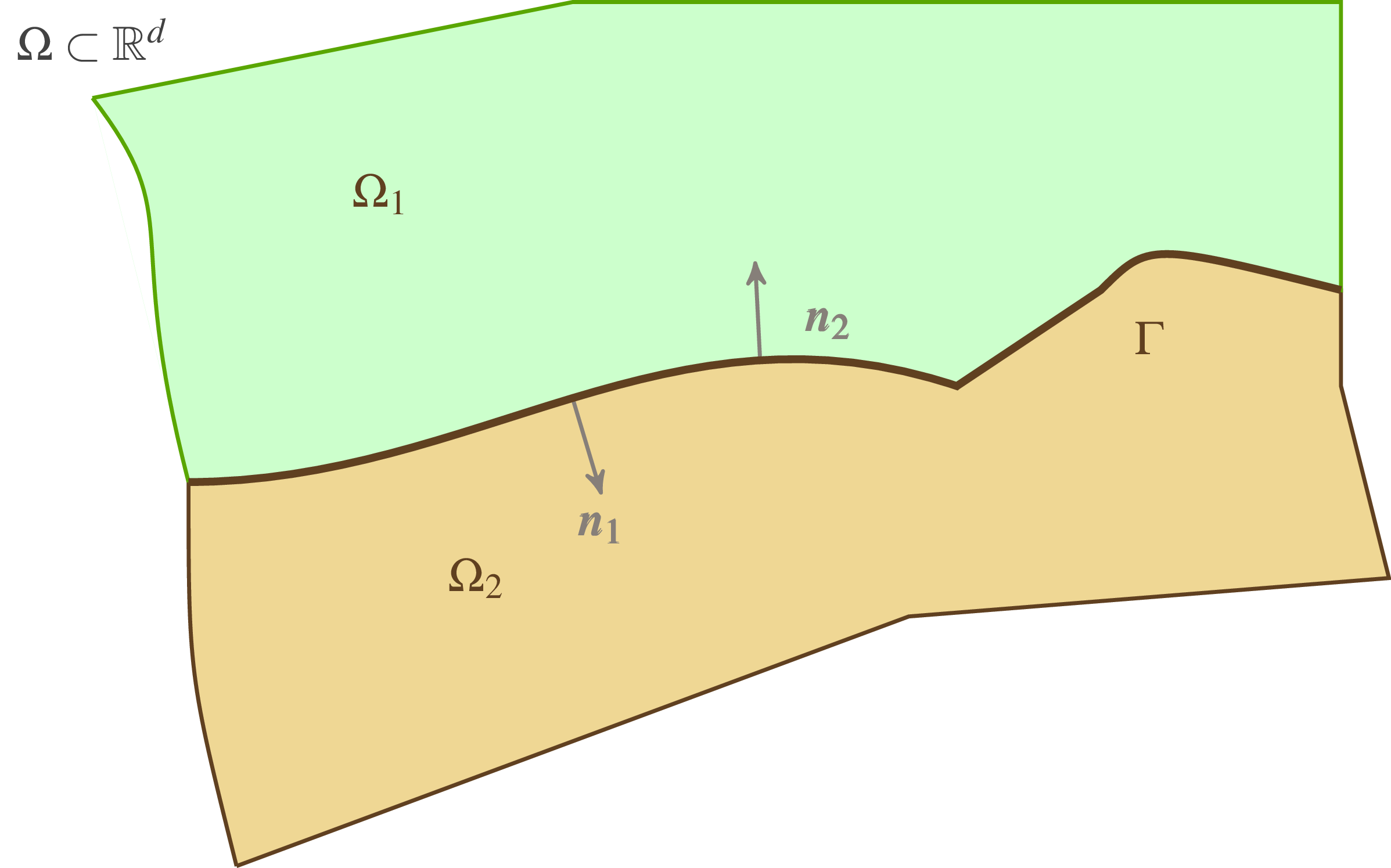
Figure 1: Illustration of the domain $\Omega=\Omega_{1}\cup\,\Omega_{2}$ $\subset\mathbb{R}^{d}$ with fixed interface $\Gamma$. Also shown are the normal vectors along the interface.

2 Problem formulation and iterative scheme

2.1 Problem formulation

Recall that $T>0$ and $\Omega\subset\mathbb{R}^{d}$ is a bounded Lipschitz domain partitioned in two subdomains $\Omega_{1,2}$, separated by the Lipschitz-continuous interface $\Gamma$. The boundary of $\Omega$ is denoted by $\partial\Omega$ and the portions of $\partial\Omega$ that are also boundaries of $\Omega_{l}$ are denoted by $\partial\Omega_{l}$ (see also Fig. 1). To ease the presentation, the two subdomains are assumed to be homogeneous and isotropic, i.e. we can have two different relative permeabilities $k_{r}=k_{r,l}$ on each $\Omega_{l}$, the intrinsic permeabilities $\bm{K}=K_{l}$ are scalar and the two porosities $\Phi_{l}$ ($l=1,2$) are constant. The product $\frac{K_{l}\,k_{r,l}}{\Phi_{l}\mu_{l}}$ in (1) is abbreviated by $k_{l}$ henceforth. We solve equation (1) in $\Omega$ together with initial and homogeneous Dirichlet boundary conditions. We refer to [47, 52] for more general conditions, including outflow-type ones.

On the two subdomains, the problem transforms into two subproblems, coupled through two conditions at the interface $\Gamma$: the continuity of the normal fluxes and the continuity of the pressures. With the fluxes $\bm{F_{l}}:=-k_{l}\bigl{(}S_{l}(p_{l})\bigr{)}\bm{\bm{\nabla}\bigl{(}}p_{l}+z\bigr{)}$, (1) becomes

$$\partial_{t}S_{l}(p_{l})+\bm{\nabla}\cdot\bm{F_{l}} =0 \mbox{in }\Omega_{l}\times(0,T],$$ (2)

$$\bm{F_{1}}\cdot\bm{n_{1}} =-\bm{F_{2}}\cdot\bm{n_{2}} \mbox{on }\Gamma\times[0,T],$$ (3)

$$p_{1} =p_{2} \mbox{on }\Gamma\times(0,T],$$ (4)

$$p_{l} =0 \mbox{on }\partial\Omega_{l}\times(0,T].$$ (5)

This is closed by the initial conditions $p_{l}(\cdot,0):=p_{l,0}$ in $\Omega_{l}$, where $p_{l}$ is the water pressure on $\Omega_{l}$, $l=1,2$, and $k_{l}$ are (given) scaled relative permeability functions, that are assumed to be smooth enough. In the above, $\bm{n_{l}}$ stands for the outer unit normal vector at $\partial\Omega_{l}$.

Semi-discrete formulation (discretisation in time)

For the time discretisation we let $N\in\mathbb{N}$ be a given and $\tau:=\tfrac{T}{N}$ be the corresponding time step. Then $p_{l}^{n}$ is the approximation of the pressure $p_{l}$ at time $t^{n}=n\tau$. The Euler implicit discretisation of (2) – (5) reads

$$S_{l}\bigl{(}p_{l}^{n}\bigr{)}-S_{l}\bigl{(}p_{l}^{n-1}\bigr{)}+\tau\bm{\nabla}\cdot\bm{F^{n}_{l}} =0 \mbox{in }\Omega_{l},$$ (6)

$$\bm{F^{n}_{1}}\cdot\bm{n_{1}} =-\bm{F^{n}_{2}}\cdot\bm{n_{2}} \mbox{on }\Gamma,$$ (7)

$$p_{1}^{n} =p_{2}^{n} \mbox{on }\Gamma,$$ (8)

$$p_{l}^{n} =0 \mbox{on }\partial\Omega^{l},$$ (9)

where $\bm{F^{n}_{l}}:=k_{l}\bigl{(}S_{l}(p_{l}^{n})\bigr{)}\bm{\nabla}\bigl{(}p_{l}^{n}+z\bigr{)}$ is the flux at time step $t^{n}$. Observe that (7) and (8) are the coupling conditions at the interface $\Gamma$.

2.2 The LDD iterative scheme

If $\bigl{(}p_{1}^{n-1},p_{2}^{n-1}\bigr{)}$ is known, $\bigl{(}p_{1}^{n},p_{2}^{n}\bigr{)}$ can be obtained by solving the nonlinear system (6)–(9). To this end, we define an iterative scheme that uses Robin type conditions at $\Gamma$ to decouple the subproblems in $\Omega_{l}$, and linearises the terms due to the saturation-pressure dependency by adding stabilisation terms that cancel each other in the limit (see e.g. [33, 31]). Specifically, assuming that for some $i\in\mathbb{N}$ the approximations $p_{l}^{n,i-1}$ and $g_{l}^{i-1}$ are known, we seek $\bigl{(}p_{1}^{n,i},p_{2}^{n,i}\bigr{)}$ solving the problems

$$L_{l}p_{l}^{n,i}-L_{l}p_{l}^{n,i-1}+\tau\bm{\nabla}\cdot\bm{F_{l}^{n,i}} =-S_{l}\bigl{(}p_{l}^{n,i-1}\bigr{)}+S_{l}\bigl{(}p_{l}^{n-1}\bigr{)} \mbox{ in }\Omega_{l},$$ (10)

$$\bm{F_{l}^{n,i}}\cdot\bm{n_{l}} =g^{i}_{l}+\lambda p_{l}^{n,i} \mbox{ on }\Gamma\times[0,T],$$ (11)

$$g_{l}^{i}: =-2\lambda p_{3-l}^{n,i-1}-g_{3-l}^{i-1}.$$ (12)

Following the previously introduced notation, $\bm{F_{l}^{n,i}}:=-k_{l}\bigl{(}S_{l}(p_{l}^{n,i-1})\bigr{)}\bm{\nabla}\bigl{(}p_{l}^{n,i}+z\bigr{)}$ denotes the linearised flux at iteration $i$. By $\lambda\in(0,\infty)$, we denote a (free to be chosen) parameter used to weight the influence of the pressure on the interface conditions at $\Gamma$. The parameters $L_{l}>0$ must adhere to some mild constraints in order for the scheme to converge, which will be discussed later, but other than that, are arbitrary. The iteration starts with

$$p_{l}^{n,0}:=p_{l}^{n-1},\qquad\text{ and }\qquad g_{l}^{0}:=\bm{F^{n-1}_{l}}\cdot\bm{n_{l}}-\lambda p_{l}^{n-1},$$

and clearly, the difference $L_{l}p_{l}^{n,i}-L_{l}p_{l}^{n,i-1}$ is vanishing in case of convergence.

Remark 1.

The usage of the terms $g_{l}^{i}$ and of the parameter $\lambda$ is motivated by the following. With the notation $f_{l}^{n}:=\bm{F^{n}_{l}}\cdot\bm{n_{l}}$, the transmission conditions (7)-(8) become $f_{1}^{n}=-f_{2}^{n}$ and $p_{1}^{n}=p_{2}^{n}$. For any $\lambda\neq 0$, these are equivalent to

$$f_{1}^{n} =(-f_{2}^{n}-\lambda p_{2}^{n})+\lambda p_{1}^{n},$$ (13)

$$f_{2}^{n} =(-f_{1}^{n}-\lambda p_{1}^{n})+\lambda p_{2}^{n}.$$

Denoting the terms between brackets by $g_{l}$, one obtains

$$\begin{aligned} f_{1}^{n}&=g_{1}+\lambda p_{1}^{n},\\ f_{2}^{n}&=g_{2}+\lambda p_{2}^{n},\end{aligned}\quad\text{ and }\quad\begin{aligned} g_{1}&=-2\lambda p_{2}^{n}-g_{2},\\ g_{2}&=-2\lambda p_{1}^{n}-g_{1}.\end{aligned}$$ (14)

The conditions in (11)-(12) are the linearised counterparts of (14).

Remark 2 (different decoupling formulations).

The decoupled conditions in (7)-(8) can be formulated as convex combinations of the terms $g$ and $p$, namely

$$\bm{F_{l}^{n,i}}\cdot\bm{n_{l}} =(1-\lambda)g^{i}_{l}+\lambda p_{l}^{n,i}$$ (11’)

$$(1-\lambda)g_{l}^{i}: =-2\lambda p_{3-l}^{n,i-1}-(1-\lambda)g_{3-l}^{i-1}.$$ (12’)

The convergence analysis below can be carried out for this formulation without any difficulty. However, the DD scheme using this convex formulation showed a slower convergence in the numerical experiments than when (11)-(12) was used. Moreover, it is easier to find close to optimal parameters for the latter. Such aspects are discussed in Section 4. In view of this, in what follows we restrict the analysis to the initial formulation.

Before formulating the main result we specify the notation that will be used below.

Notation 1.

$L^{2}(\Omega)$ is the space of Lebesgue measurable, square integrable functions over $\Omega$. $H^{1}(\Omega)$ contains functions in $L^{2}(\Omega)$ having also weak derivatives in $L^{2}(\Omega)$. $H_{0}^{1}(\Omega)=\overline{C_{0}^{\infty}(\Omega)}{}^{H^{1}}$, where the completion is with respect to the standard $H^{1}$ norm and $C_{0}^{\infty}(\Omega)$ is the space of smooth functions with compact support in $\Omega$. The definition for $H^{1}(\Omega_{l})$ ($l=1,2$) is similar. With $\Gamma$ being a $(d-1)$ dimensional manifold in $\bar{\Omega}$, $H^{\frac{1}{2}}(\Gamma)$ contains the traces of $H^{1}$ functions on $\Gamma$ (see e.g. [53, 54, 34]. Given $u\in H^{1}(\Omega)$, by its trace on $\Gamma$ is denoted by ${u}{}{|_{\Gamma}}$.

Furthermore, the following spaces will be used

$$\mathcal{V}_{l} :=\left\{u\in H^{1}(\Omega_{l})\,\bigl{|}\bigr{.}\,{u}{}{|_{\partial\Omega^{l}}}\equiv 0\right\},$$ (15)

$$\mathcal{V} :=\left\{(u_{1},u_{2})\in\mathcal{V}_{1}\times\mathcal{V}_{2}\,\bigl{|}\bigr{.}\,{u_{1}}_{|_{\Gamma}}\equiv{u_{2}}_{|_{\Gamma}}\right\},$$ (16)

$$H^{1/2}_{00}(\Gamma) \hskip 3.1pt=\bigl{\{}\nu\in H^{1/2}(\Gamma)\,\bigl{|}\bigr{.}\,\nu={w}{|_{\Gamma}}\mbox{ for a }w\in H_{0}^{1}(\Omega)\bigr{\}}.$$ (17)

Note, that $\mathcal{V}=H^{1}_{0}(\Omega)$. $H^{1/2}_{00}(\Gamma)^{\prime}$ denotes the dual space of $H^{1/2}_{00}(\Gamma)$. $\langle\cdot,\cdot\rangle_{X}$ will denote the $L^{2}(X)$ scalar product, with $X$ being one of the sets $\Omega$, $\Omega_{l}$ ($l=1,2$) or $\Gamma$. Whenever self understood, the notation of the domain of integration $X$ will be dropped. Furthermore, $\bigl{\langle}\cdot,\cdot\bigr{\rangle}_{\Gamma}$ stands also for the duality pairing between $H^{1/2}_{00}(\Gamma)^{\prime}$ and $H^{1/2}_{00}(\Gamma)$.

In what follows we make the following

Assumptions 1.

With $l=1,2$, we assume that

1. $k_{l}:\mathbb{R}\rightarrow[0,1]$ are strictly monotonically increasing and Lipschitz continuous functions with Lipschitz constants $L_{k_{l}}>0$,

2. there exists $m\in\mathbb{R}$ such that $0<m\leq k_{1}(S)$, $k_{2}(S)$ for all $S\in\mathbb{R}$,

3. $S_{l}:\mathbb{R}\rightarrow\mathbb{R}$ are monotonically increasing and Lipschitz continuous functions with Lipschitz constants $L_{S_{l}}>0$.

For later use we define $L_{k}:=\max\{$ $L_{k_{1}},L_{k_{2}}\}$ and $L_{S}:=\max\{L_{S_{1}},L_{S_{2}}\}$.

In a simplified formulation, the main result in this paper is

Theorem 1.

Assume there exists a solution pair $(p_{1}^{n},p_{2}^{n})$ to (6)–(9) that additionally fulfils $\sup_{l}\lVert\bm{\nabla}\bigl{(}p_{l}^{n}+z\bigr{)}\rVert_{L^{\infty}}\leq M<\infty$. Let $L_{l}$ obey $L_{S_{l}}<2L_{l}$ for $l=1,2$ and assume that the time step $\tau>0$ is chosen small enough, so that for both $l$ one has

$$\tau<\frac{2m}{L_{k_{l}}^{2}M^{2}}\left(\frac{1}{L_{S_{l}}}-\frac{1}{2L_{l}}\right).$$ (18)

Then the sequence of solution pairs $\bigl{\{}(p_{1}^{n,i},p_{2}^{n,i})\bigr{\}}_{i\geq 1}$ of (10)–(11) converges to $(p_{1}^{n},p_{2}^{n})$.

Remark 3.

The precise form of Theorem 1 will be formulated in Section 3, after having defined a weak solution. The theorem above is given for the ease of presentation.

3 Analysis of the scheme.

This section gives the convergence proof for the proposed scheme. The starting point is the Euler implicit discretisation in Section 2. Assuming $\bigl{(}p_{1}^{n-1},p_{2}^{n-1}\bigr{)}\in\mathcal{V}$ to be known, a weak formulation of (6)–(9) is given by

Problem 1 (Semi-discrete weak formulation).

Find $(p_{1}^{n}$, $p_{2}^{n})\in\mathcal{V}$ such that $\bm{F^{n}_{l}}\cdot\bm{n_{l}}\in H^{1/2}_{00}(\Gamma)^{\prime}$ for $l=1,2$ and

$$\bigl{\langle}S_{l}(p_{l}^{n}),\varphi_{l}\bigr{\rangle}-\tau\bigl{\langle}\bm{F^{n}_{l}},\bm{\nabla}\varphi_{l}\bigr{\rangle}+\tau\bigl{\langle}\bm{F^{n}_{3-l}} \cdot\bm{n_{l}},{\varphi_{l}}{|_{\Gamma}}\bigr{\rangle}_{\Gamma}=\bigl{\langle}S_{1}(p_{1}^{n-1}),\varphi_{1}\bigr{\rangle},$$ (19)

for all $(\varphi_{1},\varphi_{2})\in\mathcal{V}$.

Remark 4.

If $(p_{1}^{n},p_{2}^{n})\in\mathcal{V}$ is a solution of Problem 1, we have ${p_{1}^{n}}{|_{\Gamma}}={p_{2}^{n}}{|_{\Gamma}}$ by definition of $\mathcal{V}$. Testing in (19) by an arbitrary $\varphi_{l}\in C_{0}^{\infty}(\Omega_{l})$ shows that the distribution $\operatorname{\bm{\nabla}\cdot}\bm{F^{n}_{l}}$ is regular and in $L^{2}$, yielding $\bm{F^{n}_{l}}\in H(\mbox{div},\Omega_{l})$ and

$$S_{l}(p_{l}^{n})-S_{l}(p_{l}^{n-1}) =-\tau\operatorname{\bm{\nabla}\cdot}\bm{F^{n}_{l}}\qquad\mbox{a. e. in }\Omega_{l}$$ (20)

by the variational lemma. By Lemma III. 1.1 in [53], $\bm{F^{n}_{l}}\cdot\bm{n_{l}}\in H^{-1/2}(\partial\Omega_{l})$ and integrating by parts in (19) yields

$$0 =-\bigl{\langle}\bm{F^{n}_{l}}\cdot\bm{n_{l}},{\varphi_{l}}{|_{\Gamma}}\bigr{\rangle}_{\Gamma}+\bigl{\langle}\bm{F^{n}_{3-l}}\cdot\bm{n_{l}},{\varphi_{l}}{|_{\Gamma}}\bigr{\rangle}_{\Gamma}$$ (21)

for all $(\varphi_{1},\varphi_{2})\in\mathcal{V}$. Therefore

$$\bm{F^{n}_{l}}\cdot\bm{n_{l}}=\bm{F^{n}_{3-l}}\cdot\bm{n_{l}}$$ (22)

in $H^{1/2}_{00}(\Gamma)^{\prime}$ since the trace is a surjective operator.

Note additionally that Problem 1 is equivalent to the semi-discrete Richards equation on the whole domain, namely to find $(p_{1}^{n},p_{2}^{n})$ $\in\mathcal{V}$ such that

$$\bigl{\langle}S_{1}(p_{1}^{n}) ,\varphi_{1}\bigr{\rangle}-\tau\bigl{\langle}\bm{F^{n}_{1}},\bm{\nabla}\varphi_{1}\bigr{\rangle}+\bigl{\langle}S_{2}(p_{2}^{n}),\varphi_{2}\bigr{\rangle}-\tau\bigl{\langle}\bm{F^{n}_{2}},\bm{\nabla}\varphi_{2}\bigr{\rangle}=\bigl{\langle}S_{1}(p_{1}^{n-1}),\varphi_{1}\bigr{\rangle}+\bigl{\langle}S_{2}(p_{2}^{n-1}),\varphi_{2}\bigr{\rangle},$$ (23)

for all $(\varphi_{1},\varphi_{2})\in\mathcal{V}$.

Remark 5.

By applying a Kirchhoff transform in each subdomain $\Omega_{l}$, Problem 1 can be reformulated as a nonlinear transmission problem. The existence and uniqueness of a solution for such problems has been studied in [55, 56] for the case when $\Omega_{1}$ is surrounded by $\Omega_{2}$, and the common boundary is smooth, however.

Now we can give the weak form of the iterative scheme. Let $n\in\mathbb{N}$ and assume that the pair $\bigl{(}p_{1}^{n-1}$, $p_{2}^{n-1}\bigr{)}\in\mathcal{V}$ is given. Furthermore, let $\lambda>0$ and $L_{l}>0$ ($l=1,2$) be fixed parameters and

$$p_{l}^{n,0}:=p_{l}^{n-1},\quad\text{ as well as }\quad g_{l}^{0}:=\bm{F^{n-1}_{l}}\cdot\bm{n_{l}}-\lambda{p_{l}^{n-1}}{}{|_{\Gamma}}.$$

The iterative scheme is defined through

Problem 2 ($L$-scheme, weak form).

Let $i\in\mathbb{N}$ and assume that the approximations $\bigl{\{}p_{l}^{n,k}\bigr{\}}_{k=0}^{i-1}$ and $\bigl{\{}g_{l}^{k}\bigr{\}}_{k=0}^{i-1}$ are known for $l=1,2$. Find $\bigl{(}p_{1}^{n,i},p_{2}^{n,i}\bigr{)}\in\mathcal{V}$ such that

$$L_{l}\bigl{\langle}p_{l}^{n,i},\varphi_{l}\bigr{\rangle}-\tau\bigl{\langle}\bm{F_{l}^{n,i}},\bm{\nabla}\varphi_{l}\bigr{\rangle}+\tau\bigl{\langle}\lambda p_{l}^{n,i}+g_{l}^{i},\varphi_{l}\bigr{\rangle}_{\Gamma} =L_{l}\bigl{\langle}p_{l}^{n,i-1},\varphi_{l}\bigr{\rangle}-\bigl{\langle}S_{l}(p_{l}^{n,i-1})-S_{l}\bigl{(}p_{l}^{n-1}\bigr{)},\varphi_{l}\bigr{\rangle}$$ (24)

$$\bigl{\langle}g_{l}^{i},\varphi_{l}\bigr{\rangle}_{\Gamma}\,\, :=\bigl{\langle}-2\lambda{p_{3-l}^{n,i-1}}-g_{3-l}^{i-1},\varphi_{l}\bigr{\rangle}_{\Gamma}$$ (25)

holds for all $(\varphi_{1},\varphi_{2})\in\mathcal{V}$.

3.1 Intuitive justification of the $L$-scheme

We start the analysis by taking a closer look at the formal limit of the $L$-scheme iterations in weak form and show that this is actually a reformulation of Problem 1.

Lemma 2 (Limit of the $L$-scheme).

Let $n\in\mathbb{N}$ be fixed and assume that the functions $p_{l}^{n}\in\mathcal{V}_{l}$ and $g_{l}\in H^{1/2}_{00}(\Gamma)^{\prime}$ ($l=1,2$) exist such that

$$\bigl{\langle}S_{l}(p_{l}^{n}),\varphi_{l}\bigr{\rangle}-\bigl{\langle}S_{l}\bigl{(}p_{l}^{n-1}\bigr{)} ,\varphi_{l}\bigr{\rangle}-\tau\bigl{\langle}\bm{F^{n}_{l}},\bm{\nabla}\varphi_{l}\bigr{\rangle}+\tau\bigl{\langle}\lambda p^{n}_{l},+g_{l},\varphi_{l}\bigr{\rangle}_{\Gamma}=0,$$ (26)

$$\bigl{\langle}g_{l},\varphi_{l}\bigr{\rangle}_{\Gamma}=\bigl{\langle} -2\lambda p_{3-l}^{n}-g_{3-l},\varphi_{l}\bigr{\rangle}_{\Gamma},$$ (27)

hold for all $(\varphi_{1},\varphi_{2})\in\mathcal{V}$. Then the interface conditions

$${p_{1}^{n}}{|_{\Gamma}} ={p_{2}^{n}}{|_{\Gamma}} \mbox{ in }H^{1/2}_{00}(\Gamma),$$ (28)

$$\bm{F^{n}_{1}}\cdot\bm{n_{1}} =\bm{F^{n}_{2}}\cdot\bm{n_{1}} \mbox{ in }H^{1/2}_{00}(\Gamma)^{\prime}$$ (29)

are satisfied and $(p_{1}^{n},p_{2}^{n})$ solves Problem 1. Moreover,

$$g_{l}=-\lambda{p_{l}^{n}}{|_{\Gamma}}+\bm{F^{n}_{l}}\cdot\bm{n_{l}}$$ (30)

in $H^{1/2}_{00}(\Gamma)^{\prime}$. Conversely, if $(p_{1}^{n},p_{2}^{n})\in\mathcal{V}$ is a solution of Problem 1 and $g_{l}:=-\lambda{p_{l}^{n}}{|_{\Gamma}}+\bm{F^{n}_{l}}\cdot\bm{n_{l}}$, then $p_{l}^{n}$ and $g_{l}$ solve the system (26), (27).

Remark 6.

Lemma 2 states that solving Problem 1 is equivalent to finding a solution to (26), (27). This reformulation will be used to show, that the L-scheme converges to a solution of Problem 1

Proof.

Writing out (27) for $l=1,2$ and subtracting the resulting equations yields ${p_{1}^{n}}{|_{\Gamma}}={p_{2}^{n}}{|_{\Gamma}}$ in the sense of traces. On the other hand, adding up these equations leads to $(g_{1}+g_{2})=-\lambda({p_{1}^{n}}{|_{\Gamma}}+{p_{2}^{n}}{|_{\Gamma}})$. Inserting this into the sum of the equations (26) leads to (23), and by equivalence to the semi-discrete formulation (19). Moreover, by (20) one has $S_{l}(p_{l}^{n})-S_{l}(p_{l}^{n-1})=-\tau\operatorname{\bm{\nabla}\cdot}\bm{F^{n}_{l}}$ a.e. and therefore integrating by parts in (26) gives $g_{l}=-\lambda{p_{l}^{n}}{|_{\Gamma}}+\bm{F^{n}_{l}}\cdot\bm{n_{l}}$ in $H^{1/2}_{00}(\Gamma)^{\prime}$.

Conversely, if $(p_{1}^{n},p_{2}^{n})$ solves Problem 1, then ${p_{1}^{n}}{|_{\Gamma}}={p_{2}^{n}}{|_{\Gamma}}$ and

$$g_{l}=-\lambda{p_{l}^{n}}{|_{\Gamma}} +\bm{F^{n}_{l}}\cdot\bm{n_{l}}=-\lambda{p_{3-l}^{n}}{|_{\Gamma}}+\bm{F^{n}_{3-l}}\cdot\bm{n_{3-l}}=-2\lambda{p_{3-l}^{n}}{|_{\Gamma}}-g_{3-l}$$ (31)

is deduced by the flux continuity (22). Finally, (26) now follows by integrating (20) by parts and using the definition of $g_{l}$. ∎

3.2 Convergence of the scheme

The convergence of the $L$-scheme involves two steps: first, we prove the existence and uniqueness of a solution to Problem 2 defining the linear iterations, and then we prove the convergence of the sequence of such solutions to the expected limit.

Lemma 3.

Problem 2 has a unique solution.

Proof.

This is a direct consequence of the Lax-Milgram lemma. ∎

We now prove the convergence result, which was announced in Theorem 1. We assume that the solution $\bigl{(}p_{1}^{n-1},p_{2}^{n-1}\bigr{)}$ of Problem 1 at time step $(n-1)$ is known and let $p_{l}^{n,0}\in\mathcal{V}_{l}$ be arbitrary starting pressures (however, a natural choice is $p_{l}^{n,0}:=p_{l}^{n-1}$).

Lemma 3 enables us to construct a sequence $\bigl{\{}p_{l}^{n,i}\bigr{\}}_{i\in\mathbb{N}_{0}}\in\mathcal{V}_{l}^{\mathbb{N}}$ of solutions to Problem 2 and prove its convergence to the solution $\bigl{(}p_{1}^{n},p_{2}^{n}\bigr{)}$ of Problem 1 at the subsequent time step.

Theorem 4 (Convergence of the DD scheme).

Assume there exists a solution $(p_{1}^{n},p_{2}^{n})\in\mathcal{V}$ to Problem 1 s.t. $\sup_{l}\lVert\bm{\nabla}\bigl{(}p_{l}^{n}+z\bigr{)}\rVert_{L^{\infty}}\leq M<\infty$ and let $g_{l}$ be as in (30). Let Assumptions 1 hold, $\lambda>0$ and $L_{l}\in\mathbb{R}$ be given with $L_{S_{l}}/2<L_{l}$ for $l=1,2$. For arbitrary starting pressures $p_{l}^{n,0}:=v_{l,0}\in\mathcal{V}_{l}$ $(l=1,2)$ let $\bigl{\{}(p_{1}^{n,i},p_{2}^{n,i})\bigr{\}}_{i\in\mathbb{N}_{0}}$ be the sequence of solutions of Problem 2 and let $\bigl{\{}g_{l}^{i}\bigr{\}}_{i\in\mathbb{N}_{0}}$ be defined by (25). Assume further that the time step $\tau$ satisfies

$$\tau<\frac{2m}{L_{k_{l}}^{2}M^{2}}\left(\frac{1}{L_{S_{l}}}-\frac{1}{2L_{l}}\right).$$ (32)

Then $p_{l}^{n,i}\rightarrow p_{l}^{n}$ in $\mathcal{V}_{l}$ and $g_{l}^{i}\rightarrow g_{l}$ in $\mathcal{V}_{l}^{\prime}$ as $i\rightarrow\infty$ for $l=1,2$.

Remark 7.

The essential boundedness of the pressure gradients can be proven under the additional assumption that the functions $S_{l}$ are strictly increasing and the domain is of class $C^{1,\alpha}$, see e.g. [57, Lemma 2.1].

Proof.

We introduce the iteration errors $e_{p,l}^{i}:=p_{l}^{n}-p_{l}^{n,i}$ as well as $e_{g,l}^{i}:=g_{l}^{n}-g_{l}^{i}$, add $L_{l}\langle p_{l}^{n},\varphi_{l}\rangle-L_{l}\langle p_{l}^{n},\varphi_{l}\rangle$ to (26) and subtract (24) to arrive at

$$L_{l} \bigl{\langle}e_{p,l}^{i},\varphi_{l}\bigr{\rangle}+\tau\lambda\bigl{\langle}e_{p,l}^{i},\varphi_{l}\bigr{\rangle}_{\Gamma}+\tau\bigl{\langle}e_{g,l}^{i},\varphi_{l}\bigr{\rangle}_{\Gamma}+\tau\Bigl{[}\Bigl{\langle}-\bm{F^{n}_{l}}{-\,k_{l}\bigl{(}S_{l}(p_{l}^{n,i-1})\bigr{)}\bm{\nabla}\bigl{(}p_{l}^{n}+z\bigr{)}}$$

$${\,+\,k_{l}\bigl{(}S_{l}(p_{l}^{n,i-1})\bigr{)}\bm{\nabla}\bigl{(}p_{l}^{n}+z\bigr{)}}+\bm{F_{l}^{n,i}},\bm{\nabla}\varphi_{l}\Bigr{\rangle}\Bigr{]}=L_{l}\bigl{\langle}e_{p,l}^{i-1},\varphi_{l}\bigr{\rangle}-\bigl{\langle}S_{l}(p_{l}^{n})-S_{l}(p_{l}^{n,i-1}),\varphi_{l}\bigr{\rangle}.$$ (33)

Inserting $\varphi_{l}:=e_{p,l}^{i}$ in (33) and noting that

$$L_{l}\Bigl{\langle}e_{p,l}^{i}-e_{p,l}^{i-1},e_{p,l}^{i}\Bigr{\rangle} =\frac{L_{l}}{2}\Bigl{[}\bigl{\|}e_{p,l}^{i}\bigr{\|}^{2}-\bigl{\|}e_{p,l}^{i-1}\bigr{\|}^{2}+\bigl{\|}e_{p,l}^{i}-e_{p,l}^{i-1}\bigr{\|}^{2}\Bigr{]},$$

yields

$$\frac{L_{l}}{2} \Bigl{[}\bigl{\|}e_{p,l}^{i}\bigr{\|}^{2}-\bigl{\|}e_{p,l}^{i-1}\bigr{\|}^{2}+\bigl{\|}e_{p,l}^{i}-e_{p,l}^{i-1}\bigr{\|}^{2}\Bigr{]}\underbrace{{+\bigl{\langle}S_{l}(p_{l}^{n})-S_{l}(p_{l}^{n,i-1}),e_{p,l}^{i-1}\bigr{\rangle}}}_{=:I_{1}}+\tau\lambda\bigl{\langle}e_{p,l}^{i},e_{p,l}^{i}\bigr{\rangle}_{\Gamma}$$

$$=\underbrace{\bigl{\langle}S_{l}(p_{l}^{n})-S_{l}(p_{l}^{n,i-1}),{e_{p,l}^{i-1}}-e_{p,l}^{i}\bigr{\rangle}}_{=:I_{2}}-\tau\bigl{\langle}e_{g,l}^{i},e_{p,l}^{i}\bigr{\rangle}_{\Gamma}$$

$$-\underbrace{\tau\Bigl{\langle}\Bigl{(}k_{l}\bigl{(}S_{l}(p_{l}^{n})\bigr{)}-k_{l}\bigl{(}S_{l}(p_{l}^{n,i-1})\bigr{)}\!\Bigr{)}\bm{\nabla}\bigl{(}p_{l}^{n}+z\bigr{)},\bm{\nabla}e_{p,l}^{i}\Bigr{\rangle}}_{=:I_{3}}-\underbrace{\tau\Bigl{\langle}k_{l}\bigl{(}S_{l}(p_{l}^{n,i-1})\bigr{)}\bm{\nabla}e_{p,l}^{i},\bm{\nabla}e_{p,l}^{i}\Bigr{\rangle}.}_{=:I_{4}}$$ (34)

We estimate now the terms $I_{1}$–$I_{4}$ in (34) one by one. By Assumption 1c), for $I_{1}$ we have

$$\frac{1}{L_{S_{l}}}\bigl{\|}S_{l}(p_{l}^{n})-S_{l}(p_{l}^{n,i-1})\bigr{\|}^{2} \leq\bigl{\langle}S_{l}(p_{l}^{n})-S_{l}(p_{l}^{n,i-1}),e_{p,l}^{i-1}\bigr{\rangle}.$$ (35)

$I_{2}$ is estimated by

$$\bigl{|}I_{2}\bigr{|} =\left|\Bigl{\langle}S_{l}(p_{l}^{n})-S_{l}(p_{l}^{n,i-1}),e_{p,l}^{i-1}-e_{p,l}^{i}\Bigr{\rangle}\right|\leq\frac{L_{l}}{2}\bigl{\|}e_{p,l}^{i-1}-e_{p,l}^{i}\bigr{\|}^{2}+\frac{1}{2L_{l}}\bigl{\|}S_{l}(p_{l}^{n})-S_{l}(p_{l}^{n,i-1})\bigr{\|}^{2}.$$ (36)

For an $\epsilon_{l}>0$ to be chosen below we use Young’s inequality to deal with $I_{3}$, which can be estimated by

$$\bigl{|}I_{3}\bigr{|} =\Bigl{|}\tau\Bigl{\langle}\Bigl{(}k_{l}\bigl{(}S_{l}(p_{l}^{n})\bigr{)}-k_{l}\bigl{(}S_{l}(p_{l}^{n,i-1})\bigr{)}\!\Bigr{)}\bm{\bm{\nabla}}\bigl{(}p_{l}^{n}+z\bigr{)},\bm{\nabla}e_{p,l}^{i}\Bigr{\rangle}\Bigr{|}$$

$$\leq\tau\bigl{\|}\bigl{(}k_{l}\bigl{(}S_{l}(p_{l}^{n})\bigr{)}-k_{l}\bigl{(}S_{l}(p_{l}^{n,i-1})\bigr{)}\bigr{)}\bm{\nabla}\bigl{(}p_{l}^{n}+z\bigr{)}\bigr{\|}\bigl{\|}\bm{\nabla}e_{p,l}^{i}\bigr{\|}$$

$$\leq\tau L_{k_{l}}M\bigl{\|}S_{l}(p_{l}^{n})-S_{l}(p_{l}^{n,i-1})\bigr{\|}\bigl{\|}\bm{\nabla}e_{p,l}^{i}\bigr{\|}$$

$$\leq\tau L_{k_{l}}M\epsilon_{l}\bigl{\|}S_{l}(p_{l}^{n})-S_{l}(p_{l}^{n,i-1})\bigr{\|}^{2}+\tau\frac{L_{k_{l}}M}{4\epsilon_{l}}\bigl{\|}\bm{\nabla}e_{p,l}^{i}\bigr{\|}^{2},$$ (37)

where we used the Lipschitz continuity of $k_{l}$ and the assumption $\sup_{l}\bigl{\|}\bm{\nabla}\bigl{(}p_{l}^{n}+z\bigr{)}\bigr{\|}_{L^{\infty}}<M$. Finally, by Assumption 1b) one has

$$\tau\Bigl{\langle}k_{l}\bigl{(}S_{l}(p_{l}^{n,i-1})\bigr{)}\bm{\nabla}e_{p,l}^{i},\bm{\nabla}e_{p,l}^{i}\Bigr{\rangle}\geq\tau m\bigl{\|}\bm{\nabla}e_{p,l}^{i}\bigr{\|}^{2}$$ (38)

for $I_{4}$. Using the estimates (35)–(38), (34) becomes

$$\frac{L_{l}}{2}\Bigl{[} \bigl{\|}e_{p,l}^{i}\bigr{\|}^{2}-\bigl{\|}e_{p,l}^{i-1}\bigr{\|}^{2}\Bigr{]}+\frac{1}{L_{S_{l}}}\bigl{\|}S_{l}(p_{l}^{n})-S_{l}(p_{l}^{n,i-1})\bigr{\|}^{2}+\tau\lambda\bigl{\langle}e_{p,l}^{i},e_{p,l}^{i}\bigr{\rangle}_{\Gamma}+\tau\bigl{\langle}e_{g,l}^{i},e_{p,l}^{i}\bigr{\rangle}_{\Gamma}$$

$$\leq\left(\frac{1}{2L_{l}}+\tau L_{k_{l}}M\epsilon_{l}\right)\bigl{\|}S_{l}(p_{l}^{n})-S_{l}(p_{l}^{n,i-1})\bigr{\|}^{2}+\tau\left(\frac{L_{k_{l}}M}{4\epsilon_{l}}-m\right)\bigl{\|}\bm{\nabla}e_{p,l}^{i}\bigr{\|}^{2}.$$ (34’)

In order to deal with the interface term $\tau\bigl{\langle}e_{g,l}^{i},e_{p,l}^{i}\bigr{\rangle}_{\Gamma}$ recall, that $\bigl{\langle}\cdot,\cdot\bigr{\rangle}_{\Gamma}$ denotes the dual pairing of $H^{1/2}_{00}(\Gamma)^{\prime}$ and $H^{1/2}_{00}(\Gamma)$ and the $H^{1/2}_{00}(\Gamma)$-norm simultaneously. Subtracting (25) from (27), i.e. $e_{g,l}^{i}=-2\lambda e_{p,3-l}^{i-1}-e_{g,3-l}^{i-1}$, we get

$$\bigl{\|}e_{p,l}^{i}\bigr{\|}^{2}_{\Gamma} =\frac{1}{4\lambda^{2}}\left(\bigl{\|}e_{g,3-l}^{i+1}\bigr{\|}^{2}_{\Gamma}-\bigl{\|}e_{g,l}^{i}\bigr{\|}^{2}_{\Gamma}-4\lambda\bigl{\langle}e_{p,l}^{i},e_{g,l}^{i}\bigr{\rangle}_{\Gamma}\right).$$ (39)

With $b\in\{p,g\}$ we let $e_{b}^{i}:=(e_{b,1}^{i},e_{b,2}^{i})\in\mathcal{V}_{1}\times\mathcal{V}_{2}$ and $\lVert e_{b}^{i}\rVert^{2}:=\sum_{l=1}\lVert e_{b,l}^{i}\rVert^{2}$. Similarly, on $\Gamma$ we let $\bigl{\langle}e_{b}^{i},e_{b}^{i}\bigr{\rangle}_{\Gamma}:=\sum_{l=1}^{2}\bigl{\langle}e_{b,l}^{i},e_{b,l}^{i}\bigr{\rangle}_{\Gamma}$ and correspondingly $\lVert e_{b}^{i}\rVert_{\Gamma}^{2}=\sum_{l=1}^{2}\lVert e_{b,l}^{i}\rVert_{\Gamma}^{2}$. Summing in (39) over $l=1,2$ gets

$$\lVert e_{p}^{i}\rVert^{2}_{\Gamma} =\frac{1}{4\lambda^{2}}\Bigl{(}\lVert e_{g}^{i+1}\rVert_{\Gamma}^{2}-\lVert e_{g}^{i}\rVert^{2}_{\Gamma}-4\lambda\bigl{\langle}e_{p}^{i},e_{g}^{i}\bigr{\rangle}_{\Gamma}\Bigr{)}.$$ (40)

Doing the same for (34’) and inserting (40), leaves us with

$$\frac{L_{l}}{2} \Bigl{[}\bigl{\|}e_{p}^{i}\bigr{\|}^{2}-\bigl{\|}e_{p}^{i-1}\bigr{\|}^{2}\Bigr{]}+\sum_{l=1}^{2}\frac{1}{L_{S_{l}}}\bigl{\|}S_{l}(p_{l}^{n})-S_{l}(p_{l}^{n,i-1})\bigr{\|}^{2}$$

$$+\frac{\tau}{4\lambda}\left(\lVert e_{g}^{i+1}\rVert_{\Gamma}^{2}-\lVert e_{g}^{i}\rVert^{2}_{\Gamma}\right)+\tau\sum_{l=1}^{2}\biggl{(}m-\frac{L_{k_{l}}M}{4\epsilon_{l}}\biggr{)}\bigl{\|}\bm{\nabla}e_{p,l}^{i}\bigr{\|}^{2}$$

$$\leq\sum_{l=1}^{2}\left(\frac{1}{2L_{l}}+\tau L_{k_{l}}M\epsilon_{l}\right)\bigl{\|}S_{l}(p_{l}^{n})-S_{l}(p_{l}^{n,i-1})\bigr{\|}^{2}.$$ (41)

Now, summing for the iteration index $i=1,\dots,r$ and noticing telescopic sums one gets

$$\sum_{i=1}^{r} \sum_{l=1}^{2}\Bigl{(}\frac{1}{L_{S_{l}}}-\frac{1}{2L_{l}}-\tau L_{k_{l}}M\epsilon_{l}\Bigr{)}\bigl{\|}S_{l}(p_{l}^{n})-S_{l}(p_{l}^{n,i-1})\bigr{\|}^{2}$$

$$+\tau\sum_{i=1}^{r}\sum_{l=1}^{2}\left(m-\frac{L_{k_{l}}M}{4\epsilon_{l}}\right)\bigl{\|}\bm{\nabla}e_{p,l}^{i}\bigr{\|}^{2}$$

$$\leq\frac{L_{l}}{2}\Bigl{[}\bigl{\|}e_{p}^{0}\bigr{\|}^{2}-\bigl{\|}e_{p}^{r}\bigr{\|}^{2}\Bigr{]}+\frac{\tau}{4\lambda}\Bigl{(}\lVert e_{g}^{1}\rVert_{\Gamma}^{2}-\lVert e_{g}^{r+1}\rVert^{2}_{\Gamma}\Bigr{)}.$$ (42)

Now we choose $\epsilon_{l}=\frac{L_{k_{l}}M}{2m}$, hence $m-\frac{L_{k_{l}}M}{4\epsilon_{l}}=\frac{m}{2}>0$ for both $l$. Recalling the restriction on $L_{l}$, $\frac{1}{L_{S_{l}}}-\frac{1}{2L_{l}}>0$, as well as that by the time step restriction $\frac{1}{L_{S_{l}}}-\frac{1}{2L_{l}}-\tau\frac{L_{k_{l}}^{2}M^{2}}{2m}>0$ for $l=1,2$, the estimates

$$\sum_{i=1}^{r}\sum_{l=1}^{2}\biggl{(}\frac{1}{L_{S_{l}}}-\frac{1}{2L_{l}} -\tau\frac{L_{k_{l}}^{2}M^{2}}{2m}\biggr{)}\bigl{\|}S_{l}(p_{l}^{n})-S_{l}(p_{l}^{n,i-1})\bigr{\|}^{2}\leq\frac{L_{l}}{2}\bigl{\|}e_{p}^{0}\bigr{\|}^{2}+\frac{\tau}{4\lambda}\lVert e_{g}^{1}\rVert_{\Gamma}^{2},$$ (43)

$$\tau\sum_{i=1}^{r}\frac{m}{2}\bigl{\|}\bm{\nabla}e_{p}^{i}\bigr{\|}^{2} \leq\frac{L_{l}}{2}\bigl{\|}e_{p}^{0}\bigr{\|}^{2}+\frac{\tau}{4\lambda}\lVert e_{g}^{1}\rVert_{\Gamma}^{2}$$ (44)

follow for for any $r\in\mathbb{N}$. Since the right hand sides are independent of $r$, we thereby conclude that the series on the left are absolutely convergent and therefore $\bigl{\|}S_{l}(p_{l}^{n})-S_{l}(p_{l}^{n,i-1})\bigr{\|}$, $\bigl{\|}\bm{\nabla}e_{p,l}^{i}\bigr{\|}$ $\longrightarrow 0$ as $i\rightarrow\infty$. Moreover, (44) implies $\bigl{\|}e_{p,l}^{i}\bigr{\|}$ $\longrightarrow 0$, $(i\rightarrow\infty)$ as well, by the Poincaré inequality.

To show that $e_{g,l}^{i}\rightarrow 0$ in $\mathcal{V}_{l}^{\prime}$ we subtract again (24) from (26) and consider test functions $\varphi_{l}\in C_{0}^{\infty}(\Omega_{l})$ to get

$$-\tau\Bigl{\langle}\bm{F^{n}_{l}}-\bm{F_{l}^{n,i}},\bm{\nabla}\varphi_{l}\Bigr{\rangle} =-L_{l}\bigl{\langle}e_{p,l}^{i},\varphi_{l}\bigr{\rangle}+L_{l}\bigl{\langle}e_{p,l}^{i-1},\varphi_{l}\bigr{\rangle}-\bigl{\langle}S_{l}(p_{l}^{n})-S_{l}(p_{l}^{n,i-1}),\varphi_{l}\bigr{\rangle}.$$ (45)

Thus, $\operatorname{\bm{\nabla}\cdot}\Bigl{(}\bm{F^{n}_{l}}-\bm{F_{l}^{n,i}}\Bigr{)}$ exists in $L^{2}$ and

$$-\tau\operatorname{\bm{\nabla}\cdot}\Bigl{(}\bm{F^{n}_{l}}-\bm{F_{l}^{n,i}}\Bigr{)}=L_{l}\Bigl{(}e_{p,l}^{i}-e_{p,l}^{i-1}\Bigr{)}+S_{l}(p_{l}^{n})-S_{l}(p_{l}^{n,i-1})$$ (46)

almost everywhere. Therefore, for any $\varphi_{l}\in\mathcal{V}_{l}$ one has

$$\Bigl{|}\Bigl{\langle}\operatorname{\bm{\nabla}\cdot}\bigl{(}\bm{F^{n}_{l}}-\bm{F_{l}^{n,i}}\bigr{)},\varphi_{l}\Bigr{\rangle}\Bigr{|} \leq\frac{L_{l}}{\tau}\bigl{\|}e_{p,l}^{i}-e_{p,l}^{i-1}\bigr{\|}\bigl{\|}\varphi_{l}\bigr{\|}+\frac{1}{\tau}\bigl{\|}S_{l}(p_{l}^{n})-S_{l}(p_{l}^{n,i-1})\bigr{\|}\bigl{\|}\varphi_{l}\bigr{\|}.$$ (47)

Abbreviating the left hand side of (47) as $\bigl{|}\Psi_{l}^{n,i}\bigl{(}\varphi_{l}\bigr{)}\bigr{|}$, (47) means

$$\sup_{\stackrel{{\scriptstyle\varphi_{l}\in\mathcal{V}_{l}}}{{\varphi_{l}\neq 0}}} \frac{\bigl{|}\Psi_{l}^{n,i}\bigl{(}\varphi_{l}\bigr{)}\bigr{|}}{\lVert\varphi_{l}\rVert_{\mathcal{V}_{l}}}\leq\frac{L_{l}}{\tau}\bigl{\|}e_{p,l}^{i}-e_{p,l}^{i-1}\bigr{\|}+\frac{1}{\tau}\bigl{\|}S_{l}(p_{l}^{n})-S_{l}(p_{l}^{n,i-1})\bigr{\|}\longrightarrow 0\quad(i\rightarrow\infty)$$ (48)

as a consequence of (44). In other words $\bigl{\|}\Psi_{l}^{n,i}\bigr{\|}_{\mathcal{V}_{l}^{\prime}}\rightarrow 0$ as $i\rightarrow\infty$. Starting again from (33) (without the added zero term), this time however inserting $\varphi_{l}\in\mathcal{V}_{l}$, integrating by parts and keeping in mind (46) one gets

$$\bigl{\langle}e_{g,l}^{i},\varphi_{l}\bigr{\rangle}_{\Gamma}=-\lambda \bigl{\langle}e_{p,l}^{i},\varphi_{l}\bigr{\rangle}_{\Gamma}+\Bigl{\langle}\bigl{[}\bm{F^{n}_{l}}-\bm{F_{l}^{n,i}}\bigr{]}\cdot\bm{n_{l}},\varphi_{l}\Bigr{\rangle}_{\Gamma}.$$ (49)

We already know that $\bigl{\|}e_{p,l}^{i}\bigr{\|}_{\mathcal{V}_{l}}\rightarrow 0$ as $i\rightarrow 0$ so by the continuity of the trace operator the first term on the right vanishes in the limit. For the last summand in (49) we use the integration by parts formula to obtain

$$\Bigl{\langle}\bigr{[}\bm{F^{n}_{l}}-\bm{F_{l}^{n,i}}\bigr{]}\cdot\bm{n_{l}},{\varphi_{l}}{|_{\Gamma}}\Bigr{\rangle}_{\Gamma} =\Psi_{l}^{n,i}(\varphi_{l})+\Bigl{\langle}\bm{F^{n}_{l}}-\bm{F_{l}^{n,i}},\bm{\nabla}\varphi_{l}\Bigr{\rangle}.$$ (50)

While the first term on the right approaches 0, the second can be estimated by

$$\Bigl{|}\Bigl{\langle}k_{l}\bigl{(}S_{l}(p_{l}^{n})\bigr{)}\bm{\nabla}\bigl{(}p_{l}^{n}+z\bigr{)} -k_{l}\bigl{(}S_{l}(p_{l}^{n,i-1})\bigr{)}\bm{\nabla}\bigl{(}p_{l}^{n,i}+z\bigr{)},\bm{\nabla}\varphi_{l}\Bigr{\rangle}\Bigr{|}$$

$$\leq L_{k_{l}}M\bigl{\|}S\bigl{(}p_{l}^{n}\bigr{)}-S\bigl{(}p_{l}^{n,i-1}\bigr{)}\bigr{\|}\bigl{\|}\varphi_{l}\bigr{\|}_{\mathcal{V}_{l}}+\bigl{\|}\bm{\nabla}p_{l}^{n,i}\bigr{\|}\bigl{\|}\varphi_{l}\bigr{\|}_{\mathcal{V}_{l}},$$ (51)

where we used the same reasoning as in (37). With this we let $i\rightarrow\infty$ in (50) to obtain

$$\sup_{\stackrel{{\scriptstyle\varphi_{l}\in\mathcal{V}_{l}}}{{\lVert\varphi_{l}\rVert_{\mathcal{V}_{l}}=1}}} \Bigl{|}\Bigl{\langle}\bigr{[}\bm{F^{n}_{l}}-\bm{F_{l}^{n,i}}\bigr{]}\cdot\bm{n_{l}},\varphi_{l}\Bigr{\rangle}_{\Gamma}\Bigr{|}\leq\bigl{\|}\Psi_{l}^{n,i}\bigr{\|}_{\mathcal{V}_{l}^{\prime}}+L_{k_{l}}M\bigl{\|}S\bigl{(}p_{l}^{n}\bigr{)}-S\bigl{(}p_{l}^{n,i-1}\bigr{)}\bigr{\|}+\bigl{\|}\bm{\nabla}p_{l}^{n,i}\bigr{\|}\longrightarrow 0.$$ (52)

Finally, using the above and letting $i\rightarrow\infty$ in (49) gives

$$\sup_{\stackrel{{\scriptstyle\varphi_{l}\in\mathcal{V}_{l}}}{{\varphi_{l}\neq 0}}} \frac{\bigl{|}\bigl{\langle}e_{g,l}^{i},\varphi_{l}\bigr{\rangle}_{\Gamma}\bigr{|}}{\lVert\varphi_{l}\rVert_{\mathcal{V}_{l}}}\longrightarrow 0.$$

This shows $e_{g,l}^{i}\rightarrow 0$ in $\mathcal{V}_{l}^{\prime}$ for both $l$ and concludes the proof. ∎

Remark 8.

Note that Theorem 4 states that if a solution to the semi-discrete coupled problem exists, then it is the limit of the iteration scheme. Since in the convergence proof we use the existence of a solution to Problem 1, the argument cannot be used to prove existence. The difficulty lies in the fact that the nonlinearities encountered in the diffusion terms are space dependent and may be discontinuous w.r.t. $x$ over the interface.

4 Numerical Experiments

This section is devoted to numerical experiments and the implementation of the proposed domain decomposition L-scheme. As our formulation and analysis did not specialise to a particular spacial discretisation, the numerical implementation of the LDD scheme can in principal be done with finite difference, finite elements as well as finite volume schemes. Since mass conservation is an essential feature of porous media flow models, we adopted a cell-centred two point flux approximation variant of a finite volume scheme to reflect this on the numerical level. The domain $\Omega$ is assumed to be rectangular and a rectangular uniform mesh was used.

Remark 9 (different decoupling formulations revisited).

We saw in Remark 2 that another decoupling formulation is possible. In fact, this can be taken a step further. Equations (11), (12) as well as (11’), (12’) can be embedded into a combined formulation. For some $0<\eta<1$ and $M>0$, consider the generalised decoupling

$$\bm{F_{l}^{n,i}}\cdot\bm{n_{l}} =M\left[(1-\eta)g^{i}_{l}+\eta p_{l}^{n,i}\right],$$ (11’’)

$$(1-\eta)g_{l}^{i} =-2\eta p_{3-l}^{n,i-1}-(1-\eta)g_{3-l}^{i-1}.$$ (12’’)

Observe that the $\lambda$-formulation (11), (12), as well as the convex-combination formulation (11’), (12’), are special cases of this general formulation: In particular, $M=(1-\eta)^{-1}$ and $\lambda=\eta(1-\eta)^{-1}$ recovers the $\lambda$-formulation, $M=1$ and $\eta=\lambda$ yields the convex-combination formulation. Although (11’’) and (12’’) might give even greater parametric control over the numerics, in this paper we adhere to the $\lambda$-formulation because of its simplicity. Fig. 10 and Fig. 12 show the influence of $\lambda$ and $\eta$ in both formulations.

We start by considering an analytically solvable example. The LDD scheme is tested against other frequently used schemes that do not use a domain decomposition. All of them are defined on the entire domain and the continuity of normal flux and pressure over $\Gamma$ is maintained implicitly. The first scheme to be compared is a finite volume implementation of the original L-scheme on the whole domain (see [16, 31, 33]), henceforth referred to as LFV scheme. Comparison is also drawn to the modified Picard scheme, (which performs better than the Picard method, see [26]), which is given by

$$S^{\prime}_{l}\bigl{(}p^{n,i-1}_{l}\bigr{)} \Bigl{(}p^{n,i}_{l}-p^{n,i-1}_{l}\Bigr{)}+\tau\bm{\nabla}\cdot\bm{F_{l}^{n,i}}=\tau f_{l}-\Bigl{(}S_{l}\bigl{(}p^{n,i-1}_{l}\bigr{)}-S_{l}\bigl{(}p^{n-1}_{l}\bigr{)}\Bigr{)} \text{ on }\Omega_{l},$$ (53)

$$\bigl{\llbracket}\bm{F_{l}^{n,i}}\cdot\bm{n_{1}}\bigr{\rrbracket} =0 \text{ on }\Gamma.$$ (54)

Here, the brackets $\llbracket\cdot\rrbracket$ denote the jump over the interface. Finally, a comparison with the quadratically convergent Newton scheme is made. Writing $\delta p^{i}_{l}=p^{n,i}_{l}-p^{n,i-1}_{l}$, it reads as follows:

$$S^{\prime}_{l} \bigl{(}p^{n,i-1}_{l}\bigr{)}\delta p^{i}_{l}-\tau\bm{\nabla}\cdot\Bigl{[}k_{l}\bigl{(}S_{l}(p^{n,i-1}_{l})\bigr{)}\bm{\nabla}\delta p^{i}_{l}+k^{\prime}_{l}\bigl{(}S_{l}(p^{n,i-1}_{l})\bigr{)}S^{\prime}_{l}\bigl{(}p^{n,i-1}_{l}\bigr{)}\delta p^{i}_{l}\bm{\nabla}\bigl{(}p_{l}^{n,i}+z\bigr{)}\Bigr{]}$$

$$=\tau f_{l}-\Bigl{(}S_{l}\bigl{(}p^{n,i-1}_{l}\bigr{)}-S_{l}\bigl{(}p^{n-1}_{l}\bigr{)}\!\Bigr{)}-\tau\bm{\nabla}\cdot\Bigl{(}k_{l}\bigl{(}S_{l}(p^{n,i-1}_{l})\bigr{)}\bm{\nabla}\bigl{(}p_{l}^{n,i-1}+z\bigr{)}\Bigr{)}\quad\text{ on }\Omega_{l}$$ (55)

$$\Bigl{\llbracket}k_{l} \bigl{(}S_{l}(p^{n,i-1}_{l})\bigr{)}\bm{\nabla}\delta p^{i}_{l}\cdot\bm{n_{1}}\Bigr{\rrbracket}+\left\llbracket k_{l}\bigl{(}S_{l}(p^{n,i-1}_{l})\bigr{)}^{\prime}\delta p^{i}_{l}\bm{\nabla}\bigl{(}p_{l}^{n,i-1}+z\bigr{)}\cdot\bm{n_{1}}\right\rrbracket$$

$$=-\left\llbracket k_{l}\bigl{(}S_{l}(p^{n,i-1}_{l})\bigr{)}\bm{\nabla}\bigl{(}p_{l}^{n,i-1}+z\bigr{)}\cdot\bm{n_{1}}\right\rrbracket\quad\text{ on }\Gamma.$$ (56)

We refer to [33] for a recent study on linearisations for Richards equation.

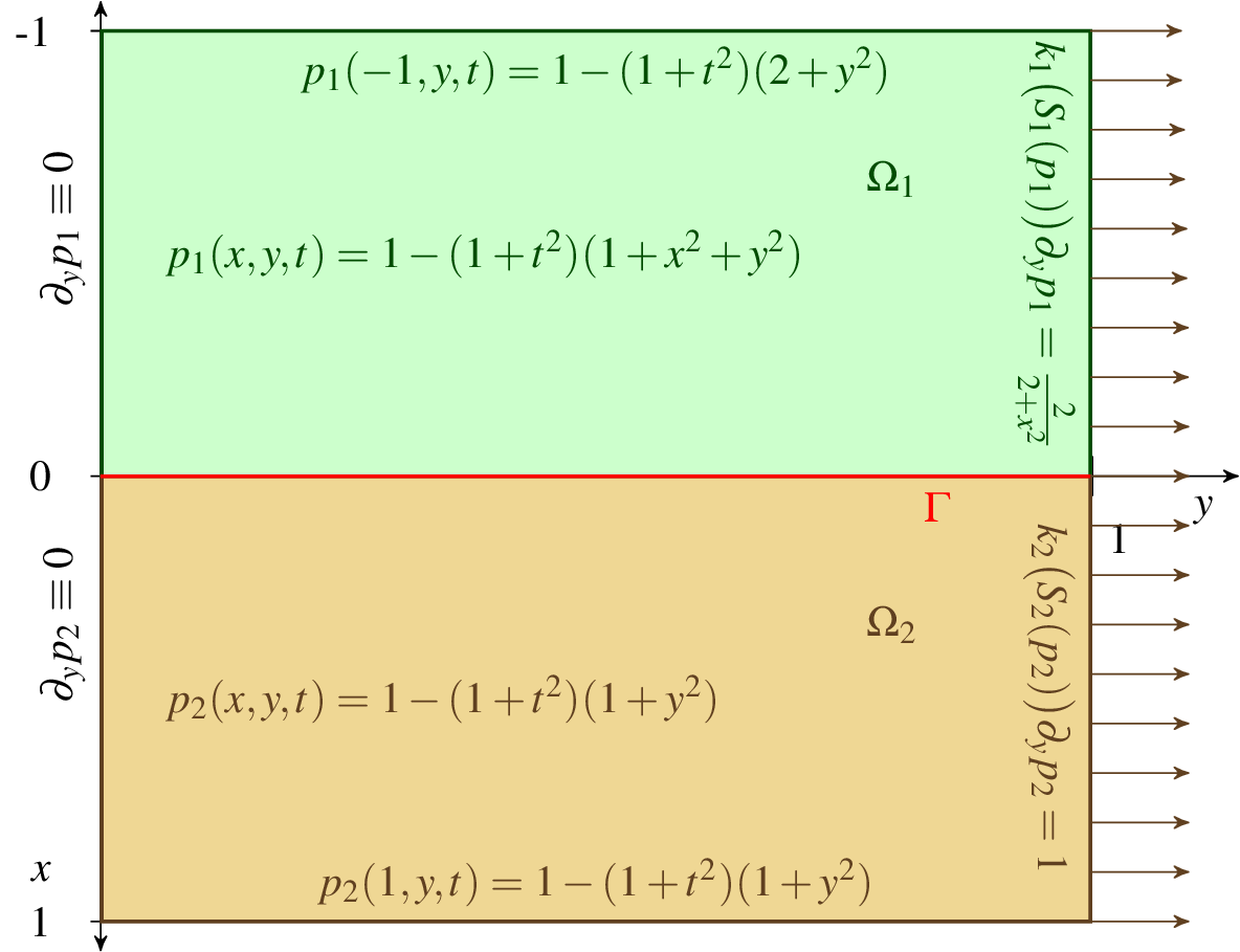
Figure 2: The domain used in the numerical examples. The boundary conditions are given in Table 1. The exact solution is also given in each subdomain.

4.1 Results for a case with known exact solution

To demonstrate the robustness of the proposed scheme, we solve (2)–(5) with both Dirichlet and Neumann type boundary conditions. In the first case we disregard gravity. Specifically, we consider

$$\Omega_{1}=(-1,0)\times(0,1),\quad\Omega_{2}=(0,1)\times(0,1),\quad\text{ and }\Gamma=\{0\}\times[0,1].$$ (57)

The relative permeabilities are $k_{1}(S_{1})=S_{1}^{2}$ on $\Omega_{1}$, $k_{2}(S_{2})=S_{2}^{3}$ on $\Omega_{2}$ and the saturations

$$S_{l}(p)=\begin{cases}\frac{1}{(1-p)^{\frac{1}{l+1}}}&\mbox{ for }p<0,\\ 1&\mbox{ for }p\geq 0\end{cases},~{}\qquad l=1,2.$$ (58)

The boundaries and right hand sides are chosen to make the exact solution

$$p_{1}(x,y,t) =1-(1+t^{2})(1+x^{2}+y^{2}), t>0,\,(x,y)\in\Omega_{1},$$

$$p_{2}(x,y,t) =1-(1+t^{2})(1+y^{2}), t>0,\,(x,y)\in\Omega_{2},$$

and this corresponds to the right hand sides

$$f_{1}(x,y,t) =\frac{4}{(1+x^{2}+y^{2})^{2}}-\frac{t}{\sqrt{(1+t^{2})^{3}(1+x^{2}+y^{2})}},$$

$$f_{2}(x,y,t) =\frac{2(1-y^{2})}{(1+y^{2})^{2}}-\frac{2t}{3\sqrt[3]{(1+t^{2})^{4}(1+y^{2})}},$$

for $t>0$, and $(x,y)\in\Omega_{l}$ respectively. The boundary and initial conditions are summed up in Table 1.

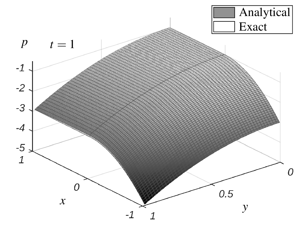
Figure 3: Comparison between the exact pressure and the numerical pressure provided by the LDD scheme.

	$\Omega_{1}$	$\Omega_{2}$
$t=0$	$p_{1}(x,y,0)=-(x^{2}+y^{2})$	$p_{2}(x,y,0)=-y^{2}$
BC$y=0$	$\partial_{y}p_{1}=0$	$\partial_{y}p_{2}=0$
$y=1$	$k_{1}\bigl{(}S_{1}(p_{1})\bigr{)}\partial_{y}p_{1}=\frac{2}{2+x^{2}}$	$k_{2}\bigl{(}S_{2}(p_{2})\bigr{)}\partial_{y}p_{2}=1$
$x=-1$	$p_{1}(-1,y,t)=1-(1+t^{2})(2+y^{2})$
$x=1$		$p_{2}(1,y,t)=1-(1+t^{2})(1+y^{2})$

Table 1: Initial and boundary conditions for the example with exact solution.

All linear systems were solved using a restarted generalised minimum residual method (gmres) [58]. To boost up speed, sparse triplet format was used in the matrix computation. The programs are implemented in ANSI C. For the implementation we took the same $L_{l}$ in both sub-domains, i.e. $L:=L_{1}=L_{2}$. The results are shown in Figures 3 and 4(a). Fig. 3 shows the pressure distribution of the exact solution $p:=\chi_{\Omega_{1}}\cdot p_{1}+\chi_{\Omega_{2}}\cdot p_{2}$ with the numerical solution $p^{n,i}:=\chi_{\Omega_{1}}\cdot p_{1}^{n,i}+\chi_{\Omega_{2}}\cdot p_{2}^{n,i}$ plotted on top of it. For $\Delta x=10^{-2}$, $\Delta t=2\cdot 10^{-4}$ as well as parameters $L=0.25$ and $\lambda=4$, the maximum relative error was less than $0.03\%$, i.e. $\bigl{\|}\tfrac{p^{n}-p^{n,i}}{p^{n}}\bigr{\|}_{L^{\infty}(\Omega)}<0.0003$. The relative errors of the LDD, LFV and Newton schemes at the mid-line $y=0.5$ are plotted in Fig. 4(a). The LDD scheme preserves the flux continuity and pressure continuity at the interface at every time step without having to solve for the entire domain. We test this theory numerically. Fig. 4(b) shows how different kinds of errors behave within one time step. The errors $\lVert p^{n,i}-p^{n,i-1}\rVert_{L^{2}(\Omega)}$, $\lVert p^{n,i}-p^{n,i-1}\rVert_{L^{\infty}(\Omega)}$ defined on the domain $\Omega$, as well as $\bigl{\|}\bigl{\llbracket}p^{n,i}\bigr{\rrbracket}\bigr{\|}_{L^{2}(\Gamma)}$ and $\bigl{\|}\bigl{\llbracket}\bm{F^{n,i}_{l}}\cdot\bm{n_{l}}\bigr{\rrbracket}\bigr{\|}_{L^{2}(\Gamma)}$ defined on the interface $\Gamma$, are shown. We observe that the flux and pressure jump tend to zero which implies that flux and pressure continuity is achieved. Note that the flux at $x=0$ from the exact solution is $0$. Next, we compare the LDD scheme with other schemes and study their dependence on discretisation parameters. We compare the Newton scheme, the (modified) Picard iteration, the already mentioned LFV scheme and the LDD scheme, investigating the dependence of time step refinement and space grid refinement separately.

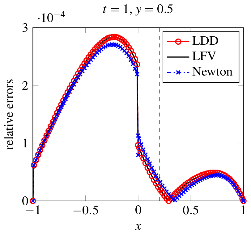
(a) Comparison between the numerical solutions provided by the LDD, LFV and the Newton schemes. Plotted are the relative errors $\bigr{\|}\frac{p_{\mbox{\tiny exact}}-p_{\mbox{\tiny num}}}{p_{\mbox{\tiny exact}}}\bigr{\|}$ as functions of $x$, for $y=0.5$ and $t=1$.

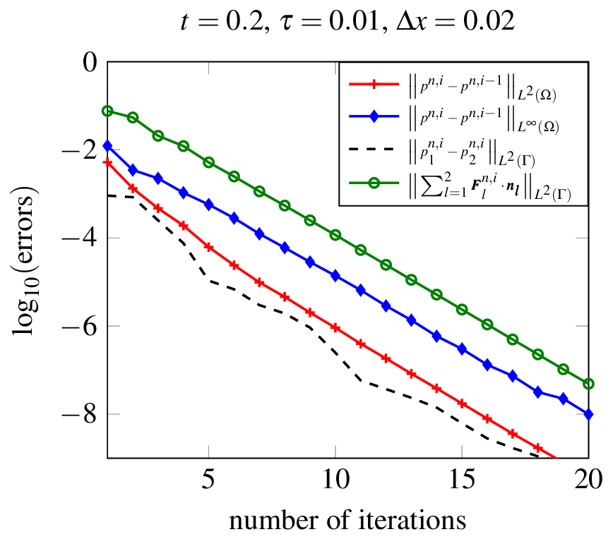
(b) Different errors vs inner iterations for the case with exact solution. Here $t=0.2$, $L=0.25$ and $\lambda=4$.

The first study, shown in Fig. 5, plots $\log_{10}\bigl{(}\|p^{n,i}-p^{n,i-1}\|_{L^{2}(\Omega)}\bigr{)}$ for all schemes, at the fixed time step corresponding to $t=0.2$. As expected, Newton is the fastest and shows a quadratic convergence rate. But at the same time, it is most susceptible to change in mesh size as observed from the slopes of the left-most curves. The convergence rate of the Picard iteration is linear, faster than both the $L$-schemes and is stable with respect to variation in mesh size. The L-schemes also exhibit linear convergence, albeit slower than Picard, and the convergence speed does not vary much with mesh size. LFV and LDD schemes have practically the same convergence rate. Table 2 complements the plot in Fig. 5 and lists experimental average convergence rates, defined as $\|e^{n,i+1}_{p}\|/\|e^{n,i}_{p}\|$, for all schemes (Newton data is not shown for $\Delta x=0.1$, $0.05$, $0.02$ as it reaches an error lower than $10^{-10}$ in 3 iterations).

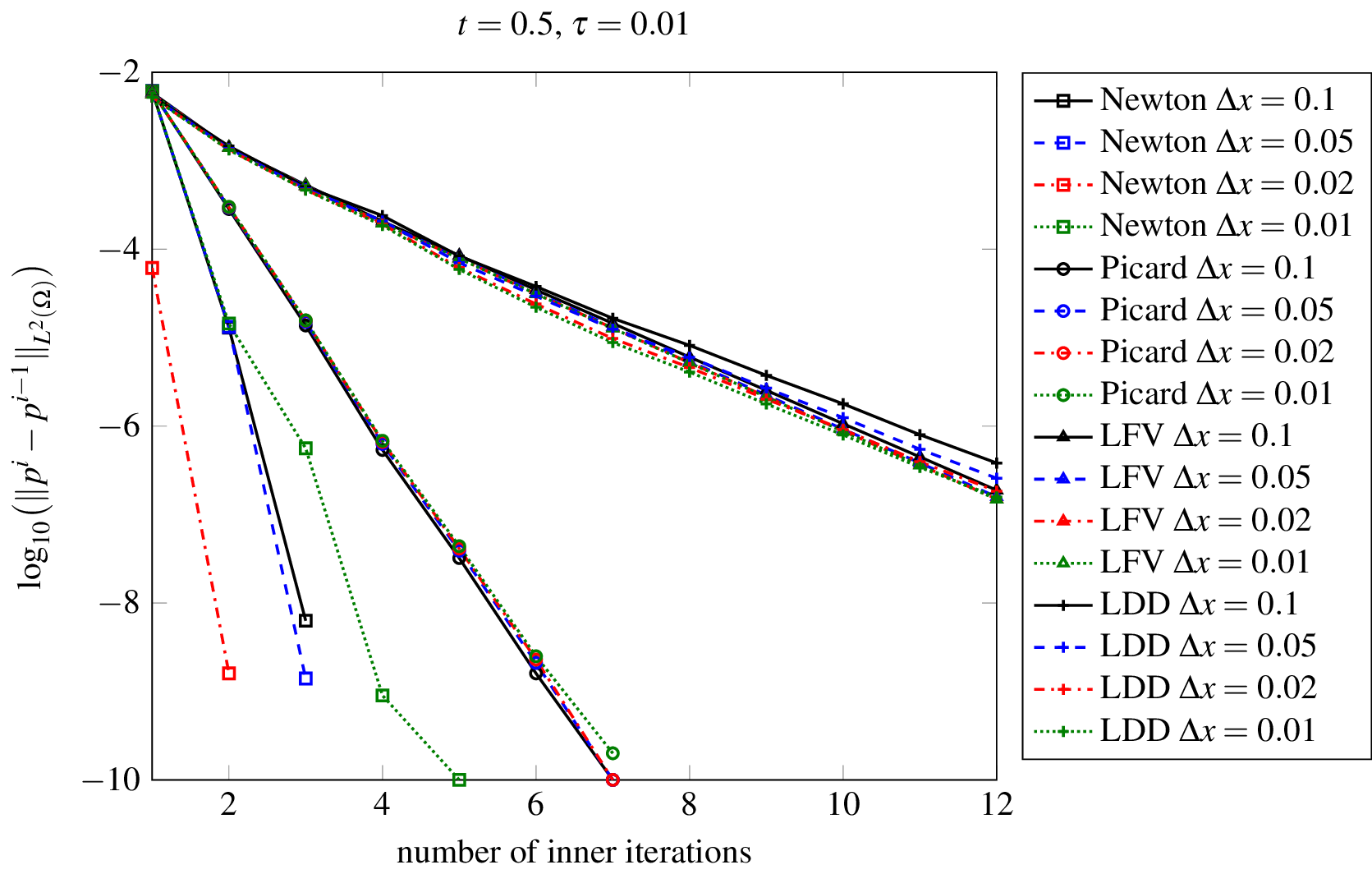
Figure 5: Performance comparison and mesh study for the convergence of the LDD, LFV, Picard and Newton schemes. Here $L=0.25$ and $\lambda=4$.

$\Delta x$	Newton	Picard	LFV	LDD
$0.1$	-	0.0504	0.4046	0.4400
$0.05$	-	0.0504	0.3906	0.4270
$0.02$	-	0.0505	0.3909	0.4221
$0.01$	0.0113	0.0567	0.3910	0.4221
Type	Quadratic	Linear	Linear	Linear

Table 2: The average convergence rate, $\|e^{n,i+1}\|/\|e^{n,i}\|$, for the different schemes and with respect to the mesh-size.

Secondly, we study the dependence of the convergence rates on time step size for a fixed mesh size ($\Delta x=0.02$). The error characteristics of all four schemes in Fig. 6 are shown for $t=0.5$. In Fig. 6(a) both, Newton and Picard, diverge, whereas both $L$-schemes converge for $L=0.25$. The LFV scheme exhibits some oscillations, the reason being the dependence of the choice of $L$ on the time step $\tau$. Higher values of $\tau$ might require higher values of $L$. Indeed, if we substitute $L=0.5$ in the LFV scheme (marked as LFV* in the diagram), we see a more robust behaviour. Note, that the LDD scheme converges for all $\tau$ and is at least as fast as the LFV scheme in all the cases. For smaller values of $\tau$ the Newton and Picard iteration converge faster than both L-schemes, as shown in Figures 6(b) and 6(c).

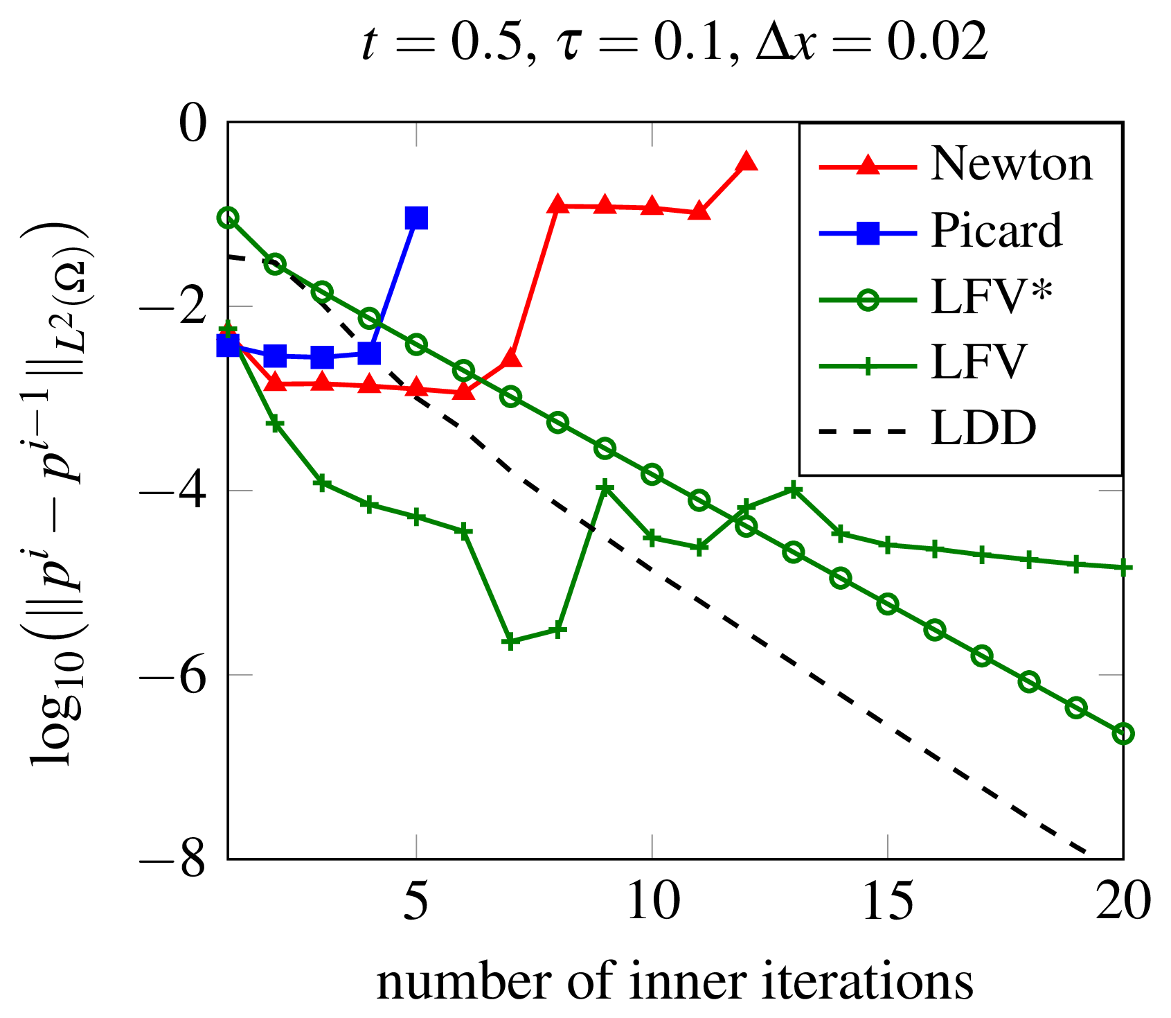
(a) $\Delta t=0.1$

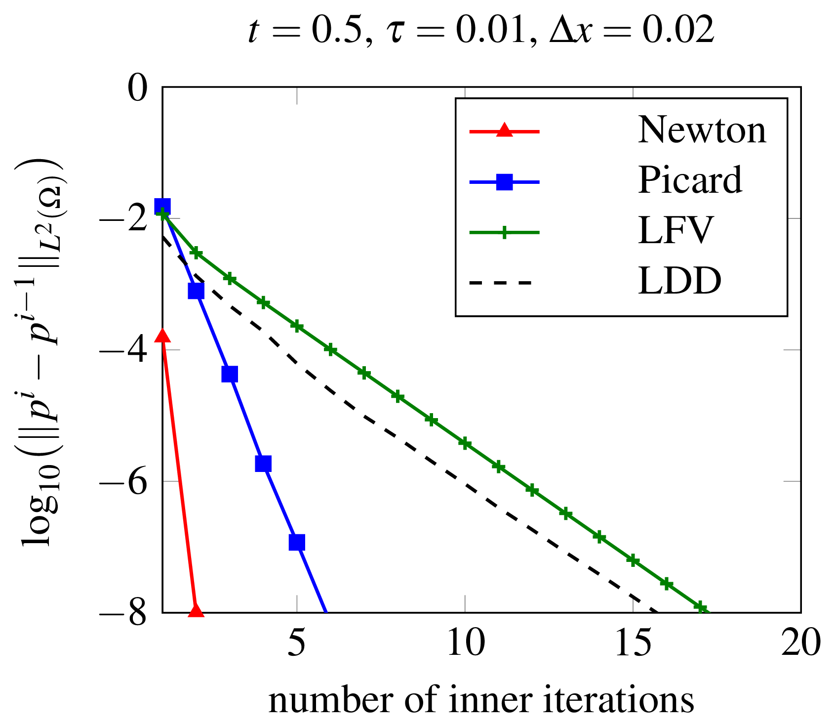
(b) $\Delta t=0.01$

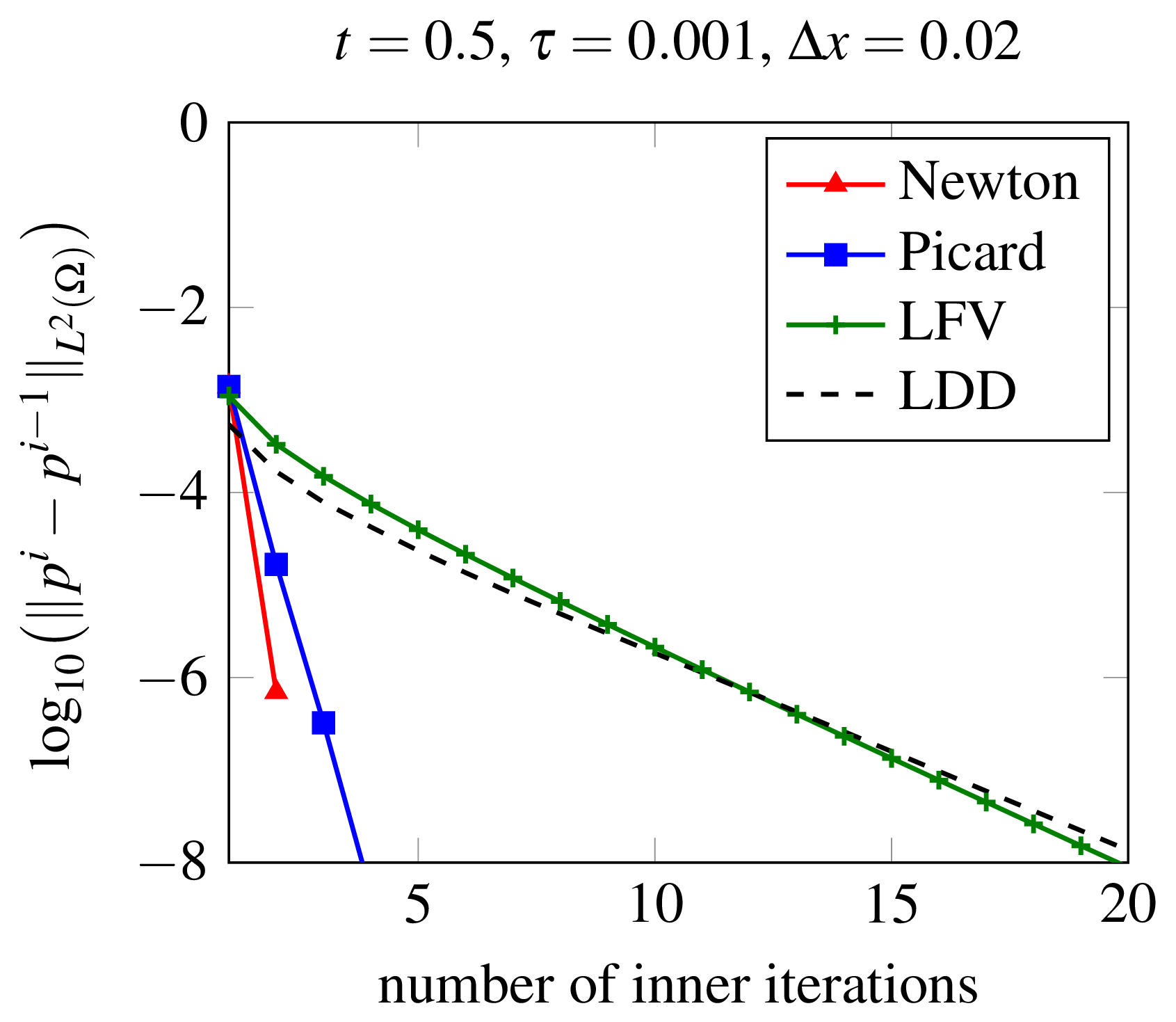
(c) $\Delta t=0.001$

Figure 6: Convergence study for the time-steps $\tau=0.1$, $0.01$, $0.001$. Here, $L=0.25$ for the LFV scheme and $L=0.5$ for the LFV* scheme. For the LDD scheme one has $L=0.25$, $\lambda=2$ in case 6(a), $L=0.25$, $\lambda=4$ in case 6(b), and $L=0.25$, $\lambda=10$ in case 6(c).

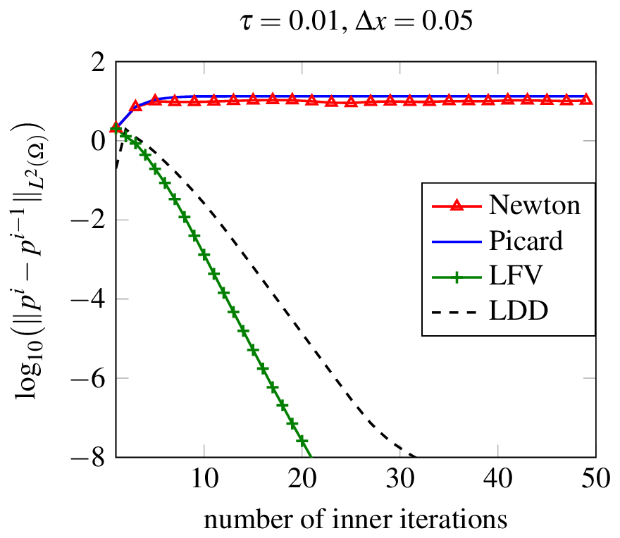
Figure 7: Error decay for the different schemes for a constant initial guess, $p^{n,0}=-5$. Here $L=0.25$, $\lambda=4$.

According to the theory, the convergence of the Newton and Picard schemes is only guaranteed if the initial guess is close enough to the exact solution. Therefore, starting the iteration with the numerical solution at the previous time step this suggests that the time step should be taken small enough to have a guaranteed convergence (see [24, 30, 33]. Contrariwise, L-schemes are free of this constraint.

To illustrate this behaviour, we have investigated the convergence of the schemes for a constant initial guess. Specifically, $p^{n,0}=-5$ has been used instead of $p^{n,0}=p^{n-1}$. In this case, the Newton and Picard schemes are divergent whereas both L-schemes still produce a good approximation after several iterations. This is displayed in Fig. 7. A similar behaviour will be observed again while discussing a numerical example with realistic parameters.

Remark 10.

The convergence behaviour of the LDD scheme can be optimized by choosing $\lambda$ properly. In the above comparison $\lambda$ was chosen differently for every choice of mesh size. The optimality of $\lambda$ is dependent on the mesh and the time step size. With a good choice of $\lambda$, one can make the LDD scheme at least as fast as the LFV scheme. This is discussed in more detail in Section 4.3.

4.1.1 Results for a realistic case with van Genuchten parameters

We demonstrate the applicability of the LDD scheme for a case with realistic parameters, incorporating also gravity effects. We consider a van-Genuchten-Mualem parametrisation [59] with the curves $k$ and $S$

$$S_{l}(p) =S_{l,r}+(S_{l,s}-S_{l,r})\Phi_{l}(p),$$ (59)

$$\Phi_{l}(p) =\dfrac{1}{\bigl{(}1+(-\alpha_{l}p)^{\hat{n}_{l}}\bigr{)}^{m_{l}}},\qquad m_{l}=1-\dfrac{1}{\hat{n}_{l}},$$

$$k_{l}(S) =\sqrt{\Phi_{l}(p)}\Bigl{(}1-\bigl{(}1-\Phi_{l}(p)^{\frac{1}{m_{l}}}\bigr{)}^{m_{l}}\Bigr{)}^{2}.$$

The specific parameter values are listed in Table 3 and are characteristic for particular types of materials, silt loam G.E. 3 ($\Omega_{1}$) and sandstone ($\Omega_{2}$). These materials have very different absolute permeabilities $\kappa_{1},\kappa_{2}$, which makes the numerical calculations more challenging.

The dimensional governing equations and boundary conditions become ($l=1,2$)

$$L_{l}p_{l}^{n,i}+\tau\nabla \cdot\bm{F_{l}^{n,i}}=L_{l}p_{\ell}^{n,i-1}$$

$$-\phi_{l}\bigl{(}S_{l}(p_{l}^{n,i-1})-S_{l}(p_{l}^{n-1})\bigr{)}, \text{ on }\Omega_{l},$$ (60)

$$\bm{F_{l}^{n,i}}\cdot\bm{n_{l}} =g^{i}_{l}+2\lambda p_{l}^{n,i}, \text{ on }\Gamma,$$ (61)

$$p_{l}^{n,i}, =0 \text{ on }\partial\Omega_{l}.$$ (62)

In this case $\bm{F_{l}^{n,i}}=-\frac{\kappa_{l}}{\mu}k_{r,l}\bigl{(}S_{l}(p_{l}^{n,i-1})\bigr{)}\bigl{(}\bm{\nabla}p_{l}^{n,i}-\rho\bm{g}\bigl{)}$. Here $\bm{g}=g\bm{e_{x}}$ is the gravitational acceleration aligned with the positive $x$-direction, $\rho$, $\mu$ are the density and the viscosity of the fluid and $\kappa_{l}$, $\phi_{l}$ are the absolute permeability as well as the porosity of the medium. Note that Fig. 2 is rotated by 90 degrees.

Parameter	Unit	Silt Loam G.E. 3 $(\Omega_{1})$	Sandstone $(\Omega_{2})$
Porosity ($\phi_{l}$)	-	$0.35$	$0.35$
Water Density ($\rho$)	kg m-3	$1\times 10^{3}$	$1\times 10^{3}$
Water Viscosity ($\mu$)	Pa$\cdot$s	$1\times 10^{-3}$	$1\times 10^{-3}$
Absolute permeability ($\kappa_{l}$)	m2s	$5.7407\times 10^{-14}$	$1.2500\times 10^{-12}$
Retention exponent ($\hat{n}_{l}$)	-	$2.06$	$10.4$
Retention parameter ($\alpha_{l}$)	Pa-1	$4.23\times 10^{-5}$	$7.90\times 10^{-5}$
Irreducible water saturation ($S_{l,r}$)	-	$0.131$	$0.153$
Irreducible air saturation ($1-S_{l,s}$)	-	$0.604$	$0.75$

Table 3: The van Genuchten-Mualem parameters in the realistic test case.

The problem is nondimensionalised by using the characteristic pressure $p^{*}:=-14.8\times 10^{3}$Pa, length $1.48$m and time $41.440$s. This leads to the nondimensional quantities $\tilde{p}$, $(x,y)$ and $t$. After nondimensionalisation, the domain used is again taken to be $\Omega_{1}=(-1,0)\times(0,1)$, $\Omega_{2}=(0,1)\times(0,1)$. The initial condition used is

$$\tilde{p}(x,y,0)=-1$$ (63)

and boundary conditions are

$$\tilde{p}(-1,y,t)=\begin{cases}-1+ty&\text{ if }y<(1-\epsilon)t^{-1}\\ -\epsilon&\text{ if }y\geq(1-\epsilon)t^{-1}\end{cases},$$

$$\tilde{p}(1,y,t)=-1,$$

together with a no-flow condition at $y=0,1$. We take $\epsilon>0$ to avoid degeneracy.

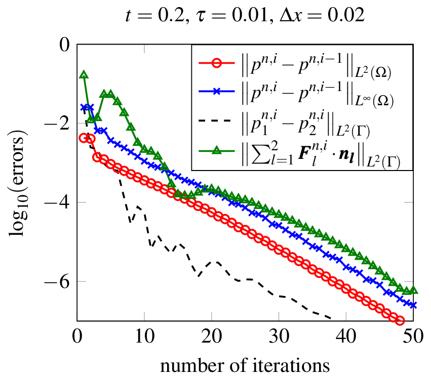
(a) Different errors vs inner iterations for the realistic case at $t=0.2$. The parameters are $\tau=0.01$, $\Delta x=0.02$, $L_{l}=0.25$ and $\lambda=10$. Only the LDD scheme is shown in this plot.

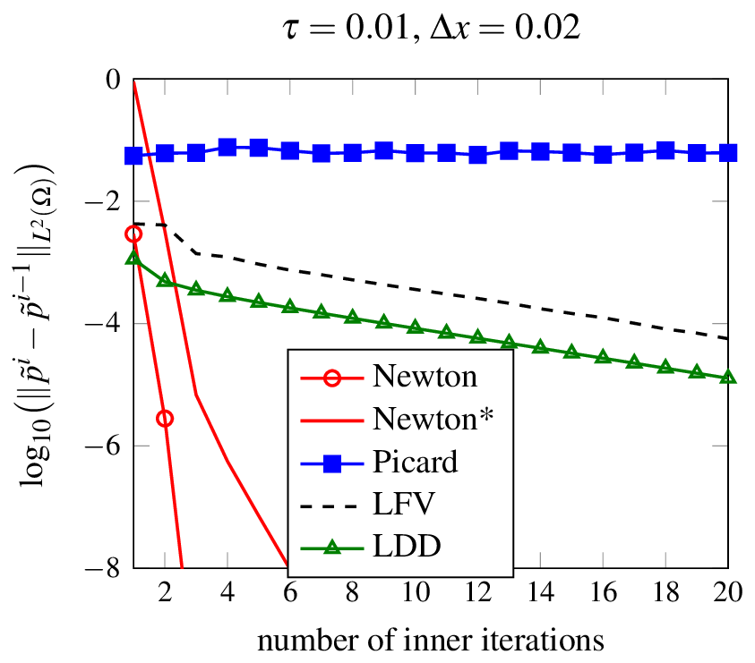
(b) Error vs inner iterations for the realistic case. LDD , LFV and Newton errors are plotted at $t=0.2$. Newton^∗ denotes the errors of Newton scheme at $t=0.9$. Picard is plotted at $t=0.02$. Here, $L=0.5$, $\lambda=10$.

Figure 8: Error plots and scheme comparison for the realistic case.

Fig. 8(a) shows the different errors for this case and it can be seen that all the errors are decreasing for the LDD scheme. Errors at the interface and inside the domain tend to $0$, the convergence is slower compared to the case with exact solution, however. This is due to the large variance of the parameters as well as the highly nonlinear nature of the associated functions. Because of this, both Newton and Picard schemes diverge. The behaviour of different schemes for the same set of parameters is shown in Fig. 8(b). Observe that for the Newton scheme the starting error as well as the number of iterations required increases steadily with $t$ until $t=0.94$, at which point the errors start diverging. The Picard scheme becomes divergent even before $t=0.2$. In contrast, both L-schemes remain stable in this case.

4.2 Time Performance

This section is devoted to the comparison of time performance of the schemes. We have seen that L-schemes are more stable than Newton and Picard. But if they are converging, then Newton and Picard schemes converge faster than the L-schemes. Below we investigate how the schemes compare to one another with respect to actual computational time. We set an error tolerance for the schemes that stops the iterations within one time step, after reaching an error lower than $10^{-6}$, i.e. $\lVert p^{n,i}-p^{n,i-1}\rVert_{L^{2}(\Omega)}<10^{-6}$. This is to ensure that we get comparative CPU-clock-time for different schemes for the same degree of accuracy.

Condition number
$\Delta x$	0.1	0.05	0.02
L-DD ($\Omega_{1}$)	7.6191	11.8947	73.362
L-DD ($\Omega_{2}$)	7.0219	12.3557	74.519
L-FV ($\Omega$)	94.8158	171.47	397.34

Table 4: The condition number vs mesh size for the LDD and LFV schemes. Here, $\tau=0.001$, $t=0.2$, $L=0.25$, $\lambda=10$. The condition numbers are calculated for the $200^{th}$ time step for the matrices of the first inner iteration.

We computed the exactly solvable case on a LINUX server (mammoth.win.tue.nl) for all four schemes using the same set of parameters ($\Delta x=0.02$, $\tau=0.001$, $L=0.25$ and $\lambda=10$). Figure 9 illustrates the time-performances of these schemes over the whole computational time domain. Table 5 shows how many inner-iterations are required on average for different schemes to reach the error criterion at different points in time.

Iteration requirement per time step increases for all schemes as the boundary conditions change more rapidly with time. Table 5 shows the average time taken and how many gmres iterations (outer and inner) were required by each scheme to execute one inner iteration.

Unsurprisingly, the Newton scheme is still fastest, followed by Picard and the LDD scheme. But LDD competes closely with Newton and Picard. Even more surprising is the fact that the LFV scheme takes

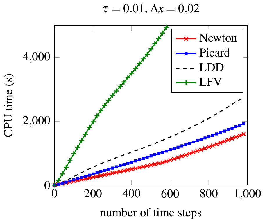
Figure 9: Time performance of the L-DD, L-FV and the Newton-FV schemes.

considerably more time to reach the desired accuracy compared to the LDD scheme, despite both having almost the same convergence rate. The reason becomes apparent from Table 5: The LDD scheme requires much less time per inner iteration than all other schemes. The LFV scheme has the second fastest average time per iteration. For the Picard iteration, the derivative of the saturation function needs to be evaluated which in turn costs more time than an iteration in the LFV scheme. The Newton scheme is computationally most expensive per iteration because it calculates the Jacobian at every iteration.

Average inner iterations required
Time-step/Scheme	LDD	LFV	Picard	Newton
10	7.3	7.5	2.3	2.3
50	9.880	10.72	2.520	2.060
100	11.26	12.31	2.760	2.030
500	11.19	11.79	2.952	2.006
1000	14.18	14.35	2.946	2.408
Avg. time per iter.	0.1965	0.5392	0.6591	0.6722
Avg. GMRES iterations	119+ 123	396.6	390.9	397.7

Table 5: The average number of inner iterations per time step required by the different schemes to reach the stopping criterion $\lVert p^{n,i}-p^{n,i-1}\rVert_{L^{2}(\Omega)}<10^{-6}$. The last two rows give the average time and gmres-iterations per inner iteration.

The schemes that do not decouple the domain require much more time and many more gmres-iterations per inner iteration. The reason is that the domain decomposition schemes involve smaller matrices and and they have smaller condition numbers. This is illustrated by the last row of Table 5. The LDD scheme requires on average 119 gmres-iterations on $\Omega_{1}$ and 123 gmres-iterations on $\Omega_{2}$ and both domains have $52\times 50$ elements. Compare this with Newton, which takes almost 400 gmres-iterations and deals with $104\times 50$ variables on each gmres-iteration. This explains why the LDD scheme takes so much less time per inner iteration. Table 4 compares the condition numbers of the LDD and the LFV scheme. It shows that the matrices for the LFV scheme are worse conditioned than the ones of the LDD scheme. The latter has two condition numbers, one for each domain. The 2-norm condition numbers were calculated with MATLAB’s build in cond() function.

Remark 11.

The fact that the LDD scheme performance competes closely with Newton and Picard, means that, LDD can potentially be made much faster than even Newton as it is parallelisable. This is the key advantage of the LDD scheme along with its global convergence property.

4.3 Parameter dependence and key features

Having outlined the robustness and speed of the proposed LDD scheme we turn to investigate some of its properties. Two important parameters have been introduced in the L-DD scheme, i.e. $L_{l}$ and $\lambda$, and apart from a lower bound on $L_{l}$ nothing has been specified about these parameters. This means that they can freely be adjusted to give optimal convergence rate. In fact, in this section we will see that the convergence rate depends strongly on these parameters.

The influence of $\lambda$

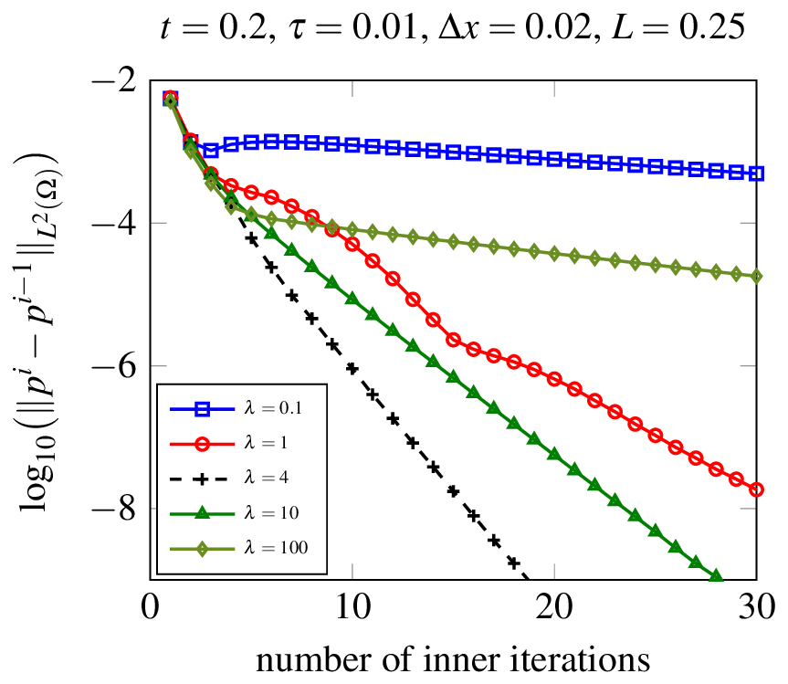
(a) The decay of the pressure error in terms of $\lambda$.

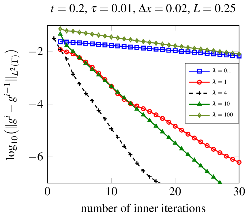
(b) The decay of the $g$-error in terms of $\lambda$.

Figure 10: The influence of $\lambda$ on the convergence rate. The parameters for the LDD scheme are $\tau=.01$, $\Delta x=0.02$, $L_{l}=0.25$ at $t=0.2$.

Figure 10 shows the influence of the parameter $\lambda$ on error characteristics. All the results shown are for the case with exact solution. Figure 10(a) focuses on the errors $\lVert p^{n,i}-p^{n,i-1}\rVert_{L^{2}(\Omega)}$

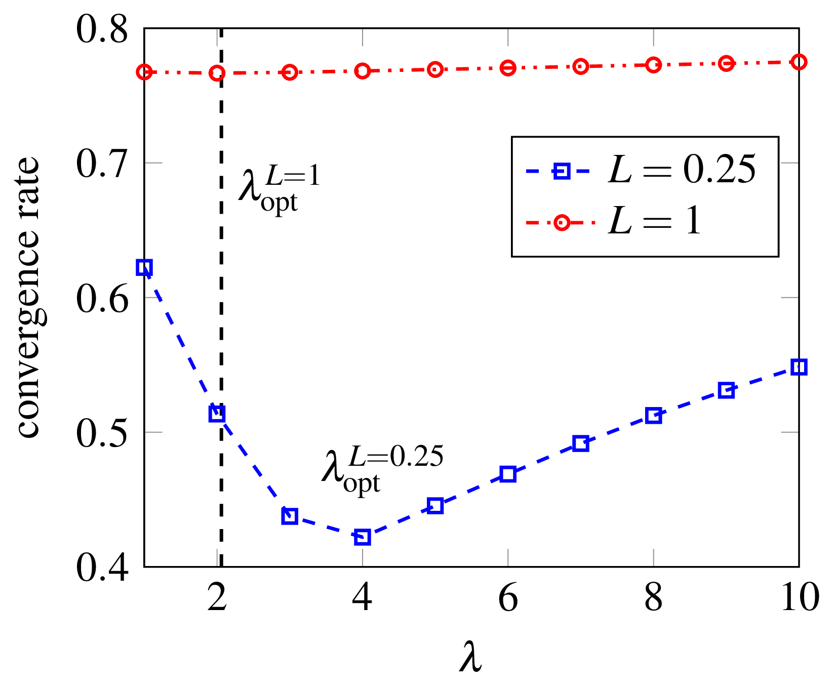
Figure 11: Convergence rate vs $\lambda$ for $L=0.25$ and $L=1$. For $L=0.25$, $\lambda_{\mbox{\scriptsize opt}}\approx 4$.

on the domain $\Omega$, while Fig. 10(b) depicts the $L^{2}$-errors $\lVert g^{i}-g^{i-1}\rVert_{L^{2}(\Gamma)}$ on the interface for the same time step. Clearly, $\lambda$ has tremendous impact on the convergence rate. The convergence rate rapidly increases with $\lambda$ at first but after a certain point the convergence rate starts decreasing. This trend is noticeable in both plots of Figure 10. This indicates that there is an optimal lambda $\lambda_{\mbox{\scriptsize opt}}$ for which the whole scheme has a fastest convergence rate. The optimality of $\lambda$ is actually a well studied behaviour in the domain decomposition literature. In [60, 50] it has been shown that $\lambda_{opt}$ depends at least on mesh size and sub- domain size. Later we will show that it also depends on $L_{l}$ and $\tau$ in our case. This control over the convergence rate is the reason why the $\lambda$-formulation was chosen over the convex-combination formulation given in Remark 2. To illustrate this, Fig. 12 shows the same plots as Figure 10 but for the convex-combination formulation. In order to differentiate between plots more easily, we use the combined formulation (11’’), (12’’) and set $M=1$. For $\eta=0.01$ the convex-combination formulation even fails to converge. In all other cases the convergence is considerably slower.

(a) The decay of the pressure error in terms of $\eta.$

(b) The decay of the $g$-error in terms of $\eta.$

Figure 12: The influence of $\eta$ on the convergence rate in the convex-combination formulation ($M=1$ in Remark 2). The parameters for the LDD scheme are $\tau=0.01$, $\Delta x=0.02$, $L_{l}=0.25$ at $t=0.2$.

The influence of $L_{l}$

Figure 13: The influence of $L$ on the convergence rate, as obtained for the inner iterations for the $50^{th}$ time step.

We briefly give an overview over the influence of $L_{l}$ on the convergence rate. Figure 13 depicts this for $L:=L_{1}=L_{2}$. For L-schemes it is common to diverge if $L$ is too small, which seems to be the case for $L=0.1$. On the other hand, the convergence rate decreases significantly for very large $L$, a behaviour that is a common trait of L-schemes as well, cf. [10]. It is best to choose $L$ as small as possible, yet great enough to ensure convergence of the scheme. Note that $L_{l}=0$ represents the original (nonmodified) Picard iteration case and Figure 13 suggests that the original Picard scheme fails for these problems.

The dependence of $\lambda_{\mbox{\scriptsize opt}}$ on $L_{l}$, $\tau$ and $\Delta x$

In this last section we investigate numerically how $\lambda_{\mbox{\scriptsize opt}}$ depends on the choice of $L$, $\tau$ and $\Delta x$. For a fixed grid in time and space Table 6 lists convergence rates for different $\lambda$ and $L$. With this table we can guess the interval in which $\lambda_{\mbox{\scriptsize opt}}$ lies. Within this estimated interval, Fig. 11 shows how the convergence rate varies with $\lambda$ for fixed $L$. For $L=0.25$, $\Delta x=0.02$ and $\tau=0.01$ the fastest convergence is achieved for $\lambda=4$ (this is why $\lambda=4$ was chosen for the above comparisons, wherever the specified $L$, $\Delta x$, $\tau$ set was used). The $\lambda$ dependence for higher values of $L$ is less pronounced.

For a fixed $L$, Tables 7(a), 7(b) show the variance of $\lambda_{\mbox{\scriptsize opt}}$ with respect to time-step and mesh size respectively. The shown tables are of course only a rough estimate of $\lambda_{\mbox{\scriptsize opt}}$. Due to computation time, it is a tedious process to find a close to exact value of $\lambda_{\mbox{\scriptsize opt}}$, especially for very small time-step sizes. In practice the values are numerically guessed. The results indicate quite a strong correlation of $\lambda_{\mbox{\scriptsize opt}}$ with the time-step size, contrasted by a rather minor correlation with the mesh size.

$L$	$\lambda=0.1$	$\lambda=1$	$\lambda=10$	$\lambda=100$	$\lambda_{\mbox{\scriptsize opt}}\in$
0.1	diverged	diverged	diverged	diverged	-
0.25	0.9020	0.6223	0.5480	0.7721	($1$,$10$)
1	diverged	0.7675	0.7750	0.8138	($1$,$10$)
5	diverged	0.8993	0.8718	0.8708	($10$,$100$)

Table 6: The dependence of the convergence rates on $\lambda$ and $L$: the geometric average of the contraction rates over the first 20 iterations and for different $(L,\lambda)$ pairs is given in the first columns, whereas the last gives the interval for $\lambda_{\mbox{\scriptsize opt}}$. Here, $\Delta x=0.02$, $\Delta t=0.01$, $t=0.2$.

$\Delta t$	0.1	0.01	0.001
Nr iter.?	2	4	6
Avg. CR	0.4444	0.4221	0.5408

(a) $\lambda_{\mbox{\scriptsize opt}}$ for $\Delta x=0.02$, $L_{l}=0.25$

$\Delta x$	0.1	0.05	0.02	0.01
Nr iter.?	3	4	4	4
Avg. CR	0.4398	0.4270	0.4221	0.4221

(b) $\lambda_{\mbox{\scriptsize opt}}$ for $\Delta t=0.01$, $L_{l}=0.25$

Table 7: The dependence of $\lambda_{\mbox{\scriptsize opt}}$ on $\Delta t$ and on $\Delta x$.

5 Conclusion

We considered a nonlinear parabolic problem appearing as mathematical model for variably saturated flow in porous media. For the numerical solution of the nonlinear, time discrete problems we proposed a combined scheme ($LDD$) that is based on a fixed point iteration (the $L$-scheme), and on a domain decomposition scheme involving Robin type coupling conditions at the interface separating different subdomains. The result is a scheme featuring the advantages of both approaches: an unconditional convergence, regardless of time step and starting point, as well as a decoupling of the time discrete problems into subproblems that can be solved in parallel. The stability, robustness and efficiency of the method is tested for various cases and also compared to Newton and Picard schemes. The tests include situations where the latter diverge whereas the proposed scheme is converging. In summary, the key advantages of the method are:

• The LDD scheme converges unconditionally. It can provide accurate results even in situations where the Picard or Newton iterations fail.

• In conjunction with a suitable space discretisation, it provides a decoupled, mass conservative approach. This is very useful in particular when dealing with models defined in media with block-type heterogeneities, where the material properties in different blocks may vary significantly.

• Though linearly convergent, the computational time required by the LDD scheme for achieving a certain accuracy of the approximation is comparable to the time needed by Newton and Picard schemes, and much faster than a standard L-scheme applied to the model in the entire domain. This efficiency is due to the fact that the scheme needs less time per inner iteration than a scheme defined in the entire domain. Moreover LDD is parallelisable, which gives the possibility of increasing its efficiency even further.

• The convergence rate of LDD schemes depends on the choice of $L$ and $\lambda$. With the optimal choice of parameters, the convergence order can be reduced significantly.

References

- [1] R. Helmig, Multiphase flow and transport processes in the subsurface: a contribution to the modeling of hydrosystems, Springer, Berlin, 1997.
- [2] L. F. Richardson, Weather prediction by numerical process, Camebridge University Press, 1922.
- [3] L. A. Richards, Capillard conduction of liquids through porous mediums, Physics 1 (5) (1931) 318–333.
- [4] H. W. Alt, S. Luckhaus, Quasilinear elliptic-parabolic differential equations, Math. Z. 183 (3) (1983) 311–341.
- [5] H. W. Alt, S. Luckhaus, A. Visintin, On nonstationary flow through porous media, Annali di Matematica Pura ed Applicata 136 (1) (1984) 303–316.
- [6] F. Otto, L1-contraction and uniqueness for quasilinear elliptic–parabolic equations, Journal of Differential Equations 131 (1) (1996) 20–38.
- [7] T. Arbogast, M. F. Wheeler, A Nonlinear Mixed Finite Element Method for a Degenerate Parabolic Equation Arising in Flow in Porous Media, SIAM J. Numer. Anal. 33 (4) (1996) 1669–1687.
- [8] R. H. Nochetto, C. Verdi, Approximation of degenerate parabolic problems using numerical integration, SIAM J. Numer. Anal. 25 (4) (1988) 784–814.
- [9] I. S. Pop, Error estimates for a time discretization method for the Richards’ equation, Comput. Geosci. 6 (2) (2002) 141–160.
- [10] F. A. Radu, I. S. Pop, P. Knabner, Order of Convergence Estimates for an Euler Implicit, Mixed Finite Element Discretization of Richards’ Equation, SIAM J. Numer. Anal. 42 (4) (2004) 1452–1478.
- [11] F. A. Radu, I. S. Pop, P. Knabner, Error estimates for a mixed finite element discretization of some degenerate parabolic equations, Numerische Mathematik 109 (2) (2008) 285–311.
- [12] F. A. Radu, K. Kumar, J. M. Nordbotten, I. S. Pop, A robust, mass conservative scheme for two-phase flow in porous media including Hölder continuous nonlinearities, IMA Journal of Numerical Analysis (2017) pages t.b.a.
- [13] R. A. Klausen, F. A. Radu, G. T. Eigestad, Convergence of MPFA on triangulations and for Richards’ equation, Int. J. Numer. Methods Fluids 58 (12) (2008) 1327–1351.
- [14] I. Yotov, A mixed finite element discretization on non–matching multiblock grids for a degenerate parabolic equation arizing in porous media flow, East–West J. Numer. Math. 5 (1997) 211–230.
- [15] C. S. Woodward, C. N. Dawson, Analysis of expanded mixed finite element methods for a nonlinear parabolic equation modeling flow into variably saturated porous media, SIAM J. Numer. Anal. 37 (3) (2000) 701–724.
- [16] M. Slodička, A Robust and Efficient Linearization Scheme for Doubly Nonlinear and Degenerate Parabolic Problems Arising in Flow in Porous Media, SIAM J. Sci. Comput. 23 (5) (2002) 1593–1614.
- [17] H. Berninger, R. Kornhuber, O. Sander, Fast and Robust Numerical Solution of the Richards Equation in Homogeneous Soil, SIAM J. Numer. Anal. 49 (6) (2011) 2576–2597.
- [18] P. Bastian, O. Ippisch, F. Rezanezhad, H. J. Vogel, K. Roth, Numerical Simulation and Experimental Studies of Unsaturated Water Flow in Heterogeneous Systems, Springer Berlin Heidelberg, Berlin, Heidelberg, 2007, pp. 579–597.
- [19] Y. Epshteyn, B. Rivière, Analysis of hp discontinuous galerkin methods for incompressible two-phase flow, J. Comput. Appl. Math. 225 (2) (2009) 487–509.
- [20] R. Eymard, M. Gutnic, D. Hilhorst, The finite volume method for Richards equation, Comput. Geosci. 3 (3) (1999) 259–294.
- [21] R. Eymard, D. Hilhorst, M. Vohralík, A combined finite volume–nonconforming/mixed-hybrid finite element scheme for degenerate parabolic problems, Numerische Mathematik 105 (1) (2006) 73–131.
- [22] M. Bause, P. Knabner, Computation of variably saturated subsurface flow by adaptive mixed hybrid finite element methods, Adv. Water Resour. 27 (6) (2004) 565 – 581.
- [23] L. Bergamaschi, M. Putti, Mixed finite elements and Newton-type linearizations for the solution of Richards’ equation, Int. J. Numer. Methods Eng. 45 (8) (1999) 1025–1046.
- [24] E.-J. Park, Mixed finite element methods for nonlinear second-order elliptic problems, SIAM J. Numer. Anal. 32 (3) (1995) 865–885.
- [25] K. Brenner, C. Cancès, Improving newton’s method performance by parametrization: The case of the richards equation, SIAM Journal on Numerical Analysis 55 (4) (2017) 1760–1785.
- [26] M. A. Celia, E. T. Bouloutas, R. L. Zarba, A General Mass-Conservative Numerical Solution for the Unsaturated Flow Equation, Water Resour. Res. 26 (7) (1990) 1483–1496.
- [27] P. Lott, H. Walker, C. Woodward, U. Yang, An accelerated Picard method for nonlinear systems related to variably saturated flow, Adv. Water Resour. 38 (2012) 92 – 101.
- [28] W. Jäger, J. Kačur, Solution of doubly nonlinear and degenerate parabolic problems by relaxation schemes, ESAIM: Mathematical Modelling and Numerical Analysis - Modélisation Mathématique et Analyse Numérique 29 (5) (1995) 605–627.
- [29] J. Kačur, Solution to strongly nonlinear parabolic problems by a linear approximation scheme, IMA Journal of Numerical Analysis 19 (1) (1999) 119–145.
- [30] F. A. Radu, I. S. Pop, P. Knabner, On the convergence of the Newton method for the mixed finite element discretization of a class of degenerate parabolic equation, Numerical Mathematics and Advanced Applications (2006) 1194–1200.
- [31] I. S. Pop, F. A. Radu, P. Knabner, Mixed finite elements for the Richards’ equation: linearization procedure, J. Comput. Appl. Math. 168 (1–2) (2004) 365–373.
- [32] F. A. Radu, J. M. Nordbotten, I. S. Pop, K. Kumar, A robust linearization scheme for finite volume based discretizations for simulation of two-phase flow in porous media, J. Comput. Appl. Math. 289 (2015) 134–141.
- [33] F. List, F. A. Radu, A study on iterative methods for solving Richards’ equation, Comput. Geosci. 20 (2) (2016) 341–353.
- [34] A. Quarteroni, A. Valli, Domain decomposition methods for partial differential equations, repr. Edition, Numerical mathematics and scientific computation, Clarendon Press, Oxford [u.a.], 2005.
- [35] V. Dolean, P. Jolivet, F. Nataf, An introduction to domain decomposition methods, Society for Industrial and Applied Mathematics (SIAM), Philadelphia, PA, 2015, algorithms, theory, and parallel implementation.
- [36] R. Glowinski, Q. V. Dinh, J. Periaux, Domain decomposition methods for nonlinear problems in fluid dynamics, Comput. Methods Appl. Mech. Engrg. 40 (1) (1983) 27–109.
- [37] M. Dryja, W. Hackbusch, On the nonlinear domain decomposition method, BIT 37 (2) (1997) 296–311.
- [38] X.-C. Tai, M. Espedal, Rate of convergence of some space decomposition methods for linear and nonlinear problems, SIAM J. Numer. Anal. 35 (4) (1998) 1558–1570.
- [39] J. O. Skogestad, E. Keilegavlen, J. M. Nordbotten, Domain decomposition strategies for nonlinear flow problems in porous media, J. Comput. Phys. 234 (2013) 439–451.
- [40] J. O. Skogestad, E. Keilegavlen, J. M. Nordbotten, Two-scale preconditioning for two-phase nonlinear flows in porous media, Transp. Porous Media 114 (2) (2016) 485–503.
- [41] M. J. Gander, O. Dubois, Optimized Schwarz methods for a diffusion problem with discontinuous coefficient, Numer. Algorithms 69 (1) (2015) 109–144.
- [42] M. J. Gander, L. Halpern, F. Nataf, Optimal Schwarz waveform relaxation for the one dimensional wave equation, SIAM J. Numer. Anal. 41 (5) (2003) 1643–1681.
- [43] E. Ahmed, S. Ali Hassan, C. Japhet, M. Kern, M. Vohralik, A posteriori error estimates and stopping criteria for space-time domain decomposition for two-phase flow between different rock types, Tech. rep., HAL archives-uvertes.fr (2017).
- [44] M. J. Gander, S. Vandewalle, Analysis of the parareal time-parallel time-integration method, SIAM J. Sci. Comput. 29 (2) (2007) 556–578.
- [45] M. J. Gander, C. Rohde, Overlapping Schwarz waveform relaxation for convection-dominated nonlinear conservation laws, SIAM J. Sci. Comput. 27 (2) (2005) 415–439.
- [46] M. J. Gander, F. Kwok, B. C. Mandal, Dirichlet-Neumann and Neumann-Neumann waveform relaxation algorithms for parabolic problems, Electron. Trans. Numer. Anal. 45 (2016) 424–456.
- [47] H. Berninger, O. Sander, Substructuring of a Signorini-type problem and Robin’s method for the Richards equation in heterogeneous soil, Computing and Visualization in Science 13 (5) (2010) 187–205.
- [48] H. Berninger, R. Kornhuber, O. Sander, A multidomain discretization of the Richards equation in layered soil, Comput. Geosci. 19 (1) (2015) 213–232.
- [49] P.-L. Lions, On the Schwarz alternating method, in: R. Glowinski, G. H. Golub, G. A. Meurant, J. Periaux (Eds.), Proceedings of the 1st International Symposium on Domain Decomposition Methods for Partial Differential Equations, SIAM, Philadelphia, 1988, pp. 1–42.
- [50] L. Qin, X. Xu, On a Parallel Robin-Type Nonoverlapping Domain Decomposition Method, SIAM J. Numer. Anal. 44 (6) (2006) 2539–2558.
- [51] T.-T.-P. Hoang, J. Jaffré, C. Japhet, M. Kern, J. E. Roberts, Space-time domain decomposition methods for diffusion problems in mixed formulations, SIAM Journal on Numerical Analysis 51 (6) (2013) 3532–3559.
- [52] B. Schweizer, Regularization of outflow problems in unsaturated porous media with dry regions, Journal of Differential Equations 237 (2) (2007) 278 – 306.
- [53] F. Brezzi, M. Fortin, Mixed and Hybrid Finite Element Methods, Vol. 15 of Springer Series in Computational Mathematics, Springer, 1991.
- [54] W. MacLean, Strongly elliptic systems and boundary integral equations, 1st Edition, Cambridge University Press, Cambridge [u.a.], 2000.
- [55] W. Jäger, N. Kutev, Discontinuous Solutions of the Nonlinear Transmission Problem for Quasilinear Elliptic Equations, preprint 98-22 (SFB 359), Universitat Heidelberg. (June 1998).
- [56] W. Jäger, L. Simon, On transmission problems for nonlinear parabolic differential equations, Ann. Univ. Sci. Budapest 45 (2002) 143–168.
- [57] X. Cao, I. Pop, Uniqueness of weak solutions for a pseudo-parabolic equation modeling two phase flow in porous media, Appl. Math. Lett. 46 (2015) 25 – 30.
- [58] R. Barrett, M. Berry, T. F. Chan, J. Demmel, J. Donato, J. Dongarra, V. Eijkhout, R. Pozo, C. Romine, H. v. d. Vorst, Templates for the Solution of Linear Systems: Building Blocks for Iterative Methods, 1994.
- [59] M. T. Van Genuchten, A closed form equation for predicting the hydraulic conductivity of unsaturated soils, Soil. Sci. Soc. Am. J. 44 (1980) 894–89.
- [60] Q. LiZhen, S. ZhongCi, X. XueJun, On the convergence rate of a parallel nonoverlapping domain decomposition method, Science in China Series A: Mathematics 51 (8) (2008) 1461–1478.