Spontaneous Super-Rotation on Planets

Abstract

super-rotations of the planetary atmosphere are reconsidered from the dynamical point of view. In particular, we emphasize that the super-rotation appears spontaneously without any explicit force. Although the super-rotation violates the bilateral symmetry (east-west reflection symmetry) of the system, this violation is spontaneous. Constructing a minimal model that derives the super-rotation, we clarify the condition for the super-rotation to appear. We find that the flow is always determined autonomously so that the flow speed becomes maximum or the temperature difference smallest. After constraining the parameters of the model from observations, we compare our model with the others most of which demand the explicit symmetry violation due to the planetary rotation.

I Introduction

We reconsider the super-rotation flow pattern typically observed in the Venus atmosphere. It is really curious that the flow speed far exceeds the rotation speed of the Venus. There have been much research before including elaborate numerical calculations and various proposals to yield strong Westward zonal flow. However, the decisive mechanism of the super-rotation has not yet been clarifiedBengtsson2013 . Basic problems include (1) why the flow velocity far exceeds the planetary rotation speed is possible, (2) what maintains this super-rotation, and (3) how the flow violates the natural symmetry along the axes connecting the day point (nearest to the Sun) and the night point (farthest to the Sun) of the planet.

The super-rotation (SR) is generally an entirely coherent flow on the planet in one rotational direction often faster than or comparable to the planetary rotation speed. However, if we also include the flow locally coherent in one rotational direction as SR, we observe many examples; planetary atmospheres of Venus and Titan, Earth and Jupiter jet streams, Solar differential rotation,… The above SR problem should be considered in this wide point of view emphasizing the generality of SR.

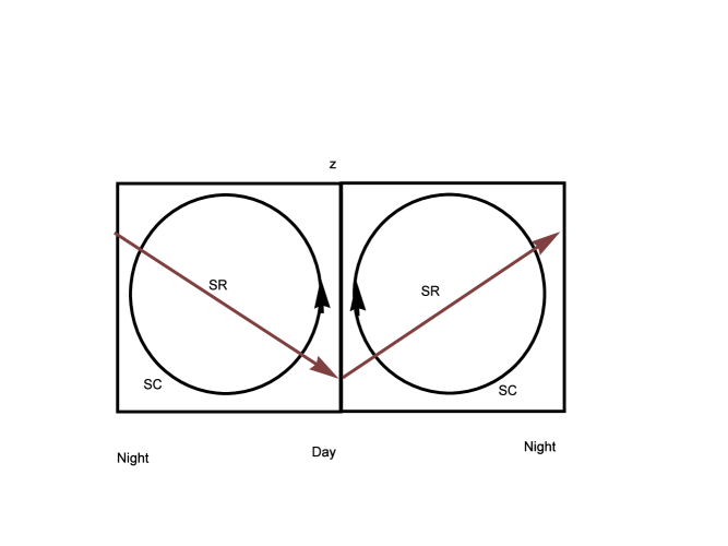
Figure 1: Schematic patterns of the bilaterally symmetric-circulation (SC) and asymmetric super-rotation (SR). The horizontal direction of the plane represents the equator of the Venus, with right and left ends identified with each other. The vertical direction represents the height of the atmosphere. Note the SC respects the bilateral symmetry of the meridian plane passing through the day point and the two poles, while SR violates this symmetry.

There have been many studies to explain SR from various points of view. Schubert and WhiteheadSchubert1969 , and ThompsonThompson1970 have considered a shift of the day-night convective circulations. They considered a possible overall shift of the circulations toward the planet rotational direction that might induce the super-rotation. The idea would be natural, however, this pair of bilaterally symmetric-circulations (SC) cannot smoothly connect to SR dominated flow(Fig.1). This is because the flow speeds at a high and low altitude of the circulations are the same with each other. Therefore SR, that lacks the circulation at the low altitude, is impossible.

In order to overcome this difficulty, we introduce an extra circulation rotating around the planet at low altitude. The superposition of these three circulations can express the SC as well as SR at the same time. The flow of SC respects the bilateral symmetry about the meridian section defined by the day point, North/South poles, and the night point. On the other hand, the flow of SR violates this symmetry. Therefore our task is to find a mechanism of transition from SC to SR, i.e. the violation of the symmetry.

Subsequently, many researchers considered the explicit mechanism of this symmetry breaking searching for concrete driving forces for SR. Fels and LindzenFels1974 considered the thermally excited gravity waves at the cloud top regions. Hou and FarrellHou1987 considered the propagation of the gravity waves upward. GieraschGierasch1975 considered the systematic shift of the meridian circulations. MatsudaMatsuda1980 ; Matsuda1982 extracts several relevant flow modes and considered their non-linear interactions based on GieraschGierasch1975 . All of them considered the explicit symmetry breaking based on the principle: Symmetric mode interactions do not yield asymmetryMatsuda1983 . Therefore the planetary rotation was essential for generating SR.

We recognize, however, the flow of atmosphere is a heat engine system that autonomously works by getting energy mainly from the Sun and dumping the heat toward the interstellar space. The basic architecture of an engine is the linear system composed of a piston and a cylinder. This linear oscillatory motion of the piston is transformed into the rotational motion of a wheel either to the right or left. The bilateral symmetry is spontaneously broken at this stage. Any small trigger or random fluctuation in the joint or initial condition is needed to determine the rotational direction. The power of the rotation is maintained by that of the piston and not by the detailed mechanism of the joint. Moreover, the time scale for the wheel to reach the steady state would not depend on the strength of the trigger but depends on the power generated at the cylinder.

In this paper, we reconsider the basic mechanism how SR is possible. We first estimate the number of zonal bands of flow for each planet in sec.II. We find the Venus and the Titan will possibly have a single zone flow. We next introduce the three-loop model for SC and SR and demonstrate several typical time evolution of flow patterns in section III. In section IV, we find stationary points which correspond to SC and SR with the associated stationary temperature differences. Next, in section V, we clarify the Physics behind our model; spontaneous symmetry breaking and the maximum flow principle. In section VI, we estimate the parameters in our phenomenological model based on several observational data. In section VII, we compare our model with other models so far proposed. In the last section VIII, we close our study summarizing our work and prospects.

II Number of Coriolis-drive zonal bands

The number of atmospheric flow bands rotating around the planet is determined by the meridional circulation and the Coriolis force. The Coriolis force makes the meridional circulation velocity $v$ toward the longitudinal direction of amount $-2\Omega\times v$. Within the time interval $\tau$, the meridional flow travels the distance $l\approx\tau v$, and the Coriolis acceleration $\approx 2\Omega v$ makes the flow deviate toward the longitudinal direction about$\approx\left(1/2\right)2\Omega v\tau^{2}$. If we set this distance as $l$, then we can estimate the distance for the meridional flow turns its direction about $\pi/2$. Thus we have $\tau\approx\Omega^{-1}$ and the characteristic distance for the meridional flow becomes $l\approx v/\Omega$. If we divide the full meridional distance of the planet by this amount, we can roughly estimate the number of segments of the meridional circulation,

$$\#\mathrm{band}=1+\frac{\pi\cdot\left(\mathrm{planetary\,radius}\right)}{v\cdot\left(\mathrm{rotation\,period}\right)}.$$ (1)

This is also the number of (local) super-rotation (SR) bands or jet streams. It is important to notice that the Coriolis force simply shifts the existing flow but never accelerates the flow. Reflecting the fact that the adjacent meridional circulation has the parallel flow interface (i.e. opposite circulation directions), the zonal bands or jet streams have alternating rotational directions. The estimated zonal band numbers according to the Eq.(1) is given in the Table 1.

$\begin{array}[]{|c|c|c|c|c|}\hline\cr\text{Name}&\text{Radius(km)}&\text{Rotation Period(hour)}&\text{Surface Pressure(bars)}&\text{estimated zone number}\\ \hline\cr\text{MERCURY}&2439.5&4222.6&0&1.00672\\ \hline\cr\text{VENUS}&6052.&2802&92&1.03\\ \hline\cr\text{EARTH}&6378.&24&1&4.09\\ \hline\cr\text{MOON}&1737.5&708.7&0&1.02853\\ \hline\cr\text{MARS}&3396.&24.7&0.01&2.59977\\ \hline\cr\text{JUPITER}&71492.&9.9&\text{Unknown*}&85.025\\ \hline\cr\text{SATURN}&60268.&10.7&\text{Unknown*}&66.5374\\ \hline\cr\text{URANUS}&25559.&17.2&\text{Unknown*}&18.2903\\ \hline\cr\text{NEPTUNE}&24764.&16.1&\text{Unknown*}&18.897\\ \hline\cr\text{PLUTO}&1185.&153.3&0&1.08994\\ \hline\cr\text{Titan}&2575.5&382.&1.45&1.07845\\ \hline\cr\end{array}$

Table 1: Table of the planet data NASA2017 and the estimated number of zonal flow bands from Eq.(1). We have taken a representative value for the flow speed as $v=75$meter/sec. Actual numbers of flow bands vary in time and may have substructures especially in big planetsRogers2017 . The estimated band number qualitatively represents the actual number.

According to this table, the zonal band number of Mercury, Venus, Our Moon, Pluto, and Titan are almost one. This fact suggests that these planets (satellites) have a single zonal band flow or the (global) SR for each if they have an atmosphere. Consulting the surface pressure, we expect that Venus and Titan will probably have the (global) SR, and Mercury, Our Moon, and Pluto are excluded.

III Three-loop model for flows

We study the planets/satellites with a single zonal band flow such as Venus and Titan. For this purpose, we introduce the following model composed of three loops of circulating flows (Fig.2). Their velocities are $v_{1}\left(t\right),v_{2}\left(t\right),v_{3}\left(t\right)$, and the temperature difference between the day and night points is $\theta\left(t\right)>0$. These four variables are our basic degrees of freedom in the model. They obey the set of time evolution equations,

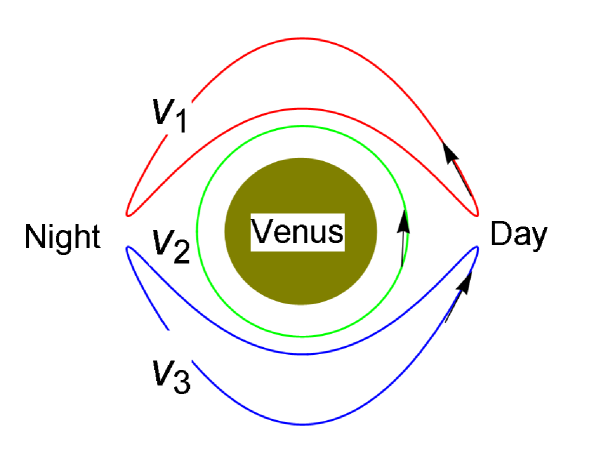
Figure 2: The three loop model for the Venus atmosphere described by Eq.(2). The arrow defines the positive direction for each circulation. The superpositions of these flows represent actual flows at high and low altitude layers. These circulations interact with each other through viscosity. The loop pair 1-2 and 3-2 tend to be parallel, while the pair 1-3 tends to be anti-parallel. The total system has two types of typical flows: +,+,+ (-,-,-), and +,0,- (-,0,+), for the signatures of $v_{1}\left(t\right),v_{2}\left(t\right),v_{3}\left(t\right)$, respectively. The former represents SR and the latter SC.

$$\begin{aligned} \frac{dv_{1}}{dt}\text{$=$- $\nu$}v_{1}+R+av_{1}\theta-\kappa\left(v_{1}\text{-}v_{2}\right)\text{-$\frac{\mu}{2}$ (}v_{1}\text{+}v_{3}\text{), }\\ \frac{dv_{2}}{dt}=\kappa(v_{1}\text{-}v_{2}\text{)+ $\kappa$ (}v_{3}\text{-}v_{2}\text{)}\text{, }\\ \frac{dv_{3}}{dt}\text{$=$- $\nu$}v_{3}+R+av_{3}\theta\text{-$\kappa\left(v_{3}\text{-}v_{2}\right)$}-\frac{\mu}{2}(v_{3}\text{+}v_{1}\text{), }\\ \frac{d\theta}{dt}=h-b(v_{1}^{2}+v_{3}^{2})\theta.\end{aligned}$$ (2)

Our parameters are the triggering force $R$, temperature drive efficiency $a$, the energy transfer efficiency $b$, the incoming heat rate $h$, horizontal viscosity at the lower layer$\kappa$, the vertical viscosity $\mu$, and the viscosity at the higher layer $\nu$. The vertical viscosity $\mu$ promotes the bilaterally symmetric-circulations for the flows $v_{1}$ and $v_{3}$. The horizontal viscosity at the lower layer$\kappa$ is effective for actual flow $(v_{1}\text{-}v_{2})$ and $\text{(}v_{3}\text{-}v_{2}\text{)}$, and makes the coupling between all the three flows $v_{1}$ through $v_{3}$.

All the terms are bilaterally symmetric and do not distinguish east-west directions except the triggering force $R$. In other words, the set of equations, except $R$, is invariant under the mirror transformation: $v_{1}\rightarrow-v_{3},v_{2}\rightarrow-v_{2},v_{3}\rightarrow-v_{1},\theta\rightarrow\theta$. There are two kinds of typical flows described by the above set of equations, one respects the symmetry (SC) and the another violates it (SR). We will see that the latter type of flow SR appears spontaneously and is drove by the heat $h$ even within the symmetric situation $R=0$.

The evolution equations for the flows $v_{i}$ can be written by the following quasi-potential $V$

$$V=\frac{\kappa}{2}\left(\left(v_{1}-v_{2}\right)^{2}+\left(v_{3}-v_{2}\right)^{2}\right)+\frac{\mu}{4}\left(v_{1}+v_{3}\right)^{2}+\frac{1}{2}\left(\nu-a\theta\right)\left(v_{1}^{2}+v_{3}^{2}\right)-R\left(v_{1}+v_{3}\right)$$ (3)

as

$$\frac{dv_{i}}{dt}=-\frac{dV}{dv_{i}},$$ (4)

for $i=1,2,3$. The first two terms in $V$, each proportional to the difference/summation of the velocities, represent the momentum conservation, while the last two terms represent genuine dissipation and the source term.

If we neglect the explicit trigger term $R\rightarrow 0$, the potential is entirely quadratic. Therefore, multiplying $v_{i}$ to the both sides of Eq.(4) and summing over $i=1,2,3$, we obtain

$$\frac{dK}{dt}=-\sum_{i}\frac{dV}{dv_{i}}v_{i}=-2V,$$ (5)

where $K\equiv\left(1/2\right)\sum_{i}\dot{v}_{i}^{2}$ is the strength of the total flow or the kinetic energy. Thus, the quasi-potential $V$ drives the total flow.

We show some results obtained from the numerical calculations of our model. It will become clear that the typical flow modes, SC or SR, are mainly determined by the parameters $\kappa$ and $\mu$. Therefore we first examine the case that the explicit driving is absent $R$=0.

In Fig.3 and Fig.4, we demonstrate that the parameter $\kappa$ drives SR while $\mu$ drives SC. The SR on Venus and Titan thus correspond to the case $\kappa>\mu$.

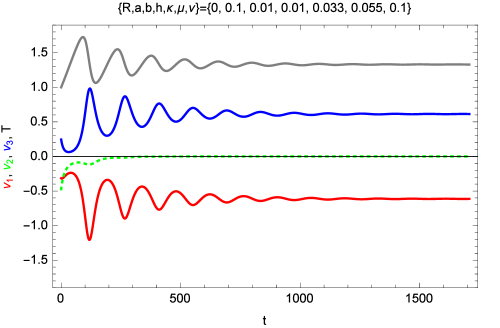
Figure 3: Time evolution of the three flows $v_{1}$(red), $v_{2}$(green dotted), $v_{3}$(blue), and the temperature difference $\theta$(gray) in the SC mode for the case $\kappa<\mu$. The explicit triggering force is absent $R=0$.

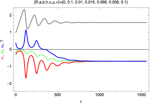
Figure 4: The same as Fig. 3, but in the SR mode for the case $\kappa>\mu$. The explicit triggering force is absent $R=0$.

If both the parameters are almost equal $\kappa\approx\mu$, then the two modes SC and SR compete with each other to yield strong fluctuations during the transition (Fig.5). In this case (Fig.5), SC finally dominates since $\kappa<\mu$.

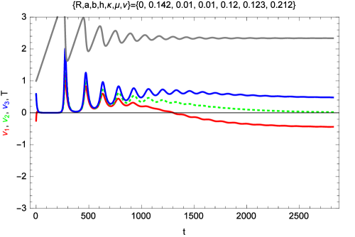
Figure 5: The same as Fig. 3 but shows the transition from SR to SC for the case $\kappa\approx\mu$ with $\mu$ slightly larger than $\kappa$. The explicit triggering force is absent $R=0$.

In general, the case $\kappa\approx\mu$ is delicate as expressed in Fig.6. The fate of the flow is quite dependent on the initial conditions and any small fluctuations in the actual case. In other regions, either SR or SC is realized independently from the initial conditions.

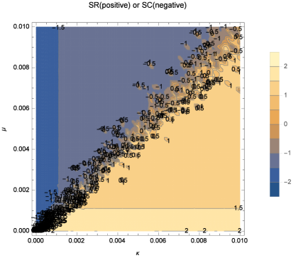
Figure 6: The final values $v_{1}v_{3}$ at the end of various runs for different parameters $\kappa$ and $\mu$ with many random initial conditions ($-1<v_{1},v_{2},v_{3}<1$, and $\theta=1$). The other parameters are fixed to be $R=0,a=0.2,b=0.01,\nu=0.02$, and each run starts at the time $0$ to $500$. A positive value of $v_{1}v_{3}$ means the flow 1-2 have the same direction while a negative value of $v_{1}v_{3}$ means they have the opposite direction. The explicit triggering force is absent $R=0$.

If the explicit triggering force $R$ exists, the situation is quite different (Fig.7). SR flow is directly triggered almost independently from the values of $\mu$ and $\nu$. The the local SR on the Earth and Jupiter will correspond to this case $R>0$.

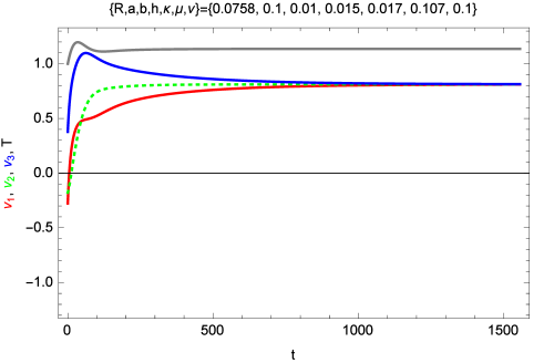
Figure 7: The same as Fig. 3, but now we have the explicit triggering force $R$ which drives SR. In this case, the effect of the force $R$ dominates even if $\kappa<\mu$.

IV Parameter space and the stationary states

We clarify the characteristic behaviors of the flow evolution demonstrated in the previous section. The relevant parameters of our model Eq.(2) are…$\kappa,\mu,\nu$ for the interactions between flows, and $a,b$ for flow-heat coupling, and $h,R$ for the driving force. We will find the possible fixed stationary points of Eq.(2) for the variables $v_{1},\;v_{2},\;v_{3},\;\theta$. Setting the left-hand sides $0$ in this set of equations and solving for these variables, the general fixed points are found to be, in the form of $\{v_{1},\;v_{2},\;v_{3},\;\theta\}$,

$$\begin{array}[]{cccc}\{v_{-}^{SR},&v_{-}^{SR},&v_{-}^{SR},&\theta_{+}^{SR}\},\\ \{v_{+}^{SR},&v_{+}^{SR},&v_{+}^{SR},&\theta_{-}^{SR}\},\\ \{v_{-}^{SC},&-\frac{R}{\kappa-\mu},&v_{+}^{SC},&\frac{\kappa+\nu}{a}\},\\ \{v_{+}^{SC},&-\frac{R}{\kappa-\mu},&v_{-}^{SC},&\frac{\kappa+\nu}{a}\},\end{array}$$ (6)

where

$$v_{\pm}^{SR} \equiv\frac{R\pm\sqrt{2\left(a/b\right)h\left(\mu+\nu\right)+R^{2}}}{2\left(\mu+\nu\right)},\;v_{\pm}^{SC}\equiv\frac{\pm\frac{\sqrt{\left(a/b\right)h\left(\kappa-\mu\right)^{2}-2R^{2}(\kappa+\nu)}}{\sqrt{2}\sqrt{\kappa+\nu}}-R}{\left(\kappa-\mu\right)},$$ (7)

$$\theta_{\pm}^{SR} \equiv\frac{\pm\sqrt{b}R\sqrt{2ah\left(\mu+\nu\right)+bR^{2}}+ah\left(\mu+\nu\right)+bR^{2}}{a^{2}h}.$$ (8)

These four fixed points are too complicated. Therefore we reduce the expression assuming the relevant case $R\rightarrow 0$ where the evolution equation Eq.(2) is fully symmetric. Then Eq.(6) reduces to the form

$$\begin{array}[]{cccc}\{-\sqrt{\frac{ah}{2b\left(\mu+\nu\right)}},&-\sqrt{\frac{ah}{2b\left(\mu+\nu\right)}},&-\sqrt{\frac{ah}{2b\left(\mu+\nu\right)}},&\frac{\mu+\nu}{a}\},\\ \{\sqrt{\frac{ah}{2b\left(\mu+\nu\right)}},&\sqrt{\frac{ah}{2b\left(\mu+\nu\right)}},&\sqrt{\frac{ah}{2b\left(\mu+\nu\right)}},&\frac{\mu+\nu}{a}\},\\ \{-\sqrt{\frac{ah}{2b\left(\nu+\kappa\right)}},&0,&\sqrt{\frac{ah}{2b\left(\nu+\kappa\right)}},&\frac{\kappa+\nu}{a}\},\\ \{\sqrt{\frac{ah}{2b\left(\nu+\kappa\right)}},&0,&-\sqrt{\frac{ah}{2b\left(\nu+\kappa\right)}},&\frac{\kappa+\nu}{a}\}.\end{array}$$ (9)

These four fixed points represent, in order, left and right rotating SR, and left and right circulating SC (Fig.2). The choice of either the left or the right rotating SR violates the bilateral symmetry of the Eq.(2), while SC respects the symmetry. We find again that the distinction between SR and SC is summarized in the parameters $\mu,\nu$ as apparent in the above expressions. We also find the flow speed squared is always inversely proportional to the temperature $v^{2}=\left(h/2b\right)/\theta$. We further find that the triggering force term $R$ turns out to kill the SC mode for $R>R_{c}$ where

$$R_{c}=\left(\frac{ah\left(\kappa-\mu\right)^{2}}{2b\left(\kappa+\nu\right)}\right)^{1/2}$$ (10)

since $v_{\pm}^{SC}$ becomes complex then.

If the entire flow were due to the triggering force $R$, then the symmetry is explicitly broken. Putting $h\rightarrow 0$, we have the stationary points, for $\{v_{1},\;v_{2},\;v_{3},\;\theta\}$, as

$$\begin{array}[]{cccc}\{0,&0,&0,&*\},\\ \{\frac{R}{\left(\mu+\nu\right)},&\frac{R}{\left(\mu+\nu\right)},&\frac{R}{\left(\mu+\nu\right)},&*\},\\ \{v_{-}^{SC},&\frac{R}{\mu-\kappa},&v_{+}^{SC},&*\},\\ \{v_{+}^{SC},&\frac{R}{\mu-\kappa},&v_{-}^{SC},&*\},\end{array}$$ (11)

where the velocity of the symmetric flow SC always becomes complex

$$v_{\pm}^{SC}\equiv\frac{\left(1\pm i\right)}{\kappa-\mu}R$$ (12)

and $"*"$ means being indeterminate. Thus the mode SC is fully killed and only the SR survives whose speed is simply proportional to the force $R$.

We now study the stability of the fixed points obtained above. The right-hand side of Eq.(2) linearized, in the coordinate $\left(\begin{array}[]{cccc}v_{1}&v_{2}&v_{3}&\theta\end{array}\right)$, becomes

$$\left(\begin{array}[]{cccc}\begin{array}[]{c}a\theta-\kappa-\frac{\mu}{2}-\nu\\ \kappa\\ -\frac{\mu}{2}\\ av_{1}\end{array}&\begin{array}[]{c}\kappa\\ -2\kappa\\ \kappa\\ 0\end{array}&\begin{array}[]{c}-\frac{\mu}{2}\\ \kappa\\ a\theta-\kappa-\frac{\mu}{2}-\nu\\ av_{3}\end{array}&\begin{array}[]{c}-2b\theta v_{1}\\ 0\\ -2b\theta v_{3}\\ -b\left(v_{1}^{2}+v_{3}^{2}\right)\end{array}\end{array}\right).$$ (13)

The eigenvalues of this matrix evaluated by the solutions Eqs.(6,9) give the instability of the individual solutions. If we set $R=0$ and using Eq.(9), we get the following instability by numerical calculations. For the case $\mu>\kappa$, the first two lines of solutions of Eq.(9) (SR) give 1 positive and 3 negative eigenvalues, with some imaginary part in the latter. This means SR mode is unstable with damping oscillatory behavior. On the other hand the last two lines of solutions of Eq.(9) (SC) give 4 negative eigenvalues, with some imaginary part in there. This means SC mode is stable. In this case, the velocity of SC mode is faster than SR mode and the temperature difference $\theta$ for SC is smaller than that for SR as is seen in Eq.(9).

For the opposite case $\mu<\kappa$, SR gives 4 negative eigenvalues while SC gives 1 positive and 3 negative eigenvalues. This means that SR mode is stable. In this case, SR mode is faster and $\theta$ is smaller than those of SC mode.

Summarizing the (in)stability, we conclude that the flow always chooses the faster mode, or the flow always choose the lower temperature. This also means that the flow automatically chooses the most efficient mode of heat transfer.

V Physics behind the generation of SR mode

We have introduced a simplest model Eq.(2) for describing the SR excluding any secondary effects as much as possible. This is because we want to clarify the physics of SR before the elaborate study on the individual detail. Therefore in this section, we study basic physics behind our model.

We first emphasize that the model Eq.(2) is minimal and simplest in the following sense.

1. (three loops) The model is composed of three flow loops of velocities $v_{1},v_{2},v_{3}$. If it were two-loop, the two kinds of flow modes SR and NR cannot be described in the same model. This is because the speeds of the upper and lower region have the same amount all the timeThompson1970 . This is not the property of SR.

2. (dynamical temperature) The temperature difference $\theta(t)$ appears as a dynamical variable. If it were a constant parameter, then the model does not show the spontaneous symmetry breaking. Even the multiply coupled Lorenz model Lorenz1963 is not enough for our purpose because the external temperature difference is fixed from the beginning. The flow that carries heat must have feedback effect for the reduction of the source temperature.

3. (non-linearity) Our model has nonlinear terms that come from the velocity-temperature couplings $av_{1}\theta,av_{3}\theta,$and $b(v_{1}^{2}+v_{3}^{2})\theta$. These couplings have been chosen so that it does not destroy the bilateral symmetry of the system. The ultimate origin of them would be the advection term. However, there will appear many nonlinear terms in actual situations, such as the velocity dependent convection and turbulent fluctuations. Provided they respect the symmetry, these nonlinear terms will not drastically change our model as we have already checked some of them. We believe our nonlinear terms are minimal.

4. (extra loop under the symmetric loops). We set an extra rotating loop $v_{2}$ under the symmetric-circulation loops $v_{1},v_{3}$. If this extra loop were set over the symmetric loops, then $v_{1},v_{3}$ eventually reduce for the horizontal friction near the planet surface. This further reduces $v_{2}$ as well for the loop couplings. Setting the extra loop under $v_{1},v_{3}$ helps the reduction of the overall speed under circulations, $v_{1}-v_{2},v_{3}-v_{2}$, and leaving high-speed outer rotation $v_{1},v_{3}$.

There are two basic physics in our model; spontaneous symmetry breaking (SSB) and the possible maximum flow principle (MFP).

Spontaneous symmetry breaking (SSB) is very general phenomena we encounter everywhere. Our model Eq(2) respects the bilateral symmetry and does not distinguish east-west directions ($v_{1}\rightarrow-v_{3},v_{2}\rightarrow-v_{2},v_{3}\rightarrow-v_{1},\theta\rightarrow\theta$), except the triggering force $R$ which we neglect for the moment. However, the symmetry can be violated at the solution level. This situation is schematically shown in Fig.8. The horizontal axis represents any order parameter, the indicator of the bilateral symmetry violation, say $v_{1}+v_{3}$. The vertical axis represents any indicator of the stability, the lower the position the more stable, say the temperature difference $\theta$. The flow SC respects the symmetry while SR violates this symmetry. This violation mode SR can appear spontaneously whenever this mode is more stable than the others.

The planetary atmosphere is a heat engine. The heat injection from the sun yields work from the system and the remaining heat flows out into space. Any tiny trigger or any random initial condition, as well as the explicit trigger $R$, can decide the initial rotational direction whichever. The non-linearity of the system enhances the rotation to this direction. This mechanism is the same as the ordinary engine with a linear cylinder and piston. The linear periodic motion of the piston and the rod gradually enhance and establish the rotational motion of either direction.

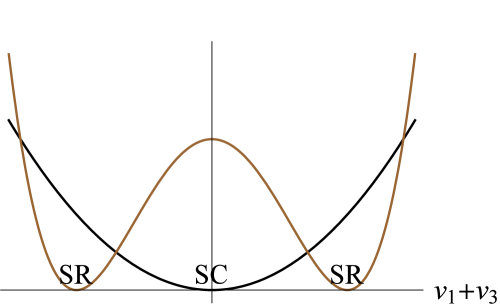
Figure 8: Schematic diagram of the spontaneous breaking of the bilateral symmetry. The horizontal axis represents any order parameter, the indicator of the bilateral symmetry violation, say the combination of the variables $v_{1}+v_{3}$. The vertical axis represents any indicator of the stability, the lower the position the more stable, say the temperature difference $\theta$. The flow mode SC respects the symmetry while SR doesn’t. The flow mode SR appears spontaneously without resorting to the explicit symmetry violating force such as $R$.

The maximum flow principle (MFP) is another essence of our model. There are multiple modes for the heat propagation in general heat system. Depending on the boundary or initial conditions, the system often chooses the most efficient mode for heat transfer autonomously. In our case, we have typically SC and SR modes. SC respects the bilateral symmetry and SR violates it. As we have seen at the end of the last section, when the parameters satisfy $\kappa<\mu$, SC mode is autonomously chosen. This SC flows faster and therefore the temperature difference reduces, thus is more efficient than SR mode. On the other hand, when $\kappa>\mu$, more efficient flow SR is chosen.

This tendency of MFP seems to be common in various cases. For example for water boiling, the heat transfer modes changes, in the order of increasing temperature difference, conduction, convection, nucleate boiling, and passing through the phase of transition boiling, finally reaches to the film boilingNukiyama1934 . The efficiency of the heat transfer actually increases in this order. MFP will be one of the common rules that govern the non-equilibrium phenomena of fluid. However, the theoretical formulation of this kind of variational principle for thermo-fluid dynamics far from equilibrium seems not to be established yetOnsager1953 .

Finally, I should mention that the above SSB and MFP are closely related to each other. Ordinary SSB requires an effective potential that determines the stability, while in our case, we do not have such potential. The best indicator of stability would be the flow efficiency or the temperature $\theta$. In this sense, our SSB is special and is supported by the MFP.

VI Observational aspects

We now try to constrain our model parameters from available observational data. The vertical temperature profile of Venus atmosphere is observed Seiff1983 and the fluctuations are not small especially in the higher layers: at the height $65km$, the temperature is $220-250K$ and at $90km$ and higher, $160-190K$. If we can interpret the fluctuation as the day and night temperature difference $\theta$ at the SR zone in the mesosphere, it becomes $\theta_{M}=30K$ at most. Another possibility would be that the day and night temperature difference $\theta$ comes from the difference in heights for the SR. If the SR layer were higher at the night region (colder) and were lower at the day region (hotter), then we have $\theta=60K$ at most. Suppose we take $\theta_{M}=30K$ below. On the other hand in the much higher thermosphere, higher than 120km, $\theta_{T}=150K$ where the flow may be SCBertaux2007 . Therefore we have

$$\frac{\theta_{T}}{\theta_{M}}\approx\frac{150K}{30K}=5.$$ (14)

According to Eq.(9) at the stationary points, we have the relationship between the wind speed and the temperature,

$$v^{2}=\frac{ah}{2b\theta}$$ (15)

irrespective of SR or SC. Then from the temperature ratio, we can estimate the wind speed ratio, assuming $a,b$ are respectively the same at thermosphere and mesosphere,

$$\left(\frac{v_{T}}{v_{M}}\right)^{2}=\frac{\theta_{M}}{\theta_{T}}\frac{h_{T}}{h_{M}}=\frac{1}{5}\frac{h_{T}}{h_{M}}.$$ (16)

Since we naturally expect, from the existence of the heavy cloud of $H_{2}SO_{4}$, that $h_{M}>h_{T}$, we estimate $v_{T}$ is much smaller than $v_{M}$.

Observation shows that the flow is SR in the mesosphere, and therefore we expect $\kappa>\mu$ there. On the other hand at the higher thermosphere, the horizontal viscosity $\kappa$ would be far smaller. Therefore the opposite situation $\kappa<\mu$ would be probable there. Then the flow would be SC. At the interface zone, $\kappa\approx\mu$ and the frustration between SR and SC would take place. Therefore flows there would have strong fluctuation as in Fig.6.

We now estimate the parameters of SR zone in the mesosphere of Venus. The main ingredient there is the sulfuric acid $H_{2}SO_{4}$ which has the specific heat $c=1.4$(J/g K). The mass density of the sulfuric acid in the mesosphere is $\rho=4.4\times 10^{2}g/m^{3}$, and the solar energy input is $W=150Watt/m^{2}$. The specific height of this zone is $H=3.0\times 10^{4}m$. Thus we have

$$h=\frac{d\theta}{dE}\frac{dE}{dt}=\text{$\frac{W}{c\rho H}=8.1\times 10^{-6}\frac{K}{\sec}$}.$$ (17)

Using this value and observed wind velocity $v=100m/\sec$, we have

$$b=\frac{h}{2\theta v^{2}}=1.3\times 10^{-11}\frac{\sec}{m^{2}}.$$ (18)

The time scale of the temperature difference $\theta$ therefore becomes

$$\tau_{\theta}=\frac{1}{bv^{2}}=\frac{2\theta}{h}=7.4\times 10^{6}\sec.$$ (19)

The similar time scale for the wind velocity can be roughly estimated to be

$$\tau_{\nu}=\frac{1}{\nu}=4.7\times 10^{8}\sec$$ (20)

from the observations Khatuntsev2013 ; Kouyama2013 claiming that the SR velocity had changed $40m/\sec$ within 6 years. If we suppose the parameters $\mu$ and $\nu$ have almost the same order,

$$a=\frac{\mu+\nu}{\theta}\approx\frac{\nu}{\theta}=7.0\times 10^{-11}K^{-1}\sec^{-1}.$$ (21)

On the other hand, the Saturn’s satellite Titan is a candidate of the global SR according to the argument of the section II. However, the study for the Titan SR seems to be complicated by relatively large deviation of the spin axes $26.7^{o}$. Therefore we skip the case of Titan SR in this paper.

VII Comparison with other models

We compare our model with the others so far proposed to explain SR mainly of Venus.

We have set up three loop model to describe SR and SC. On the other hand, Schubert and WhiteheadSchubert1969 , and ThompsonThompson1970 proposed a model of two loops, representing the day-night convective circulations, that are shifted by the planetary rotation. The time lag, in their case, due to the propagation of the temperature difference upward, is expected to shift the day-night convective circulation. Thus the planetary rotation is essential to maintain SR. However, a simple shift of SC does not fully describe SR whose flow covers the entire planet surface. We believe a set of three loops is indispensable to describe SR as well as SC.

We have emphasized the spontaneous generation of SR in which we do not need an explicit violation of bilateral symmetry of west-east mirror reflection. Therefore the planetary rotation is not essential to yield and maintain SR in our model. On the other hand, most of the other models explicitly breaks the symmetry for example by the thermally excited gravity waves at the cloud top regions (Fels and LindzenFels1974 ), or by the propagation of the gravity waves upward (Hou and FarrellHou1987 ), or by the systematic shift of the meridian circulations (GieraschGierasch1975 and extended by MatsudaMatsuda1980 ; Matsuda1982 ). All of them considered the explicit symmetry breaking based on the principle: Symmetric mode interactions do not yield asymmetryMatsuda1983 . Therefore the planetary rotation is ultimately essential for generating SR in their cases, quite contrary to our model. However, the planetary rotation or the Coriolis force may trigger the symmetry breaking especially for the cases of Venus and Titan.

We have extracted the essential circulation modes and try to analyze them in the analytic method. This point is parallel to Matsuda Matsuda1980 , YamamotoYamamoto2013 , Kashimura and Yoden Kashimura2015 . They developed simplified model extending the mechanism of GielashGierasch1975 . Their relevant parameters roughly correspond to ours. For example, the thermal Rossby number $R_{T}=gH\Delta_{H}a^{-2}\Omega^{-2}$ would correspond to our parameter $h$, the vertical Ekman number $E_{V}=\nu_{V}a^{-2}\Omega^{-1}$to $\mu$, the horizontal Ekman number $E_{H}=\nu_{H}a^{-2}\Omega^{-1}$ to $\nu$, where $H$ is the height of the top boundary, $\Delta_{H}$ is the fractional change in potential temperature from the equator to the pole, $a$ is the planetary radius, $\Omega$ is the angular velocity of the planetary rotation, $g$ is the gravitational acceleration, $\nu_{H}$ and $\nu_{V}$ are respectively the horizontal and vertical diffusion coefficients. However, the correspondence is not complete for example, we do not normalize the parameters by $\Omega$.

We have derived the expression for SR for Venus as Eq.9, and the SR velocity is given by

$$v_{SR}=\sqrt{\frac{ah}{2b\left(\mu+\nu\right)}},$$ (22)

which is independent of the explicit driving force $R$ or $\Omega$; SR appears spontaneously. Therefore SR would be observed even for the static planet without rotation $\Omega=0$, or more precisely the planet with fixed day-night hemispheres.

On the other hand, GieraschGierasch1975 obtained the SR velocity as

$$U=\Omega a\exp\left(D^{2}HW/\nu_{v}\right),$$ (23)

where $\Omega$ is the angular velocity, $a$ is the Venus radius, $D$ is the mean scale height, $H$ is depth in scale heights, $W$ is the inverse of the meridional overturning time, and $\nu_{v}$ is the vertical eddy diffusivity. It is apparently proportional to the angular velocity and $U$ vanishes for no planetary rotation; SR is generated by the explicit symmetry breaking force. However, the force $R$ would trigger the SR of Venus and Titan, and becomes essential to drive the local SR for the other planets such as Earth and Jupiter.

VIII Conclusions and prospects

We constructed a three loop model which describes super-rotation (SR) as well as symmetric-circulation (SC) of the planetary atmosphere. The set of equations describing the time evolution of the circulation velocities $v_{1}\left(t\right),v_{2}\left(t\right),v_{3}\left(t\right)$ and the temperature difference $\theta\left(t\right)$ respects the bilateral mirror symmetry about the meridian section defined by the day/night points and poles, except terms of $R$. We demonstrated that the asymmetric flow pattern SR is spontaneously generated in our model as well as the symmetric SC. Our model is minimal which has this property. These SR and SC modes are generally in frustration with each other and the faster flow, or much efficient flow, is spontaneously realized depending on the given parameters. In general, the planetary atmosphere is a thermal engine and the zonal rotation flow is naturally generated irrespective of globally or locally. We could constrain the parameters of our phenomenological model. Many sophisticated mechanisms so far studied, such as the mechanism based on the night-day circulation, on the meridian circulation, on the thermally excited gravity waves, will be important to trigger SR and to determine the direction of SR. However, the SR is quite general and can be spontaneously generated irrespective of the detail of trigger.

We did not consider the intrinsic fluctuations of the flow and therefore our model is deterministic. Actually, the atmospheric circulation of a planet is a huge system including many degrees of freedom. Therefore the random fluctuations must exist on top of the dynamics of relevant variables. This fluctuation effect would be easily realized by introducing some appropriate random force term in our model. This may cause an intermittent transition between SR and SC modes in some situations. Large fluctuations would be crucial in particular for describing the local SR of the Earth and the Jupiter.

We did not consider the complete physical derivation of our model but it was simply proposed phenomenologically. A natural method would be to extend the Lorenz model to include higher harmonic modes. It may also work if we couple three Lorenz models. In either case, we need to include full feedback to the temperature which was absent in the original Lorenz model, in which only small fluctuations allowed around a fixed linear temperature gradient. Furthermore, we need to describe the origin of the non-linearity of the flow which was essential for describing the spontaneous SR generation in the present paper.

We would like to report soon our further study on SR developing the improved model reflecting the above points.

- (1) Bengtsson, L., Roger-M. Bonnet, R. M., Grinspoon, D., Koumoutsaris, S., Lebonnois, S., & Titov, D. (2013). Towards Understanding the Climate of Venus. Springer.
- (2) Schubert, G. and J. A. Whitehead, 1969: Moving ame experiment with liquid mer- cury: Possible implications for Venus atmosphere, Science, 163 (3862), 71-72.
- (3) Thompson, R., 1970: Venus’s general circulation is a merry-go-round, J. Atmos. Sci., 27 (8), 1107-1116.
- (4) Fels, S. B. and R. Lindzen, 1974: The interaction of thermally excited gravity waves with mean ows, Geophys. Fluid Dyn., 6 (2), 149-191.
- (5) Hou, A. Y. and B. F. Farrell, 1987: Superrotation induced by critical-level absorption of gravity-waves on venus|an assessment, J. Atmos. Sci., 44 (7), 1049-1061.
- (6) Gierasch, P. J., 1975: Meridional circulation and maintenance of the Venus atmo- spheric rotation, J. Atmos. Sci., 32 (6), 1038-1044.
- (7) Matsuda, Y., 1980: Dynamics of the four-day circulation in the Venus atmosphere, J. Meteor. Soc. Japan, 58 (6), 443-470.
- (8) Matsuda, Y., 1982: A further study of dynamics of the four-day circulation in the Venus atmosphere, J. Meteor. Soc. Japan, 60 (1), 245-254.
- (9) Matsuda, Y., 1983: Classification of Critical Points and Symmetry-Breaking in Fluid Phenomena and its Application to Dynamic Meteorology. J. Meteor. Soc. Japan, 61, 771-788.
- (10) Planetary Fact Sheet - the NSSDCA! - NASA, https://nssdc.gsfc.nasa.gov/planetary/factsheet/
- (11) John H. Rogers, Journal of the British Astronomical Association (in press) https://arxiv.org/abs/1707.03343
- (12) Lorenz, Edward Norton (1963). ”Deterministic nonperiodic flow”. Journal of the Atmospheric Sciences. 20 (2): 130–141.
- (13) Onsager, L. and Machlup S. 1953. Fluctuations and Irreversible Processes. Phys. Rev. 91: 1505-1512.
- (14) A. Seiff, Thermal structure of the atmosphere of Venus, in Venus, (A83-37401 17-31), ed. by D.M. Hunten, L. Colin, TM. Donalme, V.I. Moroz., pp. 2 LS-279 (Tucson, AZ, University of Arizona Press, I 983).
- (15) Bertaux, Jean-Loup; Vandaele, Ann-Carine; Korablev, Oleg; Villard, E.; Fedorova, A.; Fussen, D.; Quémerais, E.; Belyaev, D.; et al. (2007). ”A warm layer in Venus’ cryosphere and high-altitude measurements of HF, HCl, H2O and HDO”. Nature. 450 (7170): 646–649.
- (16) Yamamoto, H. and S. Yoden, 2013: Theoretical Estimation of the Superrotation Strength in an Idealized Quasi-Axisymmetric Model of Planetary Atmospheres. J. Meteor. Soc. Japan, 91(2), 119–141.
- (17) H. Kashimura and S. Yoden, Journal of the Meteorological Society of Japan 93 309 2015.
- (18) I.V. Khatuntsev et.al., Icarus 226 (2013) 140–158.
- (19) T. Kouyama et al.,JOURNAL OF GEOPHYSICAL RESEARCH: PLANETS, VOL. 118, 37–46 2013.
- (20) Nukiyama, S., 1934, “The Maximum and Minimum Values of Heat Q Transmitted From Metal to Boiling Water Under Atmospheric Pressure,” Journal of Japanese Society of Mechanical Engineering, Vol. 37, pp. 367-374 (1934) (translated in International Journal of Heat and Mass Transfer, Vol. 9, pp. 1419-1433 (1966)). Nukiyama, S., 1934, “The Maximum and Minimum Values of Heat Q Transmitted From Metal to Boiling Water Under Atmospheric Pressure,” Journal of Japanese Society of Mechanical Engineering, Vol. 37, pp. 367-374 (1934) (translated in International Journal of Heat and Mass Transfer, Vol. 9, pp. 1419-1433 (1966)).