Quasiparticle entropy in superconductor/normal metal/superconductor proximity junctions in the diffusive limit

Abstract

We discuss the quasiparticle entropy and heat capacity of a dirty superconductor-normal metal-superconductor junction. In the case of short junctions, the inverse proximity effect extending in the superconducting banks plays a crucial role in determining the thermodynamic quantities. In this case, commonly used approximations can violate thermodynamic relations between supercurrent and quasiparticle entropy. We provide analytical and numerical results as a function of different geometrical parameters. Quantitative estimates for the heat capacity can be relevant for the design of caloritronic devices or radiation sensor applications.

I Introduction

Recently a growing interest has been put on the investigation of thermodynamic properties of nanosystems, where coherent effects can be both of fundamental interest and useful for applications. Esposito et al. (2009); Campisi et al. (2011); Giazotto et al. (2006); Carrega et al. (2016); Fornieri and Giazotto (2016) In particular, superconductor junction systems have attracted interest, as they exhibit phase-dependent thermal transport enabling coherent caloritronic devices, Giazotto et al. (2006); Giazotto and Martínez-Pérez (2012a); Strambini et al. (2014); Giazotto and Martínez-Pérez (2012b); Martínez-Pérez and Giazotto (2013); Fornieri et al. (2016); Paolucci et al. (2017) and have properties useful for cooling systems in solid-state devices Muhonen et al. (2012); Solinas et al. (2016); Nguyen et al. (2016); Courtois et al. (2016). Conversely, they enable conversion between thermal currents and electric signals, leading to applications in electronic thermometry Saira et al. (2016); Giazotto et al. (2006); Feshchenko et al. (2015) and bolometric sensors and single-photon detectors Wei et al. (2008); Govenius et al. (2016a); Semenov et al. (2002); Engel et al. (2015); Voutilainen et al. (2010); Giazotto et al. (2008); Govenius et al. (2014, 2016b); Karasik et al. (2012). In such applications, detailed understanding of the thermodynamic aspects of hybrid superconducting–normal metal structures is crucial, in particular, the interplay between the energy and entropy related to quasiparticles and supercurrents.

The entropy $S$ of noninteracting quasiparticles at equilibrium is generally determined by their density of states (DOS). In the superconducting state, it is modified by the appearance of an energy gap in the spectrum. In extended Josephson junctions such as superconductor–normal metal–superconductor (SNS) structures, the modification of the DOS depends both on the formation of Andreev bound states inside the junction and the inverse proximity effect in the superconducting banks, both being modulated by the phase difference $\varphi$ between the superconducting order parameters. Likharev (1979); Pannetier and Courtois (2000) Reflecting the fact that the Andreev bound states carry the supercurrent $I$ across the junction, a thermodynamic Maxwell relation

$$\frac{\mathrm{d}{S}\,}{\mathrm{d}\varphi\,}=-\frac{\hbar}{2e}\frac{\mathrm{d}I\,}{\mathrm{d}T\,}=-\frac{\mathrm{d}^{2}F\,}{\mathrm{d}T\,\mathrm{d}\varphi\,}$$ (1)

connects the entropy and the supercurrent to the temperature $T$ and phase derivative of the free energy $F$. The entropy in superconductors can be expressed in terms of the DOS Bardeen et al. (1957) or in terms of Green functions Gor’kov (1959); Eilenberger (1968). Moreover, the phase-dependent part of ${S}$ can be obtained from the current-phase relation $I(T,\varphi)$, Likharev (1979); Golubov et al. (2004), by applying Eq. (1), a contribution important in short junctions Beenakker and v. Houten (1991a, b, a). The different expressions are mathematically equivalent (see e.g. Refs. Kosztin et al., 1998; Kos and Stone, 1999). Such equivalences however can be broken by approximations: in particular, the “rigid boundary condition” approximation Likharev (1979); Golubov et al. (2004), in which the inverse proximity effect in the superconductors is neglected, invalidates DOS-based expressions for entropy. Although such approximations are appropriate for many purposes, they can give wrong results for thermodynamic quantities when boundary effects matter.

Heat capacity Fulde and Moormann (1967); Zaitlin (1982); Kobes and Whitehead (1988) and free energy boundary contributions Hu (1972); Eilenberger and Jacobs (1975); Blackburn et al. (1975); Kos and Stone (1999) in NS systems were considered in several previous works; also experimentally, Lechevet et al. (1972); Manuel and Veyssié (1976) close to the critical temperature $T_{c}$. The inverse proximity effect in the superconducting banks of diffusive NS structures is also well studied. Kupriyanov and Lukichev (1982); Likharev (1979); Blackburn et al. (1975); Golubov et al. (2004) The entropy and heat capacity in diffusive SNS junctions were discussed in Refs. Rabani et al., 2008, 2009, but neglecting the inverse proximity effect, which limits the validity of the results to long junctions only.

In this work, we discuss the proximity effect contributions to the entropy and heat capacity in SNS structures of varying size. We also point out reasons for the discrepancies that appear with the rigid boundary condition approximation in the quasiclassical formalism. We provide analytical results for limiting cases, and discuss the cross-over regions numerically.

The paper is organized as follows. In Sec. II we introduce the theoretical formalism, based on the Usadel equations, and all basic definitions. In Sec. III we discuss the origin of inconsistencies in the rigid boundary condition approximation. In Sec. IV we present quantitative results for the entropy inside the inverse proximity region and the total entropy. We also show results for the heat capacity in Sec. V and the effect of inverse proximity contributions on this quantity. Sec.VI concludes with discussion.

II Model and basic definitions

Here we consider a Josephson junction as schematically depicted in Fig.1(a), where two superconducting banks (S) are in clean electric contact with a normal (N) diffusive wire of length $L_{N}$. The S and N parts are characterized by cross sections $A_{S,N}$ and electrical conductivities $\sigma_{S,N}$, respectively. Microscopically, the two diffusive regions are characterized by the diffusion coefficients $D_{S,N}$ and density of states (DOS) per spin $\mathcal{N}_{0,S}$ and $\mathcal{N}_{0,N}$ at Fermi level. These quantities are related to conductivities via $\sigma_{j}=2e^{2}D_{j}\mathcal{N}_{0,j}$, where, the factor 2 takes into account spin degeneracy.

The presence of superconducting leads induces superconducting correlations in the electrons in the normal metal. The correlations at energy $E$ are associated with a characteristic coherence length $\xi_{E}$, which in general may differ from the superconducting coherence length $\xi_{N/S}\equiv\sqrt{\hbar{}D_{N/S}/|\Delta|}$. The superconductors have order parameter $\Delta$, with phase difference $\varphi$ across the junction. We also assume that the superconductor material has critical temperature $T_{c}$ in bulk.

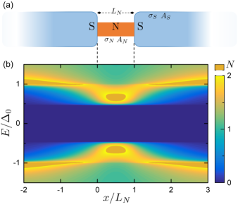
Figure 1: (a) Schematic of a SNS junction consisting of two superconducting (S) leads in clean electric contact with a normal (N) diffusive nanowire of length $L_{N}$. The S and N parts have cross sections $A_{S,N}$ and conductivity $\sigma_{S,N}$. (b) Normalized density of states (DOS) $N(E,x)$ for $\sigma_{S}A_{S}/\sigma_{N}A_{N}=1$, $L_{N}/\xi_{N}=1$ and phase difference $\varphi=0$.

The entropy density ${\cal S}$, and thus the total entropy $S(T,\varphi)=\int{}dx{\cal S}(x,T,\varphi)$, can be written in terms of the quasiparticle spectrum:

$${\cal S}(x,T,\varphi)=\\ =-4{\cal N}_{0}\int_{-\infty}^{\infty}\mathrm{d}E\,N(E,x,\varphi)f(E,T)\ln{f(E,T)}\,,$$ (2)

where $N(E,x,\varphi)$ is the (reduced) local density of states and $f(E,T)=1/(e^{E/T}+1)$ the Fermi distribution function. The normal-state result without proximity effect is found by setting $N(E,x,\varphi)=1$ in the above expression, giving $\mathcal{S}_{n}(T)=2\pi^{3}{\cal N}_{0}T/3$. The entropy density ${\cal S}(x,T,\varphi)$ can also be written as:

$${\cal S}(x,T,\varphi)={\cal S}_{n}(x,T)-\frac{\mathrm{d}\mathcal{F}_{S}(x,T,\varphi)\,}{\mathrm{d}T\,}\,,$$ (3)

where ${\cal F}_{S}=\mathcal{F}-\mathcal{F}_{n}$ is the difference in the free energy density between superconducting and normal states.

A functional for the free energy density difference can be expressed in terms of isotropic quasiclassical Green functions $\hat{g}$ in the dirty limit: Eilenberger (1968); Usadel (1970); Altland et al. (1998); Taras-Semchuk and Altland (2001)

$${\cal F}_{S} ={\cal N}_{0}|\Delta|^{2}\ln\frac{T}{T_{c}}+\pi{}T{\cal N}_{0}\sum_{\omega_{n}}[\frac{|\Delta|^{2}}{\omega_{n}}+\mathcal{L}(i\omega_{n})]\,,$$ (4)

$$\mathcal{L} =\operatorname{tr}\{\omega_{n}[\mathop{\mathrm{sgn}}(\omega_{n})-\tau_{3}\hat{g}]-(\Delta\tau_{+}+\Delta^{*}\tau_{-})\hat{g}+\frac{D}{4}(\hat{\nabla}\hat{g})^{2}\}\,,$$ (5)

where $\tau_{j}$ indicate Pauli matrices in the Nambu space. The above expression assumes the quasiclassical constraint $\hat{g}^{2}=1$. The long gradient $\hat{\nabla}X=\nabla{}X-i[\bm{A}\tau_{3},X]$ contains the vector potential. The superconducting order parameter is $\Delta=|\Delta|e^{i\phi}$ and $\omega_{n}=2\pi{}T(n+\frac{1}{2})$ are Matsubara frequencies. The reduced density of states reads $N(E,x,\varphi)=\frac{1}{2}\mathop{\mathrm{Re}}\operatorname{tr}\tau_{3}\hat{g}(E+i0^{+},x,\varphi)$. Here and below, $e=\hbar=k_{B}=1$, unless otherwise specified.

The quasiclassical functions can be determined by the Usadel equation, Usadel (1970) which is an Euler-Lagrange equation $\frac{\delta{}F}{\delta{\hat{g}}}=0$ for free energy $F=\int\mathrm{d}x\,\mathcal{F}$, under the constraint $\hat{g}^{2}=1$. Explicitly we have

$$D\hat{\nabla}\cdot(\hat{g}\hat{\nabla}\hat{g})-[\omega_{n}\tau_{3}+\Delta\tau_{+}+\Delta^{*}\tau_{-},\hat{g}]=0\,,$$ (6)

The supercurrent $I$ along the $x$-axis, at a given position $x_{0}$, can be expressed in terms of the above functional as

$$I(x_{0})=\frac{\delta{}F}{\delta A_{x}(x_{0})}=\frac{2e}{\hbar}\frac{\mathrm{d}F\,}{\mathrm{d}\varphi\,}\,.$$ (7)

Note that this quantity is generally conserved only if the order parameter $\Delta$ is self-consistent, $\delta{F}/\delta\Delta=\delta{F}/\delta\Delta^{*}=0$. If this is not the case, the equalities in Eq. (7) remain valid if the derivative vs. $\varphi$ is understood to be taken with respect to the order parameter phases as $\phi(x,\varphi)=\phi_{0}(x)+\theta(x-x_{0})\varphi/2-\theta(x_{0}-x)\varphi/2$.

From Eq. (1) and known current-phase relations Golubov et al. (2004), the entropy associated to Andreev bound states can also be obtained up to a $\varphi$-independent term. From the result relevant for short junctions in the diffusive limit, Kulik and Omel’yanchuk (1975)

$$I(T,\varphi)=\frac{4\pi T}{eR_{N}}\sum_{\omega_{n}}\frac{\Delta\cos(\varphi/2)}{\Omega_{n}}\mathrm{arctan}\frac{\Delta\sin(\varphi/2)}{\Omega_{n}}$$ (8)

$$\begin{split}S(T,\varphi)-S(T,\varphi=0)=-\frac{\hbar}{2e}\int_{0}^{\varphi}\mathrm{d}\varphi^{\prime}\,\frac{\mathrm{d}I\,}{\mathrm{d}T\,}=\\ =\frac{\pi\hbar}{2e^{2}R_{N}T^{2}}\int_{|\Delta||\cos\frac{\varphi}{2}|}^{|\Delta|}\mathrm{d}E\,E\operatorname{sech}^{2}\Bigl{(}\frac{E}{2T}\Bigr{)}\\ \times\ln\frac{|\Delta||\sin\frac{\varphi}{2}|+\sqrt{E^{2}-|\Delta|^{2}\cos^{2}\frac{\varphi}{2}}}{\sqrt{|\Delta|^{2}-E^{2}}}\,,\end{split}$$ (9)

where $R_{N}=L_{N}/(\sigma_{N}A_{N})$ is the resistance of the normal region and $\Omega_{n}^{2}=\omega_{n}^{2}+|\Delta|^{2}\cos^{2}(\varphi/2)$. The temperature dependence of $\Delta(T)$ is ignored, which is valid at low temperatures. The $\varphi=0$ term can be determined to be $S(\varphi=0)=0$ (see below). This result ignores the inverse proximity effect — qualitatively, including it would result to an increase of $L_{N}$ by a multiple of the coherence length. Likharev (1979)

For simplicity, in the following we assume transparent SN interfaces, described by the quasi 1D boundary conditions (e.g. at the left SN contact $x=0$), Kupriyanov and Lukichev (1988); Nazarov (1994)

$$\hat{g}\rvert_{x\rightarrow 0^{-}}=\hat{g}\rvert_{x\rightarrow 0^{+}}\,,\;\sigma_{S}A_{S}\hat{g}\partial_{x}\hat{g}\rvert_{x\rightarrow 0^{-}}=\sigma_{N}A_{N}\hat{g}\partial_{x}\hat{g}\rvert_{x\rightarrow 0^{+}}\,.$$ (10)

and similarly on the right SN interface at $x=L_{N}$. The cross-sectional areas appear in the above equations from conservation of the matrix current $\hat{g}\nabla\hat{g}$; Nazarov (1994) for $A_{S}\neq{}A_{N}$ such quasi-1D approximation ignores details of the current distribution at the contact, which requires that the cross-sectional size is small compared to superconducting coherence length $\xi_{S/N}$.

The rigid NS boundary condition approximation is formally given by the limit $A_{S}\sigma_{S}\to\infty$, where there is no inverse proximity effect. In this case, the Green function inside S approaches its bulk value, and the boundary conditions are replaced by $\hat{g}\rvert_{x=0,L_{N}}=\hat{g}\rvert_{S,\mathrm{BCS}}$.

For reference, we show in Fig. 1(b) the behavior of the density of states $N(E,x,\varphi)$ at $\varphi=0$, computed numerically from $\hat{g}$ using the above approach. The result assumes a non-self-consistent $\Delta(x)=|\Delta|$ in the S regions. Far from the N region ($x\to\pm\infty$), the DOS approaches the BCS form with energy gap $|\Delta|$, and towards the N region a minigap $E_{g}$ Zhou et al. (1998) becomes clearly visible.

III Rigid boundary conditions

Supercurrent and entropy are connected by an exact Maxwell relation:

$$\frac{\partial I}{\partial T}=-\frac{2e}{\hbar}\frac{\partial S}{\partial\varphi}$$ (11)

This relation does not hold between Eqs. (2) and (7) within the rigid boundary condition approximation, as one can argue directly as follows. Within the approximation, the phase dependent part of the entropy $S$ is localized in the N region; hence, the volume integral of Eq. (2) scales as $\partial_{\varphi}S\propto L_{N}$. On the other hand, the supercurrent (8) obtained under the same approximation scales as $\frac{\mathrm{d}I\,}{\mathrm{d}T\,}\propto{}L_{N}^{-1}$. Therefore one immediately recognizes that the left and right-hand sides of Eq. (11) have different dependence on $L_{N}$, demonstrating the inconsistency between supercurrent and entropy within the approximation.

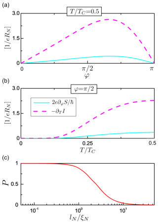
Figure 2: Inconsistency of the Maxwell relation with the rigid boundary condition approximation, using Eqs. (2),(7). (a) Left and right-hand sides of Eq. (11) vs. $\varphi$, at fixed temperature $T=0.5T_{c}$, for $\sigma_{S}A_{S}=\sigma_{N}A_{N}$ and $L_{N}=\xi_{N}$. (b) Same vs. temperature at $\varphi=\pi/2$. (c) The relative discrepancy $P$ (see text) as a function of the normal region size $L_{N}/\xi_{N}$.

The magnitude of the discrepancy in the rigid boundary condition approximation is shown in Fig. 2(a,b), showing the that the left and right-hand sides of Eq. (11) do not match, as functions of phase difference $\varphi$ and temperature $T$. Fig. 2(c) shows the dependence on $L_{N}/\xi_{N}$ of the relative discrepancy

$$P=\max_{(\varphi,T)}\left|\frac{\partial_{T}I+\frac{2e}{\hbar}\partial_{\varphi}S}{\partial_{T}I}\right|\,.$$ (12)

It decreases with increasing junction length $L_{N}$, and remains significant up to $L_{N}$ several times the coherence length $\xi_{N}$. As one would expect, the discrepancy becomes negligible for long junctions ($L_{N}\gg\xi_{N}$).

Let us now point out a mathematical relation between Eqs. (2) and (4) related to the discrepancy. Consider a modified Eilenberger functional, $\mathcal{L}_{\zeta}=\mathcal{L}\rvert_{\omega_{n}\mapsto\omega_{n}+i\zeta}$, where the $\omega_{n}$ appearing explicitly in $\mathcal{L}$ are replaced by $\omega_{n}+i\zeta$, (cf. Ref. Burkhardt and Rainer, 1994) and define the corresponding Green functions $\hat{g}_{\zeta}$ satisfying $\delta{}{\cal F}/\delta\hat{g}\rvert_{\hat{g}_{\zeta}}=0$ and keep $\Delta$ fixed. Recall that the analytic continuation of the sign function is given by $\mathop{\mathrm{sgn}}{}z=z/\sqrt{z^{2}}=\mathop{\mathrm{sgn}}\mathop{\mathrm{Re}}{}z$. The stationary value of the functional then satisfies for real $\zeta$

$$\frac{\mathrm{d}\,}{\mathrm{d}\zeta\,}\mathcal{F}_{S,\zeta}\rvert_{\hat{g}_{\zeta},\Delta}=\pi{}T{\cal N}_{0}\sum_{\omega_{n}}\operatorname{tr}[\mathop{\mathrm{sgn}}(\omega_{n})-\tau_{3}\hat{g}_{\zeta}(i\omega_{n})]\\ =-{\cal N}_{0}\int_{-\infty}^{\infty}\mathrm{d}E\,[N_{\zeta}(E)-1]\tanh\frac{E}{2T}\,.$$ (13)

The second line follows by standard analytic continuation, where $N_{\zeta}(E)=\frac{1}{4}\operatorname{tr}\tau_{3}[g_{\zeta}(E+i0^{+})-g_{\zeta}(E-i0^{+})]$. Suppose now that the boundary conditions are energy-indepenent, i.e., invariant under transformation $\omega_{n}\mapsto{}\omega_{n}+i\zeta$ of explicit frequency arguments: in this case $\hat{g}_{\zeta}(i\omega_{n})=\hat{g}(i\omega_{n}-\zeta)$ and $N_{\zeta}(E)=N(E-\zeta)$ coincide with the energy-shifted Green function and the corresponding DOS. It is worth to notice that $\mathcal{F}_{S,\zeta}\to\text{const}(T)$ for $\zeta\to\infty$ while $\hat{g}(i\omega_{n}-\zeta)\to\tau_{3}\mathop{\mathrm{sgn}}(\omega_{n})$. Moreover, recalling the relation

$$\int_{-\infty}^{0}\mathrm{d}\zeta\,\frac{\mathrm{d}missing\,}{\mathrm{d}T\,}\tanh\frac{E+\zeta}{2T}\\ =-2[f(E,T)\ln{}f(E,T)+(1-f(E,T))\ln(1-f(E,T))]~{},$$ (14)

it follows that $\partial_{T}\mathcal{F}_{S}=-\mathcal{S}_{S}$. Finally, setting $\Delta$ to its self-consistent value (which is a saddle point of $\mathcal{F}_{S}$), we find Eqs. (2) and (4) are equivalent, under the assumption that the boundary conditions do not depend on energy.

The boundary value $\hat{g}_{S,\mathrm{BCS}}(i\omega_{n})$ however is strongly energy dependent, which breaks the above argument and causes the discrepancy between Eqs. (2) and (4),(7). It is interesting to note that a similar issue does not occur in an NSN structure under an analogous approximation (also inspected numerically; not shown), because in that case the value $\hat{g}_{N}=\tau_{3}\mathop{\mathrm{sgn}}\omega_{n}$ imposed in the boundary condition is invariant under $\omega_{n}\mapsto{}\omega_{n}+i\zeta$. This happens also for insulating interfaces ($\hat{n}\cdot\hat{\nabla}\hat{g}=0$) or for periodic boundary conditions, which are functionals of $\hat{g}$ with no explicit dependence on $\omega_{n}$.

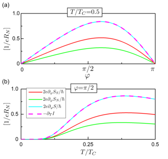
Figure 3: Maxwell relation including the inverse proximity effect. (a) Left and right-hand sides of Eq. (11) vs. $\varphi$, for $T=0.5T_{c}$, $\sigma_{S}A_{S}=\sigma_{N}A_{N}$, $L_{N}=\xi_{N}$. The entropy contributions from the N and S regions, $S=S_{S}+S_{N}$, are also shown separately. (b) Same vs. temperature at $\varphi=\pi/2$.

The apparent thermodynamic discrepancy can be eliminated by properly taking into account the inverse proximity effect. For example, replacing the rigid superconducting terminals by S wires of length $L_{S}$. Below, we adopt a S’SNSS’ geometry, with the boundary conditions $\hat{g}\rvert_{x=-L_{S}}=\hat{g}\rvert_{x=L_{N}+L_{S}}=\hat{g}\rvert_{\mathrm{BCS}}$. The effect of the boundary values is rapidly suppressed and vanishes in the limit $L_{S}\to\infty$.

We show results for such SS’NS’S structure in Fig. 3. In them, the Maxwell relation (11) applies for any $L_{N}$. For simplicity, this calculation does not use a self-consistent $\Delta$, so that the phase derivative is to be understood as explained below Eq. (7). Note that the entropy contribution from the superconductor regions dominates for the parameters chosen.

IV Inverse proximity effect

Let us consider the inverse proximity effect in more detail. We define the entropy difference $\delta S_{S}$ due to the inverse proximity effect in the superconducting region as:

$$\delta S_{S}=S_{S}-S_{{\rm BCS}}=\\ =-4\int^{\infty}_{-\infty}\mathrm{d}E\,\int_{S}\mathrm{d}x\,{\cal N}_{0,S}\delta N(E,x,\varphi)f(E,T)\ln f(E,T)\,,$$ (15)

where ${S}_{{\rm BCS}}$ is the entropy of a bulk BCS superconductor and $\delta N(E,x,\varphi)=N(E,x,\varphi)-N_{{\rm BCS}}(E)$ is the difference of the local density of states from the BCS expression. Moreover, we define dimensionless parameters

$$a=\sigma_{S}A_{S}/(\sigma_{N}A_{N})\,,\qquad\ell=L_{N}/\xi_{N}$$ (16)

for the discussion below.

Analytical solutions can be obtained in the limiting cases of short junction $\ell\ll 1$ at phase differences $\varphi=0$ and $\varphi=\pi$. A solution to the Usadel equation in a semi-infinite superconducting wire with uniform $\Delta=\pm|\Delta|$ is given by

$$\hat{g}=\tau_{3}\cosh\theta+i\tau_{2}\sinh\theta$$ (17)

where (cf. Ref. Zaikin and Zharkov, 1981)

$$\theta(x)=\theta_{S}-4\operatorname{artanh}\Bigl{(}e^{-\sqrt{2}(x-L_{N})/\xi_{E}}\tanh\frac{\theta_{S}-\theta(L_{N})}{4}\Bigr{)}\,,$$ (18)

and $\xi_{E}=(1-E^{2}/|\Delta|^{2})^{-1/4}\xi_{N}$ and $\theta_{S}=\operatorname{artanh}\frac{|\Delta|}{E+i0^{+}}$. The spatially integrated change in the superconductor DOS can be evaluated based on this solution:

$$\int_{S}\mathrm{d}x\,\delta N(x,E)=\\ =\sqrt{2}\mathop{\mathrm{Re}}\Bigl{[}\xi_{E}\cosh\theta_{S}\bigl{(}\cosh\frac{\theta_{S}-\theta(L_{N})}{2}-1\bigr{)}+\qquad\\ -\xi_{E}\sinh\theta_{S}\sinh\frac{\theta_{S}-\theta(L_{N})}{2}\Bigl{]}$$ (19)

For $L_{N}\ll\xi_{E}$, the Usadel equation in the N region can be approximated as $\partial_{x}^{2}\theta(x)=0$. Matching to the boundary condition $\sigma_{N}A_{N}\partial_{x}\theta_{N}=\sigma_{S}A_{S}\partial_{x}\theta_{S}$ at the two NS interfaces results to

$$\theta(L_{N})=\begin{cases}\theta_{S}&\text{for $\varphi=0$,}\\ \sqrt{2}\frac{\xi_{E}}{\xi_{N}}a\ell\sinh\frac{\theta_{S}-\theta(L_{N})}{2}&\text{for $\varphi=\pi$}\,,\end{cases}$$ (20)

from which $\theta(L_{N})$ can be solved. For the entropy at $\varphi=0$, this gives a trivial solution $\delta S_{S}=0$. On the other hand, at $\varphi=\pi$, we have for temperatures $T\ll|\Delta|$,

$$\delta{}S_{S}(\varphi=\pi)\simeq\frac{4\pi^{2}}{3}T{\cal N}_{0,S}A_{S}\xi_{N}\times\begin{cases}1\,,&\text{for $a\ell\ll 1$,}\\ \frac{\pi}{2a\ell}\,,&\text{for $a\ell\gg 1$.}\end{cases}$$ (21)

The full temperature dependence for $\ell\to 0$ reads

$$\delta{}S_{S}(\varphi=\pi)=-\frac{16}{\sqrt{2}}{\cal N}_{0,S}A_{S}\int_{-\infty}^{\infty}\mathrm{d}E\,f(E,T)\ln f(E,T)\\ \quad\times\mathop{\mathrm{Re}}[(\cosh\frac{\theta_{S}}{2}-\cosh\theta_{S})\xi_{E}]\,.$$ (22)

For cross-over regions, the boundary condition matching would need to be solved numerically.

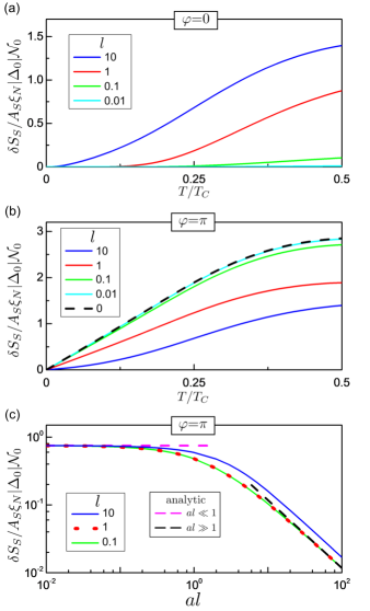
Figure 4: Behavior of the entropy variation $\delta S_{S}$ of the superconducting leads. (a) Temperature dependence at $\varphi=0$ for $a=1$ and different $\ell$. (b) Same at $\varphi=\pi$. Result (22) for $\ell=0$ is also shown (dashed). (c) Dependence of $\delta S_{S}(\varphi=\pi)$ on $\ell$ and $a$, at $T/T_{C}=0.1$. Limiting behavior from Eq. (21) is indicated (dashed).

The behavior in the rigid boundary condition limit (i.e. $a\to\infty$) can be understood based on the above result. For the entropy, the short-junction rigid-boundary limit $a\to\infty$, $\ell\to 0$ is not unique, but results depend on the product $a\ell$. Generally, the entropy is proportional to $\hbar/(e^{2}R_{\rm tot})$, where $R_{\rm tot}$ is the resistance of $\xi_{S}$-length superconductor segment in series with the normal wire, as can be expected a priori Likharev (1979).

Figures 4(a,b) show the geometry dependence of the proximity effect contribution $\delta{S}_{S}$ to the entropy, for $\varphi=0$ and $\varphi=\pi$. Generally, $\delta S_{S}(\varphi=0)$ decreases with decreasing junction length and approaches the limit of $\delta S_{S}(\varphi=0)\rightarrow 0$ for $l\rightarrow 0$. The temperature dependence of $\delta{S}_{S}(0)$ is largely affected by the presence of a minigap in the spectrum, $S(0)\sim{}e^{-E_{g}/T}$ with $E_{g}\sim{}\min[\hbar{}D_{N}/L_{N}^{2},|\Delta|]$ [see Fig. 1(b)]. For $\varphi=\pi$ on the other hand, the entropy contribution $\delta S_{S}$ of the superconductors increases with decreasing length, in accordance with the increase of the supercurrent with decreasing junction resistance. For very short junctions, $\ell\lesssim{}a^{-1}$, $\delta S_{S}$ saturates as indicated in Eq. (21). The behavior of $\delta S_{S}(\varphi=\pi)$ at phase difference $\varphi=\pi$ as a function of the product $al$ is shown in Fig. 4(c). It is interesting to note that the results are essentially converged to the short-junction limit $l\ll 1$ already at $l=1$.

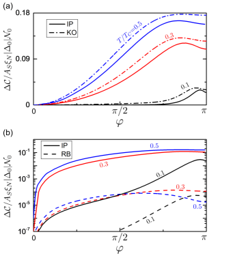
Figure 5: Modulation of the heat capacity $\Delta C(T,\varphi)=C(T,\varphi)-C(T,\varphi=0)$ in an SNS junction, for $a=500$, $\ell=0.1$. (a) Numerical results including inverse proximity effect (IP, solid) and results from Eq. (9) (KO, dash-dotted), for different temperatures. (b) Same, shown on a logarithmic scale, together with the result from a rigid boundary condition approximation (RB, dashed).

V Heat capacity

The heat capacity

$$C=T\frac{\mathrm{d}S\,}{\mathrm{d}T\,}\,,$$ (23)

can be obtained from the entropy discussed in the previous sections. Fig. 5 shows numerical results for the heat capacity. In these calculations, the order parameter $\Delta(x,T)$ is computed to satisfy the self-consistency relations $\delta{}F/\delta\Delta=\delta{}F/\delta\Delta^{*}=0$. For the selected short junction length, $al\gg 1$, and the numerical results obtained by taking the inverse proximity effect into account match relatively well with Eq. (9). Note that a self-consistent $\Delta$ does not cause significant qualitative deviations. On the other hand, calculations within the rigid boundary condition approximation, shown in Fig. 5(b), underestimate the heat capacity by several orders of magnitude. As pointed out above, we expect that this approach is accurate only for long junctions $L_{N}\gtrsim{}5\xi_{N}$.

Finally, note that the total heat capacity at $\varphi=0$, being an extensive quantity, will generally depend on device parameters of the whole system.

VI Summary and discussion

The entropy in SNS junctions roughly consists of two contributions — a phase dependent part associated with the bound states contributing also to the supercurrent, and a phase-independent part. Generally, the two behave differently as a function of the junction length. Moreover, the phase-dependent contribution in short junctions, if expressed in terms of the local density of states, largely originates from the proximity effect in the superconducting banks. Approximations that neglect this can produce thermodynamically inconsistent results. The results also reiterate, as clear from the connection to CPR, that the junction heat capacity has a part not directly related to the junction volume. A proper quantitative calculation of entropy and thermodynamic quantities taking into account inverse proximity effect is thus of importance both for fundamental and application purposes.

Finally, we can consider factors important for an experimental measurement of the heat capacity of a single nanoscale SNS junction. For example, the heat capacity of the junction can be inferred by measuring the temperature variation, after an heating pulse, as a function of the phase difference, which can be manipulated by means of external field. For such experimental realization, two points have to be considered with care. First, the device should be thermally well-isolated, in order to avoid heat dispersion outside of device volume itself. Second, the bulk superconductor mass should be made as small as possible: the total heat capacity $C$ is an extensive property, so its variation as a function of phase difference $\Delta C(\varphi)/C$ increases by increasing the ratio of critical current and device volume. However, this target will be also constrained by the requirement of large superconducting leads in order to ensure the phase-bias of the junction and thus an optimal trade-off has to be considered in a proper device design.

In summary, we discussed entropy and heat capacity in SNS structures numerically and analytically, and point out that inconsistencies appear if inverse proximity contributions are not properly included. The results obtained can be used in designing superconducting devices concerning caloritronic, heat and photon sensors, and are in general relevant also for other devices based on thermodynamic working principles.