Is completeness necessary? Estimation in nonidentified linear models

Abstract

We show that estimators based on spectral regularization converge to the best approximation of a structural parameter in a class of nonidentified linear ill-posed inverse models. Importantly, this convergence holds in the uniform and Hilbert space norms. We describe several circumstances when the best approximation coincides with a structural parameter, or at least reasonably approximates it, and discuss how our results can be useful in the partial identification setting. Lastly, we document that identification failures have important implications for the asymptotic distribution of a linear functional of regularized estimators, which can have a weighted chi-squared component. The theory is illustrated for various high-dimensional and nonparametric IV regressions.

Keywords: completeness condition, weak identification, nonparametric IV regression, high-dimensional regressions, spectral regularization.
JEL Classifications: C14, C26

1 Introduction

Structural nonparametric and high-dimensional models are often ill-posed. Among many examples, we may quote the nonparametric IV regression, various high-dimensional regressions, measurement errors, and random coefficient models. All these examples lead to the ill-posed functional equation

$$K\varphi=r,$$

where $\varphi$ is a structural parameter of interest, $r$ is a function, and $K$ is a linear operator. The classical numerical literature on ill-posed inverse problems, see Engl, Hanke, and Neubauer (1996), studies deterministic problems, where the operator $K$ is usually known and $r$ is measured with a deterministic numerical error. In econometric applications, both $K$ and $r$ are estimated from the data, and we are faced with the statistical ill-posed inverse problems.

Identification is an integral part of econometric analysis, going back to Koopmans (1949), Koopmans and Reiersol (1950), and Rothenberg (1971) in the parametric case. In nonparametric and high-dimensional ill-posed inverse problems, $K$ and $r$ are directly identified from the data-generating process, while the structural parameter $\varphi$ is identified if the equation $K\varphi=r$ has a unique solution. The uniqueness is equivalent to assuming that $K$ is a one-to-one operator, or in other words that $K\phi=0\implies\phi=0$ for all $\phi$ in the domain of $K$. It is worth stressing that the operator $K$ is usually unknown in econometric applications and the estimated operator $\hat{K}$ has a finite rank and is not one-to-one for every finite sample size.

The maximum likelihood estimator when there is a lack of identification leads to a flat likelihood in some regions of a parameter space and then to the ambiguity on the choice of a maximum. It is then natural to characterize the limit of an estimator for such a potentially nonidentified model. In the nonidentified ill-posed inverse models, the identified set is an linear manifold $\phi+\mathcal{N}(K)$, where $\phi$ is any solution to $K\phi=r$, and $\mathcal{N}(K)$ is the null space of $K$. Note that the identified set is in general unbounded and is not informative on the structural parameter $\varphi$ without additional constraints.

As $K$ or $\hat{K}$ may fail to be one-to-one and typically have a discontinuous generalized inverse, some regularization is needed to estimate consistently the structural parameter. In this paper, we focus on spectral regularization methods consisting of modifying the spectrum of the operator $\hat{K}$. Tikhonov regularization, also known as functional ridge regression, is one prominent example; see Tikhonov (1963). Other important instances of spectral regularizations include the iterated Tikhonov; the spectral cut-off, which is also related to the functional principal component analysis, see Yao, Müller, and Wang (2005); and the Landweber-Fridman, which is also related to the functional gradient descent. We show that estimators based on the spectral regularization are uniformly consistent for the best approximation to the structural parameter in the orthogonal complement to the null space of the operator and study the distributional consequences of identification failures.

In some cases, the best approximation may coincide with the structural parameter or at least may reasonably approximate it, even when the operator $K$ has a non-trivial null space. This provides an attractive interpretation for the nonparametric IV regression under identification failures similar in a way to the best approximation property of least-squares under misspecifications; see Angrist and Pischke (2008), Chapter 3. Lastly, the best approximation can also be used in the partial identification approach.

Contribution and related literature.

There exists a large literature on the spectral regularization of statistical inverse problems; see Carrasco, Florens, and Renault (2007, 2014), Darolles, Fan, Florens, and Renault (2011), Florens, Johannes, and Van Bellegem (2011), Gagliardini and Scaillet (2012), and Babii (2020) among others. With an exception for Florens, Johannes, and Van Bellegem (2011) and Chen and Pouzo (2012), the existing literature does not study the consequences of identification failures. In particular, related to our work, Florens, Johannes, and Van Bellegem (2011) derive the convergence rates of Tikhonov regularization to the best approximation in the $L_{2}$ norm when the operator is known and extend this result to the case of unknown operator under some high-level conditions on the regularization parameter and moments of the estimation error. However, these conditions have not been verified for specific models, such as the nonparametric IV or various high-dimensional regressions.

Our original contributions to this literature are to show that 1) the convergence to the best approximation holds in the $L_{\infty}$ norm when Tikhonov regularization is used; 2) the convergence holds for general spectral regularizations in the $L_{\infty}$ and Hilbert space norms under low-level and easy-to-verify conditions; 3) the asymptotic distribution of linear functionals can transition between the Gaussian and chi-squared limits under identification failures. These results are illustrated for various high-dimensional regressions and the nonparametric IV regression.

Our paper also relates to the identification literature in the special case of nonparametric IV regression, see Newey and Powell (2003), D’Haultfoeuille (2011), Canay, Santos, and Shaikh (2013), Andrews (2017), Freyberger (2017), Hu and Shiu (2018), and more generally other ill-posed inverse models encountered in econometrics. In particular, our results on the consistency to the best approximation in the $L_{\infty}$ norm in conjunction with Freyberger (2017) can be used to obtain the set estimators under identification failures.

It is also worth emphasizing that our general theory is not limited by the nonparametric IV regression and can potentially be applied to other ill-posed inverse models such as measurement errors, see Hu and Schennach (2008); dynamic models with unobserved state variables, see Hu and Shum (2012); demand models, see Berry and Haile (2014) and Dunker, Hoderlein, and Kaido (2017); neoclassical trade models, see Adao, Costinot, and Donaldson (2017); models of earnings and consumption dynamics, see Arellano, Blundell, and Bonhomme (2017) and Botosaru (2019); structural random coefficient models, see Hoderlein, Nesheim, and Simoni (2017); discrete games, see Kashaev and Salcedo (2020); models of two-sided markets, see Sokullu (2016); high-dimensional mixed-frequency IV regressions, see Babii (2021) and various functional regressions, see Florens and Van Bellegem (2015) and Benatia, Carrasco, and Florens (2017); and endogenous sample selection models, see Breunig, Mammen, and Simoni (2018). Related identification issues also appear in quantile treatment effect models, see Chernozhukov and Hansen (2005), and nonlinear asset pricing models, see Chen and Ludvigson (2009) and Chen, Pelger, and Zhu (2020).

The paper is organized as follows. Section 2 discusses the identification in linear ill-posed inverse models using the nonparametric IV and various high-dimensional regressions as leading examples. In Section 3, we obtain the non-asymptotic risk bounds in the $L_{\infty}$ and the Hilbert space norms for a class of Tikhonov-regularized estimators, which are extended to general regularization schemes in the Appendix Section A.1. Section 4 illustrates how these results can be applied to the partial identification. In the Appendix Section A.2, we show that in the extreme case of identification failures, the Tikhonov-regularized estimator is driven by the degenerate U-statistics in large samples. Building on these results, we illustrate in Section 5 the transition between the Gaussian and the weighted chi-squared asymptotics in the intermediate cases. We report on a Monte Carlo study in Section 6 which provides further insights about the validity of our asymptotic results in finite sample settings typically encountered in empirical applications. Section 7 concludes. All proofs are collected in the Appendix Section A.3. We also review several relevant results from the theory of the generalized inverse operators and the theory of the Hilbert space valued U-statistics in the Online Appendix Sections B.1 and B.2.

2 Identification

Consider the functional linear equation

$$K\varphi=r,$$

where $K:\mathcal{E}\to\mathcal{H}$ is a compact linear operator, defined on some Hilbert spaces $\mathcal{E}$ and $\mathcal{H}$, and $\varphi\in\mathcal{E}$ is a structural parameter of interest. The structural parameter $\varphi$ is point identified if the operator $K$ is one-to-one, or in other words if the null space of $K$, denoted $\mathcal{N}(K)=\left\{\phi\in\mathcal{E}:\;K\phi=0\right\}$, reduces to $\{0\}$. Equivalently, the point identification of $\varphi$ requires that

$$K\phi=0\implies\phi=0,\qquad\forall\phi\in\mathcal{E}.$$

We illustrate the statistical interpretation of the one-to-one property of $K$ in the nonparametric IV regression and the high-dimensional regressions.

Example 2.1 (Nonparametric IV regression).

Consider

$$Y=\varphi(Z)+U,\qquad\mathds{E}[U|W]=0,$$

where $(Y,Z,W)\in\mathbf{R}\times\mathbf{R}^{p}\times\mathbf{R}^{q}$ is a random vector, see Darolles, Fan, Florens, and Renault (2011). The exclusion restriction leads to the functional linear equation

$$r(w)\triangleq\mathds{E}[Y|W=w]=\mathds{E}[\varphi(Z)|W=w]\triangleq(K\varphi)(w),$$

where $K:L_{2}(Z)\to L_{2}(W)$ is a conditional expectation operator. The completeness condition, or more precisely the $L_{2}$-completeness, see Florens, Mouchart, and Rolin (1990) and Newey and Powell (2003), is the one-to-one property of the conditional expectation operator

$$\mathds{E}[\phi(Z)|W]=0\implies\phi=0,\qquad\forall\phi\in L_{2}(Z).$$

It is a (non-linear) dependence condition between the endogenous regressor $Z$ and the instrument $W$.

Example 2.2 (High-dimensional regressions).

Consider

$$Y=\langle Z,\varphi\rangle+U,\qquad\mathds{E}[UW]=0,$$

where $(Y,Z,W)\in\mathbf{R}\times\mathcal{E}\times\mathcal{H}$, see Florens and Van Bellegem (2015). The exclusion restriction leads to the functional linear equation

$$r\triangleq\mathds{E}[YW]=\mathds{E}[\langle Z,\varphi\rangle W]\triangleq K\varphi,$$

where $K:\mathcal{E}\to\mathcal{H}$ is a covariance operator. The completeness condition is a one-to-one property of the covariance operator

$$\mathds{E}[\langle Z,\phi\rangle W]=0\implies\phi=0,\qquad\forall\phi\in\mathcal{E}.$$

It generalizes the rank condition used in the linear IV regression and requires a sufficient (linear) dependence between $Z$ and $W$.

If the completeness condition fails, then the null space of the operator $K$ is a non-trivial closed linear subspace of $\mathcal{E}$ and the structural parameter $\varphi$ is only set identified. The identified set is a closed linear manifold

$$\Phi^{\mathrm{ID}}=\varphi+\mathcal{N}(K),$$

where $\mathcal{N}(K)$ is the null space of $K$. The identified set is in general unbounded, however, practical applications also involve some smoothness restrictions under which the identified set can be bounded.

Since $\mathcal{N}(K)$ is a closed linear subspace of $\mathcal{E}$, decompose

$$\varphi=\varphi_{1}+\varphi_{0},$$

where $\varphi_{1}$ is the unique projection of $\varphi$ on $\mathcal{N}(K)^{\perp}$ and $\varphi_{0}$ is the orthogonal projection of $\varphi$ on $\mathcal{N}(K)$. By orthogonality, $\|\varphi\|^{2}=\|\varphi_{1}\|^{2}+\|\varphi_{0}\|^{2}\geq\|\varphi_{1}\|^{2}$. Therefore, $\varphi_{1}$ has a smaller norm than $\varphi$, with the two being equal when $\varphi_{0}=0$. Since $\mathcal{N}(K)^{\perp}=\overline{\mathcal{R}(K^{*})}$, see Luenberger (1997), p.157, the best approximation $\varphi_{1}$ equals to the structural parameter $\varphi$ whenever the structural parameter $\varphi$ belongs to $\overline{\mathcal{R}(K^{*})}$. This condition has also an appealing regularity interpretation known as the source condition. To see this, note that $\mathcal{R}(K^{*})=\mathcal{R}(K^{*}K)^{1/2}$; see Engl, Hanke, and Neubauer (1996), Proposition 2.18. Therefore, if the ill-posed inverse problem has a sufficiently high regularity, so that $\varphi\in\mathcal{R}(K^{*}K)^{\beta/2}$ with $\beta\in[1,\infty)$, then $\varphi_{1}=\varphi$, and the structural function $\varphi$ is point identified although the completeness condition fails.

The best approximation is also be informative, whenever the structural function $\varphi$ can be well approximated by the family of basis functions of $\mathcal{N}(K)^{\perp}$. The following example illustrates this further for the nonparametric IV regression.

Example 2.3 (Nonparametric IV regression).

Suppose that the conditional expectation operator

$$K:L_{2}(Z) \to L_{2}(W)$$

$$\phi \mapsto\mathds{E}[\phi(Z)|W]$$

is compact. By the spectral theorem, there exists $(\lambda_{j},\varphi_{j},\psi_{j})_{j\geq 1}$, where $\lambda_{j}\to 0$ is a sequence of singular values, $(\varphi_{j})_{j\geq 1}$ is a complete orthonormal system of $\mathcal{N}(K)^{\perp}=\overline{\mathcal{R}(K^{*})}$, and $(\psi_{j})_{j\geq 1}$ is the complete orthonormal system of $\mathcal{N}^{\perp}(K^{*})=\overline{\mathcal{R}(K)}$. The best approximation coincides with the structural function $\varphi$, whenever it can be represented in terms of the family $(\varphi_{j})_{j\geq 1}$.

It is also known that the completeness condition fails in the nonparametric IV regression when $Z$ has the Lebesgue density while the instrumental variable is a discrete random variable. The following example illustrates that if the instrumental variable $W$ takes a sufficiently large number of discrete values, then the function $\varphi$ might be accurately estimated even if the completeness condition fails.

Example 2.4 (Nonparametric IV with discrete instrument).

Consider the nonparametric IV regression with a discrete instrumental variable $W\in\{w_{k}:\;k\geq 1\}$. Put $f_{k}(z)=f_{Z|W=w_{k}}(z)$ for every $k\geq 1$. Then

$$\mathcal{N}(K)=\left\{\phi\in L_{2}(Z):\>\langle\phi,f_{k}\rangle=0,\;\forall k\geq 1\right\}$$

and if $\varphi\in\mathrm{span}\{f_{k}:\;k\geq 1\}$, then $\varphi\in\mathcal{N}(K)^{\perp}$. The best approximation coincides with the structural parameter $\varphi$ whenever it can be represented in terms of the family $(f_{k})_{k\geq 1}$.

It is worth stressing that functions encountered in empirical settings can typically be well-approximated by a fairly small number of series terms, in which case even if $\varphi$ cannot be exactly represented by families $(\varphi_{j})_{j\geq 1}$ or $(f_{k})_{k\geq 1}$, these families could capture most of the nonlinearities; see also Section 4 for a partial identification perspective.

3 Nonasymptotic risk bounds

In this section, we derive the nonasymptotic risk bounds for the Tikhonov-regularized estimator in the Hilbert space and the uniform norms. All results will be stated uniformly over the relevant class of models without relying on the completeness condition.

3.1 Tikhonov-regularized estimator

Estimation of the structural function $\varphi$ is an ill-posed inverse problem and requires regularization for two reasons. First, the generalized inverse of $K$ is typically not continuous; see Appendix B.1. Second, the estimator $\hat{K}$ is typically a finite-rank operator and is not one-to-one for any finite sample size.

The Tikhonov-regularized estimator solves the following penalized least-squares problem

$$\min_{\phi}\left\|\hat{K}\phi-\hat{r}\right\|^{2}+\alpha_{n}\|\phi\|^{2},$$

where $\alpha_{n}>0$ is a regularization parameter. It is easy to see that the solution to this problem is

$$\hat{\varphi}=(\alpha_{n}I+\hat{K}^{*}\hat{K})^{-1}\hat{K}^{*}\hat{r}.$$

The estimator enjoys two fundamental properties:

1. It is well-defined even when $K$ or $\hat{K}$ is not one-to-one.

2. If $\alpha_{n}\to 0$ at an appropriate rate, it converges to the best approximation to $\varphi$ in $\mathcal{N}(K)^{\perp}$.

Indeed, even if $\hat{K}^{*}\hat{K}$ had an eigenvalue $\hat{\lambda}_{j}=0$, the corresponding eigenvalue of $\alpha_{n}I+\hat{K}^{*}\hat{K}$ would be $\alpha_{n}+\hat{\lambda}_{j}>0$ with a well-defined inverse. In the following two sections, we show that 2. holds in the Hilbert space and the uniform norms.

3.2 Hilbert space risk

First, we describe the relevant class of structural functions and operators:

Assumption 3.1.

The structural parameter $\varphi=\varphi_{1}+\varphi_{0}$ and the operator $K$ are in

$$\mathcal{F}(\beta,C)=\left\{(\varphi,K):\;\varphi_{1}=(K^{*}K)^{\beta/2}\psi,\;\|\psi\|^{2}\vee\|\varphi_{0}\|\vee\|K\|\leq C\right\}$$

for some $\beta,C>0$, where $\|K\|=\sup_{\|\phi\|\leq 1}\|K\phi\|$ and $a\vee b=\max\{a,b\}$.

To illustrate this assumption, let $(\sigma_{j},e_{j},h_{j})_{j\geq 1}$ be the SVD decomposition of $K:\mathcal{E}\to\mathcal{H}$; see Kress (2014), Theorem 15.16. Then $\varphi_{1}=\sum_{j\geq 1}\langle\varphi_{1},e_{j}\rangle e_{j}$ and by the Parseval’s identity since $\psi=(K^{*}K)^{-\beta/2}\varphi_{1}$

$$\|\psi\|^{2}=\sum_{j\geq 1}\frac{|\langle\varphi_{1},e_{j}\rangle|^{2}}{\sigma_{j}^{2\beta}}.$$

Therefore, Assumption 3.1 restricts the relative rates of decline of singular values $(\sigma_{j})_{j\geq 1}$, describing the ill-posedness and Fourier coefficients $\langle\varphi_{1},e_{j}\rangle_{j\geq 1}$, describing the regularity of $\varphi_{1}$.

We estimate $(r,K)$ with $(\hat{r},\hat{K})$ and make the following assumption:

Assumption 3.2.

(i) $\mathds{E}\|\hat{r}-\hat{K}\varphi_{1}\|^{2}\leq C_{1}\delta_{n}$; and (ii) $\mathds{E}\|\hat{K}-K\|^{2}\leq C_{2}\rho_{1n},$ where $C_{1},C_{2}<\infty$ do not depend on $(\varphi,K)$ and $\delta_{n},\rho_{1n}\to 0$ as $n\to\infty$.

Assumption 3.2 describes the convergence rate of residuals and the estimated operator. Note also that the residuals in the nonidentified model, $\hat{r}-\hat{K}\varphi_{1}$, can be written as a sum of identified residuals $\hat{r}-\hat{K}\varphi$ and $\hat{K}\varphi_{0}$ which can be controlled separately.

The following result holds for the Hilbert space norm:

Theorem 3.1.

Suppose that Assumptions 3.1 and 3.2 are satisfied. Then for all $\beta\in(0,2]$

$$\sup_{(\varphi,K)\in\mathcal{F}}\mathds{E}\left\|\hat{\varphi}-\varphi_{1}\right\|^{2}=O\left(\frac{\delta_{n}+\rho_{1n}\alpha^{\beta\wedge 1}}{\alpha_{n}}+\alpha^{\beta}_{n}\right),$$

where $a\wedge b=\max\{a,b\}$.

Theorem 3.1 shows that the convergence rate in the Hilbert space norm is driven by the rates of:

• residuals of order $O\left(\delta_{n}/\alpha_{n}\right)$;

• estimated operator of order $O\left(\rho_{1n}\alpha^{\beta\wedge 1}/\alpha_{n}\right)$;

• the regularization bias of order $O\left(\alpha_{n}^{\beta}\right)$.

It is worth mentioning a stronger version of Assumption 3.1 is commonly assumed: $\varphi\in\mathcal{R}(K^{*}K)^{\beta/2}$ with $\beta\geq 1$; see Carrasco, Florens, and Renault (2007). In this case, we actually have $\varphi_{0}=0$ and the Tikhonov regularized estimator can estimate consistently the structural parameter $\varphi$, despite the fact that the completeness condition fails. More generally, we distinguish the following possibilities:

• identified case: $\varphi_{0}=0$ and $\rho_{1n}\alpha^{\beta\wedge 1}\lesssim\delta_{n}$, where the convergence rate to $\varphi$ is driven by residuals $\hat{r}-\hat{K}\varphi$;

• weakly identified case: $\varphi_{0}=0$ and $\delta_{n}\lesssim\rho_{1n}\alpha^{\beta\wedge 1}$, where the convergence rate to $\varphi$ is driven by the estimated operator $\hat{K}$;

• nonidentified case: $\varphi_{0}\neq 0$ and $\rho_{1n}\alpha^{\beta\wedge 1}\lesssim\delta_{n}$, where the convergence rate to $\varphi_{1}$ is driven by residuals $\hat{r}-\hat{K}\varphi_{1}$;

• strongly nonidentified models: $\varphi_{0}\neq 0$ and $\delta_{n}\lesssim\rho_{1n}\alpha^{\beta\wedge 1}$, where the convergence rate to $\varphi_{1}$ is driven by the estimated operator $\hat{K}$.

In the identified case, the optimal choice of the regularization parameter is $\alpha_{n}\sim\delta_{n}^{1/(\beta+1)}$, which leads to the optimal convergence rate of order $O\left(\delta_{n}^{\beta/(\beta+1)}\right)$ for the class $\mathcal{F}(\beta,C)$ with $\beta\in(0,2]$; see Mair and Ruymgaart (1996). The rate is not optimal for $\beta>2$, but we show in the Appendix Section A.1 that the optimal rate can be achieved with additional iterations or some alternative regularization schemes.

Lastly, it is worth mentioning that in the special case of $L_{2}$ spaces, Theorem 3.1 provides a sharper result than Florens, Johannes, and Van Bellegem (2011), Theorem 2.2, where the rate is always driven by $\rho_{1n}$.

3.3 $L_{\infty}$ risk

Suppose now that the space of continuous functions on a compact set $D\subset\mathbf{R}^{p}$, denoted $(C(D),\|.\|_{\infty})$, is embedded into the space $\mathcal{E}$, where $\|.\|_{\infty}$ is the uniform norm. Suppose also that $\mathcal{R}(K^{*})\subset C(D)$ and that $\varphi_{1}\in C(D)$. Let $\|K^{*}\|_{2,\infty}=\sup_{\|\phi\|\leq 1}\|K^{*}\phi\|_{\infty}$ be the mixed operator norm of $K^{*}$. The following assumption describes how well the operator $K^{*}$ is estimated by $\hat{K}^{*}$ in the $\|.\|_{2,\infty}$ norm.

Assumption 3.3.

Suppose that $\|K^{*}\|_{2,\infty}\leq C_{3}$ and that $\mathds{E}\|\hat{K}^{*}-K^{*}\|_{2,\infty}^{2}\leq C_{3}\rho_{2n}$, where $C_{3}<\infty$ does not depend on $(\varphi,K)$ and $\rho_{2n}\to 0$.

The following result holds:

Theorem 3.2.

Suppose that Assumptions 3.1, 3.2, and 3.3 are satisfied with $\varphi_{1}=(K^{*}K)^{\beta/2}K^{*}\psi$. Then for all $\beta\in(0,2]$

$$\sup_{(\varphi,K)\in\mathcal{F}}\mathds{E}\left\|\hat{\varphi}-\varphi_{1}\right\|_{\infty}=O\left(\frac{\delta_{n}^{1/2}+\rho_{1n}^{1/2}\alpha_{n}^{\frac{\beta+1}{2}\wedge 1}+\rho_{2n}^{1/2}\alpha_{n}^{1/2}}{\alpha_{n}}+\alpha_{n}^{\beta/2}\right).$$

Theorem 3.2 describes the uniform convergence rates for generic ill-posed inverse problems. In constrast to Theorem 3.1, the $L_{\infty}$ convergence rate is also driven by the estimation error in $K^{*}$ measured in the $\|.\|_{2,\infty}$ norm. We also obtain the $L_{\infty}$ convergence rate for more general spectral regularization schemes in the Appendix Section A.1.

3.4 Applications

3.4.1 High-dimensional regressions

Following, Example 2.2, the econometrician observes an i.i.d. sample $(Y_{i},Z_{i},W_{i})_{i=1}^{n}$. Then

$$r=\mathds{E}[YW],\qquad K\phi=\mathds{E}[W\langle\phi,Z\rangle],\qquad K^{*}\psi=\mathds{E}[Z\langle\psi,W\rangle]$$

are estimated with

$$\hat{r}=\frac{1}{n}\sum_{i=1}^{n}Y_{i}W_{i},\qquad\hat{K}\phi=\frac{1}{n}\sum_{i=1}^{n}W_{i}\langle Z_{i},\phi\rangle,\qquad\hat{K}^{*}\psi=\frac{1}{n}\sum_{i=1}^{n}Z_{i}\langle W_{i},\psi\rangle.$$

Then the elementary computations give

$$\mathds{E}\left\|\hat{r}-\hat{K}\varphi_{1}\right\|^{2}=\frac{\mathds{E}\|(Y-\langle Z,\varphi_{1}\rangle)W\|^{2}}{n}\qquad\text{and}\qquad\mathds{E}\left\|\hat{K}-K\right\|^{2}\leq\frac{\mathds{E}\|ZW\|^{2}}{n}.$$

Let $\mathcal{F}(\beta,C)$ be the class of models as in the Assumption 3.1 and suppose also that $\mathds{E}\|UW\|^{2}\vee\mathds{E}\|ZW\|^{2}\leq C$ for all models in this class. Then $\delta_{n}=\rho_{1n}=n^{-1}$ and Theorem 3.1 shows that the Hilbert space risk is of order

$$\sup_{(\varphi,K)\in\mathcal{F}}\mathds{E}\left\|\hat{\varphi}-\varphi_{1}\right\|^{2}=O\left(\frac{1}{\alpha_{n}n}+\alpha^{\beta}_{n}\right).$$

The high-dimensional regression is either identified ($\varphi_{0}=0$) or nonidentified ($\varphi_{0}\neq 0$). Then conditions $\alpha_{n}\to 0$ and $\alpha_{n}n\to\infty$ as $n\to\infty$ are sufficient to guarantee the consistency in the Hilbert space norm. In particular, the optimal choice $\alpha_{n}\sim n^{-1/(\beta+1)}$ leads to the convergence rate of order $O(n^{-\beta/(\beta+1)})$.

For the uniform convergence, suppose that $\mathcal{E}=L_{2}(S)$, i.e. a set of functions on some bounded set $S\subset\mathbf{R}^{d}$, square-integrable with respect to the Lebesgue measure. To verify the Assumption 3.3, we also assume that models in $\mathcal{F}(\beta,C)$ are such that $\|Z\|_{\infty}\vee\|W\|_{\infty}\leq C<\infty$ and that stochastic processes $Z$ and $W$ are in some Hölder ball with smoothness $s>d/2$. Then by the Hoffman-Jørgensen and moment inequalities, see Giné and Nickl (2016), p.129 and p.202,

$$\mathds{E}\left\|\hat{K}^{*}-K^{*}\right\|_{2,\infty}^{2}=O\left(\frac{1}{n}\right).$$

Therefore, Assumption 3.3 is satisfied with $\rho_{2n}=n^{-1}$, and Theorem 3.2 shows that

$$\sup_{(\varphi,K)\in\mathcal{F}}\mathds{E}\left\|\hat{\varphi}-\varphi_{1}\right\|_{\infty}=O\left(\frac{1}{\alpha_{n}n^{1/2}}+\alpha_{n}^{\beta/2}\right).$$

Then conditions $\alpha_{n}\to 0$ and $\alpha_{n}n^{1/2}\to\infty$ as $n\to\infty$ ensure the uniform consistency of $\hat{\varphi}$. In particular, the optimal choice $\alpha_{n}\sim n^{-1/(\beta+2)}$ leads to the convergence rate of order $O(n^{-\beta/{(2\beta+4)}})$.

3.4.2 Nonparametric IV regression

Following Example 2.1, rewrite the model as

$$r(w)\triangleq\mathds{E}[Y|W=w]f_{W}(w)=\int\varphi(z)f_{ZW}(z,w)\mathrm{d}z\triangleq(K\varphi)(w),$$

where $K:L_{2}([0,1]^{p})\to L_{2}([0,1]^{q})$. We can estimate $r$ and $K$ via kernel smoothing:

$$\hat{r}(w) =\frac{1}{nh_{n}^{q}}\sum_{i=1}^{n}Y_{i}K_{w}\left(h_{n}^{-1}(W_{i}-w)\right),$$

$$(\hat{K}\phi)(w) =\int\phi(z)\hat{f}_{ZW}(z,w)\mathrm{d}z,$$

$$\hat{f}_{ZW}(z,w) =\frac{1}{nh_{n}^{p+q}}\sum_{i=1}^{n}K_{z}\left(h_{n}^{-1}(Z_{i}-z)\right)K_{w}\left(h_{n}^{-1}(W_{i}-w)\right),$$

where $K_{w}$ and $K_{z}$ are symmetric kernel functions and $h_{n}\to 0$ is a bandwidth parameter. Under mild assumptions, by Proposition A.3.1, $\delta_{n}=\frac{1}{nh^{q}_{n}}+h^{2s}_{n}$ and $\rho_{1n}=\frac{1}{nh^{p+q}_{n}}+h^{2s}_{n}$, where $s$ is the Hölder smoothness of $f_{ZW}$. Therefore, Theorem 3.1 shows that mean-integrated squared error has the following rate

$$\sup_{(\varphi,K)\in\mathcal{F}}\mathds{E}\left\|\hat{\varphi}-\varphi_{1}\right\|^{2}=O\left(\frac{1}{\alpha_{n}}\left(\frac{1}{nh_{n}^{q}}+h_{n}^{2s}\right)+\frac{1}{nh_{n}^{p+q}}\alpha_{n}^{(\beta-1)\wedge 0}+\alpha_{n}^{\beta}\right),$$

where the class $\mathcal{F}(\beta,C)$ includes additional moment restrictions; see Babii (2020). In the nonparametric IV model, all four identification cases are possible, depending on the value of the regularity parameter $\beta$. For consistency of $\hat{\varphi}$ to $\varphi_{1}$, we need $\alpha_{n}nh_{n}^{q}\to\infty$, $\alpha_{n}^{(1-\beta)\wedge 0}nh_{n}^{p+q}\to\infty$, and $h_{n}^{2s}/\alpha_{n}\to 0$ as $n\to\infty,\alpha_{n}\to 0$, and $h_{n}\to 0$.

We also know that $\rho_{2n}^{1/2}=\sqrt{\frac{\log h_{n}^{-1}}{nh^{p+q}_{n}}}+h^{s}_{n}$, see e.g., Babii (2020), Proposition A.3.1. Therefore, Theorem 3.2 shows that

$$\sup_{(\varphi,K)\in\mathcal{F}}\mathds{E}\|\hat{\varphi}-\varphi_{1}\|_{\infty}=O\left(\frac{1}{\alpha_{n}}\left(\frac{1}{\sqrt{nh_{n}^{q}}}+h_{n}^{s}\right)+\frac{1}{\alpha_{n}^{1/2}}\sqrt{\frac{\log h_{n}^{-1}}{nh_{n}^{p+q}}}+\alpha^{\beta/2}_{n}\right).$$

For the uniform consistency of $\hat{\varphi}$ to the best approximation $\varphi_{1}$, we need $\alpha_{n}^{2}nh_{n}^{q}\to\infty$, $\alpha_{n}nh_{n}^{p+q}\to\infty$, and $h_{n}^{s}/\alpha_{n}\to 0$ as $n\to\infty$, $\alpha_{n}\to 0$, and $h_{n}\to 0$.

4 Partial identification

In this section, we consider an application of our results to partial identification in the nonparametric IV regression following Freyberger (2017). Let

$$\left|\Phi^{\rm ID}\right|=\sup_{\phi_{1},\phi_{2}\in\Phi^{\rm ID}}\|\phi_{1}-\phi_{2}\|_{\infty}$$

be the $L_{\infty}$-diameter of the identified set. While the identified set is in general an unbounded linear manifold, additional smoothness restrictions are typically imposed on the structural function $\varphi$ which can make it bounded. To that end, suppose that $\varphi$ and $\varphi_{1}$ belong to the Lipschitz smoothness class

$$\mathscr{F}\triangleq\left\{\phi\in L_{\infty}[0,1]:\;\|\phi\|_{s}\triangleq\|\phi\|_{\infty}+\sup_{z_{1}\neq z_{2}}\frac{|\phi(z_{1})-\phi(z_{2})|}{\|z_{1}-z_{2}\|}\leq C\right\}.$$

We would like to infer the $L_{\infty}$ diameter of the identified set. Note given the best approximation $\varphi_{1}\in\Phi^{\rm ID}$ and the diameter of the identified set $|\Phi^{\rm ID}|$, we can use the tube $\varphi_{1}\pm|\Phi^{\rm ID}|$ to partially identify the structural function $\varphi\in\Phi^{\rm ID}$. Formally, to infer the size of the identified set, consider the following testing problem for a fixed $\varepsilon>0$,

$$H_{0}:\;\left|\Phi^{\rm ID}\right|\geq\varepsilon\qquad\textrm{vs.}\qquad H_{1}:\;\left|\Phi^{\rm ID}\right|<\varepsilon.$$

Consider the following statistics

$$T\triangleq\inf_{\phi\in\mathscr{F}_{\varepsilon}:\;\|\phi\|_{\infty}=1}\|K\phi\|^{2},$$

where $\mathscr{F}_{\varepsilon}=\left\{\phi\in L_{\infty}[0,1]:\;\|\phi\|_{s}\leq 2C/\varepsilon\right\}$. Among other things, Freyberger (2017) shows that under the null hypothesis $T=0$, and establishes bounds on critical values for a test that controls the size uniformly in the special case of the nonparametric IV estimator. We will focus on the pointwise results, which can easily be made uniform in light of our previous results. To describe the test, let

$$\hat{T}=\inf_{\phi\in\mathscr{F}_{\varepsilon}:\;\|\phi\|_{\infty}=1}\|\hat{K}\phi\|^{2}$$

be a sample counterpart to $T$, where $\hat{K}$ is an estimator of $K$. Then we aim to construct $q_{1-\alpha}$ such that under $H_{0}$,

$$\lim_{n\to\infty}\Pr(n\hat{T}>q_{1-\alpha})\leq\alpha.$$

The test rejects when $n\hat{T}>q_{1-\alpha}$ and the above requirement ensures that the test has level $\alpha$. Inverting the test, we can estimate the diameter of the identified as

$$\hat{\varepsilon}=\sup\left\{\varepsilon\in[0,\tilde{C}]:\;n\hat{T}(\varepsilon)\leq q_{1-\alpha}\right\}.$$

Therefore, in conjunction with our results on the $L_{\infty}$ norm consistency of regularized estimators, the tube $[\hat{\varphi}-\hat{\varepsilon},\hat{\varphi}+\hat{\varepsilon}]$ is a set estimator of $\varphi$; see also Freyberger (2017), Remark 2.

In the following two subsection, we discuss how to obtain the critical value $q_{1-\alpha}$ in the special cases of high-dimensional and nonparametric IV regressions.

4.1 High-dimensional regressions

Recall that for high-dimensional regressions, the operator $K:\mathcal{E}\to\mathcal{H}$ is estimated as

$$\hat{K}\phi=\frac{1}{n}\sum_{i=1}^{n}W_{i}\langle Z_{i},\phi\rangle.$$

Under $H_{0}$, there exists $\phi$ such that $K\phi=0$, $\|\phi\|_{\infty}=1$, and $\|\phi\|_{s}\leq 2C/\varepsilon$. Let $q_{1-\alpha}$ be the quantile of order $1-\alpha$ of $\sum_{j\geq 1}\lambda_{\phi,j}\chi_{j}^{2}$, where $(\lambda_{\phi,j})_{j\geq 1}$ are the eigenvalues of the operator

$$C_{\phi}:\mathcal{H} \to\mathcal{H}$$

$$h \mapsto\mathds{E}[W\langle W,h\rangle\langle Z,\phi\rangle^{2}],$$

and $(\chi^{2}_{j})_{j\geq 1}$ are i.i.d. chi-squared random variables. In practice, one can use the eigenvalues of an estimator of $C_{\phi}$ to simulate $q_{1-\alpha}$. The following result holds:

Theorem 4.1.

Suppose that $(Z_{i},W_{i})_{i=1}^{n}$ is an i.i.d. sample of $(Z,W)$ and $\mathds{E}\|ZW\|^{2}<\infty$. Then under $H_{0}$,

$$\lim_{n\to\infty}\Pr(n\hat{T}>q_{1-\alpha})\leq\alpha.$$

The proof of this result appears in the appendix. Alternatively, one could apply the multiplier bootstrap to the statistics $\|(\hat{K}-K)\phi\|$. The validity of the multiplier bootstrap procedure would follow from the standard empirical process results; see van der Vaart and Wellner (2000).

4.2 Nonparametric IV regression

Recall that the estimated operator is

$$(\hat{K}\phi)(w)=\int\phi(z)\hat{f}_{ZW}(z,w)\mathrm{d}z,$$

where $\hat{f}_{ZW}$ is an estimator of $f_{ZW}$. While establishing the exact asymptotic distribution of the test statistics $\hat{T}$ is fairly involved, in light of the proof of Theorem 4.1, it suffices to approximate the distribution of $\|\sqrt{n}(\hat{K}-K)\phi\|$. For the latter, one could reply on the multiplier bootstrap, which is expected to be valid, at least when $\hat{f}_{ZW}$ is estimated with series; see Chernozhukov, Newey, and Santos (2015) and Freyberger (2017), Supplement S.2.

5 Linear functionals

In some economic applications, the object of interest is a linear functional of the structural function $\varphi$, e.g., the consumer surplus or the deadweight loss functionals. Note that the consistency of the continuous linear functional in the nonidentified model follows from our results in Section 3. In this section, we focus on asymptotic distributions in nonidentified models and show that the degenerate U-statistics asymptotics documented in Section A.2 can emerge in the intermediate cases.

By the Riesz representation theorem any continuous linear functional on a Hilbert space $\mathcal{E}$ can be represented as an inner product with some $\mu\in\mathcal{E}$. The asymptotic distribution of the linear functional depends crucially on whether the Riesz representer is in $\mathcal{N}(K)$ or in $\mathcal{N}(K)^{\perp}$. To understand how $\langle\hat{\varphi}-\varphi,\mu\rangle$ behaves asymptotically, consider the unique orthogonal decomposition $\mu=\mu_{0}+\mu_{1}$, where $\mu_{0}$ is the orthogonal projection on $\mathcal{N}(K)$ and $\mu_{1}$ is the orthogonal projection on $\mathcal{N}(K)^{\perp}$. We focus on the distribution of $\langle\hat{\varphi}-\varphi,\mu_{0}\rangle$. The following assumption is a mild restriction on the distribution of the data:

Assumption 5.1.

(i) the data $(Y_{i},Z_{i},W_{i})_{i=1}^{n}$ are the i.i.d. sample of $(Y,Z,W)$ with $\mathds{E}|U|^{2}<\infty$ and $\mathds{E}\|Z\|^{2}<\infty$; (ii) $\mathds{E}\|ZW\|^{2}<\infty$, $\mathds{E}\|UW\|^{2}<\infty$, $\mathds{E}\|UZW\|<\infty$, $\mathds{E}\|Z\|^{2}\|W\|<\infty$, and $\mathds{E}\left[|U|\|Z\|\|W\|^{2}\right]<\infty$.

Decompose $W=W^{0}+W^{1}$, where $W^{0}$ is the orthogonal projection of $W$ on $\mathcal{N}(K^{*})$ and $W^{1}$ is the orthogonal projection of $W$ on $\mathcal{N}(K^{*})^{\perp}$.

Assumption 5.2.

$\alpha_{n}\to 0$, $n\alpha_{n}^{1+\beta\wedge 1}\to 0$, and $n\alpha_{n}\to\infty$ as $n\to\infty$.

Consider the operator $T:\phi\mapsto\mathds{E}_{X}[\phi(X)h(X,X^{\prime})]$ on $L_{2}(X)$, where $\mathds{E}_{X}$ denotes the expectation with respect to $X=(Y,Z,W)$ only, $X^{\prime}$ is an independent copy of $X$, and

$$h(x,x^{\prime})=\frac{\langle w^{0},w^{0^{\prime}}\rangle}{2}\left\{\langle z,\mu_{0}\rangle(y^{\prime}-\langle z^{\prime},\varphi_{1}\rangle)+\langle z^{\prime},\mu_{0}\rangle(y-\langle z,\varphi_{1}\rangle)\right\}.$$

The following result holds:

Theorem 5.1.

Suppose that Assumptions 3.1, 5.1, and 5.2 are satisfied. Then if $W^{0}=0$, for every $\mu_{0}\in\mathcal{N}(K)$,

$$n\alpha_{n}\langle\hat{\varphi}-\varphi_{1},\mu_{0}\rangle\xrightarrow{d}\mathds{E}\left[\|W\|^{2}(Y-\langle Z,\varphi_{1}\rangle)\langle Z,\mu_{0}\rangle\right]+\sum_{j\geq 1}\lambda_{j}(\chi_{j}^{2}-1),$$

where $(\chi_{j}^{2})_{j\geq 1}$ are independent chi-squared random variables with 1 degree of freedom and $(\lambda_{j})_{j\geq 1}$ are eigenvalues of $T$. On the other hand, if $W^{0}=0$, then for every, $\mu_{0}\in\mathcal{N}(K)$

$$n\alpha_{n}\langle\hat{\varphi}-\varphi_{1},\mu_{0}\rangle\xrightarrow{d}0.$$

Note that the convergence to a non-degenerate distribution is possible whenever $W$ is not entirely concentrated in $\mathcal{N}(K^{*})^{\perp}$, i.e. $W^{0}\neq 0$.

For the asymptotic distribution of inner products with $\mu_{1}\in\mathcal{N}(K)^{\perp}$, put $\eta_{n}=(Y-\langle Z,\varphi_{1}\rangle)(\alpha_{n}I+K^{*}K)^{-1}K^{*}W$ and note that

$$\mathrm{Var}(\langle\eta_{n},\mu_{1}\rangle) =\mathds{E}\left|\langle(Y-\langle Z,\varphi_{1})W,K(\alpha_{n}I+K^{*}K)^{-1}\mu_{1}\rangle\right|^{2}$$

$$=\langle\Sigma K(\alpha_{n}I+K^{*}K)^{-1}\mu_{1},K(\alpha_{n}I+K^{*}K)^{-1}\mu_{1}\rangle$$

$$=\|\Sigma^{1/2}K(\alpha_{n}I+K^{*}K)^{-1}\mu_{1}\|^{2},$$

where $\Sigma$ is the variance operator of $(Y-\langle Z,\varphi_{1}\rangle)W$. The following assumption is a Lindeberg’s condition.

Assumption 5.3.

Suppose that for all $\epsilon>0$

$$\lim_{n\to\infty}\frac{\pi_{n}^{2}}{n}\mathds{E}\left[\left|\langle\eta_{n},\mu_{1}\rangle\right|^{2}\mathds{1}_{\left\{\pi_{n}\left|\langle\eta_{n},\mu_{1}\rangle\right|\geq\epsilon n\right\}}\right]=0,$$

where $\pi_{n}=n^{1/2}\left\|\Sigma^{1/2}K(\alpha_{n}I+K^{*}K)^{-1}\mu_{1}\right\|^{-1}$.

Since for every $\delta>0$

$$\mathds{E}\left[\left|\langle\eta_{n},\mu_{1}\rangle\right|^{2}\mathds{1}_{\left\{\pi_{n}\left|\langle\eta_{n},\mu_{1}\rangle\right|\geq\epsilon n\right\}}\right]\leq\frac{\pi_{n}^{\delta}}{\epsilon^{\delta}n^{\delta}}\mathds{E}\left|\langle\eta_{n},\mu_{1}\rangle\right|^{2+\delta},$$

a sufficient condition for Assumption 5.3 is the Lyapunov’s condition $\mathds{E}\left|\langle\eta_{n},\mu_{1}\rangle\right|^{2+\delta}=O(1)$. The following assumptions are sufficient for the Lyapunov’s condition: $\mathds{E}|U|^{2+\delta}<\infty$, $\mathds{E}\|Z\|^{2+\delta}$, $\mu_{1}\in\mathcal{R}\left[(K^{*}K)^{\gamma}\right]$ and $W\in\mathcal{R}\left[(K^{*}K)^{\tilde{\gamma}}\right]$ with $\gamma+\tilde{\gamma}\geq 1/2$. To see that this is the case, note that

$$\left|\langle\eta_{n},\mu_{1}\rangle\right| \lesssim\left|U+\langle Z,\varphi_{0}\rangle\right|\left\|(K^{*}K)^{\tilde{\gamma}}(\alpha_{n}I+K^{*}K)^{-1}K^{*}(K^{*}K)^{\gamma}\right\|$$

$$\lesssim|U|+|\langle Z,\varphi_{0}\rangle|.$$

Also, we assume the following:

Assumption 5.4.

Suppose that (i) $\mu_{1}\in\mathcal{R}[(K^{*}K)^{\gamma}]$ for some $\gamma>0$; (ii) $\alpha_{n}\to 0$, $\pi_{n}\alpha_{n}^{(\gamma+\beta/2)\wedge 1}\to 0$, $\frac{\pi_{n}\alpha_{n}^{\gamma\wedge\frac{1}{2}}}{n\alpha_{n}}\to 0$, and $n\alpha_{n}^{1+\beta\wedge 1}\to 0$ as $n\to\infty$.

Note that the Assumption 5.4 is the most restrictive when $\pi_{n}=O\left(n^{1/2}\right)$. In this case we need $n\alpha_{n}^{(2\gamma+\beta)\wedge 2}\to 0$, $n\alpha_{n}^{2-2\gamma\wedge 1}\to\infty$, and $n\alpha_{n}^{1+\beta\wedge 1}\to 0$. If the function $\mu_{1}$ is smooth enough in the sense that $\gamma\geq 1/2$ and $\beta>0$, then this condition reduces to $n\alpha_{n}\to\infty$ and $n\alpha_{n}^{1+\beta\wedge 1}\to 0$ as $n\to\infty$.

Theorem 5.2.

Suppose that Assumptions 3.1, 5.1, 5.3, and 5.4 are satisfied. Then for every $\mu_{1}\in\mathcal{N}(K)^{\perp}$

$$\pi_{n}\langle\hat{\varphi}-\varphi_{1},\mu_{1}\rangle\xrightarrow{d}N(0,1).$$

For the inner products with $\mu_{1}$, the speed of convergence is $O(n^{-c}),c\in(0,1/2]$, depending on the mapping properties of the operators $K$ and $\Sigma$, and the smoothness of $\mu_{1}$. Consequently, in light of Theorems 5.1 and 5.2, for the inner product $\langle\hat{\varphi}-\varphi_{1},\mu\rangle$ with $\mu=\mu_{0}+\mu_{1}$, the normalizing sequence can be $\pi_{n}$ or $\alpha_{n}n$ depending on their relative speed. The resulting large sample distribution may be Gaussian, the weighted sum of independent chi-squared random variables, or the mixture of the two.

6 Monte Carlo experiments

In this section we study the validity of our asymptotic theory using Monte Carlo experiments. To construct the DGP with a non-trivial null space of the operator $K$, consider a Gaussian density truncated to the unit square

$$f_{ZW}^{\mathrm{ID}}(z,w)=\frac{f_{ZW}(z,w)}{\int_{[0,1]^{2}}f_{ZW}(z,w)\mathrm{d}z\mathrm{d}w}\mathds{1}\{(z,w)\in[0,1]^{2}\},$$

where $f_{ZW}$ is the density of

$$\begin{pmatrix}Z\\ W\end{pmatrix}\sim N\left(\begin{pmatrix}0.5\\ 0.5\end{pmatrix},\begin{pmatrix}0.05&0.01\\ 0.01&0.05\end{pmatrix}\right).$$

Put $J=\{1,2,\dots,J_{0}\}$ for some $J_{0}\in\mathbf{N}$ and let $(\varphi_{j})_{j\geq 1}$ be a trigonometric basis of $L_{2}[0,1]$. Define

$$f^{\mathrm{NID}}_{ZW}=C\sum_{j=1}^{J_{0}}\sum_{k=1}^{\infty}\langle f_{Z,W},\varphi_{j}\otimes\varphi_{k}\rangle\varphi_{j}\otimes\varphi_{k},$$

where $C$ is a normalizing constant, ensuring that $f_{ZW}^{\mathrm{NID}}$ integrates to 1. Let $K$ be an integral operator with the kernel $f_{ZW}^{\rm NID}$. Then the null space of $K$ is infinite-dimensional

$$\mathcal{N}(K)\subset\mathrm{span}\{\varphi_{j}:\;j\geq J_{0}+1\}$$

and the identified set is not tractable. We also set $J_{0}=\infty$, if $J=\mathbf{N}$, in which case $\varphi_{0}=0$ and $\varphi=\varphi_{1}$.

We use the rejection sampling to simulate the data from $f_{ZW}^{\mathrm{NID}}$. The rest of the DGP is

$$Y=\varphi(Z)+U,\qquad U=\varepsilon Z,\quad\varepsilon\sim N(0,1)\perp\!\!\!\perp(Z,W),$$

where $\varphi(z)=z^{3}-z^{2}-z+\sum_{j=4}^{10}(-1)^{j}z^{j}$. Note that the function $\varphi$ exhibits non-trivial nonlinearities and, at the same time, it has an infinite series representation in the trigonometric basis.

For simplicity, we consider the Tikhonov-regularized estimator; see Babii (2020) for more details on the practical implementation. As in Babii (2020) we use the cross-validation to select the tuning parameters, but without making additional adjustments needed for inference; see also Centorrino (2014). Table 1 displays the empirical $L_{2}$ and $L_{\infty}$ errors for three different degrees of the identification. When $J_{0}=1$ or $J_{0}=2$, the operator $K$ has the infinite-dimensional null space, while for $J_{0}=\infty$, the model is point identified. For $J_{0}=1$, we can only recover the information related to the first basis vector, and Figure 1 illustrates significant distortions in this case. However, when the function $\varphi$ is point identified, we do not do significantly better compared to the nonidentified case with $J_{0}=2$, in which case the first two basis vectors are used to approximate $\varphi$. Therefore, even for cases close to the extreme failures of the completeness condition, we may still be able to learn a lot about the global shape properties of $\varphi$.

	$n=1000$		$n=5000$
$J_{0}$	$L_{2}$	$L_{\infty}$	$L_{2}$	$L_{\infty}$
1	0.0386	0.3913	0.0489	0.2835
2	0.0364	0.3414	0.0121	0.2612
$\infty$	0.0293	0.3166	0.0113	0.2604

Table 1: $L_{2}$ and $L_{\infty}$ errors. $5000$ Monte Carlo experiments.

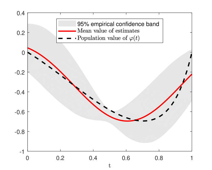
(a) $n=1000,J_{0}=\infty$

(b) $n=5000,J_{0}=\infty$

(c) $n=1000,J_{0}=2$

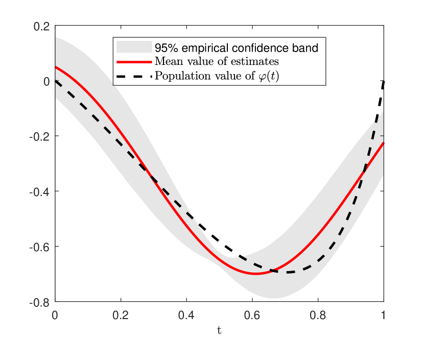
(d) $n=5000,J_{0}=2$

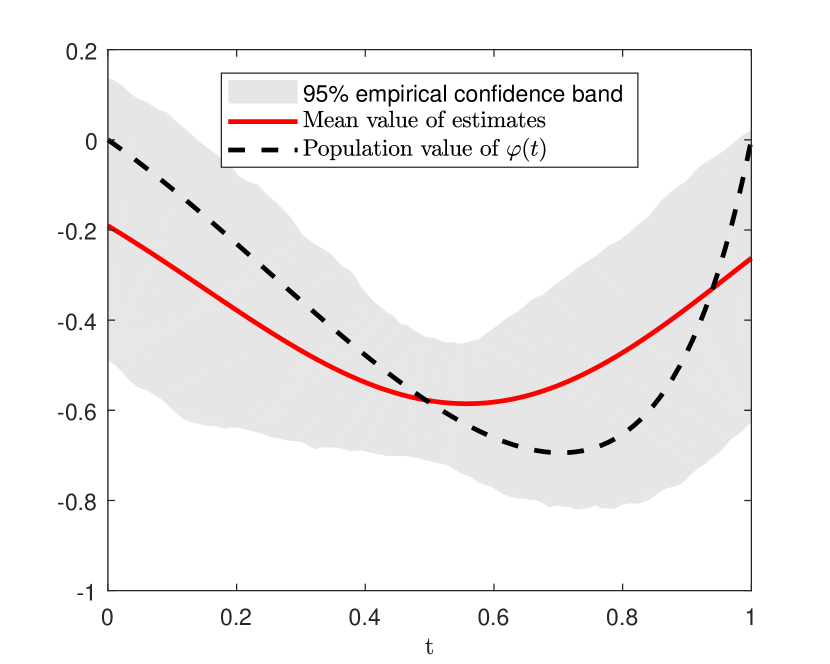
(e) $n=1000,J_{0}=1$

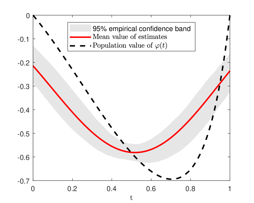
(f) $n=5000,J_{0}=1$

Figure 1: Estimates averaged over $5000$ experiments with 95% pointwise empirical confidence bands.

7 Conclusion

This paper develops a theory of nonidentified ill-posed inverse problems using the nonparametric IV and the high-dimensional regressions as illustrating examples. Identification failures occur due to the non-injectivity of the covariance or the conditional expectation operators. We show that if these operators are not injective, the estimators based on the spectral regularization converge to the best approximation of the structural parameter in the orthogonal complement to the null space of the operator and derive new uniform and Hilbert space norm bounds for the risk.

This provides us an appealing projection interpretation for the nonparametric IV regression under identification failures similar to the one shared by the ordinary least-squares under misspecification. We describe several circumstances when the best approximation coincides with a structural parameter, or at least reasonably approximates it, and discuss how our results can be useful in the partial identification setting under smoothness constraints. It is also worth mentioning that the smoothnes constraints can also be incorporated in the regularization procedure, see Babii and Florens (2021), leading to more precise estimates in small samples.

Lastly, we illustrate that under identification failures, the asymptotic distribution of linear functionals can transition between the weighted chi-squared and Gaussian limits.

APPENDIX

A.1 General regularization schemes

Consider a linear operator equation

$$K\varphi=r,$$

where $K:\mathcal{E}\to\mathcal{H}$ is a linear operator and $\mathcal{E},\mathcal{H}$ are Hilbert spaces. The operator $K$ is assumed to be bounded with $\|K\|^{2}\leq\Lambda$ for some $\Lambda<\infty$, but not necessarily compact. Then $K^{*}K:\mathcal{E}\to\mathcal{E}$ is a normal operator with spectral decomposition

$$K^{*}K=\int_{\sigma(K^{*}K)}\lambda\mathrm{d}E(\lambda),$$

where $\sigma(K^{*}K)$ is the spectrum of $K^{*}K$ and $E$ is the resolution of identity; see Rudin (1991), Theorem 12.23. For a bounded Borel function $g:[0,\Lambda]\to\mathbf{R}$, define

$$g(K^{*}K)=\int_{\sigma(K^{*}K)}g(\lambda)\mathrm{d}E(\lambda).$$

If additionally the operator $K$ is compact, the spectrum of $K^{*}K$ is countable, and

$$g(K^{*}K)=\sum_{j=1}^{\infty}g(\lambda_{j})E_{j},$$

where $E_{j}$ is a projection operator on the eigenspace corresponding to $\lambda_{j}$. If $(\varphi_{j},\psi_{j})_{j\geq 1}$ is a sequence of eigenvectors of $K^{*}K$, then for all $\varphi\in\mathcal{E}$

$$g(K^{*}K)\varphi=\sum_{j=1}^{\infty}g(\lambda_{j})\langle\varphi,\varphi_{j}\rangle\psi_{j}.$$

We are interested in recovering the best approximation to the structural parameter $\varphi$ when estimates $(\hat{K},\hat{r})$ of $(K,r)$ are available with $\|\hat{K}\|^{2}\leq\Lambda$ a.s. To that end, we consider a slightly more general version of Assumption 3.1:

Assumption A.1.1.

Suppose that $(\varphi,K)$ belongs to

$$\mathcal{F}(\beta,C)=\left\{(\varphi,K):\;\varphi_{1}=s_{\beta}(K^{*}K)\psi,\;\|\psi\|^{2}\vee\|\varphi_{0}\|\vee\|K\|\leq C\right\},$$

where $s_{\beta}:[0,\Lambda]\to\mathbf{R}$ is a nondecreasing positive function such that $\lambda\mapsto s_{\beta}^{2}(\lambda)/\lambda^{\beta}$ is nonincreasing.

The following two cases are of interest:

1. mildly ill-posed problem: $s_{\beta}(\lambda)=\lambda^{\beta/2}$;

2. severely ill-posed problem: $s_{\beta}(\lambda)=\log^{-\beta/2}\left(\frac{1}{\lambda}\right)$ with $s_{\beta}(0)=0$.

It is worth mentioning that the mildly ill-posed case allows for the exponential decline of eigenvalues of $K^{*}K$ provided that the Fourier coefficients of $\varphi_{1}$ also decline exponentially fast. On the other hand, the severely ill-posed case allows for less regular $\varphi_{1}$.

The spectral regularization scheme is described by the family of bounded Borel functions $g_{\alpha}:[0,\infty)\to\mathbf{R}$, where $\alpha>0$ is a regularization parameter such that $\lim_{\alpha\to 0}g_{\alpha}(\lambda)=\lambda^{-1}$. Assuming that $\hat{K}$ is bounded, the regularized estimator is defined as

$$\hat{\varphi}=g_{\alpha}(\hat{K}^{*}\hat{K})\hat{K}^{*}\hat{r}.$$

Our theoretical results require that the regularization scheme satisfies the following assumption:

Assumption A.1.2.

There exist $c_{1},c_{2},c_{3},\beta_{0}>0$ such that: (i) $\sup_{\lambda\leq\Lambda}|g_{\alpha}(\lambda)\lambda^{1/2}|\leq c_{1}/\sqrt{\alpha}$; (ii) $\sup_{\lambda\leq\Lambda}|(g_{\alpha}(\lambda)\lambda-1)\lambda^{r}|\leq c_{2}\alpha^{r},\forall r\in[0,2\beta_{0}]$; and (iii) $\sup_{\lambda\leq\Lambda}|g_{\alpha}(\lambda)|\leq c_{3}/\alpha$.

It is easy to verify that the following regularization schemes satisfy Assumption A.1.2 in the mildly and the severely ill-posed cases:

1. Tikhonov regularization:

   $$g_{\alpha}(\lambda)=\frac{1}{\alpha+\lambda}.$$

   Assumption A.1.2 holds with $c_{1}=1/2$, $c_{2}=c_{3}=1$, and $\beta_{0}=2$.

2. Spectral cut-off regularization (principal components):

   $$g_{\alpha}(\lambda)=\lambda^{-1}\mathds{1}\{\lambda\geq\alpha\}.$$

   Assumption A.1.2 holds with $c_{1}=c_{2}=c_{3}=1$ and every $\beta_{0}>0$.

3. Iterated Tikhonov regularization:

   $$g_{\alpha,m}(\lambda)=\sum_{j=0}^{m-1}\frac{\alpha^{j}}{(\alpha+\lambda)^{j+1}}=\frac{1}{\lambda}\left(1-\left(\frac{\alpha}{\lambda+\alpha}\right)^{m}\right),\qquad m=2,3,\dots$$

   Assumption A.1.2 holds with $c_{1}=m^{1/2}$, $c_{2}=1$ and $c_{3}=\beta_{0}=m$.

4. Landweber-Fridman regularization:

   $$g_{\alpha,c}(\lambda)=\sum_{j=0}^{1/\alpha-1}(1-c\lambda)^{j}=\frac{1}{\lambda}\left(1-(1-c\lambda)^{1/\alpha}\right),$$

   where $\alpha=1/m$ for some $m\in\mathbf{N}$ and $c\in(0,1/\Lambda)$. Assumption A.1.2 is satisfied with $c_{1}^{2}=c$, $c_{2}=c\vee 1$, $c_{3}=\left(\frac{\beta}{ce}\right)^{\beta/2}\vee 1$, and every $\beta_{0}>0$.

The constant $\beta_{0}$ is called the qualification of the regularization scheme. It is well known that the simple Tikhonov regularization exhibits a saturation effect and its bias cannot converge faster than at the rate $O(\alpha^{2})$. This can be fixed with the iterated Tikhonov regularization similarly to using higher-order kernels for nonparametric kernel estimators.

The following result describes the rate of convergence of $\hat{\varphi}$ to $\varphi_{1}$ for general regularization schemes:

Theorem A.1.

Suppose that Assumptions A.1.1, A.1.2, and 3.2 are satisfied with $\beta\leq\beta_{0}$. Then in the mildly ill-posed case

$$\left\|\hat{\varphi}-\varphi_{1}\right\|^{2}=O_{P}\left(\frac{\delta_{n}}{\alpha_{n}}+\rho_{1n}^{\beta\wedge 1}\left(1+\mathds{1}_{\beta=1}\log^{2}\rho_{1n}^{-1}\right)+\alpha_{n}^{\beta}\right),$$

while in the severely ill-posed case

$$\left\|\hat{\varphi}-\varphi_{1}\right\|^{2}=O_{P}\left(\frac{\delta_{n}}{\alpha_{n}}+\log^{-\beta}\rho_{1n}^{-1}+\log^{-\beta}\alpha_{n}^{-1}\right).$$

Before we state the proof, note that

1. In the mildly ill-posed case, the optimal choice of regularization parameter is $\alpha_{n}\sim\delta_{n}^{\frac{1}{\beta+1}}$ provided that $\rho_{1n}^{\beta\wedge 1}\log^{2}n\lesssim\delta_{n}/\alpha_{n}$. Then the convergence rate is

   $$\|\hat{\varphi}-\varphi_{1}\|^{2}=O_{P}\left(\delta_{n}^{\frac{\beta}{\beta+1}}\right).$$

2. In the severelly ill-posed case, one can choose $\alpha_{n}\sim\delta_{n}^{1/2}$. Then the convergence rate is

   $$\|\hat{\varphi}-\varphi_{1}\|^{2}=O_{P}\left(\frac{1}{\log^{\beta}n}\right),$$

   provided that $\delta_{n},\rho_{n}\sim n^{-c}$ for some $c>0$.

Proof of Theorem A.1.

Decompose

$$\hat{\varphi}-\varphi_{1}=I_{n}+II_{n}+III_{n}$$

with

$$I_{n} =g_{\alpha}(\hat{K}^{*}\hat{K})\hat{K}^{*}(\hat{r}-\hat{K}\varphi),$$

$$II_{n} =\left[g_{\alpha}(\hat{K}^{*}\hat{K})\hat{K}^{*}\hat{K}-I\right]s_{\beta}(\hat{K}^{*}\hat{K})\psi,$$

$$III_{n} =\left[g_{\alpha}(\hat{K}^{*}\hat{K})\hat{K}^{*}\hat{K}-I\right]\left\{s_{\beta}(K^{*}K)-s_{\beta}(\hat{K}^{*}\hat{K})\right\}\psi.$$

To see that this decomposition holds, note that $\varphi=\varphi_{1}+\varphi_{0}$ and that under Assumption A.1.1, $\varphi_{1}=s_{\beta}(K^{*}K)\psi$. By the isometry of functional calculus

$$\|I_{n}\|^{2} \leq\left\|g_{\alpha}(\hat{K}^{*}\hat{K})\hat{K}^{*}\right\|^{2}\left\|\hat{r}-\hat{K}\varphi_{1}\right\|^{2}$$

$$\leq\sup_{\lambda\leq\Lambda}\left|g_{\alpha}(\lambda)\lambda^{1/2}\right|^{2}\left\|\hat{r}-\hat{K}\varphi_{1}\right\|^{2},$$

which under Assumptions A.1.2 (i) and 3.2 shows that $\mathds{E}\|I_{n}\|^{2}=O\left(\delta_{n}/\alpha_{n}\right)$.

Next

$$\|II_{n}\|^{2} \leq\left\|\left[g_{\alpha}(\hat{K}^{*}\hat{K})\hat{K}^{*}\hat{K}-I\right]s_{\beta}(\hat{K}^{*}\hat{K})\right\|^{2}\left\|\psi\right\|^{2}$$

$$\leq\sup_{\lambda\leq\Lambda}\left|(g_{\alpha}(\lambda)\lambda-1)s_{\beta}(\lambda)\right|^{2}C$$

Under Assumption A.1.1, $s_{\beta}$ is nondecreasing, whence under Assumption A.1.2 (ii) with $r=0$, we obtain

$$\left|(g_{\alpha}(\lambda)\lambda-1)s_{\beta}(\lambda)\right|\leq c_{2}|s_{\beta}(\lambda)|\leq c_{2}s_{\beta}(\alpha_{n}),\qquad\forall\lambda\in[0,\alpha_{n}].$$

Similarly, since $\lambda\mapsto s_{\beta}(\lambda)/\lambda^{\beta/2}$ is nonincreasing, under Assumption A.1.2 (ii) with $r=\beta/2$

$$\left|(g_{\alpha}(\lambda)\lambda-1)s_{\beta}(\lambda)\right|\leq\left|(g_{\alpha}(\lambda)\lambda-1)\lambda^{\beta/2}\right|\left|\frac{s_{\beta}(\lambda)}{\lambda^{\beta/2}}\right|\leq c_{2}\alpha_{n}^{\beta/2}s_{\beta}(\alpha_{n})/\alpha_{n}^{\beta/2},\qquad\forall\lambda\geq\alpha_{n}.$$

Therefore, $\|II_{n}\|^{2}\leq Cc_{2}^{2}s_{\beta}^{2}(\alpha_{n})$.

Lastly, under Assumption A.1.2 (ii) with $r=0$

$$\|III_{n}\|^{2} \leq\left\|g_{\alpha}(\hat{K}^{*}\hat{K})\hat{K}^{*}\hat{K}-I\right\|^{2}\left\|s_{\beta}(\hat{K}^{*}\hat{K})-s_{\beta}(K^{*}K)\right\|^{2}\left\|\psi\right\|^{2}$$

$$\leq C\sup_{\lambda\leq\Lambda}\left|(g_{\alpha}(\lambda)\lambda-1)\right|^{2}\left\|s_{\beta}(\hat{K}^{*}\hat{K})-s_{\beta}(K^{*}K)\right\|^{2}$$

$$\leq Cc_{2}^{2}\left\|s_{\beta}(\hat{K}^{*}\hat{K})-s_{\beta}(K^{*}K)\right\|^{2}.$$

The result follows by Lemma A.1.1 appearing at the end of the section. ∎

The following result provides the uniform convergence rates for a generic class of regularized estimators:

Theorem A.2.

Suppose that Assumptions A.1.1, A.1.2, 3.2, and 3.3 are satisfied with $\varphi_{1}=s_{\beta}(K^{*}K)K^{*}\psi$ and $\beta_{0}\geq\beta$. Then in the mildly ill-posed case

$$\left\|\hat{\varphi}-\varphi_{1}\right\|_{\infty}=O_{P}\left(\frac{\delta_{n}^{1/2}}{\alpha_{n}}+\frac{1}{\alpha_{n}^{1/2}}\left(\rho_{2n}^{1/2}+\rho_{1n}^{\frac{\beta\wedge 1}{2}}\left(1+\mathds{1}_{\beta=1}\log\rho_{1n}^{-1}\right)\right)+\alpha_{n}^{\beta/2}\right),$$

while in the severely ill-posed case

$$\left\|\hat{\varphi}-\varphi_{1}\right\|_{\infty}=O_{P}\left(\frac{\delta_{n}^{1/2}}{\alpha_{n}}+\frac{1}{\alpha_{n}^{1/2}}\left(\rho_{2n}^{1/2}+\log^{-\beta/2}\rho_{1n}^{-1}\right)+\log^{-\beta/2}\alpha_{n}^{-1}\right).$$

Proof.

Consider the following decomposition

$$\hat{\varphi}-\varphi_{1}=I_{n}+II_{n}+III_{n}$$

with

$$I_{n} =g_{\alpha}(\hat{K}^{*}\hat{K})\hat{K}^{*}(\hat{r}-\hat{K}\varphi_{1}),$$

$$II_{n} =\left[g_{\alpha}(\hat{K}^{*}\hat{K})\hat{K}^{*}\hat{K}-I\right]s_{\beta}(\hat{K}^{*}\hat{K})\hat{K}^{*}\psi,$$

$$III_{n} =\left[g_{\alpha}(\hat{K}^{*}\hat{K})\hat{K}^{*}\hat{K}-I\right]\left\{s_{\beta}(K^{*}K)K^{*}-s_{\beta}(\hat{K}^{*}\hat{K})\hat{K}^{*}\right\}\psi.$$

We bound the first term as

$$\|I_{n}\|_{\infty} =\left\|\hat{K}^{*}g_{\alpha}(\hat{K}\hat{K}^{*})(\hat{r}-\hat{K}\varphi_{1})\right\|$$

$$\leq\|\hat{K}^{*}\|_{2,\infty}\sup_{\lambda\leq\Lambda}|g_{\alpha}(\lambda)|\left\|\hat{r}-\hat{K}\varphi_{1}\right\|$$

$$=O_{P}\left(\frac{\delta_{n}^{1/2}}{\alpha_{n}}\right),$$

where the last line follows under Assumptions 3.3 and A.1.2 (iii).

For the second term, note that

$$\|II_{n}\|_{\infty} =\left\|\hat{K}^{*}\left[g_{\alpha}(\hat{K}\hat{K}^{*})\hat{K}\hat{K}^{*}-I\right]s_{\beta}(\hat{K}\hat{K}^{*})\psi\right\|$$

$$\leq\|\hat{K}^{*}\|_{2,\infty}\sup_{\lambda\leq\Lambda}|(g_{\alpha}(\lambda)\lambda-1)s_{\beta}(\lambda)|\|\psi\|$$

$$=O_{P}(s_{\beta}(\alpha_{n})),$$

where the last line follows by the same argument as in the proof of Theorem A.1 under Assumptions 3.3 and A.1.2 (ii).

Next, for the third term,

$$\|III_{n}\|_{\infty}\leq\left\|g_{\alpha}(\hat{K}^{*}\hat{K})\hat{K}^{*}\hat{K}-I\right\|_{\infty}\left\|s_{\beta}(K^{*}K)K^{*}-s_{\beta}(\hat{K}^{*}\hat{K})\hat{K}^{*}\right\|_{2,\infty}\|\psi\|.$$

Under Assumptions A.1.2 (i) and 3.3

$$\left\|g_{\alpha}(\hat{K}^{*}\hat{K})\hat{K}^{*}\hat{K}-I\right\|_{\infty} \leq\|\hat{K}^{*}\|_{2,\infty}\left\|g_{\alpha}(\hat{K}\hat{K}^{*})\hat{K}\right\|+1$$

$$\leq\|\hat{K}^{*}\|_{2,\infty}\sup_{\lambda\leq\Lambda}\left|g_{\alpha}(\lambda)\lambda^{1/2}\right|+1$$

$$=O_{P}\left(\frac{1}{\alpha_{n}^{1/2}}\right).$$

Lastly, under Assumption 3.3

$$\left\|s_{\beta}(K^{*}K)K^{*}-s_{\beta}(\hat{K}^{*}\hat{K})\hat{K}^{*}\right\|_{2,\infty} =\left\|K^{*}s_{\beta}(KK^{*})-\hat{K}^{*}s_{\beta}(\hat{K}\hat{K}^{*})\right\|_{2,\infty}$$

$$\lesssim\left\|\hat{K}^{*}-K^{*}\right\|_{2,\infty}+\left\|s_{\beta}(\hat{K}^{*}\hat{K})-s_{\beta}(K^{*}K)\right\|$$

$$\lesssim\rho_{2n}^{1/2}+\left\|s_{\beta}(\hat{K}^{*}\hat{K})-s_{\beta}(K^{*}K)\right\|$$

The result now follows by Lemma A.1.1 as in the proof of Theorem A.1. ∎

Lemma A.1.1.

Suppose that Assumption 3.2 (iii) is satisfied with $\rho_{1n}\sim n^{-c}$ for some $c>0$. Then

$$\left\|(\hat{K}^{*}\hat{K})^{\beta/2}-(K^{*}K)^{\beta/2}\right\|=O_{P}\left(\left(1+\mathds{1}_{\beta=1}\log\rho_{1n}^{-1}\right)\rho_{1n}^{\frac{\beta\wedge 1}{2}}\right)$$

and

$$\left\|\log^{-\beta/2}(\hat{K}^{*}\hat{K})^{-1}-\log^{-\beta/2}(K^{*}K)^{-1}\right\|=O_{P}\left(\log^{-\beta/2}\rho_{1n}^{-1}\right).$$

Proof.

By Egger (2005), Lemma 3.2,

$$\left\|(\hat{K}^{*}\hat{K})^{\beta/2}-(K^{*}K)^{\beta/2}\right\|\lesssim\begin{cases}\|\hat{K}-K\|^{\beta},&\beta<1\\ \|\hat{K}-K\|\left\{1+\|\hat{K}\|+\|K\|+\log\|\hat{K}-K\|^{-1}\right\},&\beta=1\\ \|\hat{K}-K\|(\|\hat{K}\|+\|K\|)^{\beta/2},&\beta>1.\end{cases}$$

Then the first statement follows since $\|\hat{K}-K\|=O_{P}(\rho_{1n}^{1/2})$ with $\rho_{1n}\to 0$ as $n\to\infty$ under Assumption 3.2 (iii) and since $x\mapsto x\log(1/x)$ is strictly increasing in the neighborhood of zero.

For the second statement, by Mathé and Pereverzev (2002), Theorem 4

$$\left\|\log^{-\beta/2}(\hat{K}^{*}\hat{K})^{-1}-\log^{-\beta/2}(K^{*}K)^{-1}\right\| =O_{P}\left(\log^{-\beta/2}\|\hat{K}^{*}\hat{K}-K^{*}K\|^{-1}\right)$$

$$=O_{P}\left(\log^{-\beta/2}\rho_{1n}^{-1}\right),$$

where the second line follows under Assumption 3.2 (iii) and since $x\mapsto\log^{-\beta/2}(1/x)$ is strictly increasing in the neighborhood of zero. ∎

A.2 Extreme nonidentification

In this section, we obtain an approximation of the large sample distribution of the Tikhonov-regularized estimators in extremely nonidentified cases. Interestingly, we show that the asymptotic distribution is a weighted sum of independent chi-squared random variables. This result will serve as a starting point for Section 5, where we document a certain transition between the chi-squared and the Gaussian limits in the intermediate cases.

A.2.1 High-dimensional regressions

In the high-dimensional regressions, the identification strength is described by the covariance operator of $Z$ and $W$. In the extremely nonidentified case, the covariance operator is degenerate and we obtain the following result.

Theorem A.1.

Suppose that Assumption 5.1 is satisfied, $\mathds{E}[\langle Z,\delta\rangle W]=0,\;\forall\delta\in\mathcal{E}$, and $\alpha_{n}n\to\infty$. Then

$$\alpha_{n}n(\hat{\varphi}-\varphi_{1})\xrightarrow{d}\mathds{E}\left[\|W\|^{2}YZ\right]+J(h),$$

where $h(X,X^{\prime})=\frac{1}{2}\langle W,W^{\prime}\rangle(ZY^{\prime}+Z^{\prime}Y)$, $X^{\prime}=(Y^{\prime},Z^{\prime},W^{\prime})$ is an independent copy of $X=(Y,Z,W)$, and $J$ is a stochastic Wiener-Itô integral.

Note that the theorem states the weak convergence in the topology of the Hilbert space $\mathcal{E}$, which is impossible to achieve in the regular identified case. It can be shown that the distribution of inner products of $J(h)$ with $\mu\in\mathcal{E}$ is a weighted sum of chi-squared random variables. Also, interestingly, Theorem A.1 does not require that $\alpha_{n}\to 0$ as $n\to\infty$.

A.2.2 Nonparametric IV regression

In the nonparametric IV regression, the identification strength is described by the conditional expectation operator. In the extreme non-identified case,

$$\mathds{E}[\phi(Z)|W]=0,\qquad\forall\phi\in L_{2,0}(Z),$$

where $L_{2,0}(Z)=\left\{\phi\in L_{2}(Z):\;\mathds{E}\phi(Z)=0\right\}$, so that $K$ is a degenerate conditional expectation operator. Consider the operator $T:\phi\mapsto\mathds{E}_{X}[\phi(X)h(X,X^{\prime})]$ on $L_{2}(X)$, where $\mathds{E}_{X}$ is expectation with respect to $X=(Y,Z,W)$ only, $X^{\prime}$ is an independent copy of $X$, and

$$h(x,x^{\prime})=\frac{1}{2}\left\{yP_{0}\mu(z^{\prime})+y^{\prime}P_{0}\mu(z)\right\}h_{w}^{-q}\bar{K}\left(h_{w}^{-1}(w-w^{\prime})\right).$$

Here and later, $P_{0}$ is the projection operator on $L_{2,0}$ and $\bar{K}(v)=\int K_{w}(v-u)K_{w}(u)\mathrm{d}u$ is the convolution kernel. The following assumption is a set of mild restrictions on the distribution of the data:

Assumption A.2.1.

(i) $(Y_{i},Z_{i},W_{i})_{i=1}^{n}$ is an i.i.d. sample of $(Y,Z,W)$; (ii) $\mathds{E}\left[|Y||Z\right]<\infty$, $\mathds{E}[|Y|^{2}|W]<\infty$ a.s.; (iii) $K_{j}\in L_{1}\cap L_{2},j\in\{z,w\}$ and $K_{w}$ is a symmetric and bounded function; (iv) $f_{Z}\in L_{\infty}$.

Let $h_{z}$ and $h_{w}$ be the bandwidth parameters smoothing respectively over $Z$ and $W$. The following result holds:

Theorem A.2.

Suppose that Assumption A.2.1 is satisfied, $\mathds{E}[\phi(Z)|W]=0,\forall\phi\in L_{2,0}(Z)$, and $n\alpha_{n}h_{z}^{p}\to\infty$ with $h_{w}$ being fixed. Then for every $\mu\in L_{2}([0,1]^{p})$

$$\alpha_{n}n\langle\hat{\varphi}-\varphi_{1},\mu\rangle\xrightarrow{d}\mathds{E}\left[YP_{0}\mu(Z)\right]h_{w}^{-q}\bar{K}(0)+\sum_{j=1}^{\infty}\lambda_{j}(\chi_{j}^{2}-1),$$

where $(\chi^{2}_{j})_{j\geq 1}$ are independent chi-squared random variables with 1 degree of freedom and $(\lambda_{j})_{j\geq 1}$ are eigenvalues of $T$.

It is worth mentioning that obtaining the functional convergence of $\alpha_{n}n(\hat{\varphi}-\varphi_{1})$ is impossible in the case of the nonparametric IV regression. Note that when $h_{w}\to 0$, then with a suitable normalization we can obtain only convergence to a fixed constant.

A.3 Proofs of main results

Proof of Theorem 3.1.

Decompose

$$\hat{\varphi}-\varphi_{1} =(\alpha_{n}I+\hat{K}^{*}\hat{K})^{-1}\hat{K}^{*}(\hat{r}-\hat{K}\varphi_{1})$$

$$+(\alpha_{n}I+\hat{K}^{*}\hat{K})^{-1}\hat{K}^{*}\hat{K}\varphi_{1}-(\alpha_{n}I+K^{*}K)^{-1}K^{*}K\varphi_{1}$$

$$+\left((\alpha_{n}I+K^{*}K)^{-1}K^{*}K-I\right)\varphi_{1}$$

$$\triangleq I_{n}+II_{n}+III_{n}.$$

$III_{n}$ is the regularization bias that can controlled under Assumption 3.1

$$\|III_{n}\|^{2} =\left\|\alpha_{n}(\alpha_{n}I+K^{*}K)^{-1}\varphi_{1}\right\|^{2}$$

$$\leq C\left\|\alpha_{n}(\alpha_{n}I+K^{*}K)^{-1}(K^{*}K)^{\beta/2}\right\|^{2}$$

$$\leq C\sup_{\lambda\in[0,\|K\|^{2}]}\left|\frac{\alpha_{n}\lambda^{\beta/2}}{\alpha_{n}+\lambda}\right|^{2}$$

$$\leq C^{(2\beta-3)\vee 1}\alpha_{n}^{\beta},$$

see Babii (2021). The first term is controlled under Assumption 3.2 (i)

$$\mathds{E}\|I_{n}\|^{2} \leq\mathds{E}\left\|(\alpha_{n}I+\hat{K}^{*}\hat{K})^{-1}\hat{K}^{*}\right\|^{2}\left\|\hat{r}-\hat{K}\varphi_{1}\right\|^{2}$$

$$\leq\sup_{\lambda\geq 0}\left|\frac{\lambda^{1/2}}{\alpha_{n}+\lambda}\right|^{2}\mathds{E}\left\|\hat{r}-\hat{K}\varphi_{1}\right\|^{2}$$

$$\leq\frac{1}{4\alpha_{n}}\mathds{E}\left\|\hat{r}-\hat{K}\varphi_{1}\right\|^{2}$$

$$\leq\frac{C_{1}\delta_{n}}{4\alpha_{n}}.$$

The second term is decomposed further

$$II_{n} =-\left[\alpha_{n}(\alpha_{n}I+\hat{K}^{*}\hat{K})^{-1}-\alpha_{n}(\alpha_{n}I+K^{*}K)^{-1}\right]\varphi_{1}$$

$$=-(\alpha_{n}I+\hat{K}^{*}\hat{K})^{-1}\alpha_{n}\left[K^{*}K-\hat{K}^{*}\hat{K}\right](\alpha_{n}I+K^{*}K)^{-1}\varphi_{1}$$

$$=(\alpha_{n}I+\hat{K}^{*}\hat{K})^{-1}\hat{K}^{*}\left[\hat{K}-K\right]\alpha_{n}(\alpha_{n}I+K^{*}K)^{-1}\varphi_{1}$$

$$\qquad+(\alpha_{n}I+\hat{K}^{*}\hat{K})^{-1}\left[\hat{K}^{*}-K^{*}\right]\alpha_{n}K(\alpha_{n}I+K^{*}K)^{-1}\varphi_{1}$$

$$=II^{a}_{n}+II^{b}_{n}.$$

It follows from the previous computations and Assumption 3.2 (iii) that

$$\mathds{E}\|II^{a}_{n}\|^{2} =\mathds{E}\left\|(\alpha_{n}I+\hat{K}^{*}\hat{K})^{-1}\hat{K}^{*}\left[\hat{K}-K\right]\alpha_{n}(\alpha_{n}I+K^{*}K)^{-1}\varphi_{1}\right\|^{2}$$

$$\leq\mathds{E}\left\|(\alpha_{n}I+\hat{K}^{*}\hat{K})^{-1}\hat{K}^{*}\right\|^{2}\left\|\hat{K}-K\right\|^{2}\left\|\alpha_{n}(\alpha_{n}I+K^{*}K)^{-1}\varphi_{1}\right\|^{2}$$

$$\leq\sup_{\lambda\geq 0}\left|\frac{\lambda^{1/2}}{\alpha_{n}+\lambda}\right|^{2}\mathds{E}\left\|\hat{K}-K\right\|^{2}C^{(2\beta-3)\vee 1}\alpha_{n}^{\beta\wedge 2}$$

$$\leq\frac{C_{2}\rho_{1n}}{4\alpha_{n}}C^{(2\beta-3)\vee 1}\alpha_{n}^{\beta\wedge 2}$$

and

$$\mathds{E}\|II^{b}_{n}\|^{2} =\mathds{E}\left\|(\alpha_{n}I+\hat{K}^{*}\hat{K})^{-1}\left[\hat{K}^{*}-K^{*}\right]\alpha_{n}K(\alpha_{n}I+K^{*}K)^{-1}\varphi_{1}\right\|^{2}$$

$$\leq\mathds{E}\left\|(\alpha_{n}I+\hat{K}^{*}\hat{K})^{-1}\right\|^{2}\left\|\hat{K}^{*}-K^{*}\right\|^{2}C\left\|\alpha_{n}K(\alpha_{n}I+K^{*}K)^{-1}(K^{*}K)^{\beta/2}\right\|^{2}$$

$$\leq\sup_{\lambda\geq 0}\left|\frac{1}{\alpha_{n}+\lambda}\right|^{2}\mathds{E}\left\|\hat{K}^{*}-K^{*}\right\|^{2}C\sup_{\lambda\in[0,C^{2}]}\left|\frac{\alpha_{n}\lambda^{(\beta+1)/2}}{\alpha_{n}+\lambda}\right|^{2}$$

$$\leq\frac{C_{2}\rho_{1n}}{\alpha_{n}^{2}}C^{(2\beta-1)\vee 1}\alpha_{n}^{(\beta+1)\wedge 2},$$

where we use $\|\hat{K}^{*}-K^{*}\|=\|\hat{K}-K\|$. Combining all estimates together, we obtain the result. ∎

Proof of the Theorem 3.2.

Consider the same decomposition as in the proof of Theorem 3.1. Since $\varphi_{1}=(K^{*}K)^{\beta/2}K^{*}\psi$, the bias term is treated similarly to the identified case, see Babii (2020), Proposition 3.1

$$\|III_{n}\|_{\infty} =\left\|\alpha_{n}K^{*}(\alpha_{n}I+KK^{*})^{-1}(KK^{*})^{\frac{\beta}{2}}\psi\right\|_{\infty}$$

$$\leq\left\|K^{*}\right\|_{2,\infty}\left\|\alpha_{n}(\alpha_{n}I+KK^{*})^{-1}(KK^{*})^{\frac{\beta}{2}}\right\|\left\|\psi\right\|$$

$$=O(\alpha_{n}^{\beta/2}).$$

Next, by the Cauchy-Schwartz inequality and Assumption 3.2 (iii) and Assumption 3.3, the first term is

$$\mathds{E}\|I_{n}\|_{\infty} =\mathds{E}\left\|\hat{K}^{*}(\alpha_{n}I+\hat{K}\hat{K}^{*})^{-1}(\hat{r}-\hat{K}\varphi_{1})\right\|_{\infty}$$

$$\leq\mathds{E}\|\hat{K}^{*}\|_{2,\infty}\left\|(\alpha_{n}I+\hat{K}\hat{K}^{*})^{-1}\right\|\left\|(\hat{r}-\hat{K}\varphi_{1})\right\|$$

$$\leq\frac{1}{\alpha_{n}}\left(\|K^{*}\|_{2,\infty}\mathds{E}\left\|(\hat{r}-\hat{K}\varphi_{1})\right\|+\mathds{E}\left\|\hat{K}^{*}-K^{*}\right\|_{2,\infty}\left\|(\hat{r}-\hat{K}\varphi_{1})\right\|\right)$$

$$\leq C_{1}^{1/2}\left(C_{3}+C_{3}^{1/2}\rho_{2n}^{1/2}\right)\frac{\delta_{n}^{1/2}}{\alpha_{n}}.$$

The second term is decomposed further similarly as in the proof of Theorem 3.1 in $II_{n}^{a}$ and $II_{n}^{b}$. We bound each of the two terms separately. First,

$$\mathds{E}\|II_{n}^{a}\|_{\infty} =\left\|\hat{K}^{*}(\alpha_{n}I+\hat{K}\hat{K}^{*})^{-1}\left[\hat{K}-K\right]\alpha_{n}(\alpha_{n}I+K^{*}K)^{-1}\varphi_{1}\right\|_{\infty}$$

$$\leq\mathds{E}\left\|\hat{K}^{*}\right\|_{2,\infty}\left\|(\alpha_{n}I+\hat{K}\hat{K}^{*})^{-1}\right\|\left\|\hat{K}-K\right\|\left\|\alpha_{n}(\alpha_{n}I+K^{*}K)^{-1}\varphi_{1}\right\|$$

$$\leq\frac{1}{\alpha_{n}}\left(C_{3}+\left(\mathds{E}\left\|\hat{K}^{*}-K^{*}\right\|_{2,\infty}^{2}\right)^{1/2}\right)\left(\mathds{E}\left\|\hat{K}-K\right\|^{2}\right)^{1/2}C^{(\beta-1.5)\vee 0.5}\alpha_{n}^{\beta/2}$$

$$\leq\left(C_{3}+C_{3}^{1/2}\rho_{2n}^{1/2}\right)\frac{C_{2}^{1/2}\rho_{1n}^{1/2}}{\alpha_{n}}C^{(\beta-1.5)\vee 0.5}\alpha_{n}^{\beta/2}.$$

Second, under Assumption 3.3, by the inequality in Babii (2020), Lemma A.4.1, see also Nair (2009), Problem 5.8

$$\mathds{E}\|II_{n}^{b}\|_{\infty} =\mathds{E}\left\|(\alpha_{n}I+\hat{K}^{*}\hat{K})^{-1}\left[\hat{K}^{*}-K^{*}\right]\alpha_{n}K(\alpha_{n}I+K^{*}K)^{-1}\varphi_{1}\right\|_{\infty}$$

$$=\mathds{E}\left\|(\alpha_{n}I+\hat{K}^{*}\hat{K})^{-1}\right\|_{\infty}\left\|\hat{K}^{*}-K^{*}\right\|_{2,\infty}\left\|\alpha_{n}K(\alpha_{n}I+K^{*}K)^{-1}\varphi_{1}\right\|$$

$$=\frac{1}{2\alpha_{n}^{3/2}}\mathds{E}\left(\|\hat{K}^{*}\|_{2,\infty}+2\alpha_{n}^{1/2}\right)\left\|\hat{K}^{*}-K^{*}\right\|_{2,\infty}C^{(\beta-1/2)\vee 1/2}\alpha_{n}^{\frac{\beta+1}{2}\wedge 1}$$

$$\leq\frac{1}{2\alpha_{n}^{3/2}}\left(C_{3}+C_{3}^{1/2}\rho_{2n}^{1/2}+2\alpha_{n}^{1/2}\right)C_{3}^{1/2}\rho_{2n}^{1/2}C^{(\beta-1/2)\vee 1/2}\alpha_{n}^{\frac{\beta+1}{2}\wedge 1}.$$

Collecting all estimates together, we obtain the result. ∎

The following proposition provides low-level conditions for Assumptions 3.2 and 3.3 in the nonparametric IV regression estimated with kernel smoothing. Let $C^{s}_{M}$ denote the the Hölder class.

Proposition A.3.1.

Suppose that (i) $(Y_{i},Z_{i},W_{i})_{i=1}^{n}$ are i.i.d. and $\mathds{E}|Y_{1}|^{2}\leq C\infty$; (ii) $f_{ZW}\in C^{s}_{M}$; (iii) kernel functions $K_{z}:\mathbf{R}^{p}\to\mathbf{R}$ and $K_{w}:\mathbf{R}^{q}\to\mathbf{R}$ are such that for $l\in\{w,z\}$, $K_{l}\in L_{1}\cap L_{2}$, $\int K_{l}(u)\mathrm{d}u=1$, $\int\|u\|^{s}K_{l}(u)\mathrm{d}u<\infty$, and $\int u^{k}K_{l}(u)\mathrm{d}u=0$ for all multindices $|k|=1,\dots,\lfloor s\rfloor$. Then

$$\mathds{E}\left\|\hat{r}-\hat{K}\varphi_{1}\right\|^{2}=O\left(\frac{1}{nh^{q}_{n}}+h^{2s}_{n}\right)\qquad\mathrm{and}\qquad\mathds{E}\left\|\hat{K}-K\right\|^{2}=O\left(\frac{1}{nh^{p+q}_{n}}+h^{2s}_{n}\right),$$

where the constants do not depend on $(K,\varphi)$.

Proof.

For the first claim, note that

$$\mathds{E}\left\|\hat{r}-\hat{K}\varphi_{1}\right\|^{2}\leq 2\mathds{E}\left\|\hat{r}-r\right\|^{2}+2\mathds{E}\left\|(\hat{K}-K)\varphi_{1}\right\|^{2}.$$

Decompose

$$\mathds{E}\left\|\hat{r}-r\right\|^{2}=\mathds{E}\left\|\hat{r}-\mathds{E}\hat{r}\right\|^{2}+\left\|\mathds{E}\hat{r}-r\right\|^{2}.$$

Under the i.i.d. assumption

$$\mathds{E}\left\|\hat{r}-\mathds{E}\hat{r}\right\|^{2} =\mathds{E}\left\|\frac{1}{nh^{q}_{n}}\sum_{i=1}^{n}Y_{i}K_{w}\left(h^{-1}_{n}(W_{i}-w)\right)-\mathds{E}\left[Y_{i}h^{-q}_{n}K_{w}\left(h^{-1}_{n}(W_{i}-w)\right)\right]\right\|^{2}$$

$$=\frac{1}{n}\mathds{E}\left\|Y_{i}h^{-q}_{n}K_{w}\left(h^{-1}_{n}(W_{i}-w)\right)-\mathds{E}\left[Y_{i}h^{-q}_{n}K_{w}\left(h^{-1}_{n}(W_{i}-w)\right)\right]\right\|^{2}$$

$$\leq\frac{1}{nh^{q}_{n}}\mathds{E}|Y_{1}|^{2}\|K_{w}\|^{2}$$

$$=O\left(\frac{1}{nh^{q}_{n}}\right).$$

By the Cauchy-Schwartz inequality

$$\mathds{E}\hat{r}-r =\mathds{E}\left[\varphi(Z_{i})h^{-q}_{n}K_{w}\left(h^{-1}_{n}(W_{i}-w)\right)\right]-\int\varphi(z)f_{ZW}(z,w)\mathrm{d}z$$

$$=\int\varphi(z)\left\{[f_{ZW}\ast K_{w}](z,w)-f_{ZW}(z,w)\right\}\mathrm{d}z$$

$$\leq\|\varphi\|\left\|f_{ZW}\ast K_{w}-f_{ZW}\right\|,$$

where we put $[f_{ZW}\ast K_{w,h}](z,w)=\int f_{ZW}(z,w^{\prime})h_{n}^{-q}K_{w}\left(h_{n}^{-1}(w-w^{\prime})\right)\mathrm{d}w^{\prime}$. Since $f_{ZW}\in C^{s}_{M}$, we obtain

$$\left\|\mathds{E}\hat{r}-r\right\|=O(h^{s}),$$

see, e.g., Giné and Nickl (2016), Proposition 4.3.8. Therefore,

$$\mathds{E}\|\hat{r}-r\|^{2}=O\left(\frac{1}{nh_{n}^{q}}+h_{n}^{2s}\right).$$

Next, decompose

$$(\hat{K}\varphi_{1}-K\varphi_{1})(w) \triangleq V_{n}(w)+B_{n}(w)$$

with

$$V_{n} =\int\varphi_{1}(z)\left(\hat{f}_{ZW}(z,w)-\mathds{E}\hat{f}_{ZW}(z,w)\right)\mathrm{d}z$$

$$B_{n} =\int\varphi_{1}(z)\left(\mathds{E}\hat{f}_{ZW}(z,w)-f_{ZW}(z,w)\right)\mathrm{d}z.$$

By the Cauchy-Schwartz inequality

$$\|B_{n}\|\leq\|\varphi_{1}\|\left\|\mathds{E}\hat{f}_{ZW}-f_{ZW}\right\|,$$

where the right side is of order $O(h_{n}^{s})$ under the assumption $f_{ZW}\in C^{s}_{M}$, see Giné and Nickl (2016), p.404.

Next, note that

$$V_{n}(w)=\frac{1}{nh_{n}^{q}}\sum_{i=1}^{n}\eta_{n,i}(w).$$

with

$$\eta_{n,i}(w)=K_{w}\left(h_{n}^{-1}(W_{i}-w)\right)\left[\varphi_{1}\ast K_{z}\right](Z_{i})-\mathds{E}\left[K\left(h_{n}^{-1}(W_{i}-w)\right)\left[\varphi_{1}\ast K_{z}\right](Z_{i})\right],$$

where $\left[\varphi_{1}\ast K_{z}\right](Z_{i})=\int\varphi_{1}(z)h_{n}^{-p}K_{z}\left(h_{n}^{-1}(Z_{i}-z)\right)\mathrm{d}z$. Then

$$\mathds{E}\|V_{n}\|^{2} \leq\frac{1}{nh_{n}^{2q}}\int\int\int\left|K_{w}(h_{n}^{-1}(w^{\prime}-w))\right|^{2}\left|\left[\varphi_{1}\ast K_{z}\right](z^{\prime})\right|^{2}\mathrm{d}wf_{ZW}(z^{\prime},w^{\prime})\mathrm{d}w^{\prime}\mathrm{d}z^{\prime}$$

$$=\frac{1}{nh_{n}^{q}}\|K_{w}\|^{2}\int\left|\left[\varphi_{1}\ast K_{z}\right](z)\right|^{2}f_{Z}(z)\mathrm{d}z$$

$$=O\left(\frac{1}{nh_{n}^{q}}\right),$$

where the second line follows by change of variables, and the last by $\|f_{Z}\|_{\infty}\leq C$, and Young’s inequality. Combining all estimates together, we obtain the first claim.

The second claim follows from the inequality

$$\mathds{E}\left\|\hat{K}-K\right\|^{2}\leq\mathds{E}\left\|\hat{f}_{ZW}-f_{ZW}\right\|^{2}$$

and the standard resultson the $L_{2}$ error of the kernel density estimator, Giné and Nickl (2016), Chapter 5. ∎

Proof of Theorem 4.1.

Note that under $H_{0}$

$$\Pr(n\hat{T}>q_{1-\alpha}) =\Pr\left(\inf_{\phi\in\mathscr{F}_{\varepsilon}:\;\|\phi\|_{\infty}=1}\|\sqrt{n}\hat{K}\phi\|^{2}>q_{1-\alpha}\right)$$

$$\leq\Pr\left(\|\sqrt{n}\hat{K}\phi\|^{2}>q_{1-\alpha}\right)$$

$$=\Pr\left(\|\sqrt{n}(\hat{K}-K)\phi\|^{2}>q_{1-\alpha}\right),$$

where the last line follows since under $H_{0}$, $K\phi=0$. Since $\mathds{E}\|WZ\|^{2}<\infty$, by the Hilbert space central limit theorem, see Bosq (2000), Theorem 2.7,

$$\sqrt{n}(\hat{K}-K)\phi =\frac{1}{\sqrt{n}}\sum_{i=1}^{n}W_{i}\langle Z_{i},\phi\rangle-\mathds{E}[W_{i}\langle Z_{i},\phi\rangle]$$

$$\xrightarrow{d}\mathbb{G}_{\phi},$$

where $\mathbb{G}_{\phi}$ is a zero-mean Gaussian process with covariance operator $C_{\phi}$. Next, by the Karhunen-Loève decomposition

$$\|\mathbb{G}_{\phi}\|^{2}=\sum_{j\geq 1}\lambda_{\phi,j}\chi_{j}^{2},$$

where $(\lambda_{\phi,j})_{j\geq 1}$ are eigenvalues of $C_{\phi}$ and $(\chi^{2}_{j})_{j\geq 1}$ are i.i.d. chi-squared random variables; see Shorack and Wellner (2009), Chapter 5. Therefore, under $H_{0}$

$$\lim_{n\to\infty}\Pr(n\hat{T}>q_{1-\alpha})\leq\alpha.$$

∎

Proof of Theorem A.1.

Since $\mathds{E}[\langle Z,\delta\rangle W]=0$ for all $\delta\in\mathcal{E}$, we have $\varphi_{1}=0$. Then

$$\alpha_{n}n\left(\hat{\varphi}-\varphi_{1}\right)=\left(I+\frac{1}{\alpha_{n}}\hat{K}^{*}\hat{K}\right)^{-1}n\hat{K}^{*}\hat{r}.$$

Under Assumption 5.1

$$\mathds{E}\|\hat{K}\|^{2}=\mathds{E}\|\hat{K}-K\|^{2}\leq\mathds{E}\left\|\frac{1}{n}\sum_{i=1}^{n}Z_{i}W_{i}-\mathds{E}[ZW]\right\|^{2}=O\left(\frac{1}{n}\right).$$

Then $\|\hat{K}^{*}\hat{K}\|\leq\|\hat{K}\|^{2}=O_{P}\left(n^{-1}\right)$. Therefore, as $\alpha_{n}n\to\infty$, by the continuous mapping theorem; see van der Vaart and Wellner (2000), Theorem 1.3.6

$$\alpha_{n}n\left(\hat{\varphi}-\varphi_{1}\right)=(I+o_{P}(1))^{-1}n\hat{K}^{*}\hat{r}.$$

By Slutsky’s theorem, see van der Vaart and Wellner (2000), Example 1.4.7, it suffices to obtain the asymptotic distribution of $n\hat{K}^{*}\hat{r}$.

Note that

$$n\hat{K}^{*}\hat{r} =\frac{1}{n}\sum_{i,j=1}^{n}\left\langle W_{i},W_{j}\right\rangle Z_{i}Y_{j}$$

$$=\frac{1}{n}\sum_{i=1}^{n}\|W_{i}\|^{2}Z_{i}Y_{i}+\frac{1}{n}\sum_{i\neq j}\left\langle W_{i},W_{j}\right\rangle Z_{i}Y_{j}.$$

Under Assumption 5.1, by the Mourier law of large numbers

$$\frac{1}{n}\sum_{i=1}^{n}\|W_{i}\|^{2}Z_{i}Y_{i}\xrightarrow{a.s.}\mathds{E}\left[\|W\|^{2}ZY\right].$$

Since $\mathds{E}[\langle Z,\delta\rangle W]=0,\forall\delta\in\mathcal{E}$, the second term is a Hilbert space-valued degenerate $U$-statistics

$$n\mathbf{U}_{n} \triangleq\frac{1}{n}\sum_{i\neq j}\left\langle W_{i},W_{j}\right\rangle Z_{i}Y_{j}$$

$$=\frac{2}{n}\sum_{i<j}\frac{Z_{i}Y_{j}+Z_{j}Y_{i}}{2}\left\langle W_{i},W_{j}\right\rangle.$$

Under the Assumption 5.1, by the Borovskich CLT, see Theorem B.1

$$n\mathbf{U}_{n}\xrightarrow{d}J(h),$$

where $J(h)=\iint_{\mathcal{X}\times\mathcal{X}}h(x_{1},x_{2})\mathbb{W}(\mathrm{d}x_{1})\mathbb{W}(\mathrm{d}x_{2})$ is a stochastic Wiener-Itô integral, $\mathbb{W}$ is a Gaussian random measure on $\mathcal{X}$, $h(X,X^{\prime})=\frac{ZY^{\prime}+Z^{\prime}Y}{2}\langle W,W^{\prime}\rangle$, and $X^{\prime}=(Y^{\prime},Z^{\prime},W^{\prime})$ is an independent copy of $X=(Y,Z,W)$. ∎

Proof of Theorem A.2.

Since $\mathds{E}[\phi(Z)|W]=0,\forall\phi\in L_{2,0}(Z)$, we have $\varphi_{1}=0$. Note also that the adjoint operator to $K$ is $P_{0}K^{*}$, where $P_{0}$ is the orthogonal projection on $L_{2,0}(Z)$. Then

$$\alpha_{n}n(\hat{\varphi}-\varphi_{1})=\left(I+\frac{1}{\alpha_{n}}P_{0}\hat{K}^{*}\hat{K}\right)^{-1}nP_{0}\hat{K}^{*}\hat{r},$$

where $\hat{P}_{0}$ is the estimator of $P_{0}$. Under Assumption A.2.1 (i) since $\mathds{E}[\phi(Z)|W]=0$ for all $\phi\in L_{2,0}(Z)$

$$\mathds{E}\left\|P_{0}\hat{K}^{*}\hat{K}\right\| \leq\mathds{E}\|P_{0}\hat{K}\|^{2}\leq\mathds{E}\|P_{0}\hat{f}_{ZW}\|^{2}$$

$$=\mathds{E}\left\|\frac{1}{nh_{z}^{p}h_{w}^{q}}\sum_{i=1}^{n}P_{0}K_{z}\left(h_{z}^{-1}(Z_{i}-z)\right)K_{w}\left(h_{z}^{-1}(W_{i}-w)\right)\right\|^{2}$$

$$\leq\frac{1}{nh_{z}^{2p}h_{w}^{2q}}\mathds{E}\left\|P_{0}K_{z}\left(h_{z}^{-1}(Z_{i}-z)\right)K_{w}\left(h_{z}^{-1}(W_{i}-w)\right)\right\|^{2}$$

$$=\frac{1}{nh_{z}^{p}h_{w}^{q}}\|P_{0}K_{z}\|\|K_{w}\|=O\left(\frac{1}{nh_{z}^{p}}\right).$$

Therefore, $\frac{1}{\alpha_{n}}\left\|\hat{P}_{0}\hat{K}^{*}\hat{K}\right\|=o_{P}(1)$ as $n\alpha_{n}h_{z}^{p}\to\infty$. Then by the continuous mapping and the Slutsky’s theorems, it suffices to characterize the asymptotic distribution of

$$nP_{0}\hat{K}^{*}\hat{r}=\frac{1}{nh_{z}^{p}h_{w}^{q}}\sum_{i,j}Y_{i}P_{0}K_{z}\left(h_{z}^{-1}(Z_{j}-z)\right)\bar{K}\left(h_{w}^{-1}(W_{i}-W_{j})\right).$$

To that end, for every $\mu\in L_{2}([0,1]^{p})$

$$\left\langle nP_{0}\hat{K}^{*}\hat{r},\mu\right\rangle =\left\langle n\hat{K}^{*}\hat{r},P_{0}\mu\right\rangle$$

$$\triangleq\zeta_{n}+\mathbf{U}_{n}+R_{n}$$

with

$$\zeta_{n} =\frac{1}{n}\sum_{i=1}^{n}Y_{i}P_{0}\mu(Z_{i})h_{w}^{-q}\bar{K}(0),$$

$$\mathbf{U}_{n} =\frac{2}{n}\sum_{i<j}\frac{1}{2}\left\{Y_{i}P_{0}\mu(Z_{j})+Y_{j}P_{0}\mu(Z_{i})\right\}h_{w}^{-q}\bar{K}\left(h_{w}^{-1}(W_{i}-W_{j})\right),$$

$$R_{n} =\frac{1}{nh_{w}^{q}}\sum_{i,j=1}^{n}Y_{i}\left\{[K_{z}\ast P_{0}\mu](Z_{j})-P_{0}\mu(Z_{j})\right\}\bar{K}\left(h_{n}^{-1}(W_{i}-W_{j})\right),$$

where $[K_{z}\ast P_{0}\mu](z)=h_{n}^{-p}\int K\left(h_{z}^{-1}(z-u)\right)P_{0}\mu(u)\mathrm{d}u$. Under Assumption A.2.1, by the strong law of large numbers

$$\zeta_{n}\xrightarrow{a.s}\mathds{E}\left[YP_{0}\mu(Z)\right]h_{w}^{-q}\bar{K}(0).$$

Since $\mathds{E}[\phi(Z)|W]=0,\forall\phi\in L_{2,0}(Z)$, $\mathbf{U}_{n}$ is a centered degenerate U-statistics. By the central limit theorem for the degenerate U-statistics, see Gregory (1977),

$$\mathbf{U}_{n}=\frac{2}{n}\sum_{i<j}h(X_{i},X_{j})\xrightarrow{d}\sum_{j=1}^{\infty}\lambda_{j}(\chi^{2}_{j}-1).$$

Lastly, decompose $R_{n}=R_{1n}+R_{2n}$ with

$$R_{1n} =\frac{1}{n}\sum_{i=1}^{n}Y_{i}\left\{[K_{z}\ast P_{0}\mu](Z_{i})-P_{0}\mu(Z_{i})\right\}h_{w}^{-q}\bar{K}(0)$$

$$R_{2n} =\frac{1}{n}\sum_{i<j}Y_{i}\left\{[K_{z}\ast P_{0}\mu](Z_{j})-P_{0}\mu(Z_{j})\right\}h_{w}^{-q}\bar{K}\left(h_{w}^{-1}(W_{i}-W_{j})\right).$$

Note that

$$\mathds{E}|R_{1n}| \leq\mathds{E}\left|Y\left\{[K_{z}\ast P_{0}\mu](Z)-P_{0}\mu(Z)\right\}\right|h_{w}^{-q}\bar{K}(0)$$

$$\lesssim\int\left|[K_{z}\ast P_{0}\mu](z)-P_{0}\mu(z)\right|f_{Z}(z)\mathrm{d}z$$

$$\leq\|K_{z}\ast\mu-\mu\|^{2}\|f_{Z}\|^{2}$$

$$=o(1),$$

where the first two lines follow under Assumption A.2.1 (i)-(ii), the third by the Cauchy-Schwartz inequality and $\|P_{0}\|\leq 1$, and the last by Giné and Nickl (2016), Proposition 4.1.1. (iii). Similarly, since $\mathds{E}\left[|Y|^{2}|W\right]<\infty$ a.s. and $\bar{K}\in L_{\infty}$, by the moment inequality in Korolyuk and Borovskich (1994), Theorem 2.1.3

$$\mathds{E}|R_{2n}|^{2} \lesssim\mathds{E}\left|Y\left\{[K_{z}\ast P_{0}\mu](Z^{\prime})-P_{0}\mu(Z^{\prime})\right\}h_{w}^{-q}\bar{K}\left(h_{w}^{-1}(W-W^{\prime})\right)\right|^{2}$$

$$\lesssim\int\left|[K_{z}\ast P_{0}\mu](z)-P_{0}\mu(z)\right|f_{Z}(z)\mathrm{d}z=o(1).$$

∎

Proof of Theorem 5.1.

Put $b_{n}=\alpha_{n}(\alpha_{n}I+K^{*}K)^{-1}\varphi_{1}$ and note that $(\alpha_{n}I+\hat{K}^{*}\hat{K})^{-1}\hat{K}^{*}=\hat{K}^{*}(\alpha_{n}I+\hat{K}\hat{K}^{*})^{-1}$. Then, similarly to the proof of Theorem 3.1, decompose

$$\left\langle\hat{\varphi}-\varphi_{1},\mu_{0}\right\rangle =\left\langle\hat{K}^{*}(\alpha_{n}I+KK^{*})^{-1}(\hat{r}-\hat{K}\varphi_{1}),\mu_{0}\right\rangle$$

$$\qquad+\left\langle\hat{K}^{*}\left((\alpha_{n}I+\hat{K}\hat{K}^{*})^{-1}-(\alpha_{n}I+KK^{*})^{-1}\right)(\hat{r}-\hat{K}\varphi_{1}),\mu_{0}\right\rangle$$

$$\qquad+\left\langle(\alpha_{n}I+\hat{K}^{*}\hat{K})^{-1}\hat{K}^{*}(\hat{K}-K)b_{n},\mu_{0}\right\rangle$$

$$\qquad+\left\langle(\alpha_{n}I+\hat{K}^{*}\hat{K})^{-1}(\hat{K}^{*}-K^{*})Kb_{n},\mu_{0}\right\rangle$$

$$\qquad+\langle b_{n},\mu_{0}\rangle$$

$$\triangleq I_{n}+II_{n}+III_{n}+IV_{n}+V_{n}.$$

Since

$$I_{n}=\left\langle\alpha_{n}(\alpha_{n}I+KK^{*})^{-1}(\hat{r}-\hat{K}\varphi_{1}),\hat{K}\mu_{0}\right\rangle,$$

it remains to show that all other terms are asymptotically negligible. Note that since $\mu_{0}\in\mathcal{N}(K)$,

$$(\alpha_{n}I+K^{*}K)^{-1}\mu_{0}=\frac{1}{\alpha_{n}}\mu_{0}.$$ (A.1)

Then

$$II_{n} =\left\langle(\alpha_{n}I+\hat{K}\hat{K}^{*})^{-1}(KK^{*}-\hat{K}\hat{K}^{*})(\alpha_{n}I+KK^{*})^{-1}(\hat{r}-\hat{K}\varphi_{1}),\hat{K}\mu_{0}\right\rangle$$

$$=\left\langle(\alpha_{n}I+\hat{K}\hat{K}^{*})^{-1}\hat{K}(K^{*}-\hat{K}^{*})(\alpha_{n}I+KK^{*})^{-1}(\hat{r}-\hat{K}\varphi_{1}),\hat{K}\mu_{0}\right\rangle$$

$$\qquad+\left\langle(\alpha_{n}I+\hat{K}\hat{K}^{*})^{-1}(K-\hat{K})K^{*}(\alpha_{n}I+KK^{*})^{-1}(\hat{r}-\hat{K}\varphi_{1}),\hat{K}\mu_{0}\right\rangle.$$

By the Cauchy-Schwartz inequality and computations similar to those in the proof of Theorem 3.1

$$II_{n} \leq\left\|(\alpha_{n}I+\hat{K}\hat{K}^{*})^{-1}\hat{K}\right\|\left\|K^{*}-\hat{K}^{*}\right\|\left\|(\alpha_{n}I+KK^{*})^{-1}\right\|\left\|\hat{r}-\hat{K}\varphi_{1}\right\|\left\|\hat{K}\mu_{0}\right\|$$

$$\quad+\left\|(\alpha_{n}I+\hat{K}\hat{K}^{*})^{-1}\right\|\left\|K-\hat{K}\right\|\left\|K^{*}(\alpha_{n}I+KK^{*})^{-1}\right\|\left\|\hat{r}-\hat{K}\varphi_{1}\right\|\left\|(\hat{K}-K)\mu_{0}\right\|$$

$$\leq\frac{1}{\alpha_{n}^{3/2}}\left\|\hat{K}-K\right\|^{2}\left\|\hat{r}-\hat{K}\varphi_{1}\right\|\|\mu_{0}\|.$$

Next, under Assumption 3.1 from the proof of Theorem 3.1 we also know that $\|b_{n}\|=O\left(\alpha_{n}^{\frac{\beta}{2}\wedge 1}\right)$ and that $\|Kb_{n}\|=O\left(\alpha_{n}^{\frac{\beta+1}{2}\wedge 1}\right)$. Therefore

$$III_{n} \leq\left\|(\alpha_{n}I+\hat{K}^{*}\hat{K})^{-1}\hat{K}^{*}\right\|\left\|\hat{K}-K\right\|\|b_{n}\|\|\mu_{0}\|$$

$$\lesssim\frac{1}{\alpha_{n}^{1/2}}\left\|\hat{K}-K\right\|\alpha_{n}^{\frac{\beta}{2}\wedge 1}.$$

and

$$IV_{n} \leq\left\|(\alpha_{n}I+\hat{K}^{*}\hat{K})^{-1}\right\|\left\|\hat{K}^{*}-K^{*}\right\|\|Kb_{n}\|\|\mu_{0}\|$$

$$\lesssim\frac{1}{\alpha_{n}^{1/2}}\left\|\hat{K}-K\right\|\alpha_{n}^{\frac{\beta\wedge 1}{2}}.$$

Lastly, the bias is zero by Eq. A.1 and the orthogonality between $\varphi_{1}$ and $\mu_{0}$

$$\langle b_{n},\mu_{0}\rangle=\left\langle\varphi_{1},\alpha_{n}(\alpha_{n}I+K^{*}K)^{-1}\mu_{0}\right\rangle=\langle\varphi_{1},\mu_{0}\rangle=0.$$

It follows from the discussion in Section 3 that under Assumption 5.1

$$\left\|\hat{K}-K\right\|=O_{P}\left(\frac{1}{n^{1/2}}\right)\quad\text{and}\quad\left\|\hat{r}-\hat{K}\varphi_{1}\right\|=O_{P}\left(\frac{1}{n^{1/2}}\right).$$

Therefore, since under Assumption 5.2 $n\alpha_{n}^{1+\beta\wedge 1}\to 0$ and $n\alpha_{n}\to\infty$,

$$n\alpha_{n}\langle\hat{\varphi}-\varphi_{1},\mu_{0}\rangle =n\alpha_{n}\left\langle(\alpha_{n}I+KK^{*})^{-1}(\hat{r}-\hat{K}\varphi_{1}),\hat{K}\mu_{0}\right\rangle+o_{P}(1)$$

$$\triangleq S_{n}+o_{P}(1)$$

with

$$S_{n}=n\alpha_{n}\left\langle(\alpha_{n}I+KK^{*})^{-1}(\hat{r}-\hat{K}\varphi_{1}),\hat{K}\mu_{0}\right\rangle.$$

Next, decompose $S_{n}=S_{n}^{0}+S_{n}^{1}$ with

$$S_{n}^{0} =\frac{1}{n}\sum_{i,j=1}^{n}(Y_{i}-\langle Z_{i},\varphi_{1}))\left\langle Z_{j},\mu_{0}\right\rangle\left\langle\alpha_{n}(\alpha_{n}I+KK^{*})^{-1}W_{i}^{0},W_{j}^{0}\right\rangle$$

$$S_{n}^{1} =\frac{1}{n}\sum_{i,j=1}^{n}(Y_{i}-\langle Z_{i},\varphi_{1}\rangle)\langle Z_{j},\mu_{0}\rangle\left\langle\alpha_{n}(\alpha_{n}I+KK^{*})^{-1}W_{i}^{1},W_{j}^{1}\right\rangle.$$

Since $W_{i}^{0}\in\mathcal{N}(K^{*})$, we have $(\alpha_{n}I+KK^{*})^{-1}W_{i}^{0}=\frac{1}{\alpha_{n}}W_{i}^{0}$. Using this fact, decompose further $S_{n}^{0}\triangleq\zeta_{n}^{0}+\mathbf{U}_{n}^{0}$ with

$$\zeta_{n}^{0} =\frac{1}{n}\sum_{i=1}^{n}(Y_{i}-\langle Z_{i},\varphi_{1}\rangle)\langle Z_{i},\mu_{0}\rangle\left\|W_{i}^{0}\right\|^{2}$$

$$\mathbf{U}_{n}^{0} =\frac{1}{n}\sum_{i<j}\left\{\langle Z_{i},\mu_{0}\rangle(Y_{j}-\langle Z_{j},\varphi_{0}\rangle)+\langle Z_{j},\mu_{0}\rangle(Y_{i}-\langle Z_{i},\mu_{0}\rangle)\right\}\left\langle W_{i}^{0},W_{j}^{0}\right\rangle.$$

Under Assumption 5.1 by the strong law of large numbers

$$\zeta_{n}^{0}\xrightarrow{a.s.}\mathds{E}\left[\left\|W^{0}\right\|^{2}(Y-\langle Z,\varphi_{1}\rangle)\langle Z,\mu_{0}\rangle\right].$$

Next, note that $W^{0}=P_{0}W$ and $W^{1}=(I-P_{0})W$, where $P_{0}$ is the projection operator on $\mathcal{N}(K^{*})$. Since projection is a bounded linear operator, it commutes with the expectation, cf., Bosq (2000), p.29, whence $\mathds{E}\left[W^{0}\langle Z,\mu_{0}\rangle\right]=P_{0}K\mu_{0}=0$ and $\mathds{E}\left[W^{0}(Y-\langle Z,\varphi_{1}\rangle)\right]=P_{0}\mathds{E}[WU]+P_{0}K\varphi_{0}=0$. Therefore, $\mathbf{U}_{n}^{0}$ is a centered degenerate $U$-statistics with a kernel function $h$. Under Assumption 5.1 by the CLT for the degenerate $U$-statistics, see Gregory (1977),

$$\mathbf{U}_{n}^{0}\xrightarrow{d}\sum_{j=1}^{\infty}\lambda_{j}(\chi_{j}^{2}-1).$$

It remains to show that $S_{n}^{1}=o_{P}(1)$. To that end decompose $S_{n}^{1}=\zeta_{n}^{1}+\mathbf{U}_{n}^{1}$ with

$$\zeta_{n}^{1} =\frac{1}{n}\sum_{i=1}^{n}(Y_{i}-\langle Z_{i},\varphi_{1}\rangle)\langle Z_{i},\mu_{0}\rangle\left\langle\alpha_{n}(\alpha_{n}I+KK^{*})^{-1}W_{i}^{1},W_{i}^{1}\right\rangle$$

$$\mathbf{U}_{n}^{1} =\frac{1}{n}\sum_{i\neq j}(Y_{i}-\langle Z_{i},\varphi_{1}\rangle)\langle Z_{j},\mu_{0}\rangle\left\langle\alpha_{n}(\alpha_{n}I+KK^{*})^{-1}W_{i}^{1},W_{j}^{1}\right\rangle.$$

It follows from Bakushinskii (1967) that $\left\|\alpha_{n}(\alpha_{n}I+KK^{*})^{-1}W^{1}\right\|=o(1)$. Then under Assumption 5.1 by the dominated convergence theorem

$$\mathds{E}\left|\zeta_{n}^{1}\right| \leq\|\mu_{0}\|\mathds{E}\left[\left(|U|+\|Z\|\|\varphi_{0}\|\right)\|Z\|\left\|\alpha_{n}(\alpha_{n}I+KK^{*})^{-1}W^{1}\right\|\right]$$

$$\lesssim\mathds{E}\left[(\|UZ\|+\|Z\|^{2})\|W\|\left\|\alpha_{n}(\alpha_{n}I+KK^{*})^{-1}W^{1}\right\|\right]$$

$$=o(1),$$

whence by Markov’s inequality $\zeta_{n}^{1}=o_{P}(1)$. Lastly, note that

$$\mathbf{U}_{n}^{1}=\frac{1}{n}\sum_{i<j} \left\{(Y_{i}-\langle Z_{i},\varphi_{1}\rangle)\langle Z_{j},\mu_{0}\rangle\left\langle\alpha_{n}(\alpha_{n}I+KK^{*})^{-1}W_{i}^{1},W_{j}^{1}\right\rangle\right.$$

$$\left.+(Y_{j}-\langle Z_{j},\varphi_{1}\rangle)\langle Z_{i},\mu_{0}\rangle\left\langle\alpha_{n}(\alpha_{n}I+KK^{*})^{-1}W_{j}^{1},W_{i}^{1}\right\rangle\right\}$$

is a centered degenerate U-statistics. Then by the moment inequality in Korolyuk and Borovskich (1994), Theorem 2.1.3,

$$\mathds{E}\left|\mathbf{U}_{n}^{1}\right|^{2} \leq 2^{-1}\mathds{E}\left|(U_{1}+\langle Z_{1},\varphi_{0}\rangle)\langle Z_{2},\mu_{0}\rangle\left\langle\alpha_{n}(\alpha_{n}I+KK^{*})^{-1}W_{1}^{1},W_{2}^{1}\right\rangle\right|^{2}$$

$$\quad+2^{-1}\mathds{E}\left|(U_{2}+\langle Z_{2},\varphi_{0}\rangle)\langle Z_{1},\mu_{0}\rangle\left\langle\alpha_{n}(\alpha_{n}I+KK^{*})^{-1}W_{2}^{1},W_{1}^{1}\right\rangle\right|^{2}$$

$$\lesssim\mathds{E}\left[\|Z\|^{2}\left\|\alpha_{n}(\alpha_{n}I+KK^{*})^{-1}W^{1}\right\|^{2}\right]=o(1),$$

where the last line follows under Assumptions 5.1 and 5.2, and previous discussions. Finally, if $W^{0}$ degenerates to zero, then $S_{n}^{0}=0$ and

$$\alpha_{n}n\langle\hat{\varphi}-\varphi_{1},\mu_{0}\rangle\xrightarrow{d}0.$$

∎

Proof of Theorem 5.2.

Similarly to the proof of Theorem 5.1, decompose

$$\left\langle\hat{\varphi}-\varphi_{1},\mu_{1}\right\rangle =\left\langle(\alpha_{n}I+K^{*}K)^{-1}K^{*}(\hat{r}-\hat{K}\varphi_{1}),\mu_{1}\right\rangle$$

$$\qquad+\left\langle\left\{(\alpha_{n}I+\hat{K}^{*}\hat{K})^{-1}-(\alpha_{n}I+K^{*}K)^{-1}\right\}\hat{K}^{*}(\hat{r}-\hat{K}\varphi_{1}),\mu_{1}\right\rangle$$

$$\qquad+\left\langle(\alpha_{n}I+K^{*}K)^{-1}(\hat{K}^{*}-K^{*})(\hat{r}-\hat{K}\varphi_{1}),\mu_{1}\right\rangle$$

$$\qquad+\left\langle(\alpha_{n}I+\hat{K}^{*}\hat{K})^{-1}\hat{K}^{*}\hat{K}\varphi_{1}-(\alpha_{n}I+K^{*}K)^{-1}K^{*}K\varphi_{1},\mu_{1}\right\rangle$$

$$\qquad+\langle b_{n},\mu_{1}\rangle$$

$$\triangleq I_{n}+II_{n}+III_{n}+IV_{n}+\langle b_{n},\mu_{1}\rangle.$$

Under Assumption 5.3 by the Lindeberg-Feller central limit theorem

$$\pi_{n}I_{n} =\frac{\pi_{n}}{n}\sum_{i=1}^{n}(U_{i}+\langle Z_{i},\varphi_{0}\rangle)\left\langle(\alpha_{n}I+K^{*}K)^{-1}K^{*}W_{i},\mu_{1}\right\rangle$$

$$\xrightarrow{d}N(0,1).$$

It remains to show that all other terms normalized with $\pi_{n}$ tend to zero. For $II_{n}$, by the Cauchy-Schwartz inequality

$$II_{n} =\left\langle\frac{1}{n}\sum_{i=1}^{n}W_{i}(U_{i}+\langle Z_{i},\varphi_{0}\rangle),\hat{K}^{*}\left((\alpha_{n}I+\hat{K}^{*}\hat{K})^{-1}-(\alpha_{n}I+K^{*}K)^{-1}\right)\mu_{1}\right\rangle$$

$$\leq\left\|\frac{1}{n}\sum_{i=1}^{n}W_{i}(U_{i}+\langle Z_{i},\varphi_{0}\rangle)\right\|\left\|\hat{K}^{*}(\alpha_{n}I+\hat{K}^{*}\hat{K})^{-1}(\hat{K}^{*}\hat{K}-K^{*}K)(\alpha_{n}I+K^{*}K)^{-1}\mu_{1}\right\|.$$

Since $\mu_{1}\in\mathcal{R}\left[(K^{*}K)^{\gamma}\right]$, there exists some $\psi\in\mathcal{E}$ such that $\mu_{1}=(K^{*}K)^{\gamma}\psi$ and so

$$II_{n} \lesssim_{P}n^{-1/2}\left\|\hat{K}^{*}(\alpha_{n}I+\hat{K}^{*}\hat{K})^{-1}\hat{K}^{*}\right\|\left\|\hat{K}-K\right\|\left\|(\alpha_{n}I+K^{*}K)^{-1}(K^{*}K)^{\gamma}\psi\right\|$$

$$\quad+n^{-1/2}\left\|\hat{K}^{*}(\alpha_{n}I+\hat{K}^{*}\hat{K})^{-1}\right\|\left\|\hat{K}^{*}-K^{*}\right\|\left\|K(\alpha_{n}I+K^{*}K)^{-1}(K^{*}K)^{\gamma}\psi\right\|$$

$$\lesssim_{P}n^{-1}\left\|(\alpha_{n}I+K^{*}K)^{-1}(K^{*}K)^{\gamma}\psi\right\|+n^{-1}\alpha_{n}^{-1/2}\left\|K(\alpha_{n}I+K^{*}K)^{-1}(K^{*}K)^{\gamma}\psi\right\|$$

$$\lesssim_{P}n^{-1}\alpha_{n}^{\gamma\wedge 1-1}+n^{-1}\alpha_{n}^{\gamma\wedge 1/2-1}=o_{P}(\pi_{n}^{-1}),$$

where the last line follows under Assumption 5.4. Similarly,

$$III_{n} \leq\left\|\hat{K}^{*}-K^{*}\right\|\left\|\frac{1}{n}\sum_{i=1}^{n}W_{i}(U_{i}+\langle Z_{i},\varphi_{0}\rangle)\right\|\left\|(\alpha_{n}I+K^{*}K)^{-1}(K^{*}K)^{\gamma}\psi\right\|$$

$$\lesssim_{P}n^{-1}\alpha_{n}^{\gamma\wedge 1-1}$$

$$=o_{P}(\pi_{n}^{-1}).$$

Next, decompose

$$IV_{n} =\left\langle(\alpha_{n}I+\hat{K}^{*}\hat{K})^{-1}\hat{K}^{*}\hat{K}\varphi_{1}-(\alpha_{n}I+K^{*}K)^{-1}K^{*}K\varphi_{1},\mu_{1}\right\rangle$$

$$=\left\langle\alpha_{n}(\alpha_{n}I+\hat{K}^{*}\hat{K})^{-1}\left[\hat{K}^{*}\hat{K}-K^{*}K\right](\alpha_{n}I+K^{*}K)^{-1}\varphi_{1},\mu_{1}\right\rangle$$

$$=\left\langle(\alpha_{n}I+\hat{K}^{*}\hat{K})^{-1}\hat{K}^{*}(\hat{K}-K)b_{n},\mu_{1}\right\rangle$$

$$\qquad+\left\langle(\alpha_{n}I+\hat{K}^{*}\hat{K})^{-1}(\hat{K}^{*}-K^{*})Kb_{n},\mu_{1}\right\rangle$$

$$\triangleq IV_{n}^{a}+IV_{n}^{b}+IV_{n}^{c}+IV_{n}^{d}+IV_{n}^{e}$$

with

$$IV_{n}^{a} =\left\langle\left\{(\alpha_{n}I+\hat{K}^{*}\hat{K})^{-1}-(\alpha_{n}I+K^{*}K)^{-1}\right\}\hat{K}^{*}(\hat{K}-K)b_{n},\mu_{1}\right\rangle$$

$$IV_{n}^{b} =\left\langle\left\{(\alpha_{n}I+\hat{K}^{*}\hat{K})^{-1}-(\alpha_{n}I+K^{*}K)^{-1}\right\}(\hat{K}^{*}-K^{*})Kb_{n},\mu_{1}\right\rangle$$

$$IV_{n}^{c} =\left\langle(\alpha_{n}I+K^{*}K)^{-1}K^{*}(\hat{K}-K)b_{n},\mu_{1}\right\rangle$$

$$IV_{n}^{d} =\left\langle(\alpha_{n}I+K^{*}K)^{-1}(\hat{K}^{*}-K^{*})(\hat{K}-K)b_{n},\mu_{1}\right\rangle$$

$$IV_{n}^{e} =\left\langle(\alpha_{n}I+K^{*}K)^{-1}(\hat{K}^{*}-K^{*})Kb_{n},\mu_{1}\right\rangle.$$

We bound the last three terms by the Cauchy-Schwartz inequality

$$IV_{n}^{c} \leq\left\|\hat{K}-K\right\|\|b_{n}\|\left\|K(\alpha_{n}I+K^{*}K)^{-1}\mu_{1}\right\|\lesssim_{P}\frac{\alpha_{n}^{\frac{\beta}{2}\wedge 1+\gamma\wedge\frac{1}{2}}}{\sqrt{n\alpha_{n}}}$$

$$IV_{n}^{d} \leq\left\|\hat{K}^{*}-K^{*}\right\|\left\|\hat{K}-K\right\|\|b_{n}\|\left\|(\alpha_{n}I+K^{*}K)^{-1}\mu_{1}\right\|\lesssim_{P}\frac{\alpha_{n}^{\frac{\beta}{2}\wedge 1+\gamma\wedge 1}}{n\alpha_{n}}$$

$$IV_{n}^{e} \leq\left\|\hat{K}^{*}-K^{*}\right\|\|Kb_{n}\|\left\|(\alpha_{n}I+K^{*}K)^{-1}\mu_{1}\right\|\lesssim_{P}\frac{\alpha_{n}^{\frac{\beta}{2}\wedge\frac{1}{2}+\gamma\wedge 1}}{\sqrt{n\alpha_{n}}}.$$

Next, for the first two terms, by the Cauchy-Schwartz inequality, we have

$$IV_{n}^{a} \leq\left\|\hat{K}-K\right\|^{2}\left\|(\alpha_{n}I+\hat{K}^{*}\hat{K})^{-1}\hat{K}^{*}\right\|\|b_{n}\|\left\|K(\alpha_{n}I+K^{*}K)^{-1}\mu_{1}\right\|$$

$$\quad+\left\|\hat{K}^{*}-K^{*}\right\|\left\|\hat{K}(\alpha_{n}I+\hat{K}^{*}\hat{K})^{-1}\hat{K}^{*}\right\|\left\|\hat{K}-K\right\|\|b_{n}\|\left\|(\alpha_{n}I+K^{*}K)^{-1}\mu_{1}\right\|$$

$$\lesssim_{P}\frac{\alpha_{n}^{\frac{\beta}{2}\wedge 1+\gamma\wedge\frac{1}{2}}}{n\alpha_{n}}+\frac{\alpha_{n}^{\frac{\beta}{2}\wedge 1+\gamma\wedge 1}}{n\alpha_{n}}\lesssim_{P}\frac{\alpha_{n}^{\frac{\beta}{2}\wedge 1+\gamma\wedge\frac{1}{2}}}{n\alpha_{n}}$$

and

$$IV_{n}^{b} \leq\left\|\hat{K}-K\right\|\left\|(\alpha_{n}I+\hat{K}^{*}\hat{K})^{-1}\right\|\left\|\hat{K}^{*}-K^{*}\right\|\|Kb_{n}\|\left\|K(\alpha_{n}I+K^{*}K)^{-1}\mu_{1}\right\|$$

$$\quad+\left\|\hat{K}^{*}-K^{*}\right\|^{2}\left\|\hat{K}(\alpha_{n}I+\hat{K}^{*}\hat{K})^{-1}\right\|\|Kb_{n}\|\left\|(\alpha_{n}I+K^{*}K)^{-1}\mu_{1}\right\|$$

$$\lesssim_{P}\frac{\alpha_{n}^{\frac{\beta}{2}\wedge\frac{1}{2}+\gamma\wedge\frac{1}{2}}}{n\alpha_{n}}+\frac{\alpha_{n}^{\frac{\beta}{2}\wedge\frac{1}{2}+\gamma\wedge 1}}{n\alpha_{n}}\lesssim_{P}\frac{\alpha_{n}^{\frac{\beta}{2}\wedge\frac{1}{2}+\gamma\wedge\frac{1}{2}}}{n\alpha_{n}}.$$

Lastly,

$$\pi_{n}\langle b_{n},\mu_{1}\rangle\lesssim\pi_{n}\|(K^{*}K)^{\gamma}b_{n}\|\lesssim\pi_{n}\alpha_{n}^{(\gamma+\beta/2)\wedge 1}.$$

Therefore, under Assumption 5.4, all terms but $I_{n}$ are $o_{P}(1)$. ∎

ONLINE APPENDIX

B.1 Generalized inverse

In this section we collect some facts about the generalized inverse operator from the operator theory; see also Carrasco, Florens, and Renault (2007) for a comprehensive review of different aspects of the theory of ill-posed inverse models in econometrics. Let $\varphi\in\mathcal{E}$ be a structural parameter in a Hilbert space $\mathcal{E}$ and let $K:\mathcal{E}\to\mathcal{H}$ be a bounded linear operator mapping to a Hilbert spaces $\mathcal{H}$. Consider the functional equation

$$K\varphi=r.$$

If the operator $K$ is not one-to-one, then structural parameter $\varphi$ is not point identified and the identified set is a closed linear manifold described as $\Phi^{\mathrm{ID}}=\varphi+\mathcal{N}(K)$, where $\mathcal{N}(K)=\{\phi:K\phi=0\}$ is the null space of $K$; see Figure B.1. The following result offers equivalent characterizations of the identified set; see Groetsch (1977), Theorem 3.1.1 for a formal proof.

Proposition B.1.1.

The identified set $\Phi^{\rm ID}$ equals to the set of solutions to

• the least-squares problem: $\min_{\phi\in\mathcal{E}}\|K\phi-r\|$;

• the normal equations: $K^{*}K\phi=K^{*}r$, where $K^{*}$ is the adjoint operator to $K$.

The generalized inverse is formally defined below.

Definition B.1.1.

The generalized inverse of the operator $K$ is a unique linear operator $K^{\dagger}:\mathcal{R}(K)\oplus\mathcal{R}(K)^{\perp}\to\mathcal{E}$ defined by $K^{\dagger}r=\varphi_{1}$, where $\varphi_{1}\in\Phi^{\rm ID}$ is a unique solution to

$$\min_{\phi\in\Phi^{\rm ID}}\|\phi\|.$$ (A.1)

For nonidentified linear models, the generalized inverse maps $r$ to the unique minimal norm element of $\Phi^{\rm ID}$. It follows from Eq. A.1 that $\varphi_{1}$ is a projection of $0$ on the identified set. Therefore, $\varphi_{1}$ also equals to the projection of the structural parameter $\varphi$ on the orthogonal complement to the null space $\mathcal{N}(K)^{\perp}$, see Figure B.1 and we call $\varphi_{1}$ the best approximation to the structural parameter $\varphi$. The generalized inverse operator is typically a discontinuous map as illustrated in the following proposition; see Groetsch (1977), pp.117-118 for more details.

Figure B.1: Fundamental subspaces of $\mathcal{E}$.

Proposition B.1.2.

Suppose that the operator $K$ is compact. Then the generalized inverse $K^{\dagger}$ is continuous if and only if $\mathcal{R}(K)$ is finite-dimensional.

The following example illustrates this when $K$ is an integral operator on spaces of square-integrable functions.

Example B.1.1.

Suppose that $K$ is an integral operator

$$K:L_{2} \to L_{2}$$

$$\phi \mapsto(K\phi)(w)=\int\phi(z)k(z,w)\mathrm{d}z$$

Then $K$ is compact whenever the kernel function $k$ is square integrable. In this case the generalized inverse is continuous if and only if $k$ is a degenerate kernel function

$$k(z,w)=\sum_{j=1}^{m}\phi_{j}(z)\psi_{j}(w).$$

It is worth stressing that in the NPIV model, the kernel function $k$ is typically a non-degenerate probability density function. Moreover, in econometric applications $r$ is usually estimated from the data, so that $K^{\dagger}\hat{r}\xrightarrow{p}K^{\dagger}r=\varphi_{1}$ may not hold even when $\hat{r}\xrightarrow{p}r$ due to the discontinuity of $K^{\dagger}$. In other words, we are faced with an ill-posed inverse problem. Tikhonov regularization can be understood as a method that smooths out the discontinuities of the generalized inverse $(K^{*}K)^{\dagger}$.

B.2 Degenerate U-statistics in Hilbert spaces

B.2.1 Wiener-Itô integral

In this section, we review relevant for us theory of the degenerate U-statistics in Hilbert spaces. Let $(\mathcal{X},\Sigma,\mu)$ be a measure space and let $H$ be a separable Hilbert space. We use $L_{2}(\mathcal{X}^{m},H)$ to denote the space of all functions $f:\mathcal{X}^{m}\to H$ such that $\mathds{E}\|f(X_{1},\dots,X_{m})\|^{2}<\infty$. The stochastic process $\left\{\mathbb{W}(A),A\in\Sigma_{\mu}\right\}$ indexed by the sigma-field $\Sigma_{\mu}=\{A\in\Sigma:\;\mu(A)<\infty\}$ is called the Gaussian random measure if

1. For all $A\in\Sigma_{\mu}$

   $$\mathbb{W}(A)\sim N(0,\mu(A));$$

2. For any collection of disjoint sets $(A_{k})_{k=1}^{K}$ in $\Sigma_{\mu}$, $\mathbb{W}(A_{k}),k=1,\dots,K$ are independent and

   $$\mathbb{W}\left(\bigcup_{k=1}^{K}A_{k}\right)=\sum_{k=1}^{K}\mathbb{W}(A_{k}).$$

Let $(A_{k})_{k=1}^{K}$ be pairwise disjoint sets in $\Sigma_{\mu}$ and let $S_{m}$ be a set of simple functions $f\in L_{2}(\mathcal{X}^{m},H)$ such that

$$f(x_{1},\dots,x_{m})=\sum_{i_{1},\dots,i_{m}=1}^{K}c_{i_{1},\dots,i_{m}}\mathds{1}_{A_{i_{1}}}(x_{1})\times\dots\times\mathds{1}_{A_{i_{m}}}(x_{m}),$$

where $c_{i_{1},\dots,i_{m}}$ is zero if any of two indices $i_{1},\dots,i_{m}$ are equal, i.e., $f$ vanishes on the diagonal. For a Gaussian random measure $\mathbb{W}$ corresponding to $P$, consider the following random operator $J_{m}:S_{m}\to H$

$$J_{m}(f)=\sum_{i_{1},\dots,i_{m}=1}^{K}c_{i_{1},\dots,i_{m}}\mathbb{W}(A_{i_{1}})\dots\mathbb{W}(A_{i_{m}}).$$

The following three properties are immediate from the definition of $J_{m}$:

1. Linearity;

2. $\mathds{E}J_{m}(f)=0$;

3. Isometry: $\mathds{E}\langle J_{m}(f),J_{m}(g)\rangle_{H}=\langle f,g\rangle_{L_{2}(\mathcal{X}^{m},H)}$.

The set $S_{m}$ is dense in $L_{2}(\mathcal{X}^{m},H)$ and $J_{m}$ can be extended to a continuous linear isometry on $L_{2}(\mathcal{X}^{m},H)$, called the Wiener-Itô integral.

Example B.2.1.

Let $(B_{t})_{t\geq 0}$ be a real-valued Brownian motion. Then for any $(t,s]\subset[0,\infty)$, $\mathbb{W}((t,s])=B_{s}-B_{t}$ is a Gaussian random measure ($\mu$ is the Lebesgue measure) with the Wiener-Itô integral $J:L_{2}([0,\infty),\mathrm{d}t)\to\mathbf{R}$ defined as $J(f)=\int f(t)\mathrm{d}B_{t}$.

B.2.2 Central limit theorem

Let $(\mathcal{X},\Sigma,P)$ be a probability space, where $\mathcal{X}$ is a separable metric space and $\Sigma$ is a Borel $\sigma$-algebra. Let $(X_{i})_{i=1}^{n}$ be i.i.d. random variables taking values in $(\mathcal{X},\Sigma,P)$. Consider some symmetric function $h:\mathcal{X}\times\mathcal{X}\to H$, where $H$ is a separable Hilbert space. The $H$-valued $U$-statistics of degree $2$ is defined as

$$\mathbf{U}_{n}=\frac{2}{n(n-1)}\sum_{1\leq i<j\leq n}h(X_{i},X_{j}).$$

The $U$-statistics is called degenerate if $\mathds{E}h(x_{1},X_{2})=0$. The following result provides the limiting distribution of the degenerate $H$-valued $U$-statistics; see Korolyuk and Borovskich (1994), Theorem 4.10.2 for a formal proof.

Theorem B.1.

Suppose that $\mathbf{U}_{n}$ is a degenerate $U$-statistics such that $\mathds{E}h(X_{1},X_{2})=0$ and $\mathds{E}\|h(X_{1},X_{2})\|^{2}<\infty$. Then

$$n\mathbf{U}_{n}\xrightarrow{d}J(h),$$

where $J(h)=\iint_{\mathcal{X}\times\mathcal{X}}h(x_{1},x_{2})\mathbb{W}(\mathrm{d}x_{1})\mathbb{W}(\mathrm{d}x_{2})$ is a stochastic Wiener-Itô integral and $\mathbb{W}$ is a Gaussian random measure on $H$.

References

- (1)
- Adao, Costinot, and Donaldson (2017) Adao, R., A. Costinot, and D. Donaldson (2017): “Nonparametric counterfactual predictions in neoclassical models of international trade,” American Economic Review, 107(3), 633–689.
- Andrews (2017) Andrews, D. W. (2017): “Examples of -complete and boundedly-complete distributions,” Journal of Econometrics, 199(2), 213–220.
- Angrist and Pischke (2008) Angrist, J. D., and J.-S. Pischke (2008): Mostly harmless econometrics. Princeton University Press.
- Arellano, Blundell, and Bonhomme (2017) Arellano, M., R. Blundell, and S. Bonhomme (2017): “Earnings and consumption dynamics: a nonlinear panel data framework,” Econometrica, 85(3), 693–734.
- Babii (2020) Babii, A. (2020): “Honest confidence sets in nonparametric IV regression and other ill-posed models,” Econometric Theory, 36(4), 658–706.
- Babii (2021) (2021): “High-dimensional mixed-frequency IV regression,” Journal of Business & Economic Statistics, (forthcoming).
- Babii and Florens (2021) Babii, A., and J.-P. Florens (2021): “Are unobservables separable?,” arXiv preprint arXiv:1705.01654.
- Bakushinskii (1967) Bakushinskii, A. B. (1967): “A general method of constructing regularizing algorithms for a linear incorrect equation in Hilbert space,” Zhurnal Vychislitel’noi Matematiki i Matematicheskoi Fiziki, 7(3), 672–677.
- Benatia, Carrasco, and Florens (2017) Benatia, D., M. Carrasco, and J.-P. Florens (2017): “Functional linear regression with functional response,” Journal of Econometrics, 201(2), 269–291.
- Berry and Haile (2014) Berry, S. T., and P. A. Haile (2014): “Identification in differentiated products markets using market-level data,” Econometrica, 82(5), 1749–1797.
- Bertail, Politis, and Romano (1999) Bertail, P., D. N. Politis, and J. P. Romano (1999): “On subsampling estimators with unknown rate of convergence,” Journal of the American Statistical Association, 94(446), 569–579.
- Blundell, Chen, and Kristensen (2007) Blundell, R., X. Chen, and D. Kristensen (2007): “Semi-nonparametric IV estimation of shape-invariant Engel curves,” Econometrica, 75(6), 1613–1669.
- Bosq (2000) Bosq, D. (2000): Linear processes in function spaces. Springer.
- Botosaru (2019) Botosaru, I. (2019): “Identifying distributions in a panel model with heteroskedasticity: an application to earnings volatility,” Bristol University Working Paper.
- Breunig, Mammen, and Simoni (2018) Breunig, C., E. Mammen, and A. Simoni (2018): “Nonparametric estimation in case of endogenous selection,” Journal of Econometrics, 202(2), 268–285.
- Canay, Santos, and Shaikh (2013) Canay, I. A., A. Santos, and A. M. Shaikh (2013): “On the testability of identification in some nonparametric models with endogeneity,” Econometrica, 81(6), 2535–2559.
- Carrasco, Florens, and Renault (2007) Carrasco, M., J.-P. Florens, and E. Renault (2007): “Linear inverse problems in structural econometrics estimation based on spectral decomposition and regularization,” Handbook of Econometrics, 6B, 5633–5751.
- Carrasco, Florens, and Renault (2014) (2014): “Asymptotic normal inference in linear inverse problems,” Handbook of applied nonparametric and semiparametric econometrics and statistics, pp. 65–96.
- Centorrino (2014) Centorrino, S. (2014): “Data driven selection of the regularization parameter in additive nonparametric instrumental regressions,” Economics Department, Stony Brook University.
- Chen, Pelger, and Zhu (2020) Chen, L., M. Pelger, and J. Zhu (2020): “Deep learning in asset pricing,” Available at SSRN 3350138.
- Chen and Christensen (2018) Chen, X., and T. M. Christensen (2018): “Optimal sup-norm rates and uniform inference on nonlinear functionals of nonparametric IV regression,” Quantitative Economics, 9(1), 39–84.
- Chen and Ludvigson (2009) Chen, X., and S. C. Ludvigson (2009): “Land of addicts? An empirical investigation of habit-based asset pricing models,” Journal of Applied Econometrics, 24(7), 1057–1093.
- Chen and Pouzo (2012) Chen, X., and D. Pouzo (2012): “Estimation of nonparametric conditional moment models with possibly nonsmooth generalized residuals,” Econometrica, 80(1), 277–321.
- Chernozhukov and Hansen (2005) Chernozhukov, V., and C. Hansen (2005): “An IV model of quantile treatment effects,” Econometrica, 73(1), 245–261.
- Chernozhukov, Newey, and Santos (2015) Chernozhukov, V., W. K. Newey, and A. Santos (2015): “Constrained conditional moment restriction models,” arXiv preprint arXiv:1509.06311.
- Darolles, Fan, Florens, and Renault (2011) Darolles, S., Y. Fan, J.-P. Florens, and E. Renault (2011): “Nonparametric instrumental regression,” Econometrica, 79(5), 1541–1565.
- D’Haultfoeuille (2011) D’Haultfoeuille, X. (2011): “On the completeness condition in nonparametric instrumental problems,” Econometric Theory, 27(3), 460–471.
- Dunker, Hoderlein, and Kaido (2017) Dunker, F., S. Hoderlein, and H. Kaido (2017): “Nonparametric identification of random coefficients in endogenous and heterogeneous aggregate demand models,” Cemmap Working Paper.
- Egger (2005) Egger, H. (2005): “Accelerated Newton-Landweber iterations for regularizing nonlinear inverse problems,” SFB-Report, 3, 2005.
- Engl, Hanke, and Neubauer (1996) Engl, H. W., M. Hanke, and A. Neubauer (1996): Regularization of inverse problems. Springer.
- Escanciano and Li (2021) Escanciano, J. C., and W. Li (2021): “Optimal linear instrumental variables approximations,” Journal of Econometrics, 221(1), 223–246.
- Florens, Johannes, and Van Bellegem (2011) Florens, J.-P., J. Johannes, and S. Van Bellegem (2011): “Identification and estimation by penalization in nonparametric instrumental regression,” Econometric Theory, 27(3), 472–496.
- Florens, Mouchart, and Rolin (1990) Florens, J.-P., M. Mouchart, and J.-M. Rolin (1990): Elements of bayesian statistics. CRC Press.
- Florens and Van Bellegem (2015) Florens, J.-P., and S. Van Bellegem (2015): “Instrumental variable estimation in functional linear models,” Journal of Econometrics, 186(2), 465–476.
- Freyberger (2017) Freyberger, J. (2017): “On completeness and consistency in nonparametric instrumental variable models,” Econometrica, 85(5), 1629–1644.
- Friedman (2001) Friedman, J. H. (2001): “Greedy function approximation: a gradient boosting machine,” Annals of Statistics, 29(5), 1189–1232.
- Gagliardini and Scaillet (2012) Gagliardini, P., and O. Scaillet (2012): “Tikhonov regularization for nonparametric instrumental variable estimators,” Journal of Econometrics, 167(1), 61–75.
- Giné and Nickl (2016) Giné, E., and R. Nickl (2016): Mathematical foundations of infinite-dimensional statistical models. Cambridge University Press.
- Gregory (1977) Gregory, G. G. (1977): “Large sample theory for U-statistics and tests of fit,” Annals of Statistics, 5(1), 110–123.
- Groetsch (1977) Groetsch, C. W. (1977): Generalized inverses of linear operators. Chapman & Hall Pure and Applied Mathematics.
- Hoderlein, Nesheim, and Simoni (2017) Hoderlein, S., L. Nesheim, and A. Simoni (2017): “Semiparametric estimation of random coefficients in structural economic models,” Econometric Theory, 33(6), 1265–1305.
- Hu and Schennach (2008) Hu, Y., and S. M. Schennach (2008): “Instrumental variable treatment of nonclassical measurement error models,” Econometrica, 76(1), 195–216.
- Hu and Shiu (2018) Hu, Y., and J.-L. Shiu (2018): “Nonparametric identification using instrumental variables: sufficient conditions for completeness,” Econometric Theory, 34(3), 659–693.
- Hu and Shum (2012) Hu, Y., and M. Shum (2012): “Nonparametric identification of dynamic models with unobserved state variables,” Journal of Econometrics, 171(1), 32–44.
- Kashaev and Salcedo (2020) Kashaev, N., and B. Salcedo (2020): “Discerning solution concepts for discrete games,” Journal of Business & Economic Statistics (forthcoming).
- Koopmans (1949) Koopmans, T. C. (1949): “Identification problems in economic model construction,” Econometrica, 17(2), 125–144.
- Koopmans and Reiersol (1950) Koopmans, T. C., and O. Reiersol (1950): “The identification of structural characteristics,” Annals of Mathematical Statistics, 21(2), 165–181.
- Korolyuk and Borovskich (1994) Korolyuk, V. S., and Y. V. Borovskich (1994): Theory of U-statistics. Springer Science & Business Media.
- Kress (2014) Kress, R. (2014): Linear integral equations. Springer Science & Business Media.
- Luenberger (1997) Luenberger, D. G. (1997): Optimization by vector space methods. John Wiley & Sons.
- Mair and Ruymgaart (1996) Mair, B. A., and F. H. Ruymgaart (1996): “Statistical inverse estimation in Hilbert scales,” SIAM Journal on Applied Mathematics, 56(5), 1424–1444.
- Mathé and Pereverzev (2002) Mathé, P., and S. V. Pereverzev (2002): “Moduli of continuity for operator valued functions,” Numerical Functional Analysis and Optimization, 23(5-6), 623–631.
- Nair (2009) Nair, M. T. (2009): Linear operator equations: approximation and regularization. World Scientific Publishing Company.
- Newey and Powell (2003) Newey, W. K., and J. L. Powell (2003): “Instrumental variable estimation of nonparametric models,” Econometrica, 71(5), 1565–1578.
- Rothenberg (1971) Rothenberg, T. J. (1971): “Identification in parametric models,” Econometrica, 39(3), 577–591.
- Rudin (1991) Rudin, W. (1991): Functional analysis. McGraw-Hill.
- Severini and Tripathi (2012) Severini, T. A., and G. Tripathi (2012): “Efficiency bounds for estimating linear functionals of nonparametric regression models with endogenous regressors,” Journal of Econometrics, 170(2), 491–498.
- Shorack and Wellner (2009) Shorack, G. R., and J. A. Wellner (2009): Empirical processes with applications to statistics. SIAM.
- Sokullu (2016) Sokullu, S. (2016): “A semi-parametric analysis of two-sided markets: an application to the local daily newspapers in the USA,” Journal of Applied Econometrics, 31(5), 843–864.
- Tikhonov (1963) Tikhonov, A. N. (1963): “On the solution of ill-posed problems and the method of regularization,” Doklady Akademii Nauk, 151(3), 501–504.
- van der Vaart and Wellner (2000) van der Vaart, A. W., and J. A. Wellner (2000): Weak convergence and empirical processes. Springer.
- Yao, Müller, and Wang (2005) Yao, F., H.-G. Müller, and J.-L. Wang (2005): “Functional data analysis for sparse longitudinal data,” Journal of the American Statistical Association, 100(470), 577–590.