A Comprehensive Method to Measure Solar Meridional Circulation and Center-to-Limb Effect Using Time–Distance Helioseismology

Abstract

Meridional circulation is a crucial component of the Sun’s internal dynamics, but its inference in the deep interior is complicated by a systematic center-to-limb effect in helioseismic measurement techniques. Previously, an empirical method, removing travel-time shifts measured for east-west traveling waves in the equatorial area from those measured for north-south traveling waves in the central meridian area, was used, but its validity and accuracy need to be assessed. Here we develop a new method to separate the center-to-limb effect, $\delta\tau_{\mathrm{CtoL}}$, and meridional-flow-induced travel-time shifts, $\delta\tau_{\mathrm{MF}}$, in a more robust way. Using 7-yr observations of the SDO/HMI, we exhaustively measure travel-time shifts between two surface locations along the solar disk’s radial direction for all azimuthal angles and all skip distances. The measured travel-time shifts are a linear combination of $\delta\tau_{\mathrm{CtoL}}$ and $\delta\tau_{\mathrm{MF}}$, which can be disentangled through solving the linear equation set. The $\delta\tau_{\mathrm{CtoL}}$ is found isotropic relative to the azimuthal angle, and the $\delta\tau_{\mathrm{MF}}$ are then inverted for the meridional circulation. Our inversion results show a three-layer flow structure, with equatorward flow found between about 0.82 and 0.91 R_☉ for low latitude areas and between about 0.85 and 0.91 R_☉ for higher latitude areas. Poleward flows are found below and above the equatorward flow zones, indicating a double-cell circulation in each hemisphere.

1 Introduction

Solar meridional circulation is crucial to the understanding of the Sun’s interior dynamics and dynamo. It is widely believed that the Sun’s differential rotation and convection drive the solar dynamo (Parker, 1955), and the meridional circulation, although one order of magnitude smaller than the differential rotation, plays an important role in transporting magnetic flux and redistributing angular momentum (e.g., Wang et al., 1989; Miesch, 2005; Upton & Hathaway, 2014a, b; Featherstone & Miesch, 2015). The speed of meridional circulation is also thought to be related to the duration and amplitude of solar cycles (Hathaway & Rightmire, 2010; Dikpati et al., 2010). The profile of meridional circulation has long been sought, but for many years its success was only limited to the surface and shallow interior. Surface meridional flow, with a poleward speed of around $10-20$ m s^-1, was first obtained from surface Doppler measurements (Duvall, 1979; Hathaway, 1996; Ulrich, 2010). The result was confirmed by analysis through tracking different surface features, such as small magnetic elements (Komm et al., 1993; Meunier, 1999), sunspot groups (Howard & Gilman, 1986; Wöhl & Brajša, 2001), and supergranules (Švanda et al., 2007; Hathaway, 2012). The meridional flow below the photosphere, typically shallower than the depth of $\sim 30$ Mm, was studied by use of helioseismic techniques, such as time–distance helioseismology (Giles et al., 1997; Zhao & Kosovichev, 2004), Fourier-Legendre analysis (Braun & Fan, 1998; Roth et al., 2016), and ring-diagram analysis (González Hernández et al., 1999; Haber et al., 2000; Basu & Antia, 2003). All these analyses gave consistent results that the meridional flow remains poleward in latitude up to about $50\arcdeg$ from the surface to at least 30 Mm beneath the surface.

The efforts of inferring the meridional-circulation profile in the Sun’s deeper interior are still ongoing. The first of such an attempt was made by Giles (1999) using data from the Solar and Heliospheric Observatory / Michelson Doppler Imager (SOHO/MDI; Scherrer et al., 1995), long before a systematic center-to-limb (CtoL) effect was found (Zhao et al., 2012). Poleward flows were detected through nearly the entire convection zone, and the equatorward return flow, of 2 m s^-1, was only obtained near the base of the convection zone after applying in his inversions a constraint that the poleward flowing mass must be balanced by the equatorward flowing mass. A picture of single-cell circulation with a deep equatorward flow in each hemisphere was thus suggested. However, this single-cell picture was challenged by some recent work. Through tracking supergranules using the MDI Doppler data, Hathaway (2012) reported a much shallower equatorward flow at a depth of $>50$ Mm, just below the surface shear layer. However, in this method the depth was empirically determined by the supergranular anchoring depth, which is controversial and is also limited in the capability of reaching deeper areas, hence helioseismic analysis is needed for a more robust inference of the meridional-circulation profile.

Recent progress in helioseismically inferring the Sun’s deep meridional circulation was made after the systematic CtoL effect was found and removed. Through analyzing the first 2 years of the Solar Dynamics Observatory / Helioseismic and Magnetic Imager (SDO/HMI; Scherrer et al., 2012; Schou et al., 2012) observations by use of the time–distance analysis technique, Zhao et al. (2013) reported a detection of equatorward flow between 0.82 R_☉ (a depth of $\sim 125$ Mm) and 0.91 R_☉ ($\sim 65$ Mm). Above and below this layer, the flows are mostly poleward, indicating a double-cell circulation in both hemispheres. Following a similar analysis procedure but using GONG observations, Kholikov et al. (2014) and Jackiewicz et al. (2015) reported that the poleward flow turns to equatorward at about the same depth as reported by Zhao et al. (2013) but did not find a persistent poleward flow beneath the layer of equatorward flow. Later, through inverting time–distance measurements that are obtained from the HMI’s 4 years continuous observations, with the radial flow component included and a mass-conservation condition applied, Rajaguru & Antia (2015) reported that the equatorward flow was found only beneath 0.77 R_☉, consistent with a single-cell circulation. Despite the similarities in the procedures employed by the above-mentioned time–distance analyses, these authors reported results that are not fully consistent, highlighting the great challenges in inferring the Sun’s meridional-circulation profile in the deep interior, as well as the necessity of a more reliable analysis strategy.

Meanwhile, it is important to point out that all the above-mentioned time–distance analyses, despite their discrepancies in final profiles of the meridional circulation, positively reported a detection of equatorward flow, which is a significant progress after many years of fruitless searches. However, such a detection is not possible without removing the systematic CtoL effect in the measured acoustic travel times. The CtoL effect exhibits as extra travel-time shifts, in the same sense as what a poleward meridional flow would cause but much stronger (Zhao et al., 2012). An empirical effect-removal method, i.e., using the east-west travel-time measurements along the Sun’s equator as a proxy of the CtoL effect, was suggested (Zhao et al., 2012), and most of the recent efforts studying the meridional circulation (Zhao et al., 2013; Kholikov et al., 2014; Jackiewicz et al., 2015; Rajaguru & Antia, 2015; Liang & Chou, 2015b) adopted this empirical method. However, how robust this empirical effect-removal method is, whether the CtoL effect is isotropic in all azimuthal directions to warrant such a removal, and what role the effect-removal process plays in causing the discrepancies in the results by different authors, are all questions remaining to be answered.

In addition to the time–distance analysis efforts introduced above, a global helioseismology method using mode coupling was also developed to investigate the deep meridional circulation (Schad et al., 2011a, b). Their analysis on MDI data, covering the period of 2004 to 2010, revealed multiple circulation cells in both latitudinal and radial directions (Schad et al., 2013). Such analyses provide valuable results that can cross examine the time–distance helioseismic results on the Sun’s deep meridional-circulation profile.

In this paper, we introduce a new time–distance measurement strategy that removes the CtoL effect more robustly than the previous empirical method of using a proxy. Exhaustively measuring acoustic travel times along all the solar disk’s radial directions, we are able to set up linear equations that relate the measurements to the CtoL effect and the meridional-flow-induced travel-time shifts, both of which can be solved out from the linear equations. We then evaluate the isotropy of the CtoL effect, and invert the meridional-flow-induced travel-time shifts for the meridional-circulation profile throughout the convection zone. This paper is organized as follows: we introduce our new measurement method in §2, and prepare data and perform measurements in §3. In §4, we disentangle the CtoL and the meridional-flow-induced travel-time shifts from raw measurements, and show our inverted meridional-flow profiles in §5. In the end, we discuss our results in §6.

2 Measurement Method

Time–distance helioseismology measures the time it takes acoustic waves (or $p$-mode waves) traveling from one surface location to another (Duvall et al., 1993) after propogating through the Sun’s interior. The travel-time shifts between two oppositely traveling waves with same surface ends are usually thought to be caused by interior flows, and are often used to invert for the internal flow velocities. However, when inferring the Sun’s meridional circulation, the travel-time shifts measured along the Sun’s latitudinal direction, which were initially thought corresponding only to flows of the north-south direction, is actually a mixture of both meridional-flow induced time shifts and a systematic CtoL effect, and these two types of travel-time shifts need to be separated before they can be used for inversions (Zhao et al., 2012). Here, we develop a new method to separate the CtoL effect from the meridional-flow-induced travel-time shifts through comprehensive measurements.

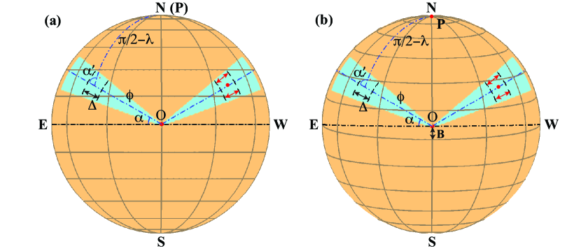
Figure 1: Time–distance helioseismic measurement schemes for the cases of (a) zero solar B-angle and (b) non-zero solar B-angle. In each blue-shaded area, we measure acoustic travel times between a pair of concentric arcs, which are at a distance of $\Delta$ apart and whose concentric center is at a distance of $\phi$ from the disk center. The line connecting the middle points of both arcs lie along the radial direction of the solar disk, with an angle of $\alpha$ relative to the disk’s apparent horizontal axis, and an angle of $\alpha^{\prime}$ relative to the local north at the concentric center.

Our new measurement strategy is to make exhaustive time–distance measurements for acoustic waves traveling between any two locations along solar disk’s radial direction. The measured quantities are travel-time shifts, $\delta\tau$, for a complete set of geometric parameters. As shown in the configuration in Figure 1, the acoustic source and receiver, represented by a pair of concentric arcs lying along the disk’s radial direction at an azimuthal angle $\alpha$ relative to the the disk’s apparent horizontal axis, are a great-circle distance $\Delta$ apart. The concentric center of the arc pair is at a great-circle distance of $\phi$ from the disk center, and each arc spans $30\arcdeg$ with a distance of $\Delta/2$ to the concentric center. To measure travel times for p-mode waves traveling between such a pair of arcs, we cross-correlate the two time sequences averaged from the Doppler signals in the two arcs. From the resulting cross-correlation functions we fit for wave-traveling times for both traveling directions using the Gabor wavelet function. To enhance the stability of the Gabor wavelet fitting, we average all the cross-correlation functions over a wedge of a $20\arcdeg$-wide azimuthal angle (see Figure 1) in each Carrington rotation, about 27 days.

The differences between the fitted travel times in the opposite traveling directions, $\delta\tau$, in principle contain contributions from various causes, listed in a magnitude-decreasing order: rotation, CtoL effect, meridional flow, and maybe some other yet unknown factors. To eliminate the rotation, we average the symmetric time-shift measurements on either side of the central meridian, as shown in Figure 1, since the projected components of the rotation along the two symmetric measurement directions are expected to have same values but opposite signs. The symmetrized time shift $\delta\tau(\alpha,\phi,\Delta)$ becomes rotation-free, and it can be related to the CtoL effect, $\delta\tau_{\mathrm{CtoL}}$, and the meridional-flow-induced travel-time shifts (as measured along latitudinal direction), $\delta\tau_{\mathrm{MF}}$, by a linear equation,

$$\delta\tau(\alpha,\phi,\Delta)=\delta\tau_{\mathrm{CtoL}}(\phi,\Delta)+\delta\tau_{\mathrm{MF}}(\lambda,\Delta)\,\cos\alpha^{\prime},$$ (1)

where $\lambda$ is latitude of the cocentric center of the arc pair, and $\alpha^{\prime}$ is the angle between the measurement direction (disk radial) and the local north direction (see Figure 1 and Equation 3). In this equation, the $\delta\tau_{\mathrm{CtoL}}$  is assumed azimuthally symmetric, i.e., invariant to azimuthal angle and varies only with $\phi$ and $\Delta$, and its validity will be examined later in §4. The $\delta\tau_{\mathrm{MF}}$  is longitudinal symmetric and varies with $\lambda$ and $\Delta$. When measured at an angle $\alpha^{\prime}$ relative to the local north, only the projection of meridional flow along the ray path contributes (under ray-path approximation as discussed in §4), i.e., the time-shift contribution to the measured time shift is $\delta\tau_{\mathrm{MF}}\,\cos\alpha^{\prime}$. On the observed disk with a solar B-angle $B$, the $\lambda$ and $\alpha^{\prime}$ in Equation 1 are given by a spherical geometric relation:

$$\lambda=\sin^{-1}{[\cos{\phi}\sin{B}+\sin{\phi}\cos{B}\sin{\alpha}]}$$ (2)

$$\alpha^{\prime}=\cos^{-1}{\bigg{[}\frac{\cos{\phi}\sin{\lambda}-\sin{B}}{\sin{\phi}\cos{\lambda}}\bigg{]}}.$$ (3)

Our processed data images are in the Postel’s projection coordinates, with the observed disk center as the coordinate origin, and the equator is off the apparent horizontal direction when the B-angle is non-zero. The CtoL effect depends on the location on the solar disk and is thus irrelevant to the solar B-angle, while the meridional flow is directly dependent on latitude that varies in the disk location with the B-angle. Therefore, the measurements at the same disk location over time cannot be averaged directly. However, since the B-angle varies slowly, we average the measurements for each Carrington rotation without expecting significant side effects, and the mean B-angle for each rotation is used when solving the equations above.

3 Data and Measurements

3.1 Data Preparation

We use 7 years of HMI full-disk Doppler-velocity data, from 2010 May 1 to 2017 April 30, for this analysis. The data are organized into 24-hr chunks with a 45-s cadence. The original data are first rebinned to $1024\times 1024$ pixels, and then tracked with the Carrington rotation rate and projected into Postel’s projection coordinates, with projected image center being the observed disk center. The tracked and remapped data are then rebinned again to a spatial resolution of $0\fdg 36$ pixel^-1 (here, $1\arcdeg$ is 1 heliographic degree) at the disk center in order to reduce the computational burden in the following time–distance computations while not losing resolution for the deep interior detections. We then get running-difference images, the difference between one image and the image immediately ahead of it, to reduce the effect of solar convection, so that the data can be used for helioseismic analysis without further filtering in the Fourier domain. An acoustic power map from one random date is shown in Figure 2b.

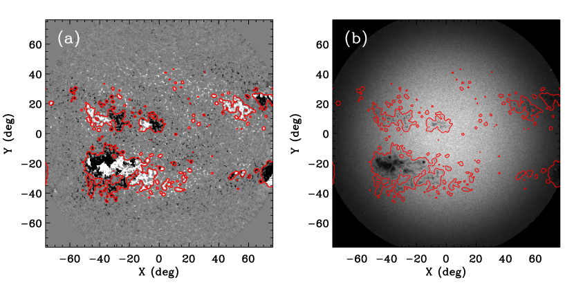
Figure 2: (a) Line-of-sight magnetic field image taken on 2012 July 8, with green contours of 10 G, inside which Doppler data are not used in our time–distance measurements. (b) Acoustic power map for the same date with the same contours over-plotted.

Another effect one needs to consider is the surface magnetic effect in helioseismic measurements, as recently demonstrated by Liang & Chou (2015a). The measured travel times for acoustic waves traveling into and out from a magnetic region exhibit a significant asymmetry that is, presumably, not accounted for by large-scale horizontal flows. This non-flow-related time shift will bias our meridional-flow-induced time-shift measurement notably if one end of the wave path is located inside a magnetic region. Therefore the magnetic regions should be masked to avoid such activity-related artifacts, as suggested by Liang & Chou (2015a). To prepare the masks, we track and remap the line-of-sight magnetic field data in the same way as for the Doppler-velocity data, but with a lower time step of 2 hours, and then average the daily images and smooth them using a normalized 2D Gaussian function kernel with a FWHM of $1\fdg 8$. Data falling into the area where magnetic field strength exceeds a threshold of 10 G will be masked and not used in the following helioseismic analysis. At most $14.5\%$ of the data pixels are masked during the solar maximum and a negligible number of pixels during the minimum years. The masking reduces the amount of data and boosts the noise level, therefore cannot be applied aggressively. The threshold of 10 G is so chosen that the deficit in acoustic power in and around the active regions are mostly covered, as shown in Figure 2.

3.2 Time–Distance Helioseismic Measurements

Following the measurement procedure prescribed in §2, one set of $\delta\tau(\alpha,\phi,\Delta)$ is obtained for each Carrington rotation starting from 2010 May 1, and a total of 93 rotations are obtained for the 7-yr period. Figure 3 shows the 7-yr-averaged $\delta\tau(\phi,\Delta)$ for the 6 azimuthal angle $\alpha$’s that are used in our following analysis. Since the east-west symmetric measurements (of $\alpha$ and $180\arcdeg-\alpha$) are folded to cancel the rotation, the final $\alpha$ only ranges from $0\arcdeg$ (east) to $90\arcdeg$ (north). All measurements in certain azimuthal wedges are binned into $\alpha=0\arcdeg,30\arcdeg,45\arcdeg,60\arcdeg,75\arcdeg$, and $90\arcdeg$, with $\alpha=15\arcdeg$ discarded due to that this azimuthal wedge mostly lie in the activity belts for many analysis periods and the measurement noises are much higher than for other $\alpha$’s.

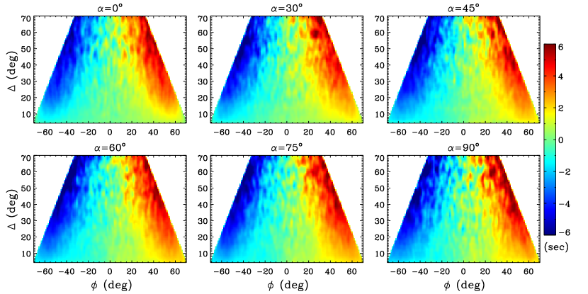
Figure 3: Seven-year averages of $\delta\tau$ measurements for each azimuthal angle $\alpha$ that is used in our analysis.

For each panel of Figure 3, the horizontal axis is the disk-centric distance $\phi$, ranging from $-65\arcdeg$ to $65\arcdeg$ with a distance sampling of $1\fdg 08$, and the vertical axis is skip distance $\Delta$, ranging from $4\fdg 32$ up to about $70\arcdeg$ with a step of $0\fdg 72$. The $\phi$ has positive sign in the northern hemisphere, and it is same as longitude in the case of $\alpha=0\arcdeg$, and same as latitude in the case of $\alpha=90\arcdeg$. The measurements have values in a trapezoid area because for larger measurement distances, one end of the measurement pair is too close to or out of the solar limb. The $\delta\tau$ is the difference between the two opposite traveling directions, with waves traveling from larger $\phi$ to smaller $\phi$ as positive direction.

All the panels in Figure 3 show a general anti-symmetric pattern with positive $\delta\tau$ for positive $\phi$ and vice versa. These panels are dominated by the CtoL effect, which exhibits as longer travel times along the direction from limb to disk center than along the opposite direction. The variations among different panels, most noticeable visually for small skip distances, are caused by the $\delta\tau_{\mathrm{MF}}$  projected into the disk’s radial direction. For $\alpha=0\arcdeg$, there is little contribution from the meridional flow to the measured $\delta\tau$, and the measurements were empirically used as the CtoL effect in the previous studies (e.g., Zhao et al., 2013), while for $\alpha=90\arcdeg$, $\delta\tau$ is a combination of the $\delta\tau_{\mathrm{CtoL}}$  and the $\delta\tau_{\mathrm{MF}}$. If only using measurements with $\alpha=0\arcdeg$ and $\alpha=90\arcdeg$, our method essentially reduces to the method of those previous time–distance studies, but with a couple of differences. One difference is that our measurements are always along the disk’s radial direction, while the previous authors measured along the north-south directions, which are off the radial direction except on the central meridian. The other difference is, the previous methods applied an averaging within a wide stripe, and the stripe was $30\arcdeg$-wide in longitude on the equator and $60\arcdeg$-wide in longitude at $65\arcdeg$ latitude. Our averaging is in a narrow $20\arcdeg$-wide azimuthal wedge, which is 1 pixel wide at the disk center and about $20\arcdeg$-wide in longitude at high-latitude regions. This narrower averaging pattern is designed for less overlapping in multiple-$\alpha$ measurements. However, we also realize that as a trade-off, our single-$\alpha$ measurement has larger noises for each individual wedge. Overall, our exhaustive measurements capture more information than the previous method on the intertwine of the $\delta\tau_{\mathrm{MF}}$  and $\delta\tau_{\mathrm{CtoL}}$  that the observations provide.

Due to the solar B-angle variation, throughout the 93 Carrington rotations, each pixel in the panels is measured at the same disk location $(\alpha,\phi)$ but not a same latitude. The maximum variation in latitude for one certain disk location can be $\pm 7.2\arcdeg$, and this effect is not negligible. Therefore, on the 7-yr-averaged images, shown in Figure 3, $\delta\tau_{\mathrm{CtoL}}$  are exactly averaged while $\delta\tau_{\mathrm{MF}}$  are smeared. Here we average these raw measurements to show the general patterns, but in the next section we solve a set of linear equations, given in Equation 1 – 3, with varying B-angles, to infer the $\phi$-dependent $\delta\tau_{\mathrm{CtoL}}$  and the latitude-dependent $\delta\tau_{\mathrm{MF}}$.

4 Disentangling CtoL Effect and Meridional-Flow-Induced Travel-Time Shifts

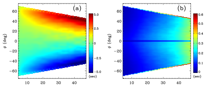
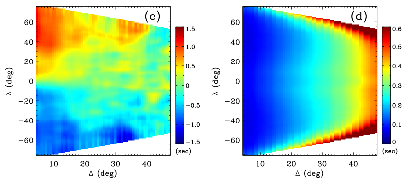
Figure 4: (a) CtoL effect $\delta\tau_{\mathrm{CtoL}}$ disentangled from our measurements. (b) Uncertainties of the $\delta\tau_{\mathrm{CtoL}}$. (c) Meridional-flow-induced travel-time shifts $\delta\tau_{\mathrm{MF}}$  disentangled from our measurements. (d) Uncertainties of the $\delta\tau_{\mathrm{MF}}$.

The $\delta\tau_{\mathrm{CtoL}}$  and $\delta\tau_{\mathrm{MF}}$  are disentangled by solving linear equations Equation 1 – 3. We observe that Equation 1 holds independently for each $\Delta$, that is, the subgroup of $\delta\tau(\alpha,\phi,\Delta)$ measured with a specific $\Delta$ forms a subset of linear equations, in which the unknown quantities $\delta\tau_{\mathrm{CtoL}}$  and $\delta\tau_{\mathrm{MF}}$  are both one-dimensional varying only with $\phi$ and $\lambda$, respectively. Besides, the combination of $\alpha$ and $\phi$ in $\delta\tau$ covers a wide range of $\phi$ and $\lambda$, and $\phi$ and $\lambda$ vary separately, making it an over-determined linear problem. We solve this over-determined one-dimensional linear equation set by employing a standard least-square method with a 2nd-order Tikhonov regularization on $\delta\tau_{\mathrm{CtoL}}$  and a 1st-order Tikhonov regularization on $\delta\tau_{\mathrm{MF}}$ (Aster et al., 2005). We assume $\delta\tau_{\mathrm{CtoL}}$  to be azimuthally symmetric, thus $\delta\tau_{\mathrm{CtoL}}$$=0$ at the disk center, and these prior information is incorporated as a constraint in the regularization as well.

Figure 4 shows the $\delta\tau_{\mathrm{CtoL}}(\Delta,\phi)$ and $\delta\tau_{\mathrm{MF}}(\Delta,\lambda)$, which are disentangled from our travel-time measurements through solving the linear equation set for the 7-yr period, and their uncertainties. The $\delta\tau_{\mathrm{CtoL}}$, of an order of 5 s, increases with skip distance $\Delta$ and disk-centric distance $\phi$, and its uncertainty increases with $\Delta$ as well. In each hemisphere, the $\delta\tau_{\mathrm{MF}}$, of an order of 1 s, shows a trend of decrease in magnitude with $\Delta$ within the range of $0\arcdeg$ to about $20\arcdeg$. Then the trend reverses to increase till the skip distance of about $35\arcdeg$. To show this trend more clearly, we plot the average curves of $\delta\tau_{\mathrm{MF}}$, for latitudinal bands of $10\arcdeg-30\arcdeg$ in both hemispheres (see Figure 5). The decreasing trend of magnitudes with skip distances smaller than $25\arcdeg$ indicates that the poleward flow becomes weaker or possibly turns equatorward at shallow depths. That the $\delta\tau_{\mathrm{MF}}$  curves bend back beyond a skip distance of $30\arcdeg$ indicates that the flow velocity reverses to poleward again below about 0.80 R_☉.

Figure 5: Average curves of $\delta\tau_{\mathrm{MF}}$ for $10\arcdeg-30\arcdeg$ latitudinal bands in both hemispheres.

As can be seen in Figure 4, at large skip distances the $\delta\tau_{\mathrm{MF}}$  is one order of magnitude smaller than $\delta\tau_{\mathrm{CtoL}}$, and the uncertainty of $\delta\tau_{\mathrm{MF}}$  increases greatly for large skip distances. Therefore the $\delta\tau_{\mathrm{MF}}$  beyond $\Delta=40\arcdeg$ are not used in our meridional-flow inversions in §5. We do not assume a hemispheric symmetry for the $\delta\tau_{\mathrm{MF}}$  when solving Equation 1, and the solved $\delta\tau_{\mathrm{MF}}$  indeed shows a north-south asymmetry, as can be seen in Figure 4c.

In Equation 1 – 3 the $\delta\tau_{\mathrm{CtoL}}$ is assumed azimuthally symmetric, and here we examine the validity of this assumption. If this assumption does not hold and $\delta\tau_{\mathrm{CtoL}}$ varies with $\alpha$, then Equation 1 cannot fit travel–time measurements well and the misfit shall show a dependence on $\alpha$. We examine the residues of fitting, $\delta\tau(\alpha,\phi,\Delta)-(\delta\tau_{\mathrm{CtoL}}(\phi,\Delta)+\delta\tau_{\mathrm{MF}}(\lambda,\Delta)\,\cos\alpha^{\prime})$, where $\delta\tau_{\mathrm{CtoL}}$ and $\delta\tau_{\mathrm{MF}}$ are solved from the linear regression. Figure 6a shows the distribution of the residues over different $\alpha$’s for $\phi=30\arcdeg$ and $\Delta$ between $14\fdg 4-21\fdg 6$. The box-plot shows the sample minimum, lower quartile, median, upper quartile, and maximum of the residues. The residues are randomly distributed and do not show any tendency with $\alpha$, indicating that the assumption of an isotropic CtoL is reasonable, i.e., the CtoL effect in the time–distance measurements using the HMI Doppler observations is azimuthally uniform within our measurement uncertainties. As another way to check, we examine the $\alpha$-dependent $\delta\tau_{\mathrm{CtoL}}$, which are obtained by subtracting the meridional-flow contribution $\delta\tau_{\mathrm{MF}}\cos\alpha^{\prime}$ (after $\delta\tau_{\mathrm{MF}}$ is solved) from the raw measurements of $\delta\tau$ for each $\alpha$. As shown in Figure 6b, for 3 selected skip distances, the CtoL effects agree well for different azimuthal angles.

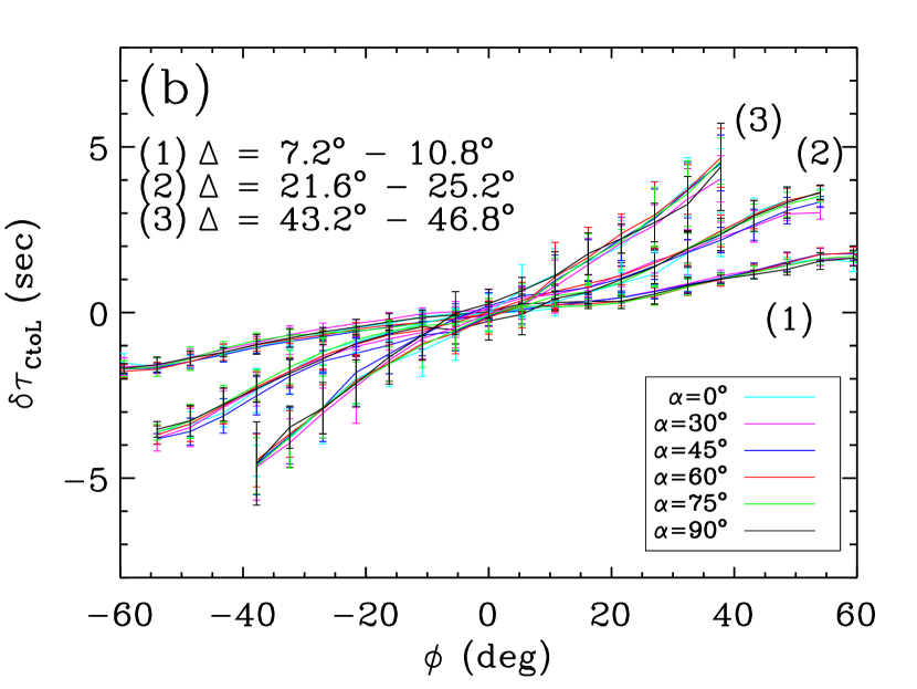
Figure 6: Left: Distribution of residues in model fitting, for $\phi=30\arcdeg$ and $\Delta$ falling between $14\fdg 4-21\fdg 6$. Right: CtoL effect derived for different $\alpha$’s for 3 skip-distance ranges.

5 Inverting for Meridional Flow

Meridional flow can be inverted from solving linear equations that relate the travel-time shifts $\delta\tau$, measured between two surface locations $\mathbf{x_{1}}$ and $\mathbf{x_{2}}$, and the flow velocity field $\mathbf{v}(\mathbf{r})$:

$$\delta\tau({\mathbf{x_{1}},\mathbf{x_{2}}})=2\int K(\mathbf{r},\Delta)\,\mathbf{v}(\mathbf{r^{\prime}}-\mathbf{r})\,\mathrm{d}\mathbf{r},$$ (4)

where $K(\mathbf{r},\Delta)$ is a three-dimensional flow sensitivity kernel for travel distance $\Delta$, which quantifies the amount of travel-time shifts caused by a localized unit flow, $\Delta=|\mathbf{x_{1}}-\mathbf{x_{2}}|$ is the great-circle distance between two surface locations $\mathbf{x_{1}}$ and $\mathbf{x_{2}}$, $\mathbf{r^{\prime}}=\frac{1}{2}(\mathbf{x_{1}}+\mathbf{x_{2}})$ is the midpoint of $\mathbf{x_{1}}$ and $\mathbf{x_{2}}$, and $\mathbf{r}$ is the offset between $\mathbf{r^{\prime}}$ and the flow location. Since the kernel $K(\mathbf{r},\Delta)$ is spherically symmetric for the same great-circle distance $\Delta$, it is denoted as $K_{\Delta}(\mathbf{r})$ hereafter. For $K_{\Delta}(\mathbf{r})$, we adopt the widely-used ray-path approximation kernels (e.g., Kosovichev, 1996; Zhao et al., 2013), in which the wavelength is assumed negligible relative to the flow length scale and the sensitivities concentrate only on ray paths. Ray-path approximations clearly have its limitation, and wave-based kernels, such as recently developed by Böning et al. (2016) and Gizon et al. (2017), will be used to replace the ray-path kernels in our future inversions.

In this paper, following practices by some previous authors (Zhao et al., 2013; Jackiewicz et al., 2015), we do not include radial flow $v_{r}$ in our inversions for the following reasons. First, the radial-flow-induced signals are expected to be at least one order of magnitude smaller than those caused by the meridional flow. Second, the travel-time shifts are only sensitive to the differences in radial flows, i.e., a uniform radial flow give zero time shifts since the effects along the upward and downward portions of the ray path get canceled. Third, cross talk between horizontal and radial flows, e.g., a downward flow and poleward flow in shallow interior for a poleward traveling wave play a same role in increasing $\delta\tau_{\mathrm{MF}}$, is another factor that complicates the inference of the radial flow.

Considering only the horizontal meridional flow $v_{\theta}$, Equation 4 can be rewritten as:

$$\delta\tau_{\mathrm{MF}}(\lambda,\Delta)=2\int K_{\Delta}(l,z)\,v_{\theta}(\lambda-l,z)\,\mathrm{d}l\mathrm{d}z,$$ (5)

where $z$ is depth and $l$ is latitudinal offset relative to the latitude $\lambda$. Under ray-path approximation, the sensitivities concentrate only on ray paths, so the three-dimensional kernel $K_{\Delta}(\mathbf{r})$ in Equation 4 reduces to a two-dimensional kernel $K_{\Delta}(l,z)$ in the meridional plane in Equation 5. Equation 5 is actually a convolution that can be more easily solved in the Fourier domain than in the space domain. In the Fourier domain, the equation can be written as:

$$\widehat{\delta\tau}_{\mathrm{MF}}(k,\Delta)=2\sum_{z}\widehat{v}(k,z)\,\widehat{K}_{\Delta}(k,z),$$ (6)

where   $\widehat{}$   denotes Fourier transform, and $k$ is spatial frequency in the latitudinal direction. It is clear that the equations become decoupled with $k$, and we get a one-dimensional linear equation for each $k$:

$$\widehat{\delta\tau}_{\mathrm{MF}}(\Delta)=2\sum_{z}\widehat{v}(z)\,\widehat{K}_{\Delta}(z).$$ (7)

We then solve each linear equation separately using a standard least-square solver with a 0th-order Tikhonov regularization (Aster et al., 2005). Since the radial flow is neglected in our equations, one should not expect the meridional flow $v$ obtained above to satisfy the local mass conservation. Instead, we consider a global mass conservation and limit the integrated mass flow on a latitudinal cross-section to be close to 0, similar to what Giles (1999) did. This is used as a constraint in our regularization as well.

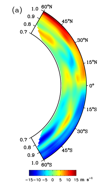
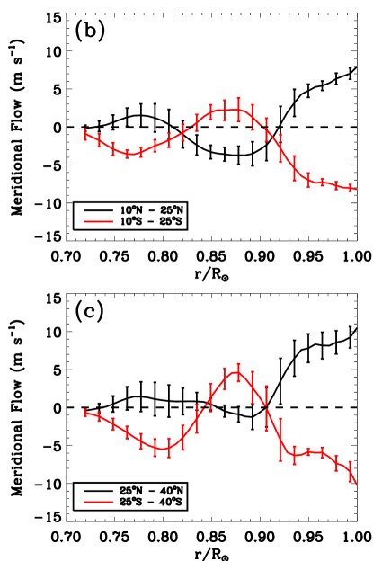
Figure 7: (a) Inverted meridional flow in the convection zone, with positive flow toward north. (b) Meridional-flow profile averaged from the $10\arcdeg-25\arcdeg$ latitudinal bands in both hemispheres. (c) Same as panel (b), but for the $25\arcdeg-40\arcdeg$ bands.

Figure 7 shows our inversion results. In both hemispheres for all latitudes, the poleward flow, of about $10$ m s^-1, extends from the surface to about 0.91 R_☉. Below 0.91 R_☉, the flow turns equatorward with a speed of about $5$ m s^-1, extending to about 0.82 R_☉ for low latitude regions, but not as deep for higher latitude. Beneath the layer of equatorward flow, the flow turns poleward again with a speed of lower than $5$ m s^-1. The averaged velocity profiles for 10$\arcdeg-25\arcdeg$ and 25$\arcdeg-40\arcdeg$ latitudinal bands, as shown in Figure 7b and 7c respectively, better illustrate the two direction reversals at depths of about 0.91 R_☉ and 0.82 R_☉ for 10$\arcdeg-25\arcdeg$ latitude, and 0.91 R_☉ and 0.85 R_☉ for 25$\arcdeg-40\arcdeg$ latitude. The northern and southern hemispheres exhibit an asymmetry in these inverted flow results. Compared with the southern hemisphere, the equatorward flow in the northern hemisphere extends into deeper convection zone, but does not span as wide in latitude.

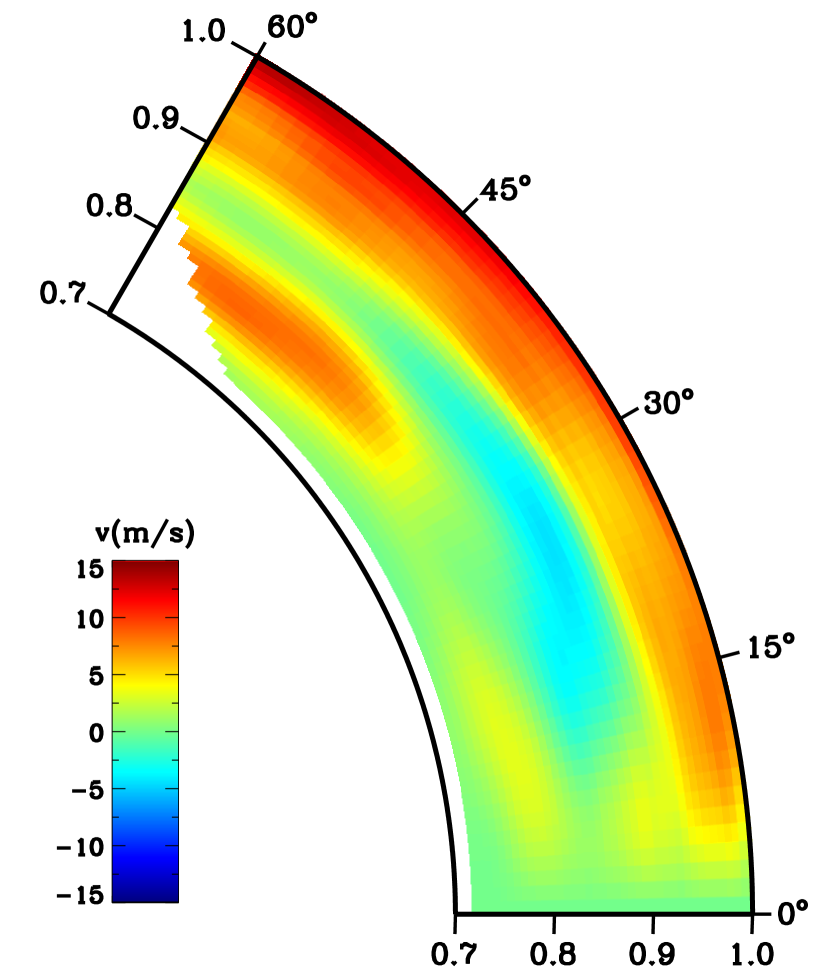
Figure 8: Hemispherically symmetrized meridional-flow profile. Positive flow is poleward and negative is equatorward.

To more clearly display the general pattern of the meridional circulation, we symmetrize the meridional-flow profiles of both hemispheres. The symmetrized profile (Figure 8) shows a 3-layer flow structure, indicating two circulation cells stacked in the radial direction in the convection zone. The surface poleward layer and the equatorward layer form the first circulation cell, and the lower part of the equatorward layer together with the deep poleward layer form the second cell, giving a picture consistent with the cartoon plot Figure 1 by Zhao et al. (2013).

6 Discussions

We have presented a new time–distance helioseismic measurement method to separate the systematic CtoL effect $\delta\tau_{\mathrm{CtoL}}$  and the meridional-flow-induced travel-time shifts $\delta\tau_{\mathrm{MF}}$. The new method measures exhaustively acoustic travel-time shifts along the solar disk’s all radial directions at all possible locations for all possible skip distances, and the $\delta\tau_{\mathrm{CtoL}}$  and $\delta\tau_{\mathrm{MF}}$  are disentangled from these measurements through solving a set of linear equations that relate these quantities to the measurements. The $\delta\tau_{\mathrm{MF}}$ are then used to invert for the Sun’s meridional circulation. Applying the new method on the 7-yr HMI Doppler observations, we are able to get a more robustly determined CtoL effect and a more accurately measured $\delta\tau_{\mathrm{MF}}$. The meridional circulation, inverted from the $\delta\tau_{\mathrm{MF}}$, exhibits essentially three flow layers that indicate a double-cell circulation in each hemisphere.

Our new measurement strategy is designed to give a more robust and accurate determination in the CtoL effect and thus the meridional flow than the previous method introduced in §1. As demonstrated in §4, the CtoL effect is isotropic relative to azimuthal angles, and this confirms the validity of the previous method – removing a CtoL effect proxy that is assessed using time-shift measurements along the equator. However, as we know, the final inference of the meridional flow relies strongly upon the accuracy of the effect removal, and a small error in the CtoL effect can cause a big error in the inverted flow. The CtoL effect obtained by our new method, disentangled from the exhaustive measurements throughout the entire solar disk along all radial directions, is more robust than the proxy in the previous method, which measures the CtoL effect in a narrow band in the equatorial area.

It is noticeable that our results on the meridional-circulation profile do not fully agree with any of the published results introduced in §1, but more similar to the result by Zhao et al. (2013) in the 3-layer flow structure, although our flow speed in the deepest layer is substantially slower than theirs. One possible reason that these two sets of results have more similarities than others is that, the analysis period by Zhao et al. (2013) was mostly during the solar minimum years, and magnetic field does not influence much on their final results, while our analysis largely remove the effects of the surface magnetic field following a method suggested by Liang & Chou (2015a). In this regard, the periods analyzed by both Jackiewicz et al. (2015) and Rajaguru & Antia (2015) have stronger magnetic activities that may complicate their final results. Meanwhile, it is not deniable that the major differences between our result and that of Rajaguru & Antia (2015) are likely caused by the inclusion of the radial flow and the mass-conservation condition in their inversion.

Some improvements can be made in our future efforts of inverting the $\delta\tau_{\mathrm{MF}}$  for the meridional circulation. One improvement is to include local-scale mass-conservation equations, for which the radial flow component is desired. We have reasonably neglected the radial component in this paper, but it is worth studying after a higher signal-to-noise ratio of the travel-time shifts is achieved in measurements and a method to disentangle the cross-talk between the horizontal and radial components is developed. Another recent development is the availability of the wave-based sensitivity kernels for the meridional flow in spherical coordinates. Böning et al. (2016) developed Born-approximation kernels and Gizon et al. (2017) developed wave-based kernels using numerical method, both of which are believed superior to the ray-approximation kernels that were used in the previous and current time–distance helioseismic inversions. These wave-based sensitivity kernels will be used in our future efforts.

Moreover, in this paper, only the 7-yr-averaged results are inverted and shown. However, as the Sun experienced from the activity minimum to the maximum and back toward the minimum again during these 7 years, the meridional circulation may have also experienced detectable changes. Armed with our new analysis method, we are capable of inferring the meridional flow for shorter periods and analyzing the temporal evolution of the Sun’s deep meridional circulation. That will offer us more knowledge of the Sun’s internal dynamics for a better understanding of the solar dynamo and its cycles.

References

- Aster et al. (2005) Aster, R. C., Borchers, B., & Thurber, C. H. 2005, Chapter 5, Parameter estimation and inverse problems, Elsevier Academic Press
- Basu & Antia (2003) Basu, S., & Antia, H. M. 2003, ApJ, 585, 553
- Böning et al. (2016) Böning, V. G. A., Roth, M., Zima, W., Birch, A. C., & Gizon, L. 2016, ApJ, 824, 49
- Braun & Fan (1998) Braun, D. C., & Fan, Y. 1998, ApJL, 508, L105
- Dikpati et al. (2010) Dikpati, M., Gilman, P. A., de Toma, G., & Ulrich, R. K. 2010, Geophys. Res. Lett., 37, L14107
- Duvall (1979) Duvall, T. L., Jr. 1979, Sol. Phys., 63, 3
- Duvall et al. (1993) Duvall, T. L., Jr., Jefferies, S. M., Harvey, J. W., & Pomerantz, M. A. 1993, Nature, 362, 430
- Featherstone & Miesch (2015) Featherstone, N. A., & Miesch, M. S. 2015, ApJ, 804, 67
- Giles (1999) Giles, P. M. 1999, PhD Thesis, Stanford Univ.
- Giles et al. (1997) Giles, P. M., et al. 1997, Nature, 390, 52
- Gizon et al. (2017) Gizon, L., Barucq, H., Duruflé, M., et al. 2017, A&A, 600, A35
- González Hernández et al. (1999) González Hernández, I., et al., 1999, ApJL, 510, L153
- Haber et al. (2000) Haber, D. A., Hindman, B. W., Toomre, J., et al. 2000, Sol. Phys., 192, 335
- Hartlep et al. (2013) Hartlep, T., Zhao, J., Kosovichev, A. G., & Mansour, N. N. 2013, ApJ, 762, 132
- Hathaway (1996) Hathaway, D. H. 1996, ApJ, 460, 1027
- Hathaway (2012) Hathaway, D. H. 2012, ApJ, 760, 84
- Hathaway & Rightmire (2010) Hathaway, D. H., & Rightmire, L. 2010, Science, 327, 1350
- Hill (1988) Hill, F. 1988, ApJ, 333, 996
- Howard & Gilman (1986) Howard, R., & Gilman, P. A. 1986, ApJ, 307, 389
- Jackiewicz et al. (2015) Jackiewicz, J., Serebryanskiy, A., & Kholikov, S. 2015, ApJ, 805, 133
- Komm et al. (1993) Komm, R. W., Howard, R. F., & Harvey, J. W. 1993, Sol. Phys., 147, 207
- Kholikov et al. (2014) Kholikov, S., Serebryanskiy, A., & Jackiewicz, J. 2014, ApJ, 784, 145
- Kosovichev (1996) Kosovichev, A. G. 1996, ApJL, 461, L55
- Liang & Chou (2015a) Liang, Z.-C., & Chou, D.-Y. 2015a, ApJ, 805, 165
- Liang & Chou (2015b) Liang, Z.-C., & Chou, D.-Y. 2015b, ApJ, 809, 150
- Meunier (1999) Meunier, N. 1999, ApJ, 527, 967
- Miesch (2005) Miesch, M. S. 2005, Living Rev. Solar Phys., 2, 1
- Parker (1955) Parker, E. N. 1955, ApJ, 122, 293
- Pesnell et al. (2012) Pesnell, W. D., Thompson, B. J., & Chamberlin, P. C. 2012, Sol. Phys., 275, 3
- Rajaguru & Antia (2015) Rajaguru, S. P., & Antia, H. M. 2015, ApJ, 813, 114
- Roth et al. (2016) Roth, M., Doerr, H.-P., & Hartlep, T. 2016, A&A, 592, A106
- Schad et al. (2011a) Schad, A., Roth, M., & Timmer, J. 2011, J. Phys. Conf. Ser., 271, 012079
- Schad et al. (2011b) Schad, A., Timmer, J., & Roth, M. 2011, ApJ, 734, 97
- Schad et al. (2013) Schad, A., Timmer, J., & Roth, M. 2013, ApJL, 778, L38
- Scherrer et al. (1995) Scherrer, P. H., Bogart, R. S., Bush, R. I., et al. 1995, Sol. Phys., 162, 129
- Scherrer et al. (2012) Scherrer, P. H., Schou, J., Bush, R. I., et al. 2012, Sol. Phys., 275, 207
- Schou et al. (2012) Schou, J., Scherrer, P. H., Bush, R. I., et al. 2012, Sol. Phys., 275, 229
- Švanda et al. (2007) Švanda, M., Zhao, J., & Kosovichev, A. G. 2007, Sol. Phys., 241, 27
- Ulrich (2010) Ulrich, R. K. 2010, ApJ, 725, 658
- Upton & Hathaway (2014a) Upton, L., & Hathaway, D. H. 2014a, ApJ, 780, 5
- Upton & Hathaway (2014b) Upton, L., & Hathaway, D. H. 2014b, ApJ, 792, 142
- Wang et al. (1989) Wang, Y.-M., Nash, A. G., & Sheeley, N. R., Jr. 1989, Science, 245, 712
- Wöhl & Brajša (2001) Wöhl, H., & Brajša, R. 2001, Sol. Phys., 198, 57
- Woodard (2000) Woodard, M. F. 2000, Sol. Phys., 197, 11
- Zhao & Kosovichev (2004) Zhao, J., & Kosovichev, A. G. 2004, ApJ, 603, 776
- Zhao et al. (2013) Zhao, J., Bogart, R. S., Kosovichev, A. G., Duvall, T. L., Jr., Hartlep, T. 2013, ApJL, 774, L29
- Zhao et al. (2012) Zhao, J., Nagashima, K., Bogart, R. S., Kosovichev, A. G., Duvall, T. L., Jr. 2012, ApJL, 749, L5