Azimuthal angle correlations at large rapidities: revisiting density variation mechanism

Abstract

In the paper we discuss the angular correlation present in hadron-hadron collisions at large rapidity difference ($\bar{\alpha}_{S}\,y_{12}\,\gg\,1$). We find that in the CGC/saturation approach the largest contribution stems from the density variation mechanism. Our principal results are that the odd Fourier harmonics ($v_{2n+1}$), decrease substantially as function of $y_{12}$, while the even harmonics ($v_{2n}$ ), increase considerably with a growth of $y_{12}$.

1 Introduction

In this paper we address the problem of the azimuthal angle correlations of two hadrons with transverse momenta $\vec{p}_{T1}$ and $\vec{p}_{T2}$ and rapidities $y_{1}$ and $y_{2}$, at large values of $y_{12}\equiv|y_{1}-y_{1}|\gg 1/\bar{\alpha}_{S}$. Our main theoretical assumption is that these correlations stem from interactions in the initial state. We are aware that, unlike rapidity correlations which at large rapidities are originated from the initial state interactions due to causality reasonsCAUSALITY , a substantial part of these correlations could be due to the interactions in the final statesFINSTATE . On the other hand, it has been demonstrated that at small rapidity difference $\bar{\alpha}_{S}\,y_{12}\,<\,1$ the interactions in the initial state RAJUREV ; KOLU1 ; KOWE ; KOLUCOR ; GLMT ; GLMBEH ; GOLE ; KOLULAST ; GLP gives the value of the correlations, which describe the major part of the experimentally observed correlationsCMSPP ; STARAA ; PHOBOSAA ; STARAA1 ; CMSPA ; CMSAA ; ALICEAA ; ALICEPA ; ATLASPP ; ATLASPA ; ATLASAA .

In this paper we concentrate our efforts, on calculating the long range rapidity part of angular correlations with large value of the rapidity difference $y_{12}$. All previous calculations, assumed that $\bar{\alpha}_{S}y_{12}\,<\,1$RAJUREV ; KOLU1 ; KOWE ; KOLUCOR ; GLMT ; GLMBEH ; GOLE ; KOLULAST ; GLP . It turns out, that in this kinematic region, the main source of the azimuthal angle correlations, is the Bose-Einstein correlations of identical gluons, which corresponds to the interference diagram in the production of two partonic showers. Intuitively, we expect that the correlations in the process, where two different gluons are produced from two different partonic showers, should not depend on the difference of rapidities ($y_{12}$), as well as on the values of $y_{1}$ and $y_{2}$. Using the AGK cutting rules AGK one can prove that the two gluon correlations can be calculated using the Mueller diagramsMUDIA of Fig. 1.

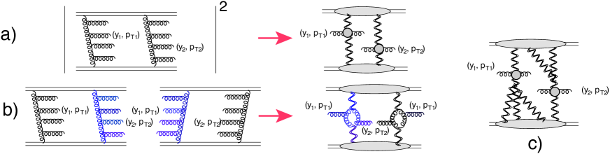
Figure 1: Mueller diagramsMUDIA for two partonic showers production. Fig. 1-a describes the square of the production amplitudes, while Fig. 1-b corresponds to the interference diagram which leads to the Bose-Einstein correlations. The wavy lines show the BFKL PomeronBFKL ; LI , while the helical lines denote gluons. Fig. 1-c shows the example of a more complicated structure of the partonic cascades, than the exchange of the BFKL Pomeron. The colour of the lines indicates the parton shower.

The diagrams of Fig. 1 lead to correlations which do not depend on $y_{1}$ and $y_{2}$, but only for $\bar{\alpha}_{S}\,y_{12}\,\ll\,1$. For large $y_{12}$ the contributions of Fig. 1 decrease. The main goal of this paper to find the contributions which survive at large $y_{12}$ ($\bar{\alpha}_{S}\,y_{12}\,\gg\,1$).

At large $y_{12}$, we have to take into account the emission gluons, with rapidities $y_{2}\,<\,y_{i}\,<\,y_{1}$ which transform the Mueller diagram of Fig. 1-b to more general diagrams of Fig. 2. The general features of Fig. 1-b is that the lower Pomerons carry momenta $\vec{Q}_{T}+\vec{p}_{12}$ and $-\vec{Q}_{T}-\vec{p}_{12}$ with $\vec{p}_{12}=\vec{p}_{T1}-\vec{p}_{T2}$. $\vec{Q}_{T}$ denotes the momentum along the BFKL Pomeron. After integration over $Q_{T}$, we obtain $p_{12}\sim 1/R_{h}$, where $R_{h}$ is the size of the target(projectile), which has a non-perturbative origin. Roughly speaking, the correlation function turns out to be proportional to $G\left(p_{12}\right)$, where $G$ denotes the non-perturbative form factor of the target or projectile GOLE . This conclusion stems from the value of the typical $Q_{T}$ for the BFKL Pomeron, which is determined by the size of the largest dipoles in the Pomeron. Fig. 2 does not have these features. We will show that the azimuthal angle correlations originate from the integration over $\vec{Q}_{T}$(see Fig. 2), due to the structure of the vertices of emission of the gluons with $\vec{p}_{T1}$ and $\vec{p}_{T2}$, which have contributions proportional to $(\vec{p}_{T1}\cdot\vec{Q}_{T})^{n}$ $(\vec{p}_{T2}\cdot\vec{Q}_{T})^{n}$. Recall, that these kind of vertices, are the only possibilities to obtain angular correlations in the classical Regge analysisKAID . This mechanism for azimuthal angular correlations was suggested in Ref.LERECOR (see also Refs.MLSK ; HHXY ; GLMT ; KOLUREV ), and in the review of Ref. KOLUREV , was called, the density variation mechanism.

The paper is organized as follows. In the next section we discuss the contribution of the diagram of Fig. 2 in the momentum representation. In the remainder of the paper, we will use the mixed representation: the dipole sizes and momentum transferred ($Q_{T}$), which will be introduced in section 3. Section 4 is devoted to the discussion of the single inclusive production in the Colour Glass Condensate (CGC)/saturation approach. The double inclusive production is considered in section 5, in which the rapidity dependence of the master diagram of Fig. 2 will be calculated. In section 6, we estimate the angular correlation function and Fourier harmonics $v_{n}$, and we present our prediction for dependence of $v_{n}$ on the difference of rapidities ($y_{12}$). In section 7 we draw our conclusions and outline problems for future investigation.

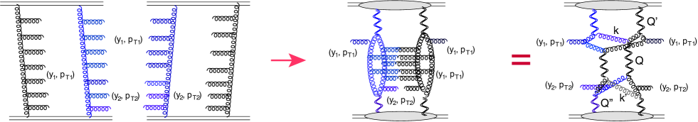
Figure 2: The generalization of Fig. 1-b for $\bar{\alpha}_{S}\,y_{12}\,\gg\,1$. The wavy lines show the BFKL PomeronBFKL ; LI , while the helical lines denote gluons. The colour (blue and black) of the lines indicates the parton shower.

2 Correlations in the momentum representation

The double inclusive cross section of Fig. 2 takes the following form

$$\frac{d^{2}\sigma}{dy_{1}d^{2}p_{T1}\,dy_{2}d^{2}p_{T2}}\left({Fig.~{}\ref{mudia}}\right)\,\,=\,\,\left(\frac{2C_{F}\alpha_{S}}{(2\pi)^{2}}\right)^{2}\int\frac{d^{2}k_{T}}{(2\pi)^{2}}\,\frac{d^{2}k^{\prime}_{T}}{(2\pi)^{2}}\,\frac{d^{2}Q^{\prime}_{T}}{(2\pi)^{2}}\,\frac{d^{2}Q_{T}}{(2\pi)^{2}}\,\frac{d^{2}Q^{\prime\prime}_{T}}{(2\pi)^{2}}\,k^{2}_{T}\,(\vec{k}_{T}-\vec{Q}_{T})^{2}$$ (2.1)

$$\times\,\,N\left(Q^{\prime}_{T}\right)\,\phi^{G}_{H}\left(-\vec{k}_{T}+\vec{Q}^{\prime}_{T},\vec{k}_{T};Y-y_{1}\right)\,\phi^{G}_{H}\left(\vec{k}_{T}-\vec{Q}_{T},-\vec{k}_{T}+\vec{Q}_{T}-\vec{Q}^{\prime}_{T};Y-y_{1}\right)\,\,\Gamma_{\nu}\left(-\vec{k}+\vec{Q}_{T},\vec{p}_{T1}\right)\,\Gamma_{\nu}\left(\vec{k}-\vec{Q}_{T}-\vec{Q}^{\prime}_{T},\vec{p}_{T1}\right)$$

$$\times\,\,\phi\left(-\vec{k}_{T},-\vec{k}_{T}+\vec{Q}_{T};\vec{k}^{\prime}_{t}+\vec{p}_{T2},-\vec{k}^{\prime}_{T}-\vec{p}_{2T}-\vec{Q}_{T};y_{12}\right)\,\phi\left(-\vec{k}_{T}+\vec{Q}^{\prime}_{T}+\vec{p}_{T1},\vec{k}_{T}-\vec{p}_{T1}-\vec{Q}_{T}-\vec{Q}^{\prime}_{T};\vec{k}^{\prime}_{T}-\vec{Q}^{\prime\prime}_{T}+\vec{Q}_{T},\vec{k}^{\prime}_{T}-\vec{p}_{T2};y_{12}\right)$$

$$\times\,\,N\left(Q^{\prime\prime}_{T}\right)\,\phi^{G}_{H}\left(\vec{k}^{\prime}_{T}-\vec{Q}^{\prime\prime}_{T}+\vec{Q}_{T},-\vec{k}^{\prime}_{T}-\vec{Q}_{T};y_{2}\right)\,\phi^{G}_{H}\left(-\vec{k}^{\prime}_{T}-\vec{Q}^{\prime\prime}_{T}+\vec{Q}_{T},\vec{k}^{\prime}_{T};y_{2}\right)\,\Gamma_{\mu}\left(-\vec{k}^{\prime}_{T}-\vec{p}_{T2}+\vec{Q}^{\prime\prime}_{T},\vec{p}_{T2}\right)\,\Gamma_{\mu}\left(\vec{k}^{\prime}_{T}-\vec{p}_{T2},\vec{p}_{T2}\right)$$

where $\phi^{G}_{H}\left(\vec{k}_{T},-\vec{k}+\vec{Q}_{T}^{\prime}\right)$, as well as all other functions $\phi$ of this type, are the correlation functions which at $Q^{\prime}_{T}=0$, give the probability to find a gluon with transverse momentum $\vec{k}_{T}$ in the hadron(nucleus) of the projectile (target). $\phi\left(\vec{k}_{T},-\vec{k}+\vec{Q}_{T};\vec{k}^{\prime}_{T},-\vec{k}^{\prime}_{T}+\vec{Q}_{T}\right)$ describes the interaction of two gluons with momenta $\vec{k}_{T}$ and $\vec{k}^{\prime}_{T}$, which scatter at momentum transferred $Q"_{T}$. $N\left(Q^{\prime}_{T}\right)$ is a pure phenomenological form factor that describes the probability to find two Pomerons in the projectile or target, with transferred moment $\vec{Q}^{\prime}_{T}$ and $-\vec{Q}^{\prime}_{T}$. $C_{F}\,=\,\left(N^{2}_{c}-1\right)/2N_{c}$ where $N_{c}$ is the number of colours. The Lipatov vertex $\Gamma_{\mu}\left(k_{T},p_{T1}\right)$ has the following form

$$\Gamma_{\mu}\left(k_{T},p_{T1}\right)\,\,=\,\,\frac{1}{p_{12}^{2}}\left(\,k^{2}_{T}\,p_{T1,\mu}\,-\,{k}_{T,\mu}\,p^{2}_{T1}\right);$$ (2.2)

Using Eq. (2.2) we obtain

$$2\,\Gamma_{\nu}\left(-\vec{k}+\vec{Q}_{T},\vec{p}_{T1}\right)\,\Gamma_{\nu}\left(\vec{k}-\vec{Q}_{T}-\vec{Q}^{\prime}_{T},\vec{p}_{T1}\right)\,=$$

$$\frac{1}{p^{2}_{T1}}\left(\left(-\vec{k}+\vec{Q}_{T}\right)^{2}\,\left(\vec{k}_{T}-\vec{p}_{T1}-\vec{Q}_{T}-\vec{Q}^{\prime}_{T}\right)^{2}\,+\,\left(-\vec{k}+\vec{p}_{T1}-\vec{Q}_{T}\right)^{2}\,\left(\vec{k}_{T}-\vec{Q}_{T}-\vec{Q}^{\prime}_{T}\right)^{2}\right)\,-\,Q^{\prime 2}_{T};$$

$$2\,\Gamma_{\mu}\left(-\vec{k}^{\prime}_{T}-\vec{p}_{T2}+\vec{Q}^{\prime\prime}_{T},\vec{p}_{T2}\right)\,\Gamma_{\mu}\left(\vec{k}^{\prime}_{T}-\vec{p}_{T2}-\vec{Q}_{T},\vec{p}_{T2}\right)\,=\,$$

$$\frac{1}{p^{2}_{T2}}\left(\left(-\vec{k}^{\prime}_{T}-\vec{p}_{T2}+\vec{Q}"_{T}\right)^{2}\left(\vec{k}^{\prime}_{T}-\vec{Q}_{T}\right)^{2}\,+\,\left(-\vec{k}^{\prime}_{T}+\vec{Q}^{\prime\prime}_{T}+\vec{Q}_{T}\right)^{2}\left(\vec{k}-\vec{p}_{T2}-\vec{Q}^{\prime\prime}_{T}\right)^{2}\right)\,-\,Q^{\prime\prime 2}_{T};$$ (2.3)

We can simplify the master equation (see Eq. (2.1) by observing, that dependence on $Q^{\prime}_{T}$ and $Q^{\prime\prime}_{T}$ is determined by the non-perturbative scale of the projectile(target) structure, which in Eq. (2.1), is absorbed in the phenomenological form factors $N(Q^{\prime}_{T})$ and $N(Q^{\prime\prime}_{T})$. Therefore, the typical $Q^{\prime}_{T}$ and $Q^{\prime\prime}_{T}$ turn out to be of the order of the soft scale $\mu_{\rm soft}$, which is much smaller that the other typical momenta in Eq. (2.1), assuming that $P_{T1}$ and $P_{T2}$ are larger than $\mu_{\rm soft}$. Introducing

$$\mu^{2}_{\rm soft}\,\,=\,\,\int\frac{d^{2}Q^{\prime}_{T}}{(2\,\pi)^{2}}N\left(Q^{\prime}_{T}\right)$$ (2.4)

we can neglect $Q^{\prime}_{T}$ and $Q^{\prime\prime}_{T}$ in the BFKL Pomeron Green’s functions and re- write Eq. (2.1) in the form:

$$\frac{d^{2}\sigma}{dy_{1}d^{2}p_{T1}\,dy_{2}d^{2}p_{T2}}\left({Fig.~{}\ref{mudia}}\right)\,\,=\,\,\left(\frac{2C_{F}\alpha_{S}\,\mu^{2}_{\rm soft}}{(2\pi)^{2}}\right)^{2}\int\frac{d^{2}k_{T}}{(2\pi)^{2}}\,\frac{d^{2}k^{\prime}_{T}}{(2\pi)^{2}}\,\,\frac{d^{2}Q_{T}}{(2\pi)^{2}}\,\,k^{2}_{T}\,(\vec{k}_{T}-\vec{Q}_{T})^{2}$$ (2.5)

$$\times\,\,\phi^{G}_{H}\left(-\vec{k}_{T},\vec{k}_{T};Y-y_{1}\right)\,\phi^{G}_{H}\left(\vec{k}_{T}-\vec{Q}_{T},-\vec{k}_{T}+\vec{Q}_{T};Y-y_{1}\right)\,\,\Gamma_{\nu}\left(-\vec{k}+\vec{Q}_{T},\vec{p}_{T1}\right)\,\Gamma_{\nu}\left(\vec{k}-\vec{Q}_{T},\vec{p}_{T1}\right)$$

$$\times\,\,\phi\left(-\vec{k}_{T},-\vec{k}_{T}+\vec{Q}_{T};\vec{k}^{\prime}_{t}+\vec{p}_{T2},-\vec{k}^{\prime}_{T}-\vec{p}_{2T}-\vec{Q}_{T};y_{12}\right)\,\phi\left(-\vec{k}_{T}+\vec{p}_{T1},\vec{k}_{T}-\vec{p}_{T1}-\vec{Q}_{T};\vec{k}^{\prime}_{T}+\vec{Q}_{T},\vec{k}^{\prime}_{T}-\vec{p}_{T2};y_{12}\right)$$

$$\times\,\,\phi^{G}_{H}\left(\vec{k}^{\prime}_{T}+\vec{Q}_{T},-\vec{k}^{\prime}_{T}-\vec{Q}_{T};y_{2}\right)\,\phi^{G}_{H}\left(-\vec{k}^{\prime}_{T}+\vec{Q}_{T},\vec{k}^{\prime}_{T};y_{2}\right)\,\Gamma_{\mu}\left(-\vec{k}^{\prime}_{T}-\vec{p}_{T2},\vec{p}_{T2}\right)\,\Gamma_{\mu}\left(\vec{k}^{\prime}_{T}-\vec{p}_{T2},\vec{p}_{T2}\right)$$

with Eq. (2) which takes the following form:

$$2\,\Gamma_{\nu}\left(-\vec{k}+\vec{Q}_{T},\vec{p}_{T1}\right)\,\Gamma_{\nu}\left(\vec{k}-\vec{Q}_{T},\vec{p}_{T1}\right)\,=\,$$

$$\frac{1}{p^{2}_{T1}}\left(\left(-\vec{k}+\vec{Q}_{T}\right)^{2}\,\left(\vec{k}_{T}-\vec{p}_{T1}-\vec{Q}_{T}\right)^{2}\,+\,\left(-\vec{k}+\vec{p}_{T1}-\vec{Q}_{T}\right)^{2}\,\left(\vec{k}_{T}-\vec{Q}_{T}\right)^{2}\right)\,-\,Q^{2}_{T};$$

$$2\,\Gamma_{\mu}\left(-\vec{k}^{\prime}_{T}-\vec{p}_{T2},\vec{p}_{T2}\right)\,\Gamma_{\mu}\left(\vec{k}^{\prime}_{T}-\vec{p}_{T2}-\vec{Q}_{T},\vec{p}_{T2}\right)\,=\,$$

$$\frac{1}{p^{2}_{T2}}\left(\left(-\vec{k}^{\prime}_{T}-\vec{p}_{T2}\right)^{2}\left(\vec{k}^{\prime}_{T}-\vec{Q}_{T}\right)^{2}\,+\,\left(-\vec{k}^{\prime}_{T}\right)^{2}\left(\vec{k}-\vec{p}_{T2}-\vec{Q}_{T}\right)^{2}\right)\,-\,Q^{2}_{T};$$ (2.6)

At high energies the parton densities $\phi(\dots;Y)$ in Eq. (2.1) and in Eq. (2.5), are proportional to $\exp\left(\Delta_{\rm BFKL}\,Y\right)$ for the BFKL Pomeron, where $\Delta_{BFKL}=2.8\,\bar{\alpha}_{S}$ is the intercept of the BFKL Pomeron. Bearing this in mind, one can see, that the interference diagram for the double inclusive cross section does not depend on $y_{1},y_{2}$ or on $y_{12}$.

The main diagram of Fig. 1-a, also does not depend on rapidities, and its expression has the following form:

$$\frac{d^{2}\sigma}{dy_{1}d^{2}p_{T1}\,dy_{2}d^{2}p_{T2}}\left({Fig.~{}\ref{becor}}-a\right)\,\,=\,\,\left(\frac{2C_{F}\alpha_{S}}{(2\pi)^{2}}\int d^{2}Q_{T}N^{2}\left(Q_{T}\right)\right)^{2}\int\frac{d^{2}k_{T}}{(2\pi)^{2}}\,\frac{d^{2}k^{\prime}_{T}}{(2\pi)^{2}}$$

$$\times\,\,\phi^{G}_{H}\left(-\vec{k}_{T},\vec{k}_{T};Y-y_{1}\right)\,\phi^{G}_{H}\left(\vec{k}_{T}-\vec{p}_{T1},-y_{2}\right)\,\,\Gamma_{\nu}\left(-\vec{k},\vec{p}_{T1}\right)\,\Gamma_{\nu}\left(\vec{k},\vec{p}_{T1}\right)$$

$$\times\,\,\varphi^{G}_{H}\left(-\vec{l}_{T},\vec{l}_{T};Y-y_{2}\right)\,\varphi^{G}_{H}\left(\vec{l}_{T}+\vec{p}_{T2},-\vec{l}_{T}-\vec{p}_{T2};y_{2}\right)\,\Gamma_{\mu}\left(\vec{l}_{T},\vec{p}_{T2}\right)\,\Gamma_{\mu}\left(-\vec{l}_{T},\vec{p}_{T2}\right)$$ (2.7)

3 BFKL Pomeron in the mixed representation

For a more convenient presentation, it turns out that the most economical way of calculating the diagram of Fig. 2, is to use the mixed representation of the BFKL Pomeron Green’s function, $G\left(\vec{r},\vec{R},\vec{Q}_{T},Y\right)$, where $r$ and $R$ are the sizes of two interacting dipoles , $Q_{T}$ denotes the momentum transferred by the Pomeron, and $Y$ the rapidity between the two dipoles. This Green’s function is well knownLI and we discuss it here for the completeness of presentation, referring to Refs.LI ; NAPE for all details. It has the following form:

$$G\left(\vec{r},\vec{R},\vec{Q}_{T};Y\right)\,\,=\,\,\frac{r\,R}{16}\sum^{\infty}_{n=-\infty}\int^{\infty}_{-\infty}d\nu\frac{1}{\left(\nu^{2}+\frac{1}{4}(n-1)^{2}\right)\,\left(\nu^{2}+\frac{1}{4}(n+1)\right)}V_{\nu,n}\left(\vec{r},\vec{Q}_{T}\right)\,V^{*}_{\nu,n}\left(\vec{R},\vec{Q}_{T}\right)\,e^{\omega\left(\nu,n\right)\,Y}$$ (3.8)

where

$$\omega\left(\nu,n\right)\,\, = \,\,2\,\bar{\alpha}_{S}{\rm Re}\left(\psi\left(\frac{1}{2}+\frac{1}{2}|n|+\nu\right)-\psi\left(1\right)\right);$$

$$\omega\left(\nu,0\right)\,\, = \,\,2\,\bar{\alpha}_{S}{\rm Re}\left(\psi\left(\frac{1}{2}++\nu\right)-\psi\left(1\right)\right)\,\,\xrightarrow{\nu\ll 1}\,\,\Delta_{\rm BFKL}\,\,-\,\,D\,\nu^{2};$$ (3.9)

where $\psi(z)$ is the Euler $\psi$-function (see Ref.RY formulae 8.36) and $\Delta_{\rm BFKL}=\bar{\alpha}_{S}4\ln 2,D=\bar{\alpha}_{S}14\zeta(3),\xi=\ln\left(r^{2}_{1}/r^{2}_{2}\right)$.

Each term in Eq. (3.8) has a very simple structure, being the typical contribution of the Regge pole exchange: the product of two vertices and Regge-pole propagator. From Eq. (3) one can see that at large $Y$ the main contribution comes from the term with $n=0,$ and in what follows we will concentrate on this particular term. The vertices with $n=0$ have been determined in Refs.LI ; NAPE , and they have an elegant form in the complex number representation for the point on the two dimensional plane: viz.

$$\mbox{For }\vec{r}(x,y):\,\,\rho=x+iy;\,\,\rho^{*}=x-iy;~{}~{}~{}~{}~{}\mbox{For }\vec{Q}_{T}(Q_{x},Q_{y}):\,\,q=Q_{x}+iQ_{y};\,\,q^{*}=Q_{x}-iQ_{y};$$ (3.10)

Using this notation the vertices have the following structure:

$$V_{\nu}\left(\vec{r},\vec{Q}_{T}\right)\,=\,\left(Q^{2}_{T}\right)^{i\nu}\,\Gamma^{2}\left(1-i\nu\right)\Bigg{\{}J_{-i\nu}\left(\frac{1}{4}q^{*}\rho\right)\,J_{-i\nu}\left(\frac{1}{4}q\rho^{*}\right)\,\,-\,\,J_{i\nu}\left(\frac{1}{4}q^{*}\rho\right)\,J_{i\nu}\left(\frac{1}{4}q\rho^{*}\right)\Bigg{\}}$$ (3.11)

At $Q_{T}\to 0$ this vertex takes the form:

$$2^{6i\nu}\,V_{\nu}\left(\vec{r},\vec{Q}_{T}\right)\,\xrightarrow{Q_{T}r\,\ll\,1}$$ (3.12)

$$\left(\frac{r^{2}}{2^{6}}\right)^{-i\nu}\left(\frac{(\nu+i)\left(8(\vec{Q}_{T}\cdot\vec{r})^{4}-8(\vec{Q}_{T}\cdot\vec{r})^{2}Q^{2}_{T}r^{2}+5\frac{1}{2}Q^{4}_{T}r^{4}\right)+(2i+\nu)Q^{4}_{T}r^{4})}{64^{2}(\nu+2i)(1-i\nu)^{2}}+\frac{i(\nu+i)\left((2(\vec{Q}_{T}\cdot\vec{r})^{2}-Q^{2}_{T}r^{2}\right)}{32(1-i\nu)^{2}}+1\right)$$

$$+\left(Q^{2}\right)^{i\nu}\left(\frac{Q^{2}r^{2}}{2^{6}}\right)^{i\nu}\left(\frac{(\nu-2i)\left(8(\vec{Q}_{T}\cdot\vec{r})^{4}-8(\vec{Q}_{T}\cdot\vec{r})^{2}Q^{2}_{T}r^{2}+5\frac{1}{2}Q^{4}_{T}r^{4}\right))}{2^{12}((2+i\nu)(1+i\nu))^{2}}+\frac{2(1+i\nu)\left((2(\vec{Q}_{T}\cdot\vec{r})^{2}-Q^{2}_{T}r^{2}\right)}{2^{6}(1+i\nu)^{2}}-1\right)$$

For small values of $\nu$ (which are related to the region of large $\bar{\alpha}_{S}Y\,\gg\,1$), Eq. (3.12) can be simplified and reduced to the form:

$$2^{6i\nu}V_{\nu}\left(\vec{r},\vec{Q}_{T}\right)\,\xrightarrow{Q_{T}r\,\ll\,1}$$ (3.13)

$$\left(\frac{r^{2}}{2^{6}}\right)^{-i\nu}\left(\frac{(\vec{Q}_{T}\cdot\vec{r})^{4}-(\vec{Q}_{T}\cdot\vec{r})^{2}Q^{2}_{T}r^{2}+\frac{9}{16}Q^{4}_{T}r^{4})}{2^{8}}-\frac{2(\vec{Q}_{T}\cdot\vec{r})^{2}-Q^{2}_{T}r^{2}}{2^{5}}+1\right)$$

$$-\,\left(Q^{2}\right)^{i\nu}\left(\frac{Q^{2}r^{2}}{2^{6}}\right)^{i\nu}\left(\frac{(\vec{Q}_{T}\cdot\vec{r})^{4}-(\vec{Q}_{T}\cdot\vec{r})^{2}Q^{2}_{T}r^{2}+\frac{9}{16}Q^{4}_{T}r^{4})}{2^{8}}-\frac{2(\vec{Q}_{T}\cdot\vec{r})^{2}-Q^{2}_{T}r^{2}}{2^{5}}+1\right)$$

Using that

$$J_{-i\nu}\left(z\right)\,\,\xrightarrow{z\,\gg\,1}\,\,\sin\left(\frac{1}{4}\pi+z+\frac{1}{2}i\pi\nu\right)\sqrt{\frac{2}{\pi}}\sqrt{\frac{1}{z}}$$ (3.14)

at $\nu\ll 1$ we obtain for $Q^{2}_{T}r^{2}\gg 1$

$$V_{\nu}\left(\vec{r},\vec{Q}_{T}\right)\,\,\xrightarrow{Q_{T}r\,\gg\,1}\,\,\left(Q^{2}_{T}\right)^{i\nu}\,\Gamma^{2}\left(1-i\nu\right)\,\,\cos\left(\frac{1}{2}\vec{Q}_{T}\cdot\vec{r}\right)\,\frac{4\,i\,\nu}{Q_{T}\,r}$$ (3.15)

The contribution of the first term in Eq. (3.8) can be reduced to the following form for the scattering amplitude of two dipoles with sizes $r_{1}$ and $r_{2}$:

$$N\left(r_{1},r_{2};Y\right)\,\, = \,\,\frac{r_{1}\,r_{2}}{16}\int d\nu\frac{1}{\left(\nu^{2}+1/4\right)^{2}}\,V_{\nu}\left(r_{1},Q_{t}\to 0\right)V^{*}_{\nu}\left(r_{2},Q_{T}\to 0\right)\,e^{\omega\left(\nu,0\right)Y}$$ (3.16)

$$= \,\,\frac{r_{1}\,r_{2}}{16}\int d\nu\frac{1}{\left(\nu^{2}+1/4\right)^{2}}\,e^{\omega\left(\nu,0\right)Y}\Bigg{\{}(r^{2}_{1})^{-i\nu}-\left(\frac{Q^{4}_{T}r^{2}_{1}}{2^{12}}\right)^{i\nu}\Bigg{\}}\,\Bigg{\{}(r^{2}_{2})^{i\nu}-\left(\frac{Q^{4}_{T}r^{2}_{2}}{2^{12}}\right)^{-i\nu}\Bigg{\}}$$

$$= \,\,\frac{r_{1}\,r_{2}}{16}\int d\nu\frac{1}{\left(\nu^{2}+1/4\right)^{2}}\,e^{\omega\left(\nu,0\right)Y}2\left(\frac{r^{2}_{2}}{r^{2}_{1}}\right)^{i\nu}$$

$$\xrightarrow{Y\gg 1;\nu\ll 1} \,\,2\,r_{1}\,r_{2}\int d\nu\exp\left(\left(\bar{\alpha}_{S}\,4\ln 2\,-\bar{\alpha}_{S}14\zeta(3)\nu^{2}\right)Y\right)\left(\frac{r^{2}_{2}}{r^{2}_{1}}\right)^{i\nu}$$

$$= r_{1}\,r_{2}\sqrt{\frac{2\pi}{DY}}\exp\left(\Delta_{\rm BFKL}Y-\frac{\xi^{2}}{4DY}\right)$$

where $\Delta_{\rm BFKL}$ and $D$ are defined in Eq. (3).

In the derivation of Eq. (3.16) we neglected the contributions that are proportional to $\left(\frac{Q^{4}_{T}r^{2}_{2}\,r^{2}_{1}}{2^{12}}\right)^{-i\nu}$ since this contribution will be the same as in Eq. (3.16), but with, $\xi=\ln\left(\frac{Q^{4}_{T}r^{2}_{2}\,r^{2}_{1}}{2^{12}}\right)\,\gg\,1$. To integrate over $\nu$, we use the method of steepest descent, and the expansion of $\omega\left(\nu,0\right)$ at small $\nu$ (diffusion approximation, see the second equation in Eq. (3)).

$N\left(r_{1},r_{2};Y\right)$ denotes the imaginary part of the dipole-dipole sacttering amplitude at $Q_{T}=0$, which is related to the cross section. One can check that Eq. (3.16) has the correct dimension.

4 Single inclusive production in a one parton shower

4.1 BFKL Pomeron: the simplest approach for a one parton shower

The single inclusive cross section resulting from the one BFKL Pomeron is known, and it is equal to

$$\frac{d^{2}\sigma}{dyd^{2}p_{T}}\,\,=\,\,\frac{2C_{F}\alpha_{S}}{(2\pi)^{2}}\int\frac{d^{2}d^{2}k_{T}}{(2\pi)^{2}}\phi^{G}_{H}\left(\vec{k}_{T},Q_{T}=0;Y-y\right)\phi^{G}_{H}\left(\vec{k}_{T}-\vec{p}_{T},Q_{T}=0;y\right)\,\Gamma_{\nu}\left(\vec{k}_{T},\vec{p}_{T}\right)\,\Gamma_{\nu}\left(-\vec{k}_{T},\vec{p}_{T}\right)$$ (4.17)

The relation between the parton densities $\phi$ and the Green’s function of the BFKL Pomeron has been given in Ref.AGK2 :

$$N^{\rm\tiny BFKL}\left(r,r_{1};y,Q_{T}=0\right)\,\,=\,\,\frac{\alpha_{S}}{2}\int d^{2}k_{T}\,\left(1\,-\,e^{i\vec{k}_{T}\cdot\vec{r}}\right)\,\frac{\phi^{G}_{H}\left(\vec{k}_{T},Q_{T}=0;y\right)}{k^{2}_{T}}$$ (4.18)

where $N^{\rm\tiny BFKL}\left(r,r_{1};Y\right)$ is given by Eq. (3.8) or by Eq. (3.16), in the high energy limit. Eq. (4.18) can be re-written as follow

$$\phi^{G}_{H}\left(\vec{k}_{T},Q_{T}=0;y\right)\,\,=\,\,\frac{2}{\alpha_{S}}\int d^{2}e^{i\vec{k}_{T}\cdot\vec{r}}\,\nabla^{2}_{r}\,N^{\rm\tiny BFKL}\left(r,r_{1};y,Q_{T}=0\right)$$ (4.19)

We have

$$\Gamma_{\nu}\left(\vec{k}_{T},\vec{p}_{T}\right)\,\Gamma_{\nu}\left(-\vec{k}_{T},\vec{p}_{T}\right)\,\,=\,\,\frac{k^{2}_{T}\,\left(\vec{k}_{T}-\vec{p}_{T}\right)^{2}}{p^{2}_{T}}$$ (4.20)

Plugging in Eq. (4.18) and Eq. (4.20) into Eq. (4.17) we obtain AGK2

$$\frac{d^{2}\sigma}{dy\,d^{2}p_{T}}\,\,=\,\,\frac{8C_{F}}{\alpha_{S}\,(2\pi)^{2}}\frac{1}{p^{2}_{T}}\int d^{2}r\,e^{i\vec{p}_{T}\cdot\vec{r}}\,\nabla^{2}_{r}\,N^{\rm\tiny BFKL}_{\rm pr}\,\left(r,r_{1};Y-y,Q_{T}=0\right)\,\nabla^{2}_{r}\,N^{\rm\tiny BFKL}_{\rm tr}\,\left(r,r_{2};y,Q_{T}=0\right)$$ (4.21)

where $N_{\rm pr}$ and $N_{\rm tr}$ denote the probability to find a dipole in the projectile and target, respectively. $r_{1}$ and $r_{2}$ are the typical dipoles sizes in the projectile and target.

As can be seen from Eq. (2.1) we need to generalize Eq. (4.21) for the case $Q_{T}\neq 0$. Eq. (4.17) has to be replaced by

$$\frac{d^{2}\sigma}{dyd^{2}p_{T}}\left(Q_{T}\neq 0\right)\,\,=$$ (4.22)

$$\frac{2C_{F}\alpha_{S}}{(2\pi)^{2}}\int\frac{d^{2}k_{T}}{(2\pi)^{2}}\phi^{G}_{H}\left(\vec{k}_{T},Q_{T},Y-y\right)\phi^{G}_{H}\left(\vec{k}_{T}-\vec{p}_{T},Q_{T};y\right)\,\Gamma_{\nu}\left(\vec{k}_{T},\vec{p}_{T}\right)\,\Gamma_{\nu}\left(-\vec{k}_{T}+\vec{Q}_{T},\vec{p}_{T}\right)$$

Taking into account Eq. (4.18) for $Q_{T}\neq 0$ and

$$\Gamma_{\nu}\left(\vec{k}_{T},\vec{p}_{T}\right)\,\Gamma_{\nu}\left(-\vec{k}_{T}+\vec{Q}_{T},\vec{p}_{T}\right)\,\,=\,\,\frac{1}{2}\Bigg{\{}\frac{1}{p^{2}_{T}}\Bigg{[}\left(\vec{k}_{T}-\vec{Q}_{T}\right)^{2}\left(\vec{k}_{T}-\vec{p}_{T}\right)^{2}\,\,+\,\,\left(\vec{k}_{T}\right)^{2}\left(\vec{k}_{T}-\vec{p}_{T}-\vec{Q}_{T}\right)^{2}\Bigg{]}\,\,-\,\,Q^{2}_{T}\Bigg{\}}$$ (4.23)

we re-write Eq. (4.21) in the form

$$\frac{d^{2}\sigma}{dy\,d^{2}p_{T}}\left(Q_{T}\neq 0\right)\,\, = \,\,\frac{4C_{F}}{\alpha_{S}\,(2\pi)^{2}}\frac{1}{p^{2}_{T}}\int d^{2}r\,e^{i\vec{p}_{T}\cdot\vec{r}}$$

$$\times \Bigg{\{}-\nabla^{2}_{r}\,N^{\rm\tiny BFKL}_{\rm pr}\,\left(r,r_{1};Y-y,Q_{T}\right)\,(-i\nabla_{r}\,-\,\vec{Q}_{T})^{2}\,N^{\rm\tiny BFKL}_{\rm tr}\,\left(r,r_{2};y,Q_{T}\right)\,$$

$$+ \,(-i\nabla_{r}\,-\,\vec{Q}_{T})^{2}\,(-\nabla^{2}_{r})N^{\rm\tiny BFKL}_{\rm pr}\,\left(r,r_{1};Y-y,Q_{T}\right)\,\,N^{\rm\tiny BFKL}_{\rm tr}\,\left(r,r_{2};y,Q_{T}\right)\Bigg{\}}$$

$$- \,\,Q^{2}_{T}\frac{4C_{F}}{\alpha_{S}\,(2\pi)^{2}}\int d^{2}r\,e^{i\vec{p}_{T}\cdot\vec{r}}\,N^{\rm\tiny BFKL}_{\rm pr}\,\left(r,r_{1};Y-y,Q_{T}\right)\,N^{\rm\tiny BFKL}_{\rm tr}\,\left(r,r_{2};y,Q_{T}\right)$$

4.2 General estimates

It should be stressed that the single inclusive production has the form of Eq. (4.21) and Eq. (4.1) as was shown in Ref.AGK2 for the general structure of the single parton shower. For example, for the process shown in Fig. 1-c. We need only to substitute $N^{G}_{\rm tr}\,\left(r,r_{2};y,Q_{T}\right)$ for $2N^{\rm\tiny BFKL}_{\rm tr}\,\left(r,r_{2};y,Q_{T}\right)$ where

$$2N^{\rm\tiny BFKL}_{\rm tr}\,\left(r,r_{2};y,Q_{T}\right)\,\,\to\,\,N^{G}_{\rm tr}\,\left(r,r_{2};y,Q_{T}\right)\,\,=\,\,2N_{\rm tr}\,\left(r,r_{2};y,Q_{T}\right)-\int d^{2}Q^{\prime}_{T}\,N_{\rm tr}\,\left(r,r_{2};y,\vec{Q}_{T}-\vec{Q}^{\prime}_{T}\right)\,N_{\rm tr}\,\left(r,r_{2};y,\vec{Q}^{\prime}_{T}\right)$$ (4.25)

$N_{\rm tr}\,\left(r,r_{2};y,Q_{T}\right)$ is a solution to the non-linear evolution equation. For the case of inclusive production, we can considerably simplify estimates noting that

$$\nabla^{2}_{r}\,N_{\rm tr}\,\left(r,r_{2};y,Q_{T}\right)\xrightarrow{r^{2}Q^{2}_{s}\left(y\right)\,\ll\,1}\,\,\,N^{\rm BFKL}_{\rm tr}\,\left(r,r_{2};y,Q_{T}\right)\,\,\ll\,\,1;~{}~{}~{}~{}\nabla^{2}_{r}\,N_{\rm tr}\,\left(r,r_{2};y,Q_{T}\right)\xrightarrow{r^{2}Q^{2}_{s}\left(y\right)\,\gg\,1}\,\,0;$$ (4.26)

where $Q_{s}(y)$ denotes the saturation momentum.

In other words, the main contribution to inclusive production comes from the vicinity of the saturation scale, where $r^{2}Q^{2}_{s}\approx\,1$. Fortunately, the behavior of $N$ in this kinematic region is determined by the linear BFKL evolution equation GLR ; MUQI ; MV and has the following formMUTR

$$N_{\rm tr}\,\left(r,r_{2};y,Q_{T}=0\right)\,\,\propto\,\,\left(r^{2}Q^{2}_{s}(y)\right)^{1-\gamma_{cr}}~{}\mbox{with}~{}~{}Q^{2}_{s}=(1/r^{2}_{2})\,\exp\left(\frac{\omega\left(\gamma=\frac{1}{2}+i\nu=\gamma_{cr}\right)}{1-\gamma_{cr}}\,y\right)\,=\,(1/r^{2}_{2})e^{\kappa\,y}$$ (4.27)

where $\gamma_{cr}$ = 0.37.

We have seen in Eq. (3.15) that for $Q_{T}\neq 0$ , the scattering amplitude decreases at $Q^{4}_{T}\,r^{2}\,r^{2}_{2}\,\gg\,1$. Therefore, we need to consider rather small values of $Q_{T}$: $Q^{4}_{T}\,r^{2}\,r^{2}_{2}\,\leq\,1$. The product of vertices that determines the amplitude has two terms ( see Eq. (3.12) ) which are proportional to $\left(r^{2}/r^{2}_{2}\right)^{i\nu}$ and to $\left(Q^{4}_{T}\,r^{2}\,r^{2}_{2}\right)^{I\nu}$. Therefore, the maximum of $\nabla^{2}_{r}N$ can be reached if $r^{2}/r^{2}_{2}e^{\kappa\,y}\,\sim\,1$ and $Q^{4}_{T}\,r^{2}\,r^{2}_{2}e^{\kappa\,y}\,\sim\,1$ and the amplitude then has the following form

$$N_{\rm tr}\,\left(r,r_{2};y,Q_{T}\right)\,\,\propto\,\,c_{1}\left(\frac{r^{2}}{r^{2}_{2}}e^{\kappa\,y}\right)^{1-\gamma_{cr}}\,\,+\,\,c_{2}\left(Q^{4}_{T}\,r^{2}\,r^{2}_{2}\,e^{\kappa\,y}\right)^{1-\gamma_{cr}}$$ (4.28)

The first term does not depend on $Q_{T}$ and, therefore, the upper limit of the integral over $Q_{T}$, goes up to $\left(Q^{max}_{T}\right)^{2}\,\approx 1/(r\,r_{2})$. The second term both for $Q^{2}_{T}\,r\,r_{2}\,<\,e^{-\frac{1}{2}\kappa\,y}$ and for $Q^{2}_{T}\,r\,r_{2}\,>\,e^{-\frac{1}{2}\kappa\,y}$ turns out to be small. Indeed, in the first region the amplitude is small, while in the second region we are deep in the saturation domain where $\nabla^{2}_{r}N\to 0$. Hence, we expect that in the integral over $Q_{T}$, the first term gives a larger contribution than the second term and we will keep only this contribution in our estimates.

5 Double inclusive cross section for two parton shower production

5.1 The simplest diagram

In this section we calculate the simplest diagram of Fig. 2. We need to integrate the product of two BFKL Pomerons over $Q_{T}$ (see Eq. (2.5)):

$$I\,\,=\,\,\int d^{2}Q_{T}\,V_{\nu_{1}}\left(\vec{r}_{1},\vec{Q}_{T}\right)\,V^{*}_{\nu_{1}}\left(\vec{r}_{2},\vec{Q}_{T}\right)\,V_{\nu_{2}}\left(\vec{r}^{\prime}_{1},\vec{Q}_{T}\right)\,V^{*}_{\nu_{2}}\left(\vec{r}^{\prime}_{2},\vec{Q}_{T}\right)$$ (5.29)

From Eq. (2.5) in the momentum representation, we see that $r_{1}\,\neq\,r^{\prime}_{1}$($r_{2}\,\neq\,r^{\prime}_{2}$ ) but they are close to each other, being determined by the same momentum $k_{T}$. We assume that $p_{T1}<k_{T}$, since $k_{T}\sim Q_{s}\left(Y-y_{1}\right)\gg\mu_{\rm soft}$. Considering $r_{1}\approx r^{\prime}_{1}\,\ll\,r_{2}\approx r^{\prime}_{2}$ we will show that in the integral over $Q_{T}$, the typical $Q_{T}\sim 1/r_{2}$. In other words, the dependence of $Q_{T}$ is determined by the largest of interacting dipoles.

From Eq. (3.15) we see that for large $Q_{T}$, when $r^{2}_{1}Q^{2}_{T}\,\gg\,1$ and $r^{2}_{2}\,Q^{2}_{T}\,\gg\,1$, the integrand is proportional to $1/Q^{4}_{T}$, and converges. The main region of interest is $r^{2}_{2}\,Q^{2}_{T}\,\gg\,1$ and $r^{2}_{1}\,Q^{2}_{T}\,\ll\,1$. In this kinematic region for vertices $V_{\nu_{1}}\left(\vec{r}_{1},\vec{Q}_{T}\right)$  and $V_{\nu_{2}}\left(\vec{r}^{\prime}_{1},\vec{Q}_{T}\right)$, we can use Eq. (3.13), while the conjugated vertices are still in the regime of Eq. (3.15). Eq. (5.29) then takes the form:

$$I\,=\,2^{6i(\nu_{1}+\nu_{2})}\left(-16\nu_{1}\,\nu_{2}\right)\pi$$ (5.30)

$$\times\int_{1/r^{2}_{2}}\,\,dQ^{2}_{T}\,\Bigg{\{}\left(\frac{Q^{2}\,r^{2}_{1}}{2^{6}}\right)^{-i\nu_{1}}\,-\,\left(\frac{Q^{2}\,r^{2}_{1}}{2^{6}}\right)^{i\nu_{1}}\Bigg{\}}\Bigg{\{}\left(\frac{Q^{2}\,r^{\prime 2}_{1}}{2^{6}}\right)^{-i\nu_{2}}\,-\,\left(\frac{Q^{2}\,r^{\prime 2}_{1}}{2^{6}}\right)^{i\nu_{2}}\Bigg{\}}\frac{\cos^{2}\left(\frac{1}{2}\vec{Q}_{T}\cdot\vec{r}_{1}\right)}{Q^{2}_{T}\,r^{2}_{2}}$$

Assuming that both $\nu_{1}$ and $\nu_{2}$ are small, we see that all four terms are equal to each other, and the integral can be written as follows.

$$I\,\,=\,\,2^{6i(\nu_{1}+\nu_{2})}\left(-2^{6}\nu_{1}\,\nu_{2}\right)\pi\frac{1}{i\,(\nu_{1}+\nu_{2})}\left(\frac{r^{2}_{1}}{r^{2}_{2}}\right)^{i\,(\nu_{1}+\nu_{2})}\frac{1}{r^{2}_{2}}$$ (5.31)

The appearance of the pole $\nu_{1}=-\nu_{2}$ indicates that the contribution from this kinematic region is large.

Closing the contour of integration on $\nu_{2}$ over the pole, we obtain

$$I\,\,=\,\,2^{6}\pi\,\nu^{2}_{1}\frac{1}{r^{2}_{2}}$$ (5.32)

Actually, the double inclusive cross section depends on $\nabla^{2}N$ as we argued in the previous section. Repeating the procedure for

$${\cal I}\,\,=\,\,$$ (5.33)

$$\int d^{2}Q_{T}\,\nabla^{2}_{r_{1}}\left(r_{1}\,V_{\nu_{1}}\left(\vec{r}_{1},\vec{Q}_{T}\right)\right)\,\nabla^{2}_{r^{\prime}_{1}}\left(r^{\prime}_{1}\,V^{*}_{\nu_{1}}\left(\vec{r}_{2},\vec{Q}_{T}\right)\right)\,\nabla^{2}_{r_{2}}\left(r_{2}\,V_{\nu_{2}}\left(\vec{r}^{\prime}_{1},\vec{Q}_{T}\right)\right)\,\nabla^{2}_{r^{\prime}_{2}}\left(r^{\prime}_{2}\,V^{*}_{\nu_{2}}\left(\vec{r}^{\prime}_{2},\vec{Q}_{T}\right)\right)$$

we obtain for small $\nu_{1}$ and $\nu_{2}$:

$${\cal I}\,\,=\,\,2^{6}\pi\,\nu^{2}_{1}\frac{1}{r_{1}\,r^{\prime}_{1}\,r^{2}_{2}\,r^{\prime 2}_{2}}$$ (5.34)

Taking the integral over $\nu_{1}$, using the method of steepest descent, we obtain the following contribution:

$${\cal I}\,\,=\,\,2^{5}\,\frac{1}{r_{1}\,r^{\prime}_{1}\,r^{2}_{2}\,r^{\prime 2}_{2}}\sqrt{\frac{\pi}{\left(2\,D\,y_{12}\right)^{3}}}\,\,e^{2\Delta_{\rm BFKL}\,y_{12}}$$ (5.35)

where $\Delta_{\rm BFKL}$ and $D$ are defined in Eq. (3).

Rewriting Eq. (2.5) in the coordinate representation we obtain:

$$\frac{d^{2}\sigma}{dy_{1}d^{2}p_{T1}\,dy_{2}d^{2}p_{T2}}\left({Fig.~{}\ref{mudia}}\right)\,\,=\,\,\left(\frac{2C_{F}\,\mu^{2}_{\rm soft}}{\alpha_{S}\,(2\pi)^{2}}\right)^{2}\,\,\frac{1}{p^{2}_{T1}\,p^{2}_{T2}}\,\int\frac{d^{2}Q_{T}}{(2\,\pi)^{2}}$$ (5.36)

$$\times\,\,\int d^{2}r_{1}\,d^{2}r^{\prime}_{1}\,d^{2}\tilde{r}_{1}\,d^{2}\tilde{r}^{\prime}_{1}\,e^{-i\,\vec{p}_{T1}\cdot\vec{\tilde{r}}^{\prime}_{1}}\delta^{(2)}\left(\vec{r}_{1}+\vec{r}^{\prime}_{1}-\vec{\tilde{r}}_{1}-\vec{\tilde{r}}^{\prime}_{1}\right)\,\nabla^{2}_{r_{1}}N_{\rm pr}\left(r_{1};Y-y_{1}\right)\,e^{i\vec{Q}_{T}\cdot\vec{\tilde{r}^{\prime}}_{1}}\,\nabla^{2}_{\tilde{r}^{\prime}_{1}}N_{\rm pr}\left(\tilde{r}^{\prime}_{1};Y-y_{1}\right)$$

$$\times\,\,\nabla^{2}_{\tilde{r}_{1}}\nabla^{2}_{\tilde{r}_{2}}N\left(\tilde{r}_{1};\tilde{r}_{2},Q_{T};y_{12}\right)\nabla^{2}_{\tilde{r}^{\prime}_{1}}\nabla^{2}_{\tilde{r}^{\prime}_{2}}N\left(\tilde{r}^{\prime}_{1};\tilde{r}^{\prime}_{2},Q_{T};y_{12}\right)$$

$$\times\,\,\int\,d^{2}r_{2}\,d^{2}r^{\prime}_{2}\,d^{2}\tilde{r}_{2}\,d^{2}\tilde{r}^{\prime}_{2}\,e^{-i\,\vec{p}_{T2}\cdot\vec{\tilde{r}}_{2}}\,\delta^{(2)}\left(\vec{r}_{2}+\vec{r}^{\prime}_{2}-\vec{\tilde{r}}_{2}-\vec{\tilde{r}}^{\prime}_{2}\right)\,\nabla^{2}_{r_{2}}N_{\rm tr}\left(r_{2};y_{2}\right)\,e^{i\vec{Q}_{T}\cdot\vec{\tilde{r}^{\prime}}_{2}}\,\nabla^{2}_{\tilde{r}^{\prime}_{2}}N_{\rm tr}\left(\tilde{r}^{\prime}_{2};y_{2}\right)$$

In Eq. (5.36) we neglected the terms which are proportional to $Q^{2}_{T}$ (see Eq. (2.5)) as the typical $Q_{T}$ are small as we have argued, and because these terms do not lead to additional correlations in the azimuthal angles.

We have discussed the integral over $Q_{T}$, and it has the form of Eq. (5.35). The extra $e^{i\vec{r}^{\prime}_{1}\cdot\vec{Q}_{T}}$ give an additional numerical factor, replacing $2^{5}$ by $2^{7}$ in Eq. (5.35). To integrate over $k_{T}$ and $k^{\prime}_{T}$ we replace

$$\int\prod d\phi_{i}\,e^{-i\,\vec{p}_{T1}\cdot\vec{\tilde{r}}^{\prime}_{1}}\delta^{(2)}\left(\vec{r}_{1}+\vec{r}^{\prime}_{1}-\vec{\tilde{r}}_{1}-\vec{\tilde{r}}^{\prime}_{1}\right)\,\to\,\left(2\pi\right)^{4}\int k_{T}dk_{T}\,J_{0}\left(k_{T}r_{1}\right)\,J_{0}\left(|\vec{k}_{T}+\vec{p}_{T1}|\,\tilde{r}^{\prime}_{1}\right)\,J_{0}\left(k_{T}\tilde{r}_{1}\right)\,J_{0}\left(k_{T}\tilde{r}_{1}\right)$$ (5.37)

Now we can take the integrals over $r_{i}$ bearing in mind Eq. (5.35) and

$$N_{pr}\left(r_{i},Y-y_{1}\right)=\int\frac{d\nu}{2\pi}\left(\mu^{2}_{\rm soft}\,r^{2}_{i}\right)^{\frac{1}{2}+i\nu_{i}}\,e^{\omega\left(\nu_{i},0\right)\left(Y-y_{1}\right)}$$ (5.38)

The integrals over $\tilde{r}_{1}$and $\tilde{r}^{\prime}_{1}$ have the following form (see Ref.RY formulae 6.511(6))

$$\int^{\tilde{r}_{2}}_{0}J_{0}\left(k_{T}\tilde{r}_{1}\right)\,d\tilde{r}_{1}\,\,=\,\,\tilde{r}_{2}\,J_{0}\left(k\tilde{r}_{2}\right)+\frac{1}{2}\pi\tilde{r}_{2}\Big{(}J_{1}\left(k\tilde{r}_{2}\right)\,{\bf H}_{0}\left(k\tilde{r}_{2}\right)\,-\,J_{0}\left(k\tilde{r}_{2}\right)\,{\bf H}_{1}\left(k\tilde{r}_{2}\right)\Big{)}=\left\{\begin{array}[]{ll}\tilde{r}_{2}&\textrm{if $k\tilde{r}_{2}\,\ll\,1$}\\ \frac{1}{k}&\textrm{if $k\tilde{r}_{2}\,\gg\,1$}\\ \end{array}\right.$$

Using Eq. (5.38) we obtain

$$\int^{\infty}_{0}\,r_{i}\,dr_{i}\,J_{0}\left(k_{T}\,r_{i}\right),\nabla^{2}_{r_{i}}N_{pr}\left(r_{i},Y-y_{1}\right)\,\,=\,\,\frac{1}{k}\left(\frac{4\mu^{2}_{\rm soft}}{k^{2}}\right)^{i\,\nu_{i}}\,e^{\omega\left(\nu_{i},0\right)\,\left(Y-y_{1}\right)}$$ (5.39)

Collecting Eq. (5.38),Eq. (5.1) and Eq. (5.39) we see that the main contribution stems from the region $k\tilde{r}_{2}\,\ll\,1$ and the integral over $k_{T}$ has the form

$$\tilde{r}_{2}\tilde{r^{\prime}}_{2}\int^{1/\tilde{r}_{2}^{2}}_{p^{2}_{T1}}\frac{dk^{2}_{T}}{k^{2}_{T}}\left(\frac{4\mu^{2}_{\rm soft}}{k^{2}}\right)^{i\,(\nu_{1}+\nu^{\prime}_{1})}\,e^{(\omega\left(\nu_{i},0\right)\,+\omega\left(0,\nu^{\prime}_{1}\right))\left(Y-y_{1}\right)}\,\,=$$ (5.40)

$$\tilde{r}_{2}\tilde{r^{\prime}}_{2}\frac{1}{i\,(\nu_{1}+\nu^{\prime}_{1})}\left(\frac{1}{\tilde{r}_{2}^{2}\,p^{2}_{T1}}\right)^{i\,(\nu_{1}+\nu^{\prime}_{1})}e^{(\omega\left(\nu_{i},0\right)\,+\omega\left(0,\nu^{\prime}_{1}\right))\left(Y-y_{1}\right)}\,$$

$$\xrightarrow{\mbox{after integration over }\nu_{1},\nu_{2}}\,\,\frac{1}{2}\,\sqrt{\frac{\pi}{2\,D\,(Y-y_{1})}}\,e^{2\Delta_{\rm BFKL}\left(Y-y_{1}\right)}$$

The integral over $k^{\prime}_{T}$ has the same structure while the integration in Eq. (5.1) goes to infinity. As the result we can reduce the integral to the form;

$$\int_{p^{2}_{T2}}\frac{dk^{2}_{T}}{k^{4}_{T}}\left(\frac{4\mu^{2}_{\rm soft}}{k^{2}}\right)^{i\,(\nu_{1}+\nu^{\prime}_{1})}\,e^{(\omega\left(\nu_{i},0\right)\,+\omega\left(0,\nu^{\prime}_{1}\right))\left(Y-y_{1}\right)}\,\,$$ (5.41)

$$=\,\,\frac{1}{1+i(\nu_{1}+\nu^{\prime}_{1})}\frac{1}{4\mu^{2}_{\rm soft}}\left(\frac{4\mu^{2}_{\rm soft}}{p^{2}_{T2}}\right)^{1+i\,(\nu_{1}+\nu^{\prime}_{1})}\,e^{(\omega\left(\nu_{i},0\right)\,+\omega\left(0,\nu^{\prime}_{1}\right))\left(Y-y_{1}\right)}$$

$$\xrightarrow{\mbox{after integration over }\nu_{1},\nu^{\prime}_{1}}\,\,\,\frac{1}{2}\frac{\pi}{\,D\,y_{2}}\,\frac{1}{p^{2}_{T2}}$$

Finally,

$$\frac{d^{2}\sigma}{dy_{1}d^{2}p_{T1}\,dy_{2}d^{2}p_{T2}}\left({Fig.~{}\ref{mudia}}\right)\,\,=\,\,4\pi\left(\frac{2C_{F}}{\alpha_{S}\,(2\pi)^{2}}\right)^{2}\,\,\frac{1}{p^{2}_{T1}\,p^{4}_{T2}}\,\sqrt{\frac{1}{2\,D\,(Y-y_{1})}}\sqrt{\frac{1}{\left(2\,D\,y_{12}\right)^{3}}}\,\frac{1}{\,D\,y_{2}}\,e^{2\Delta_{\rm BFKL}\,Y}$$ (5.42)

5.2 The CGC/saturation approach

The integral over $k^{\prime}_{T}$ in Eq. (5.41) has an infra-red singularity with a cutoff at $p_{T2}$ since we assume that $p_{T2}$ is the smallest momentum. This reflects the principle feature of the BFKL Pomeron parton cascade, which has diffusion, both in the region of small and large transverse momenta. On the other hand we know that the CGC/saturation approach suppressed the diffusion in the small momentaKOLEB , providing the natural cutoff for the infrared divergency. We expect that such a cutoff will be the value of the smallest saturation momenta: $Q_{s}\left(Y-y_{1}\right)$ or $Q_{s}\left(y_{2}\right)$, which will replace one of $p^{2}_{T2}$ in the dominator of Eq. (5.42). Therefore, we anticipate that for the realistic structure of the one parton shower cascade, (see Fig. 1-c for example), the contribution for the double inclusive cross section will be different.

We need to specify the behavior of the scattering amplitude in the vicinity of the saturation scale. We have discussed the basic formulaeMUTR of Eq. (4.27), but for integration over the dipole sizes we need to know the size of this region. The scattering amplitude can be written in the form:

$$N\left(r_{1},r_{2};Y\right)\,\,=\,\,\int^{\epsilon+i\infty}_{\epsilon-i\infty}\frac{d\gamma}{2\pi}\,n_{in}\left(\gamma\right)e^{\omega\left(\gamma,0\right)Y-(1-\gamma)\xi}$$ (5.43)

where $\omega(\gamma,0)$ is given by Eq. (3), replacing $\frac{1}{2}+i\nu\equiv\gamma$ and $\xi=\ln\left(r^{2}_{1}/r^{2}_{2}\right)$. The saturation scale is deterring by the line on which the amplitude is a constant (C) of the order one. This leads to the following equation for the saturation scaleGLR ; MUTR :

$$\omega\left(\gamma_{cr},0\right)Y-(1-\gamma_{cr})\xi_{s}\,=\,0;~{}~{}~{}~{}\omega^{\prime}_{\gamma}\left(\gamma,0\right)Y-\xi_{s}\,=\,0;$$ (5.44)

which results in the value of $\gamma_{cr}$ given by the equation:

$$\frac{\omega\left(\gamma_{cr},0\right)}{1-\gamma_{cr}}\,\,=\,\,\omega^{\prime}_{\gamma}\left(\gamma,0\right)$$ (5.45)

which gives $\gamma_{cr}=0.37$ and the equation for the saturation momentum:

$$\xi_{s}\,\,\equiv\,\,\ln\left(Q^{2}_{s}\,r^{2}_{2}\right)\,=\,\kappa Y\,=\,\frac{\omega\left(\gamma_{cr}\right)}{1-\gamma_{cr}}\,Y$$ (5.46)

Expanding the phase $\omega\left(\gamma,0\right)Y-(1-\gamma)\xi$ in the vicinity $\Delta\xi=\xi-\xi_{s}$ and $\Delta\gamma=\gamma-\gamma_{cr}$ we obtain

$$N\left(r_{1},r_{2};Y\right)\,\,=\,\,\mbox{C}\,\int^{\epsilon+i\infty}_{\epsilon-i\infty}\frac{d\gamma}{2\pi}\,\left(r^{2}_{1}\,Q^{2}_{s}\right)^{1-\gamma_{cr}}\int\frac{d\Delta\gamma}{2\pi i}e^{\frac{1}{2}\omega^{\prime\prime}_{\gamma\gamma}\left(\gamma,0\right)Y(\Delta\gamma)^{2}+\Delta\gamma\Delta\xi}\,=\,\left(r^{2}_{1}\,Q^{2}_{s}\right)^{1-\gamma_{cr}}\mbox{C}\sqrt{\frac{\pi}{DY}}\,e^{-\frac{(\Delta\xi)^{2}}{4DY}}$$ (5.47)

At first sight Eq. (5.47) shows that the amplitude has a maximum at $\tau=r^{2}_{1}\,Q^{2}_{s}=1$. However, this is not correct. Eq. (5.47) gives the correct behavior for $\tau<1$ while for $\tau>1$ we need to take into account the interaction of the BFKL Pomerons and the non-linear evolution, generated by these interactions. The general result of this evolution is the fact that the amplitude depends on one variableGS $\tau$, i.e. $N\left(\tau\right)$ (as it has geometric scaling behavior). The peak at $\tau=1$ appears in

$$\nabla^{2}_{r_{1}}N\left(r_{1},r_{2};Y\right)\,=\,\,4\,Q^{2}_{s}(Y)\frac{1}{\tau}\frac{d}{d\tau}\tau\frac{d}{d\tau}N\left(\tau\right)$$ (5.48)

From Eq. (5.48) we can conclude that the width of the distribution in $r^{2}_{1}$ is of the order of $Q^{2}_{s}$, but depends crucially on the model for the Pomeron interaction. In Fig. 3-a we plot this value for the behavior of the scattering amplitude deep in the saturation domain (see Ref.LETU ).

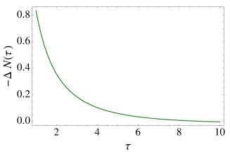
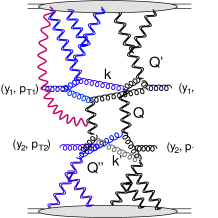
Fig. 3-a		Fig. 3-b

Figure 3: Fig. 3-a:$-\Delta N\left(\tau\right)=-4\,\tau\frac{1}{\tau}\frac{d}{d\tau}\tau\frac{d}{d\tau}N\left(\tau\right)$ versus $\tau$ for the behavior of the scattering amplitude deep in the saturation domainLETU . Fig. 3-b shows the example of a more complicated structure of the partonic cascades than the exchange of the BFKL Pomeron, which are shown in Fig. 2. The colour of the lines indicates the parton shower.

This approach is not correct for $\tau\to 1$ and $-\nabla^{2}N=1.58$ at $\tau=1$, but it starts to be small at $\tau>2$, which could be large enough to trust the formulae of Ref.LETU . At least such a conclusion can be justified considering the fit of the DIS data in the saturation model of Refs.CLP ; CLP1 , which based on the idea of Ref.IIM , and has the correct behavior of the scattering amplitude, both deep in the saturation domain, and near $\tau=1$. Hence, we expect that $\nabla^{2}N$ decreases faster than we can see from Eq. (5.47). Bearing these conclusions in mind, we will calculated the contribution of Fig. 2, keeping all $N$ in Eq. (5.36) in the vicinities of the saturation scales, by replacing $\int^{\infty}_{0}d\tau(-\nabla^{2}N)=-\int^{1}_{0}d\tau(-\nabla^{2}N)$.

We will show in the folowing, that we cannot take all six Pomerons in the vicinities of the saturation scale. We have to take two of them, either deep in the saturation domain, or in the perturbative QCD region. We choose to take two Pomerons between rapidities $y_{1}$ and $y_{2}$, (see Fig. 3-b) i.e. in the perturbative QCD region. Unfortunately, we cannot use the AGK cutting rulesAGK , which state that these Pomerons will be not affected by the Pomeron interaction, and the contributions of these interactions (see red Pomeron in Fig. 3-b) are canceled. Indeed, it has been proven that for the double inclusive productionKOJA , that they do not work in perturbative QCD. On the other hand, these Pomerons carry transverse momentum $Q_{T}$ , unlike the others one in the diagram, which is larger than the saturation scale $Q_{s}\left(y_{2}\right)$ and therefore, their contributions are suppressed in comparison with the other Pomerons in Fig. 2. In addition our choice provides the natural matching with the region $\bar{\alpha}_{S}\,y_{12}\,<\,1$.

The integration over $Q_{T}$ will produce the same result as Eq. (5.35), as in the previous section. We re-write the integration over $\phi_{i}$ (see Eq. (5.37)) in the following way:

$$\int\prod d\phi_{i}\,e^{-i\,\vec{p}_{T1}\cdot\vec{\tilde{r}}^{\prime}_{1}}\delta^{(2)}\left(\vec{r}_{1}+\vec{r}^{\prime}_{1}-\vec{\tilde{r}}_{1}-\vec{\tilde{r}}^{\prime}_{1}\right)\,\to\,\left(2\pi\right)^{4}\int d\phi\,e^{i\vec{p}_{T1}\cdot\vec{r}}\int k_{T}dk_{T}\,J_{0}\left(k_{T}r\right)\,J_{0}\left(k_{T}r_{1}\right)\,J_{0}\left(k_{T}\tilde{r}_{1}\right)\,J_{0}\left(k_{T}\tilde{r}^{\prime}_{1}\right)$$ (5.49)

We see that the integrals over $r^{\prime}_{1}$ and $r^{\prime}_{1}$ leads to $r_{1}\sim 1/Q_{s}(Y-y_{1})$ and $r^{\prime}_{1}\sim 1/Q_{s}(Y-y_{1})$. The same holds for the integrals over $r^{\prime}_{2}$ and $r^{\prime}_{2},$ leading to $r_{2}\sim 1/Q_{s}(y_{2})$ and $r^{\prime}_{2}\sim 1/Q_{s}(y_{2})$ . Assuming that $Q_{s}\left(Y-y_{1}\right)\,>\,Q_{s}\left(y_{2}\right)$ we conclude that $r_{i}$ and $r^{\prime}_{i}$ are much smaller than $r_{2}$ and $r^{\prime}_{2}$. Replacing

$$\nabla^{2}_{r_{1}}N_{\rm pr}\left(r_{1};Y-y_{1}\right)\,e^{i\vec{Q}_{T}\cdot\vec{\tilde{r}^{\prime}}_{1}}\,\nabla^{2}_{\tilde{r}^{\prime}_{1}}N_{\rm pr}\left(\tilde{r}^{\prime}_{1};Y-y_{1}\right)\,\to\,\frac{2^{8}\,\bar{\gamma}^{4}}{r_{1}\,r^{\prime}_{1}}\left(r^{2}_{1}\,Q^{2}_{s}\left(Y-y_{1}\right)\right)^{\bar{\gamma}}\left(r^{\prime 2}_{1}\,Q^{2}_{s}\left(Y-y_{1}\right)\right)^{\bar{\gamma}}$$ (5.50)

where $\bar{\gamma}=1-\gamma_{cr}$, we obtain from Eq. (5.49) that integration over $r$ takes the form

$$\frac{1}{Q_{s}}\frac{1}{1+2\bar{\gamma}}\,\int^{1}_{0}d\tau\,J_{0}\left(\frac{k_{T}}{Q_{s}}\sqrt{\tau}\right)\,\tau^{\bar{\gamma}}\frac{d\tau}{2\sqrt{\tau}}\,=\,\frac{1}{Q_{s}}\frac{1}{1+2\bar{\gamma}}\,{}_{1}F_{2}\left(\{\frac{1}{2}+\bar{\gamma}\},\{1,\frac{3}{2}+\bar{\gamma}\},-\frac{k^{2}_{T}}{4\,Q^{2}_{s}}\right)$$ (5.51)

Recall that we consider $Q_{s}=Q_{s}(Y-Y_{1})$ in Eq. (5.51). For $p_{T1}\ll\,Q_{s}\left(Y-y_{1}\right)$ we can replace $e^{-i\,\vec{p}_{T1}\cdot\vec{\tilde{r}}^{\prime}_{1}}\,=\,1$ in Eq. (5.49). In this case the integral has the form

$$\frac{1}{Q^{2}_{s}}\frac{1}{(1+2\bar{\gamma})^{2}}\,\int^{1}_{0}d\tau^{\prime}\,\Bigg{(}\frac{1}{Q_{s}}\frac{1}{1+2\bar{\gamma}}\,{}_{1}F_{2}\left(\{\frac{1}{2}+\bar{\gamma}\},\{1,\frac{3}{2}+\bar{\gamma}\},-\frac{1}{4\,\tau^{\prime}}\right)\Bigg{)}^{2}\frac{d\tau^{\prime}}{\tau^{\prime}}\,=\,0.18/Q^{2}_{s}$$ (5.52)

where $\tau^{\prime}=k^{2}/Q^{2}_{s}$.

The integral over $r$ in the lower part of the diagram takes the form:

$$\int\frac{d^{2}r^{\prime}}{r^{\prime 2}}\,J_{0}\left(k_{T}\,r\right)\,=\,\pi\,\ln\left(k^{2}_{T}/(4\mu^{2}_{\rm soft})\right)$$ (5.53)

Using Eq. (5.53) for $p_{T2}\ll Q_{s}\left(y_{2}\right)$ the integral over $k^{\prime}_{T}$ can be reduced to

$$\frac{1}{(1+2\bar{\gamma})^{2}}\,\int^{1}_{0}d\tau^{\prime\prime}\,\Bigg{(}\,{}_{1}F_{2}\left(\{\frac{1}{2}+\bar{\gamma}\},\{1,\frac{3}{2}+\bar{\gamma}\},-\frac{1}{4\,\tau^{\prime\prime}}\right)\Bigg{)}^{2}\,\left(\frac{\ln\left(\tau^{\prime\prime}\right)}{\tau^{\prime\prime}}\right)^{2}\,=\,3.50$$ (5.54)

Finally, collecting all numerical coefficients, we obtain

$$\frac{d^{2}\sigma}{dy_{1}d^{2}p_{T1}\,dy_{2}d^{2}p_{T2}}\left({Fig.~{}\ref{DN}}-b\right)\,\,=$$ (5.55)

$$\,\,\mbox{C}^{4}\,2^{3}\pi^{3}\left(\frac{2C_{F}}{\alpha_{S}\,(2\pi)^{2}}\right)^{2}\,\,\frac{1}{p^{2}_{T1}\,p^{2}_{T2}}\frac{0.18\,3.5}{Q^{2}_{s}\left(Y-y_{1}\right)}\left(2\bar{\gamma}\right)^{8}\,\sqrt{\frac{1}{\left(2\,D\,y_{12}\right)^{3}}}\,\,e^{2\Delta_{\rm BFKL}\,y_{12}}\,$$

where constant C is the value of the amplitude at $\tau=1$.

This contribution is proportional to

$$\propto~{}~{}~{}e^{2\Delta_{\rm BFKL}\,y_{12}}\Big{/}Q^{2}_{s}\left(Y-y_{1}\right)$$

for $p_{T1}\ll Q_{s}\left(Y-y_{1}\right)$ and $p_{T2}\ll Q_{s}\left(y_{2}\right)$. Note that $Q^{2}_{s}\left(Y-y_{1}\right)\,>\,Q^{2}_{s}\left(y_{2}\right)$.

We need to estimate the diagram of Fig. 1-a (see Eq. (2)). This diagram can be re-written as

$$\frac{d^{2}\sigma}{dy_{1}d^{2}p_{T1}\,dy_{2}d^{2}p_{T2}}\left({Fig.~{}\ref{becor}}-a\right)\,\, = \,\,\tilde{\mu}^{2}_{\rm soft}\frac{d^{2}\sigma}{dy_{1}d^{2}p_{T1}}\left(Q_{T}=0;{Eq.~{}(\ref{SINCL3})}\right)\,\frac{d^{2}\sigma}{dy_{2}d^{2}p_{T2}}\left(Q_{T}=0;{Eq.~{}(\ref{SINCL3})}\right)$$ (5.56)

where $$~{}~{}~{}~{}\tilde{\mu}^{2}_{\rm soft}\,=\,\int d^{2}Q_{T}\,N^{2}\left(Q_{T}\right);$$

Examining Eq. (4.21), one can see that in general case when $Y-y_{1}\neq y_{1}$ and $Y-y_{2}\neq y_{2}$ all four Pomerons cannot be in the vicinity of the saturation scale. Actually we have two kinematic regions which give the maximal contributions (assuming $Q_{s}\left(Y-y_{1}\right)\,>\,Q^{2}_{s}\left(y_{1}\right)$):

1. $r^{2}\,Q^{2}_{s}\left(Y-y_{1}\right)\,\approx\,1$ but $r^{2}Q^{2}_{s}\left(y_{1}\right)\to Q^{2}_{s}\left(Y-y_{1}\right)\Big{/}Q^{2}_{s}\left(y_{1}\right)\,\ll\,1$;

2. $r^{2}\,Q^{2}_{s}\left(y_{1}\right)\,\approx\,1$ but $r^{2}Q^{2}_{s}\left(y_{1}\right)\to Q^{2}_{s}\left(y_{1}\right)\Big{/}Q^{2}_{s}\left(Y-y_{1}\right)\,\gg\,1$;

In the region 1 the upper Pomeron is in the vicinity of the saturation scale, while the lower Pomeron is in the perturbative QCD region. In region 2 the lower Pomeron is in the vicinity of the saturation scale, and the upper Pomeron is deep inside the saturation domain. As we have discussed (see Fig. 3-a) $\nabla^{2}N$ decreases in the saturation region much faster than in the perturbation QCD region and, therefore, we bf assume that the kinematic region 1 gives the largest contribution. Hence, for $p_{T1}\,\ll\,Q^{2}_{s}\left(y_{1}\right)$ we obtain

$$\frac{d^{2}\sigma}{dy_{1}d^{2}p_{T1}}\left(Q_{T}=0;{Eq.~{}(\ref{SINCL3})}\right)=$$

$$\,\,\frac{8C_{F}}{\alpha_{S}\,(2\pi)^{2}}\frac{1}{p^{2}_{T}}\int d^{2}r\,e^{i\vec{p}_{T}\cdot\vec{r}}\,\nabla^{2}_{r}\,N^{\rm\tiny BFKL}_{\rm pr}\,\left(r,r_{1};Y-y,Q_{T}=0\right)\,\nabla^{2}_{r}\,N^{\rm\tiny BFKL}_{\rm tr}\,\left(r,r_{2};y,Q_{T}=0\right)$$

$$=\,\,\frac{8C_{F}}{\alpha_{S}\,(2\pi)^{2}}\frac{1}{p^{2}_{T}}\mbox{C}^{2}\,(4\bar{\gamma}^{2})^{2}\,\exp\left(-\frac{\ln^{2}\left(Q^{2}_{s}\left(Y-y\right)/Q^{2}\left(y\right)\right)}{4D\,y}\right)$$ (5.57)

In Eq. (5.2) we used backward evolution, from the saturation boundary where $N=\mbox{C}$.

The ratio of two contributions takes the following form:

$$R\,=\,\frac{\frac{d^{2}\sigma}{dy_{1}d^{2}p_{T1}\,dy_{2}d^{2}p_{T2}}\left({Fig.~{}\ref{DN}}-b\right)}{\frac{d^{2}\sigma}{dy_{1}d^{2}p_{T1}\,dy_{2}d^{2}p_{T2}}\left({Fig.~{}\ref{becor}}-a\right)}\,=\,\frac{1}{N^{2}_{c}-1}\frac{\tilde{\mu}^{2}_{\rm soft}}{Q^{2}_{s}\left(y_{2}\right)}\,8\,\pi^{5}\,\left(2\,\bar{\gamma}\right)^{4}\,\,0.18\,\,3.5$$ (5.58)

$$\times\,\,\,\sqrt{\frac{\pi}{\left(2\,D\,y_{12}\right)^{3}}}\,\,e^{2\Delta_{\rm BFKL}\,y_{12}}\,\,\exp\left(\frac{\ln^{2}\left(Q^{2}_{s}\left(Y-y_{1}\right)/Q^{2}\left(y_{1}\right)\right)}{4D\,y_{1}}\right)\exp\left(\frac{\ln^{2}\left(Q^{2}_{s}\left(Y-y_{2}\right)/Q^{2}\left(y_{2}\right)\right)}{4D\,y_{2}}\right)$$

One can see that Eq. (5.58) demonstrates the additional suppression in comparison with the calculation of the simplest diagram, due to infrared cutoff at $Q_{s}\left(y_{2}\right)$ instead of $p_{T2}$. The factor $\exp\left(2\Delta_{\rm BFKL}\,y_{12}\right)$ reflects the fact that two BFKL Pomerons between rapidities $y_{1}$ and $y_{2}$ are taken in the perturbative QCD region. It should be stressed that we can trust our estimates only for values of $y_{12}$ at which the exchange of the BFKL Pomeron with rapidity $y_{12}$ give the contribution smaller than ${\rm C}$. This condition means that

$$\frac{1}{\left(2\,D\,y_{12}\right)}\,\,e^{2\Delta_{\rm BFKL}\,y_{12}}\,\,<\,\,{\rm C}$$ (5.59)

Taking $\Delta_{\rm BFKL}=0.25$ and $Q^{2}_{s}(Y)\propto\exp\left(\lambda Y\right)$ with $\lambda=0.25$ (these values correspond to the BFKL phenomenology) we obtain that the l.h.s. of Eq. (5.59) is smaller than 0.15 for $y_{12}\,\leq\,7$. Therefore, we can trust our estimates shown in Fig. 4 for ${\rm C}\,>\,0.15$. We are used to take ${\rm C}=0.3$ which lead to the contribution of the shadowing corrections of the order of 30%.

Two last factors in Eq. (5.58) stem from the perturbative QCD nature of two Pomerons in Eq. (5.56) ( see Eq. (5.2)).

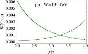
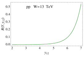
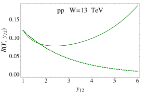
Fig. 4-a	Fig. 4-b	Fig. 4-c

Figure 4: The ratio of Eq. (5.58) at W=13 TeV versus $y_{12}$, assuming that the experiment has a symmetric pattern with $Y-y_{1}=y_{2}=\frac{1}{2}(Y-y_{12})$. The dotted line in Fig. 4-a is the estimates for the $y_{12}$ dependence of the Bose-Einstein contribution at small $y_{12}$ GLMBEH ; GOLELAST . Fig. 4-a and Fig. 4-b give the estimates in the leading order of perturbative QCD with $\bar{\alpha}_{S}=0.25$. In Fig. 4-c we take $\Delta_{\rm BFKL}=0.25$ and $Q^{2}_{s}(Y)\propto\exp\left(\lambda Y\right)$ with $\lambda=0.25$. These numbers correspond to the BFKL phenomenology.

In Fig. 4 we plotted ratio $R$ as function of $y_{12}$ for $y_{12}\leq 7$ (see Eq. (5.59). One can see that the ratio increases for large $y_{12}$ .

6 Azimuthal angle correlations

The azimuthal angle correlations stem from terms $\left(\vec{Q}_{T}\cdot\vec{r}_{i}\right)^{n}$ in the vertices (see Eq. (3.12) and Eq. (3.13)). Indeed, after integrating over $r_{i}$ these terms transform to expressions of the following typeLERECOR :
$\left(\vec{Q}_{T}\cdot\vec{p}_{T1}\right)^{m_{1}}\,\left(\vec{Q}_{T}\cdot\vec{p}_{T2}\right)^{m_{2}}$, which lead to term of $\left(\vec{p}_{T1}\cdot\vec{p}_{T2}\right)^{m}$. We have illustrated in Eq. (3.12) and Eq. (3.13) how these originate from the general form of BFKL the Pomeron vertices in the coordinate representation. From Eq. (3.12) and Eq. (3.13) only terms proportional to $\left(\vec{Q}_{T}\cdot\vec{r}_{i}\right)^{n}$ with even $n$ appear in the expansion. Therefore, the azimuthal angle ($\phi$) correlation function contains only terms $\cos^{2n}\left(\phi\right)$, and it is invariant with respect to $\phi\to\pi-\phi$. In other words, $v_{n}$ with odd $n$, turn out to be zero. Hence, we have the first prediction: the value $v_{n}$ with odd $n$ should decreases with $y_{12}$, and their dependence should follow the dotted lines in Fig. 4-a.

We return to Eq. (5.29) and integrate over $Q_{T}$, collecting terms that depend on the angles between $\vec{Q}_{T}$ and $\vec{r}_{i}$, which we have neglected in the previous section. As we have learned the typical values of $Q_{T}\propto 1/r_{2}\sim 1/r^{\prime}_{2}$ where $r_{2}$ and $r^{\prime}_{2}$ are larger than $r_{1}$ and $r^{\prime}_{1}$. In other words , we showed that the main contributions stem from the kinematic regions: $r^{2}_{1}Q^{2}_{s}\left(Y-y_{1}\right)\sim 1$ ( $r^{\prime 2}_{1}Q^{2}_{s}\left(Y-y_{1}\right)\sim 1$ ) and $r^{2}_{2}Q^{2}_{s}\left(y_{2}\right)\sim 1$ ( $r^{\prime 2}_{2}Q^{2}_{s}\left(y_{2}\right)\sim 1$ ). Assuming that $Q_{s}\left(Y-y_{1}\right)\gg Q_{s}\left(y_{2}\right)$ we conclude that $r_{1}(r^{\prime}_{1})\ll r_{2}(r^{\prime}_{2})$. The typical $Q_{T}$ is determined by the largest dipoles and, therefore, we expect $Q_{T}\approx 1/r_{2}(1/r^{\prime}_{2})$, as has been demonstrated above. Bearing these estimate in mind, we can replace vertices $V_{\nu_{1}}\left(\vec{r}_{1},\vec{Q}_{T}\right)$ and $V_{\nu_{2}}\left(\vec{r}^{\prime}_{1},\vec{Q}_{T}\right)$ in Eq. (5.29) by Eq. (3.13) in which we put $Q_{T}=1/r_{2}$ and $Q_{T}=1/r^{\prime}_{2}$, respectively. Taking into account that $r_{1}/r_{2}\,\ll\,1(r^{\prime}_{1}/r^{\prime}_{2}\,\ll\,1)$ we obtain

$$V_{\nu_{1}}\left(\vec{r}_{1},\vec{Q}_{T}\right)\,V_{\nu_{2}}\left(\vec{r}^{\prime}_{1},\vec{Q}_{T}\right) =$$

$$\Bigg{\{}\left(\frac{r^{2}_{1}}{2^{6}}\right)^{-i\nu_{1}}-\left(\frac{Q^{4}_{T}r^{2}_{1}}{2^{6}}\right)^{i\nu_{1}}\Bigg{\}}\,\left(1\,-\,\frac{1}{2^{4}}\left(\vec{Q}_{T}\cdot\vec{r}_{1}\right)^{2}\,+\,\frac{1}{2^{8}}\left(\vec{Q}_{T}\cdot\vec{r}_{1}\right)^{4}\right)$$

$$\times \,\Bigg{\{}\left(\frac{r^{\prime 2}}{2^{6}}\right)^{-i\nu_{2}}-\left(\frac{Q^{4}_{T}r^{\prime 2}_{1}}{2^{6}}\right)^{i\nu_{2}}\Bigg{\}}\,\left(1\,-\,\frac{1}{2^{4}}\left(\vec{Q}_{T}\cdot\vec{r}^{\prime}_{1}\right)^{2}\,+\,\frac{1}{2^{8}}\left(\vec{Q}_{T}\cdot\vec{r}^{\prime}_{1}\right)^{4}\right)$$

At first sight Eq. (6) should enter two angles between $\vec{Q}_{T}$ and $\vec{r}_{1}$ and $\vec{r}^{\prime}_{1}$, respectively. However, in the integrand for integration over $r_{i}$ (see Eq. (5.37)) depends only on one vector $\vec{p}_{T1}$ . Therefore, after integration over all angles, we find that the angle $\phi$ in Eq. (6) is the angle between $\vec{Q}_{T}$ and $\vec{p}_{T1}$.

For vertices $V^{*}_{\nu_{1}}\left(\vec{r}_{2},\vec{Q}_{T}\right)$ and $V^{*}_{\nu_{2}}\left(\vec{r}^{\prime}_{2},\vec{Q}_{T}\right)$ in Eq. (5.29) we use Eq. (3.15). Finally, we need to evaluate the integral

$$I_{Q}\,=$$ (6.61)

$$\,-16\,\nu_{1}\,\nu_{2}\int Q_{T}dQ_{T}\Bigg{\{}V_{\nu_{1}}\left(\vec{r}_{1},\vec{Q}_{T}\right)\,V_{\nu_{2}}\left(\vec{r}^{\prime}_{1},\vec{Q}_{T}\right)\Bigg{\}}^{r_{1}\,=\,r^{\prime}_{1}=1/Q_{s}\left(Y-y_{1}\right)}_{{Eq.~{}(\ref{ANGLECOR1})}}\!\!\!\!\!\!\!\!\!\!\!\!\!\!\!\!\!\!\!\!\!\!\!\!\left(Q^{2}_{T}\right)^{-i(\nu_{1}+\nu_{2})}\frac{\cos^{2}\left(\frac{1}{2}\vec{Q}_{T}\cdot\vec{r}_{2}\right)}{Q^{2}_{T}\,r^{2}_{2}}\,\cos\left(\vec{Q}_{T}\cdot\vec{r}_{2}\right)$$

with better accuracy that we did in section 5.1, keeping the dependence on the angle between $\vec{Q}_{T}$ and $\vec{r}_{2}$. Note, that the factor $\cos\left(\vec{Q}_{T}\cdot\vec{r}_{2}\right)$ comes from $\exp\left(i\,\vec{Q}_{T}\cdot\vec{r}_{2}\right)$ in Eq. (5.36). Taking this integral we substitute for the terms in parentheses in Eq. (6), $|Q_{T}|=1/r^{2}_{2}(1/r^{\prime 2}_{2})$.

The integral is equal to

$$I_{Q} = 2^{6i(\nu_{1}+\nu_{2})}\left(-2^{7}\nu_{1}\,\nu_{2}\right)\ \left(\frac{r^{2}_{1}}{r^{2}_{2}}\right)^{i\,(\nu_{1}+\nu_{2})}\frac{1}{r^{2}_{2}}$$

$$\times \,\left(1\,-\,\frac{1}{2^{4}}\frac{\left(\vec{n}\cdot\vec{r}_{1}\right)^{2}}{r^{2}_{2}}\,+\,\frac{1}{2^{8}}\frac{\left(\vec{n}\cdot\vec{r}_{1}\right)^{4}}{r^{4}_{2}}\right)\,\left(1\,-\,\frac{1}{2^{4}}\frac{\left(\vec{n}\cdot\vec{r}^{\prime}_{1}\right)^{2}}{r^{\prime 2}_{2}}\,+\,\frac{1}{2^{8}}\frac{\left(\vec{n}\cdot\vec{r}^{\prime}_{1}\right)^{4}}{r^{\prime 4}_{2}}\right)$$

$$\times \Bigg{\{}\frac{1}{i(\nu_{1}+\nu_{2})}\,-\,\frac{9}{32}\,\cos\left(2\phi_{2}\right)\,+\,\frac{3}{16}\cos\left(4\,\phi_{2}\right)\Bigg{\}}$$

where $\vec{n}=\vec{Q}_{T}/Q_{T}$, and $\phi_{2}$ is the angle between $\vec{n}$ and $\vec{n}_{2}=\vec{r}_{2}/r_{2}$. In Eq. (6) the terms in $\left(\dots\right)\left(\dots\right)$ stem from the expansion with respect to $r^{2}_{1}/r^{2}_{2}\,\ll\,1$. However, for the terms in $\{\dots\}$ there are no such small parameters, and we expand the function of $\phi_{2}$ in the Fourier series.

Integrating over $\vec{n}$ one obtains

$$\left(\dots\right)\left(\dots\right)\left\{\dots\right\}\,=\,\frac{1}{i(\nu_{1}+\nu_{2})}\,+\,\frac{3}{2^{10}}\frac{r^{2}_{1}}{r^{2}_{2}}\left(\left(\vec{n}_{1}\cdot\vec{n}_{2}\right)^{2}\,+\left(\vec{n}^{\prime}_{1}\cdot\vec{n}_{2}\right)^{2}\right)\,+\,\frac{3}{2^{12}}\frac{r^{4}_{1}}{r^{4}_{2}}\left(\left(\vec{n}_{1}\cdot\vec{n}_{2}\right)^{4}\,+\,\left(\vec{n}^{\prime}_{1}\cdot\vec{n}_{2}\right)^{4}\right)$$ (6.63)

where $\vec{n}_{1}=\vec{r}_{1}/r_{1},\vec{n}^{\prime}_{1}=\vec{r}_{1}/r_{1}$ and $\vec{n}_{2}=\vec{r}_{2}/r_{2}$. Deriving Eq. (6.63) we neglected the extra powers of $r^{2}_{1}/r^{2}_{2}$ , which are small. Finally

$$I_{Q}\left(\vec{r}_{1},\vec{r}^{\prime},\vec{r}_{2};\nu_{1},\nu_{2}\right) = 2^{6i(\nu_{1}+\nu_{2})}\left(-2^{7}\nu_{1}\,\nu_{2}\right)\ \left(\frac{r^{2}_{1}}{r^{2}_{2}}\right)^{i\,(\nu_{1}+\nu_{2})}\frac{1}{r^{2}_{2}}$$

$$\times \Bigg{\{}\frac{1}{i(\nu_{1}+\nu_{2})}\,+\,\frac{9}{2^{10}}\frac{r^{2}_{1}}{r^{2}_{2}}\left(\left(\vec{n}_{1}\cdot\vec{n}_{2}\right)^{2}\,+\left(\vec{n}^{\prime}_{1}\cdot\vec{n}_{2}\right)^{2}\right)\,+\,\frac{3}{2^{12}}\frac{r^{4}_{1}}{r^{4}_{2}}\left(\left(\vec{n}_{1}\cdot\vec{n}_{2}\right)^{4}\,+\,\left(\vec{n}^{\prime}_{1}\cdot\vec{n}_{2}\right)^{4}\right)\Bigg{\}}$$

From Eq. (5.36) we can see that the integration over $r_{i}$ can be written in the form

$$\frac{d^{2}\sigma}{dy_{1}d^{2}p_{T1}\,dy_{2}d^{2}p_{T2}}\left({Fig.~{}\ref{mudia}}\right)\,\,=\,\,\left(\frac{2C_{F}\,\mu^{2}_{\rm soft}}{\alpha_{S}\,(2\pi)^{2}}\right)^{2}\,\,\frac{1}{p^{2}_{T1}\,p^{2}_{T2}}\,$$ (6.65)

$$\times\,\,\int d^{2}r_{1}\,d^{2}r^{\prime}_{1}\,d^{2}\tilde{r}_{1}\,d^{2}\tilde{r}^{\prime}_{1}\,e^{-i\,\vec{p}_{T1}\cdot\vec{{r}}_{1}}\delta^{(2)}\left(\vec{r}_{1}+\vec{r}^{\prime}_{1}-\vec{\tilde{r}}_{1}-\vec{\tilde{r}}^{\prime}_{1}\right)\,\nabla^{2}_{\tilde{r}_{1}}\tilde{r}_{1}V_{\rm pr}\left(\tilde{r}_{1}\right)\,\,\nabla^{2}_{\tilde{r}^{\prime}_{1}}\tilde{r}^{\prime}_{1}V_{\rm pr}\left(\tilde{r}^{\prime}_{1}\right)$$

$$\times\,\int d^{2}r_{2}\,d^{2}r^{\prime}_{2}\,d^{2}\tilde{r}_{2}\,d^{2}\tilde{r}^{\prime}_{2}\,e^{-i\,\vec{p}_{T2}\cdot\vec{{r}}_{2}}\delta^{(2)}\left(\vec{r}_{2}+\vec{r}^{\prime}_{2}-\vec{\tilde{r}}_{2}-\vec{\tilde{r}}^{\prime}_{2}\right)\,\nabla^{2}_{\tilde{r}_{2}}r_{2}V_{\rm tr}\left(\tilde{r}_{2}\right)\,\,\nabla^{2}_{\tilde{r}^{\prime}_{2}}\tilde{r}^{\prime}_{2}V_{\rm tr}\left(\tilde{r}^{\prime}_{2}\right)$$

$$\times\,\,\nabla^{2}_{{r}_{1}}\nabla^{2}_{{r}_{2}}\nabla^{2}_{{r}^{\prime}_{1}}\nabla^{2}_{{r}^{\prime}_{2}}\,\Bigg{(}{r}_{1}\,{r}_{2}\,{r}^{\prime}_{1}\,{r}^{\prime}_{2}\,I_{Q}\left(\vec{r}_{1},\vec{r}^{\prime},\vec{r}_{2};\nu_{1},\nu_{2}\right)\Bigg{)}$$

$$\times\,2\pi\Bigg{\{}\frac{1}{i(\nu_{1}+\nu_{2})}\,+\,\,\frac{9}{2^{10}}\frac{r^{2}_{1}}{r^{2}_{2}}\left(\left(\vec{n}_{1}\cdot\vec{n}_{2}\right)^{2}\,+\left(\vec{n}^{\prime}_{1}\cdot\vec{n}_{2}\right)^{2}\right)\,+\,\frac{3}{2^{12}}\frac{r^{4}_{1}}{r^{4}_{2}}\left(\left(\vec{n}_{1}\cdot\vec{n}_{2}\right)^{4}\,+\,\left(\vec{n}^{\prime}_{1}\cdot\vec{n}_{2}\right)^{4}\right)\Bigg{\}}$$

Each term in Eq. (6.65) can be factorized as a product of two functions which depend on $r^{i}_{1}$ and on $r^{i}_{2}$. Bearing this feature in mind we calculate each term going to the momentum representation using Eq. (5.49). We obtain a product of functions of $k_{T}$. Each of these function has the following general form:

$$\int d^{2}r\,e^{i\vec{k}_{T}\cdot\vec{r}}\,\prod_{i=1}^{j}\,r_{\mu_{i}}\,F\left(r\right)\,\,=\,\,(-i\vec{\nabla}_{k_{T}})^{j}\,\int d^{2}r\,e^{i\vec{k}_{T}\cdot\vec{r}}\,\,F\left(r\right)\,\,=\,\,2\pi\,(-i\vec{\nabla}_{k_{T}})^{j}\,\int d^{2}r\,J_{0}\left(k_{T}\,r\right)\,\,F\left(r\right)$$ (6.66)

As we have seen the dependence on $\vec{r}_{i}$ stem from the integration over $Q_{T}$ or, in other words, from $I_{Q}$ In $I_{Q}$ dependence on $r_{1}$ and $r^{\prime}_{1}$ can be extracted explicitly, leading to $F\left(r\right)\propto 1/r$. Hence the momentum image for Eq. (6.66) has a simple form:

$$\int d^{2}r\,e^{i\vec{k}_{T}\cdot\vec{r}}\,\prod_{i=1}^{j}\,r_{\mu_{i}}\,F\left(r\right)\,\,=\,\,\,2\pi\,(-i\vec{\nabla}_{k_{T}})^{j}\frac{1}{k_{T}}$$ (6.67)

For $j=2$ and $j=4$ which we need to calculate Eq. (6.65) we have

$$(-i\vec{\nabla}_{k_{T}})^{2}\frac{1}{k_{T}}\,=\,\Big{\{}\frac{3}{k^{5}_{T}}\,k_{T,i}\,k_{T,i^{\prime}}\,-\,\frac{1}{k^{3}_{T}}\delta_{i,i^{\prime}}\Big{\}};$$

$$(-i\vec{\nabla}_{k_{T}})^{4}\frac{1}{k_{T}}\,=\,\Big{\{}\frac{105}{k^{9}_{T}}\,k_{T,i}\,k_{T,i^{\prime}}\,k_{T,j}\,k_{T,j^{\prime}}$$

$$\,-\,\frac{15}{k^{7}_{T}}\left(\delta_{ij}\,k_{T,i^{\prime}}\,k_{T,j^{\prime}}\,+\,\delta_{ii^{\prime}}\,k_{T,j}\,k_{T,j^{\prime}}\,+\,\delta_{i^{\prime}j}\,k_{T,i}\,k_{T,j^{\prime}}\,+\,\delta_{ji^{\prime}}\,k_{T,i}\,k_{T,j^{\prime}}\,+\,\delta_{i^{\prime}j^{\prime}}\,k_{T,j}\,k_{T,i}\,+\,\delta_{jj^{\prime}}\,k_{T,i}\,k_{T,i^{\prime}}\right)\,$$

$$+\,\frac{3}{k^{5}}\left(\delta_{ii^{\prime}}\delta_{jj^{\prime}}\,+\,\delta_{ij}\delta_{i^{\prime}j^{\prime}}\,+\,\delta_{ij}\delta_{i^{\prime}j^{\prime}}\right)\Big{\}};$$

Note that for integration over $\vec{r}_{1}$, Eq. (6.67) takes the form

$$\int d^{2}r_{1}\,e^{i(\vec{k}_{T}+\vec{p}_{T1})\cdot\vec{r}_{1}}\,\prod_{i=1}^{j}\,r_{1,\mu_{i}}\,F\left(r_{1}\right)\,\,=\,\,\,2\pi\,(-i\vec{\nabla}_{\vec{k}_{T}+\vec{p}_{T1}})^{j}\frac{1}{\sqrt{(\vec{k}_{T}\,+\,\vec{p}_{T1})^{2}}}$$ (6.68)

The term $\left(r^{2}_{1}\left(\vec{n}_{1}\cdot\vec{n}_{2}\right)^{2}\,+r^{\prime 2}_{1}\left(\vec{n}^{\prime}_{1}\cdot\vec{n}_{2}\right)^{2}\right)$ can be re-written as $\left(r_{1,\mu}\,r_{1,\nu}\,+\,r^{\prime}_{1,\mu}\,r^{\prime}_{1,\nu}\right)r_{2,\mu}\,r_{2,\nu}$ and in the momentum representation it looks as

$$\int d\phi\Bigg{\{}\Big{(}\frac{3}{k^{5}_{T}}\,k_{T,i}\,k_{T,i^{\prime}}\,-\,\frac{\delta_{ii^{\prime}}}{k^{3}_{T}}\Big{)}\frac{1}{\sqrt{k^{2}_{T}+p^{2}_{T1}+2\cos\left(\phi\right)k_{T}p_{T1}}}\,+$$ (6.69)

$$\,\Big{(}\frac{3}{\left(\sqrt{k^{2}_{T}+p^{2}_{T1}+2\cos\left(\phi\right)k_{T}p_{T1}}\right)^{5}}\,(\vec{k}_{T}+\vec{p}_{T1})_{i}\,(\vec{k}_{T}+\vec{p}_{T1})_{i^{\prime}}\,-\,\frac{\delta_{ii^{\prime}}}{\left(\sqrt{k^{2}_{T}+p^{2}_{T1}+2\cos\left(\phi\right)k_{T}p_{T1}}\right)^{3}}\Big{)}\frac{1}{k_{T}}\Bigg{\}}$$

$$=\,\,A\,\frac{p_{T1,i}\,p_{T1,i^{\prime}}}{p^{2}_{T1}}\,+\,B\,\,\delta_{ii^{\prime}}$$

The expressions for $A$ and $B$ can be written in a general form. Assuming that both $p_{T1}$ and $p_{T2}$ are smaller than $Q_{s}\left(y_{2}\right)$, we can expand the answer, only taking into account terms that are proportional to $p^{2}_{T1}/k^{2}_{T}$ and $p_{T2}^{2}/k^{\prime 2}_{T}$. We obtain

$$A\left(k_{T},p_{T1}\right)\,=\,\frac{3p^{2}_{T1}}{4\,k^{8}_{T}}\left(-13k^{2}_{T}\,+\,50\,p^{2}_{T1}\right);~{}~{}~{}~{}~{}~{}~{}~{}~{}~{}~{}B\left(k_{T},p_{T1}\right)\,=\,\frac{1}{8\,k^{4}_{T}}\left(8k^{4}_{T}+65k^{2}_{T}p^{2}_{T1}-150p^{4}_{T1}\right);$$ (6.70)

The integrations over $r^{\prime}_{2}$ and $r_{2}$ differ from the integrations over $r_{1}$ and $r^{\prime}_{1}$, due to extra factor $1/r^{2}_{2}$ which comes from the integration over $Q_{T}$ in Eq. (5.30) and Eq. (5.31). Since $r^{2}_{2}\approx\,1/Q^{2}_{s}(y_{2})$ we replace it by $1/r^{2}_{2}=Q^{2}_{s}\left(y_{2}\right)$. In the case the integral over $k^{\prime}_{T}$ takes the same form as the integral over $k_{T}$, leading to the following expression which is proportional to $\cos^{2}\left(\phi\right)$, where $\phi$ is the bangle between $\vec{p}_{T1}$ and $\vec{p}_{T2}$:

$$\frac{d^{2}\sigma}{dy_{1}d^{2}p_{T1}\,dy_{2}d^{2}p_{T2}}\left({Fig.~{}\ref{mudia}}\right)\,\,\propto\,\,\,Q^{2}_{s}\left(y_{2}\right)\,\,A\left(k_{T},p_{T1}\right)\,A\left(k^{\prime}_{T},p_{T2}\right)\,\cos^{2}\left(\phi\right)$$ (6.71)

which is responsible for the appearance of $v_{2,2}$ and $v_{2}$.

Using the second expression in Eq. (6.70) we can calculate the term which is proportional to $\cos^{4}\left(\phi\right)$ and has the form

$$\frac{d^{2}\sigma}{dy_{1}d^{2}p_{T1}\,dy_{2}d^{2}p_{T2}}\left({Fig.~{}\ref{mudia}}\right)\,\,\propto\,\,\,Q^{2}_{s}\left(y_{2}\right)\,\,A^{(4)}\left(k_{T},p_{T1}\right)\,A^{(4)}\left(k^{\prime}_{T},p_{T2}\right)\,\cos^{4}\left(\phi\right)$$ (6.72)

with

$$A^{(4)}\left(k_{T},p_{T1}\right)\,\,=\,\,15\,\frac{573}{8}\frac{1}{k^{6}_{T}}\,\frac{p^{2}_{T1}}{k^{2}_{T}}$$ (6.73)

The values of $v_{2}$ and $v_{4}$ can be determined from the following representation of the double inclusive cross section

$$\frac{d^{2}\sigma}{dy_{1}\,dy_{2}d^{2}p_{T1}d^{2}p_{T2}}\,\,\propto\,\,1\,\,+\,\,2\sum_{n}v_{n,n}\left(p_{T1},p_{T2}\right)\,\cos\left(n\,\varphi\right)$$ (6.74)

where $\varphi$ is the angle between $\vec{p}_{T1}$ and $\vec{p}_{T2}$. $v_{n}$ is calculated from $v_{n,n}\left(p_{T1},p_{T2}\right)$

$$1.~{}~{}v_{n}\left(p_{T}\right)\,\,=\,\,\sqrt{v_{n,n}\left(p_{T},p_{T}\right)}\,;\,~{}~{}~{}~{}~{}~{}~{}~{}~{}~{}~{}~{}~{}2.~{}~{}~{}~{}v_{n}\left(p_{T}\right)\,\,=\,\,\frac{v_{n,n}\left(p_{T},p^{\rm Ref}_{T}\right)}{\sqrt{v_{n,n}\left(p^{\rm Ref}_{T},p^{\rm Ref}_{T}\right)}}\,;$$ (6.75)

Eq. (6.75)-1 and Eq. (6.75)-2 depict two methods of how the values of $v_{n}$ have been extracted from the experimentally measured $v_{n,n}\left(p_{T1},p_{T2}\right)$, where $p^{\rm Ref}_{T}$ denotes the momentum of the reference trigger. These two definitions are equivalent if $v_{n,n}\left(p_{T1},p_{T2}\right)$ can be factorized as $v_{n,n}\left(p_{T1},p_{T2}\right)\,=\,v_{n}\left(p_{T1}\right)\,v_{n}\left(p_{T2}\right)$. In this paper we use the definition in Eq. (6.75)-1.

Introducing the angular correlation function as

$$C\left(p_{T},\phi\right)\,\,\equiv\,\,\frac{\frac{d^{2}\sigma}{dy_{1}d^{2}p_{T1}\,dy_{2}d^{2}p_{T2}}\left({Fig.~{}\ref{DN}}-b\right)}{\frac{d^{2}\sigma}{dy_{1}d^{2}p_{T1}\,dy_{2}d^{2}p_{T2}}\left({Fig.~{}\ref{becor}}-a\right)}$$ (6.76)

we obtain

$$v_{n,n}\,\,=\,\,\frac{\int^{2\pi}_{0}d\phi\,C\Big{(}\,p_{T},\,\phi\Big{)}\,\cos\left(n\,\phi\right)}{2\,\pi\,+\,\int^{2\pi}_{0}d\phi\,C\Big{(}p_{T},\phi\Big{)}};~{}~{}~{}~{}~{}~{}v_{n}\,=\,\sqrt{v_{n,n}}\,;$$ (6.77)

In Eq. (5.58) we have calculated the part of $C\left(p_{T},\phi\right)$ which does not depend on $\phi$, which coincides with $C\left(p_{T},\phi=0\right)$ = $R$ of Eq. (5.58) for $Q_{s}\left(Y-y_{1}\right)\,\gg\,Q_{s}\left(y_{2}\right)$. To calculate the contribution to $C$, which depends on $\phi$, we need to take the separate integrals over $\nu_{1}$ and $\nu_{2}$ since the terms, which are proportional to $\cos^{2}\left(\phi\right)$ and $\cos^{4}\left(\phi\right)$, do not have a pole at $\nu_{1}=-\nu_{2}$ (see Eq. (6)). These integrations lead to the following extra factor in $C\left(p_{T},\phi\right)\,-\,C\left(p_{T},\phi=0\right)$

$$C\left(p_{T},\phi\right)\,-\,C\left(p_{T},\phi=0\right)\,\,\propto\,\,\,{\cal R}\,\frac{p^{2}_{T}}{Q^{2}_{s}\left(Y-y_{1}\right)}\,\frac{p^{2}_{T}}{Q^{2}_{s}\left(Y-y_{1}\right)}\,\,C\left(p_{T},\phi=0\right);$$

$${\cal R}\,=\,2\,\xi^{2}\,\,\sqrt{\frac{1}{\left(2\,D\,y_{12}\right)^{3}}}\,\exp\left(-2\xi^{2}/\left(4\,D\,y_{12}\right)\right)$$ (6.78)

where $\xi\,=\,\ln\left(Q^{2}_{s}\left(Y-y_{1}\right)/Q^{2}_{s}\left(y_{2}\right)\right)$. We took factors proportional to $p_{T}$ from the expression for $A\left(k_{T},p_{T1}\right)$ and $A^{(4)}\left(k_{T},p_{T1}\right)$ putting $p_{T1}=p_{T2}=p_{T}$. To find the final correlation function and $v_{2,2}$ and $v_{4,4}$, we need to collect all numerical factors that come from $A\left(k_{T},p_{T1}\right)$ , $A^{(4)}\left(k_{T},p_{T1}\right)$ and Eq. (6.65), and to integrate over $\phi$, as given in Eq. (6.76).

Note, that in the symmetric kinematics, where $Y-y_{1}\,=\,y_{2}\,\,=\,\,\frac{1}{2}\left(Y-y_{12}\right)$, $\xi=0$ and Eq. (6) vanishes. In this case, we have to use Eq. (3.12) instead of Eq. (3.13), keeping track of the corrections, which are proportional to $\nu_{i}$. As the result, we can consider $\xi=0$ in Eq. (6), but we need to replace factor $\xi^{2}$ by 1.

Eq. (5.58) and Eq. (6) suffer la numerical uncertainties, which stem both from the values of soft parameters $\tilde{\mu}_{\rm soft}$ and $\mu_{\rm soft}$ as well as the values of the saturation scale at low energies, and from the integration in Eq. (5.51) and Eq. (5.53), which were taken neglecting contribution from the region $\tau^{\prime}\,<\,1$. On the other hand, the contribution to the double inclusive cross sections of the diagram of Fig. 2 at $\bar{\alpha}_{S}\,y_{12}\,\ll\,1$ coincide with the contribution of Fig. 1-b,

$$\frac{d^{2}\sigma\left({Fig.~{}\ref{mudia}}\right)}{dy_{1}\,dy_{2}d^{2}p_{T1}d^{2}p_{T2}}\,\,\,\xrightarrow{\bar{\alpha}_{S}\,y_{12}\to\,1}\,\,\,\,\,\frac{d^{2}\sigma\left({Fig.~{}\ref{becor}}-b\right)}{dy_{1}\,dy_{2}d^{2}p_{T1}d^{2}p_{T2}}$$ (6.79)

Therefore, to obtain the realistic estimate we use the following procedure of matching

$$v_{2}\left(p_{T}=5\,GeV,y_{12}=2\right)|_{{Fig.~{}\ref{mudia}}}\,\, = \,\,v_{2}\left(p_{T}=5\,GeV\right)|_{{Fig.~{}\ref{becor}}-b};$$

$$v_{4}\left(p_{T}=5\,GeV,y_{12}=2\right)|_{{Fig.~{}\ref{mudia}}}\,\, = \,\,v_{4}\left(p_{T}=5\,GeV\right)|_{{Fig.~{}\ref{becor}}-b};$$ (6.80)

where $v_{2}\left(p_{T}=0.5\,GeV\right)|_{{Fig.~{}\ref{becor}}-b}$ and $v_{4}\left(p_{T}=0.5\,GeV\right)|_{{Fig.~{}\ref{becor}}-b}$ are taken from Ref.GLP where the estimates were performed based on the model for soft interaction which describes all features of soft interaction at high energy and provides the interface with the hard processes.

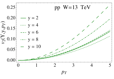
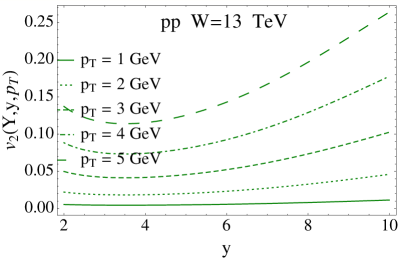
Fig. 5-a		Fig. 5-b
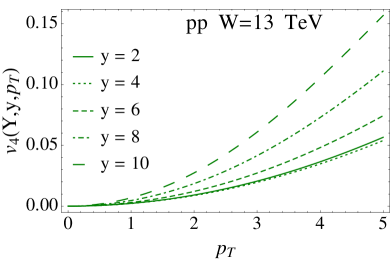
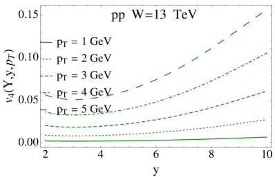
Fig. 5-c		Fig. 5-d

Figure 5: $v_{n}$ versus $p_{T}$ (Fig. 5-a and Fig. 5-c) and versus $y$ (Fig. 5-b and Fig. 5-d) at W=13 TeV assuming that the experiment has a symmetric pattern with $Y-y_{1}=y_{2}=\frac{1}{2}(Y-y_{12})$. In all these figures we use Eq. (6) for normalization and we take $\Delta_{\rm BFKL}=0.25$ and $Q^{2}_{s}(Y)\propto\exp\left(\lambda Y\right)$ with $\lambda=0.25$. These numbers correspond to the BFKL phenomenology.

Fig. 5 shows the $p_{T}$ and $y$ dependence of the $v_{2}$ and $v_{4}$ using Eq. (6) for normalization. In addition we take $\Delta_{\rm BFKL}$ = 0.25 and $Q^{2}_{s}(y)\,\propto\,\exp\left(\lambda\,y\right)$ with $\lambda=0.25$. These values correspond to the BFKL Pomeron phenomenology. We believe that this figure illustrates the scale of rapidity dependence and will be instructive for future experimental observations.

7 Conclusions

In this paper we generalize the interference diagram, that described the Bose-Einstein correlation for small rapidity difference $\bar{\alpha}_{S}y_{12}\,\ll\,1$, to include the emission of the gluons with rapidities ($y_{i}$) between $y_{1}$ and $y_{2}$ ($y_{1}\,,\,y_{i}\,<\,y_{2}$). We calculate the resulting diagram in CGC/saturation approach and make two observations which we consider as the main result of this paper. The first one is a substantial decrease of the odd Fourier harmonics $v_{2n+1}$ as a function of the rapidity difference $y_{12}$ ( see Fig. 4-c). The second result is, that even Fourier harmonic $v_{2n}$ has a rather strong dependence on $y_{12}$, showing a considerable increase in the region of large $y_{12}$ ( see Fig. 5). We believe that our calculations, that have been performed both for the simplest diagrams and for the CGC/saturation approach, will be instructive for further development of the approach especially in the part that is related to the integration of the momenta transferred by the BFKL Pomerons.

We demonstrated in this paper the general origin of the density variation mechanism, whose nature does not depend on the technique that has been used. This mechanism has to be taken into account, since it leads to the values of Fouriers harmonics that are large and of the order of $v_{n}$ that have been observed experimentally.

We hope that the paper will be useful in the clarification of the origin of the angular correlation, especially for hadron-hadron scattering at high energy. We firmly believe that the experimental observation of both phenomena: the sharp decrease of $v_{n}$ with odd $n$ and the substantial increase of $v_{n}$ with even $n$ as a function of $y_{12}$, will be a strong argument for CGC/saturation nature of the angular correlations.

8 Acknowledgements

We thank our colleagues at Tel Aviv university and UTFSM for encouraging discussions. Our special thanks go to Carlos Contreras, Alex Kovner and Misha Lublinsky for elucidating discussions on the subject of this paper.

This research was supported by the BSF grant 2012124, by Proyecto Basal FB 0821(Chile) , Fondecyt (Chile) grant 1140842, and by CONICYT grant PIA ACT1406.

References

- (1) A. Dumitru, F. Gelis, L. McLerran and R. Venugopalan, Nucl. Phys. A 810 (2008) 91 [arXiv:0804.3858 [hep-ph]].
- (2) E. V. Shuryak, Phys. Rev. C 76 (2007) 047901 [arXiv:0706.3531 [nucl-th]]; S. A. Voloshin, Phys. Lett. B 632 (2006) 490 [nucl-th/0312065]; S. Gavin, L. McLerran and G. Moschelli,= Phys. Rev. C 79 (2009) 051902 [arXiv:0806.4718 [nucl-th]].
- (3) K. Dusling and R. Venugopalan, Phys. Rev. D 87 (2013) no.9, 094034, [arXiv:1302.7018 [hep-ph]] and reference therein.
- (4) A. Kovner and M. Lublinsky, Phys. Rev. D 83, 034017 (2011), [arXiv:1012.3398 [hep-ph]].
- (5) Y. V. Kovchegov and D. E. Wertepny, Nucl. Phys. A 906 (2013) 50, [arXiv:1212.1195 [hep-ph]];
- (6) T. Altinoluk, N. Armesto, G. Beuf, A. Kovner and M. Lublinsky, Phys. Lett. B 752 (2016) 113, [arXiv:1509.03223 [hep-ph]]; T. Altinoluk, N. Armesto, G. Beuf, A. Kovner and M. Lublinsky, Phys. Lett. B 751 (2015) 448, [arXiv:1503.07126 [hep-ph]].
- (7) E. Gotsman, E. Levin, U. Maor and S. Tapia, Phys. Rev. D 93 (2016) no.7, 074029, [arXiv:1603.02143 [hep-ph]].
- (8) E. Gotsman, E. Levin and U. Maor, Phys. Rev. D 95, no. 3, 034005 (2017) [arXiv:1604.04461 [hep-ph]].
- (9) E. Gotsman and E. Levin, Phys. Rev. D 95 (2017) no.1, 014034 [arXiv:1611.01653 [hep-ph]].
- (10) A. Kovner, M. Lublinsky and V. Skokov, Phys. Rev. D 96 (2017) 016010 [ arXiv:1612.07790 [hep-ph]].
- (11) E. .Gotsman, E. Levin and I. Potashnikova, Eur. Phys. J. C 77 (2017) 632 [arXiv:1706.07617 [hep-ph]].
- (12) V. Khachatryan et al. [CMS Collaboration], Phys. Rev. Lett. 116 (2016) 172302[ arXiv:1510.03068 [nucl-ex]]; JHEP 1009 (2010) 091 [arXiv:1009.4122 [hep-ex]]. Phys. Rev. Lett. 116 (2016) 172302[ arXiv:1510.03068 [nucl-ex]].
- (13) J. Adams et al. [STAR Collaboration], Phys. Rev. Lett. 95 (2005) 152301 [arXiv: 0501016[nucl-ex]].
- (14) B. Alver et al. [PHOBOS Collaboration], Phys. Rev. Lett. 104 (2010) 062301 [arXiv:0903.2811 [nucl-ex]].
- (15) H. Agakishiev et al. [STAR Collaboration], “Measurements of Dihadron Correlations Relative to the Event Plane in Au+Au Collisions at GeV,” arXiv:1010.0690 [nucl-ex].
- (16) S. Chatrchyan et al. [CMS Collaboration], Phys. Lett. B 718 (2013) 795 [arXiv:1210.5482 [nucl-ex]]; V. Khachatryan et al. [CMS Collaboration], JHEP 1009 (2010) 091, [arXiv:1009.4122 [hep-ex]].
- (17) S. Chatrchyan et al. [CMS Collaboration], JHEP 1402 (2014) 088, [arXiv:1312.1845 [nucl-ex]]; Phys. Rev. C 89 (2014) no.4, 044906; [arXiv:1310.8651 [nucl-ex]]; Eur. Phys. J. C 72 (2012) 2012 [arXiv:1201.3158 [nucl-ex]]; JHEP 1402 (2014) 088, [arXiv:1312.1845 [nucl-ex]].
- (18) J. Adam et al. [ALICE Collaboration], Phys. Rev. Lett. 117 (2016) 182301, arXiv:1604.07663 [nucl-ex]; Phys. Rev. Lett. 116 (2016) no.13, 132302, [arXiv:1602.01119 [nucl-ex]]; L. Milano [ALICE Collaboration], Nucl. Phys. A 931 (2014) 1017, [arXiv:1407.5808 [hep-ex]]; Y. Zhou [ALICE Collaboration], J. Phys. Conf. Ser. 509 (2014) 012029, [arXiv:1309.3237 [nucl-ex]].
- (19) B. B. Abelev et al. [ALICE Collaboration], Phys. Rev. C 90 (2014) no.5, 054901, [arXiv:1406.2474 [nucl-ex]]; B. B. Abelev et al. [ALICE Collaboration], Phys. Lett. B 726 (2013) 164, [arXiv:1307.3237 [nucl-ex]]; B. Abelev et al. [ALICE Collaboration], Phys. Lett. B 719 (2013) 29, [arXiv:1212.2001 [nucl-ex]].
- (20) M. Aaboud et al. [ATLAS Collaboration], Phys. Rev. C 96 (2017) 024908 [ arXiv:1609.06213 [nucl-ex]]. G. Aad et al. [ATLAS Collaboration], Phys. Rev. Lett. 116 (2016) 172301 [arXiv:1509.04776 [hep-ex]].
- (21) G. Aad et al. [ATLAS Collaboration], Phys. Rev. C 90 (2014) no.4, 044906; [arXiv:1409.1792 [hep-ex]]; B. Wosiek [ATLAS Collaboration], Annals Phys. 352 (2015) 117; G. Aad et al. [ATLAS Collaboration], Phys. Lett. B 725 (2013) 60, [arXiv:1303.2084 [hep-ex]].
- (22) B. Wosiek [ATLAS Collaboration], Phys. Rev. C 86 (2012) 014907, [arXiv:1203.3087 [hep-ex]].
- (23) V. A. Abramovsky, V. N. Gribov and O. V. Kancheli, Yad. Fiz. 18, 595 (1973) [Sov. J. Nucl. Phys. 18, 308 (1974)].
- (24) A. H. Mueller, Phys. Rev. D2 (1970) 2963.
- (25) E. A. Kuraev, L. N. Lipatov, and F. S. Fadin, Sov. Phys. JETP 45, 199 (1977); Ya. Ya. Balitsky and L. N. Lipatov, Sov. J. Nucl. Phys. 28, 22 (1978).
- (26) L. N. Lipatov, Phys. Rep. 286 (1997) 131; Sov. Phys. JETP 63 (1986) 904 and references therein.
- (27) Yuri V Kovchegov and Eugene Levin, “ Quantum Choromodynamics at High Energies", Cambridge Monographs on Particle Physics, Nuclear Physics and Cosmology, Cambridge University Press, 2012 .
- (28) Y. V. Kovchegov, Phys. Rev. D 64, 114016 (2001) [Erratum-ibid. D 68, 039901 (2003)] [arXiv:hep-ph/0107256].
- (29) Y. V. Kovchegov and K. Tuchin, Phys. Rev. D 65, 074026 (2002) [arXiv:hep-ph/0111362].
- (30) J. Jalilian-Marian and Y. V. Kovchegov, Phys. Rev. D 70, 114017 (2004) [Erratum-ibid. D 71, 079901 (2005)] [arXiv:hep-ph/0405266].
- (31) M. A. Braun, Eur. Phys. J. C 48, 501 (2006) [arXiv:hep-ph/0603060]; Eur. Phys. J. C 55 (2008) 377, [arXiv:0801.0493 [hep-ph]].
- (32) C. Marquet, Nucl. Phys. B 705, 319 (2005) [arXiv:hep-ph/0409023].
- (33) A. Kovner and M. Lublinsky, JHEP 0611, 083 (2006) [arXiv:hep-ph/0609227].
- (34) E. Levin and A. Prygarin, Phys. Rev. C 78, 065202 (2008), [arXiv:0804.4747 [hep-ph]].
- (35) J. Jalilian-Marian and Y. V. Kovchegov, Phys. Rev. D 70, 114017 (2004) [Erratum-ibid. D 71, 079901 (2005), [arXiv:hep-ph/0405266].
- (36) K. G. Boreskov, A. B. Kaidalov and O. V. Kancheli, Eur. Phys. J. C 58 (2008) 445, [arXiv:0809.0625 [hep-ph]].
- (37) E. Levin and A. H. Rezaeian, Phys. Rev. D 84, 034031 (2011) [arXiv:1105.3275 [hep-ph]].
- (38) Y. Hagiwara, Y. Hatta, B. W. Xiao and F. Yuan, Phys. Lett. B 771 (2017) 374, [arXiv:1701.04254 [hep-ph]].
- (39) L. McLerran and V. Skokov, Nucl. Phys. A 947 (2016) 142, [arXiv:1510.08072 [hep-ph]].
- (40) A. Kovner and M. Lublinsky, Int. J. Mod. Phys. E 22, 1330001 (2013), [arXiv:1211.1928 [hep-ph]] and references therein.
- (41) H. Navelet and R. B. Peschanski, Nucl. Phys. B 507, 35 (1997) [hep-ph/9703238]; Phys. Rev. Lett. 82 (1999) 1370 [hep-ph/9809474]; Nucl. Phys. B 634 (2002) 291 [hep-ph/0201285].
- (42) I. Gradstein and I. Ryzhik, Table of Integrals, Series, and Products, Fifth Edition, Academic Press, London, 1994
- (43) L. V. Gribov, E. M. Levin and M. G. Ryskin, Phys. Rep. 100 (1983) 1.
- (44) A. H. Mueller and J. Qiu, Nucl. Phys. B268 (1986) 427.
-
(45)
L. McLerran and R. Venugopalan,
Phys. Rev. D49 (1994) 2233, 3352; D50 (1994) 2225;
D53 (1996) 458;
D59 (1999) 09400. - (46) A. H. Mueller and D. N. Triantafyllopoulos, Nucl. Phys. B 640, 331 (2002); [hep-ph/0205167].
- (47) E. Iancu, K. Itakura and L. McLerran, Nucl. Phys. A 708 (2002) 327, [hep-ph/0203137]; A. M. Stasto, K. J. Golec-Biernat and J. Kwiecinski, Phys. Rev. Lett. 86 (2001) 596, [hep-ph/0007192]; E. Levin and K. Tuchin, Nucl. Phys. B 573 (2000) 833, [hep-ph/9908317]. J. Bartels and E. Levin, Nucl. Phys. B 387 (1992) 617.
- (48) E. Levin and K. Tuchin, Nucl. Phys. B 573 (2000) 833, [hep-ph/9908317].
- (49) C. Contreras, E. Levin, R. Meneses and I. Potashnikova, Phys. Rev. D 94 (2016) no.11, 114028; [arXiv:1607.00832 [hep-ph]].
- (50) C. Contreras, E. Levin and I. Potashnikova, Nucl. Phys. A 948 (2016) 1, [arXiv:1508.02544 [hep-ph]].
- (51) E. Iancu, K. Itakura and S. Munier, Phys. Lett. B 590 (2004) 199 [arXiv: 0310338[hep-ph]].
- (52) J. Jalilian-Marian and Y. V. Kovchegov, Phys. Rev. D 70, 114017 (2004) [Erratum-ibid. D 71, 079901 (2005), [arXiv:hep-ph/0405266].
- (53) E. Gotsman and E. Levin, Bose-Einstein correlations in perturbative QCD: dependence on multiplicity, Phys. Rev. D ( in press)[ arXiv:1705.07406 [hep-ph]].