On connection coefficients, zeros and interception points of some perturbed of arbitrary order of the Chebyshev polynomials of second kind

Abstract

Orthogonal polynomials satisfy a recurrence relation of order two, where appear two coefficients. If we modify one of these coefficients at a certain order, we obtain a perturbed orthogonal sequence. In this work we consider in this way some perturbed of Chebyshev polynomials of second kind and we deal with the problem of finding the connection coefficients that allow to write the perturbed sequence in terms of the original one and in terms of the canonical basis. From the connection relations obtained and from two other relations, we deduce some results about zeros and interception points of these perturbed polynomials. All the work is valid for arbitrary order of perturbation.

Key words: Chebyshev polynomials; perturbed orthogonal polynomials; connection coefficients; zeros.

2010 Mathematics Subject Classification: 33C45, 33D45, 42C05.

1 Introduction

Perturbed orthogonal polynomials are obtained by modifying, in a certain way, a finite number of elements of the two sequences of coefficients presented in the linear recurrence relation of order two satisfied by these polynomials. In this work, we focus our attention on elementary modifications of only one of these two coefficients at a unique specified order $r$, the so-called, in literature, generalized co-recursive or co-dilated polynomials. During the last decades, this subject have interested several authors. We would like to cite, with respect to the co-recursive case ($r=0$), the references [9, 10, 25, 29, 52, 55]; concerning the co-dilated situation, we consider [17, 41]; for the co-modified sequences refer to [14, 15, 51]; for the generalized co-polynomials see [6, 18, 32]. Also, we call the attention to the general articles [47, 59]. We notice that perturbed orthogonal polynomials have some applications, which motivate further their study [17, 26, 27, 29, 32, 55]. This type of perturbation is a transformation that can promote a significative change of properties of the original sequence, but the second degree character is preserved by it [35, 38]. The PSDF algorithm (see [12]) allows to explicit some semi-classical properties of perturbed second degree forms leading, in special, to the second order linear differential equation. It is well known that the four Chebyshev sequences [21, 22, 46] are the most important cases of second degree forms [39]. In particular, for the purposes of perturbation, the family of second kind is the most simple among them, because it is self-associated [40], therefore it is often taken as study case in the mentioned literature. There are some specific works about perturbed Chebyshev families, namely [41] about the co-dilated case of the second kind form, and [39, 53] concerning all the four forms. Also, in [13], we present some semi-classical properties obtained with PSDF [12] for the second kind sequence corresponding to the complete perturbation of order 1 and the perturbation of 2 by dilatation, generalizing most known results. In [12], we give similar properties for the co-recursive and co-dilated sequences of order 3.

In the present work, we focus our attention on connection coefficients and some consequences related to zeros and interception points valid for any order $r$ of perturbation of the second kind Chebyshev sequence.

About connection coefficients for orthogonal polynomials the reader can find an extensive bibliography in [57]. In fact, the literature on this subject is vast and a wide variety of methods have been developed using several techniques. Here, we refer mainly to the following references [1, 2, 3, 8, 11, 24, 30, 31, 49, 50, 56]. Zeros of orthogonal polynomials is another widely discussed subject due to its applications in several problems of applied sciences [54] and their crucial role in quadrature formulas [22]. In particular, several authors have dedicated attention to the relationship between the zeros of perturbed polynomials and the zeros of the original sequences finding results about interlacing and monotonicity behaviors and distribution functions for co-recursive and co-dilated cases, see [9, 25, 28, 32, 52, 54, 55], and more recently [6, 7, 17].

Let us summarize the contents of this article. In Section 2, we present the theoretical background concerning orthogonal polynomials [10, 35], perturbation [10, 32, 35], connection coefficients [42, 43] and properties of the four families of Chebyshev polynomials [46]. It is natural to consider the first, third and four kinds Chebyshev families as perturbed of the sequence of second kind [13]. From this point on, we shall deal only with the second kind Chebyshev family and its elementary perturbations of order $r$ by translation and by dilatation [12]. The contribution of this article is focused on finding explicit results about connection coefficients and some of their consequences valid for any order of perturbation. We think that this point is important, because thus one can choose the parameter of perturbation and its order in such a way a prescribed behavior occurs, for example, the positiveness of connection coefficients or the location of certain zeros or interception points. Section 3 is dedicated to the connection coefficients that allow to write the perturbed family in terms of the original one (Section 3.1) and in terms of the canonical basis (Section 3.2). We started this study from some tables of the first connection coefficients, for fixed values of the order $r$ of perturbation, recursively computed by the symbolic software CCOP - Connection Coefficients for Orthogonal Polynomials [43, 44, 45]. We realize that the connection coefficients are constant by diagonal and have very simple expressions, therefore it was easy to infer closed formulas valid for any $r$. Demonstrations of these formulas will be done by induction. From the connection relations deduced in Section 3.1 and from the connection coefficients of the second kind Chebyshev family in terms of the canonical basis, we deduce in Section 3.2, the connection coefficients of perturbed polynomials in terms of the canonical basis. Section 4 concerns some results about zeros and interception points of perturbed polynomials. We begin by presenting the Hadamard–Gershgörin location of zeros. We determine the values of the parameters of perturbation for which there are zeros outside the interval $[-1,1]$. After that, results are deduced from the connection relations previously obtained and from two other relations. We point out the fact that the behavior of perturbed polynomials at the origin are related to the parity of $r$. Depending on the values of the parameters of perturbation, the smallest and the greatest zeros of perturbed polynomials have a special location with respect to the extremal zeros of Chebyshev polynomials of the same degree. Perturbed polynomials with fixed degree and different values of parameters intercept each other at the zeros of two other Chebyshev polynomials with prescribed degrees: these points are stable, they do not depend on perturbation. Interceptions points can be simple or double depending on the degrees of polynomials and their relationship with $r$. We distinguish the interceptions points that are common zeros. In the last section, we present some graphical representations in order to illustrate results given herein about zeros and interception points. In fact, these graphs were the source of inspiration to the development of this study. The reasonings and arguments employed in the proofs are similar for the translation and the dilatation cases, but the dilatation one is more simple, because perturbed sequences are symmetric. We remark that zeros of perturbed Chebyshev polynomials satisfy some interlacing and monotonicity properties, not studied here, that can be the subject for a forthcoming article.

2 Theoretical background

2.1 Connection coefficients for perturbed orthogonal polynomials

Let $\mathcal{P}$ be the vector space of polynomials with coefficients in $\mathbb{C}$ and let $\mathcal{P}^{\prime}$ be its topological dual space. We denote by $\langle u,p\rangle$ the effect of $u\in\mathcal{P}^{\prime}$ on $p\in\mathcal{P}$. In particular, $\langle u,x^{n}\rangle:=\nolinebreak\left(u\right)_{n},n\geq 0$, represent the moments of $u$. A form $u$ is normalized if its first moment is unit, e.g., $(u)_{0}=1$. Let $\{P_{n}\}_{n\geq 0}$ be a monic polynomial sequence (MPS) with $\deg P_{n}=n,\ n\geq 0$, e.g., $P_{n}(x)=x^{n}+\ldots$. Then there exists a unique sequence $\{u_{n}\}_{n\geq 0}$, $u_{n}\in\mathcal{P}^{\prime}$, called the dual sequence of $\{P_{n}\}_{n\geq 0}$, such that $<u_{n},P_{m}>=\delta_{n,m}$, $n,m\geq 0$. The form $u_{0}$ is called the canonical form of $\{P_{n}\}_{n\geq 0}$, it is normalized, e.g., $(u_{0})_{0}=1$.

A form $u$ is said regular [36, 37] if and only if there exists a polynomial sequence $\{P_{n}\}_{n\geq 0}$, such that:

$$\left\langle u,P_{n}P_{m}\right\rangle = 0\ ,\ n\neq m\ ,\ n,m\geq 0\ ,$$ (1)

$$\left\langle u,P^{2}_{n}\right\rangle=k_{n} \neq 0\ ,\ n\geq 0\ .$$ (2)

Consequently $\deg P_{n}=n$, $n\geq 0$, and any $P_{n}$ can be taken monic, then $\{P_{n}\}_{n\geq 0}$ is called a monic orthogonal polynomial sequence (MOPS) with respect to $u$. Necessarily $u=(u)_{0}u_{0}$, $(u)_{0}\not=0$. If we take $u$ normalized, then $u=u_{0}$. In this work, we will always consider MOPS and normalized forms. The identities (1) are called the orthogonality conditions and (2) are the regularity conditions.

The sequence $\{P_{n}\}_{n\geq 0}$ is regularly orthogonal with respect to $u$ if and only if [36, 37] there are two sequences of coefficients $\{\beta_{n}\}_{n\geq 0}$ and $\{\gamma_{n+1}\}_{n\geq 0}$, with $\gamma_{n+1}\neq 0,\;n\geq 0$, such that, $\{P_{n}\}_{n\geq 0}$ satisfies the following initial conditions and linear recurrence relation of order 2

$$P_{0}(x)=1,\quad P_{1}(x)=x-\beta_{0},$$ (3)

$$P_{n+2}(x)=(x-\beta_{n+1})P_{n+1}(x)-\gamma_{n+1}P_{n}(x),\quad n\geq 2.$$ (4)

Furthermore, the recurrence coefficients $\{\beta_{n}\}_{n\geq 0}$ and $\{\gamma_{n+1}\}_{n\geq 0}$ satisfy:

$$\beta_{n} = \frac{\left\langle u,xP_{n}^{2}(x)\right\rangle}{k_{n}},\quad n\geq 0,$$

$$\gamma_{n+1} = \frac{k_{n+1}}{k_{n}},\quad n\geq 0.$$ (5)

We remark that, from (3) and (5), the regularity conditions (2) are equivalent to the conditions $\gamma_{n+1}\neq 0,\ n\geq 0$. As usual, we suppose that, $\beta_{n}=0$, $\gamma_{n+1}=0$ and $P_{n}(x)=0$, for all$n<0$.

The MOPS $\{P_{n}\}_{n\geq 0}$ is real if and only if $\beta_{n}\in\mathbb{R}$ and $\gamma_{n+1}\in\mathbb{R}-\{0\}$. These conditions are equivalent to $(u)_{n}\in\mathbb{R},\ n\geq 0$ and $u$ is real. If, in addition, we suppose that $\gamma_{n+1}>0$, $n\geq 0$, then $u$ is positive definite, because this condition is equivalent to $<u,p>>0$, $\forall p\in{\cal P}$: $p\not\equiv 0$, $p(x)\geq 0$, $x\in\mathbb{R}$ [10, 35].

A form $u$ is symmetric if and only if $(u)_{2n+1}=0,\ n\geq 0.$ A polynomial sequence, $\{P_{n}\}_{n\geq 0}$, is symmetric if and only if $P_{n}(-x)=(-1)^{n}P_{n}(x),\ n\geq 0.$ If $\{P_{n}\}_{n\geq 0}$ is a MOPS with respect to $u$, then these conditions are equivalent to $\beta_{n}=0$, $n\geq 0$ [10, 35].

The $r$th-associated sequence of a MOPS $\{P_{n}\}_{n\geq 0}$ satisfying (3)-(4) is a MOPS $\{P^{(r)}_{n}\}_{n\geq 0}$ whose recurrence coefficients are given by [10, 35]

$$\beta_{n}^{(r)}=\beta_{n+r}\quad,\quad\gamma_{n+1}^{(r)}=\gamma_{n+1+r}\quad,\quad n\;,\;r\geq 0\;.$$ (6)

Let us consider two perturbed sequences of a MOPS $\{P_{n}\}_{n\geq 0}$ satisfying (3)-(4), obtained by modifying only one of its recurrence coefficients at order $r$. We shall modify $\beta_{r}$ by translation and $\gamma_{r}$ by dilatation by means of two parameters $\mu_{r}$ and $\lambda_{r}$. Thus, the $r$th-perturbed sequence by translation, for $r\geq 0$, noted by $\{P^{t}_{n}(\mu_{r};r)(x)\}_{n\geq 0}$, is a MOPS with the following recurrence coefficients

$$\beta^{t}_{r}=\beta_{r}+\mu_{r}\ ,\ \beta^{t}_{n}=\beta_{n}\ ,\ n\neq r\ ,\ n\geq 0\quad;\quad\gamma^{t}_{n+1}=\gamma_{n+1}\ ,\ n\geq 0\ .$$ (7)

When $r=0$, we recover the so-called co–recursive sequence [9, 10], for which only the initial polynomial $P_{1}(x)$ is perturbed becoming $P^{t}_{1}(\mu_{0};0)(x)=x-\beta_{0}-\mu_{0}$. The $r$th-perturbed sequence by dilatation, for $r\geq 1$, noted by $\{P^{d}_{n}(\lambda_{r};r)(x)\}_{n\geq 0}$, is a MOPS with the following recurrence coefficients

$$\beta^{d}_{n}=\beta_{n}\ ,\ n\geq 0\quad;\quad\gamma^{d}_{r}=\lambda_{r}\gamma_{r}\ ,\ \lambda_{r}\neq 0,1\ ,\ \gamma^{d}_{n+1}=\gamma_{n+1}\ ,\ n\neq r-1,\ n\geq 0\ .$$ (8)

We note by $\tilde{u}:=\displaystyle u^{t}\left(\mu_{r};r\right)$ and $\tilde{u}:=\displaystyle u^{d}\left(\lambda_{r};r\right)$, the forms with respect to which these families are orthogonal. In literature, these sequences are often designated as $r$th-generalized co-recursive and $r$th-generalized co-dilated polynomials and both situations as $r$th-generalized co-polynomials [32]. Also, they are particular cases of a general perturbation of order $r$ defined in [35]. Perturbation by translation destroys the symmetry, but does not change the positive definiteness character of the original sequence. Perturbation by dilatation does not change the symmetry; moreover if $\lambda_{r}>0$, it preserves also the positive definiteness character.

The canonical sequence $\{X_{n}\}_{n\geq 0}$, $X_{n}(x)=x^{n}$, is orthogonal with respect to the Dirac measure $\delta_{0}$, $\left\langle\delta_{0},f\right\rangle=f(0),\ {\rm defined\ by\ the\ moments}\left(\delta_{0}\right)_{n}={\delta}_{0,n},\ n\geq 0$. This sequence is not regularly orthogonal, since it satisfies (3)-(4) with recurrence coefficients

$$\beta_{n}=0\ ,\ \gamma_{n+1}=0\ ,\ n\geq 0\ .$$ (9)

Given any two MPS $\{P_{n}\}_{n\geq 0}$ and $\{{\tilde{P}}_{n}\}_{n\geq 0}$, not necessarily orthogonal, the coefficients that satisfy the connection relation (CR)

$${\tilde{P}}_{n}(x)=\sum_{m=0}^{n}\lambda_{n,m}^{{\tilde{P}}P}{P}_{m}(x),\ n\geq 0,$$ (10)

are called the connection coefficients (CC) $\lambda_{n,m}:=\lambda_{n,m}^{{\tilde{P}}P}:=\lambda_{n,m}({\tilde{P}}\leftarrow P)$. It is obvious that these coefficients exist and are unique, because the polynomial sequences are linearly independent. In the case $P_{m}(x)=X_{m}(x)=x^{m}$, $m\geq 0$, we have

$${\tilde{P}}_{n}(x)=\sum_{m=0}^{n}\lambda^{{\tilde{P}}X}_{n,m}x^{m},$$ (11)

with $\lambda^{{\tilde{P}}X}_{n,m}:=\lambda_{n,m}({\tilde{P}}\leftarrow X)$. We shall consider also the Viète’s formulas [58] that establish a relationship between $\lambda^{{\tilde{P}}X}_{n,m}$ and the zeros $\{\xi_{m}^{(n)}\}_{m=1(1)n}$ of ${\tilde{P}}_{n}$, in particular

$$\lambda^{{\tilde{P}}X}_{n,n-1}=-\sum_{m=1}^{n}\xi_{m}^{(n)}\quad,\quad\lambda^{{\tilde{P}}X}_{n,0}=(-1)^{n}\prod_{m=1}^{n}\xi_{m}^{(n)}\ ,\ n\geq 1\ .$$ (12)

Let us suppose that the MPS $\{P_{n}\}_{n\geq 0}$ is orthogonal with respect to $u$, then multiplying both members of (10) by $P_{k}(x)$, applying $u$ and taking into account (1) and (2), we obtain [42, p.295]

$$\lambda_{n,m}^{{\tilde{P}}P} = \frac{\left\langle u,{\tilde{P}}_{n}P_{m}\right\rangle}{k_{n}}\ ,\ 0\leq m\leq n\ ,\ n\geq 0\ .$$ (13)

In addition, let us suppose that the MPS $\{{\tilde{P}}_{n}\}_{n\geq 0}$ is orthogonal with respect to $\tilde{u}$, and that $\{P_{n}\}_{n\geq 0}$ and $\{{\tilde{P}}_{n}\}_{n\geq 0}$ are given by their recurrence coefficients $\{\beta_{n}\}_{n\geq 0}$, $\{\gamma_{n+1}\}_{n\geq 0}$ and $\{{\tilde{\beta}}_{n}\}_{n\geq 0}$, $\{{\tilde{\gamma}}_{n+1}\}_{n\geq 0}$, respectively. In (13), using (4) and (5) for both sequences, it is possible to demonstrate that the CC fulfill the following boundary and initial conditions and general recurrence relation [42, pp.295-296] (see, also, [43])

$$\lambda_{n,m}^{{\tilde{P}}P}=0\ ,\ n<0\text{\ or\ }m<0\text{\ or\ }m>n\ ;\ \lambda_{n,n}^{{\tilde{P}}P}=1\ ,\ n\geq 0\ ;\ \lambda^{{\tilde{P}}P}_{1,0}=\beta_{0}-{\tilde{\beta}}_{0}\ ,$$ (14)

$$\lambda^{{\tilde{P}}P}_{n,m}=\left({\beta}_{m}-{\tilde{\beta}}_{n-1}\right)\lambda^{{\tilde{P}}P}_{n-1,m}-{\tilde{\gamma}}_{n-1}\lambda^{{\tilde{P}}P}_{n-2,m}+{\gamma}_{m+1}\lambda^{{\tilde{P}}P}_{n-1,m+1}+\lambda^{{\tilde{P}}P}_{n-1,m-1}\ ,$$ (15)

$$\hskip 42.67912pt\ 0\leq m\leq n-1\ ,\ n\geq 2\ .$$

If $\{P_{n}\}_{n\geq 0}$ and $\{\tilde{P}_{n}\}_{n\geq 0}$ are symmetric, then from (13) and the symmetry of $u$, we have

$$\lambda_{2n-1,2m}^{{\tilde{P}}P}=0\ ,\ \lambda_{2n,2m+1}^{{\tilde{P}}P}=0\ ,\ 0\leq m\leq n-1\ ,\ n\geq 1\ .$$

Moreover, as $\beta_{n}=0=\tilde{\beta}_{n}$, $n\geq 0$, the relation (15) is equivalent to

$$\lambda_{2n,2m}^{{\tilde{P}}P} = {\gamma}_{2m+1}\lambda_{2n-1,2m+1}^{{\tilde{P}}P}+\lambda_{2n-1,2m-1}^{{\tilde{P}}P}-{\tilde{\gamma}}_{2n-1}\lambda_{2n-2,2m}^{{\tilde{P}}P}\ ,$$

$$\lambda_{2n+1,2m+1}^{{\tilde{P}}P} = {\gamma}_{2m+2}\lambda_{2n,2m+2}^{{\tilde{P}}P}+\lambda_{2n,2m}^{{\tilde{P}}P}-{\tilde{\gamma}}_{2n}\lambda_{2n-1,2m+1}^{{\tilde{P}}P}\ ,$$

for $0\leq m\leq n-1\ ,\ n\geq 1$. Furthermore, in the case $P_{n}\equiv X_{n}$, due to (9), these relations become

$$\lambda^{{\tilde{P}}X}_{2n,2m} = \lambda^{{\tilde{P}}X}_{2n-1,2m-1}-{\tilde{\gamma}}_{2n-1}\lambda^{{\tilde{P}}X}_{2n-2,2m}\ ,$$

$$\lambda^{{\tilde{P}}X}_{2n+1,2m+1} = \lambda^{{\tilde{P}}X}_{2n,2m}-{\tilde{\gamma}}_{2n}\lambda^{{\tilde{P}}X}_{2n-1,2m+1}\ .$$

2.2 The four families of Chebyshev polynomials

There are four sequences of Chebyshev polynomials, they are called Chebyshev polynomials of first ($T_{n}$), second ($P_{n}$), third ($V_{n}$) and fourth ($W_{n}$) kinds. W. Gaustchi [21] named these last two sequences in this way, before they had been designated as airfoil polynomials (see, e.g., [19]). Their trigonometric definitions are

$$T_{n}(x)=\frac{1}{2^{n-1}}\cos nt\quad \quad P_{n}(x)=\frac{1}{2^{n}}\frac{\sin(n+1)t}{\sin t}\ ,$$ ,

$$V_{n}(x)=\frac{1}{2^{n}}\frac{\cos(n+\frac{1}{2})t}{\cos\frac{1}{2}t}\quad \quad W_{n}(x)=\frac{1}{2^{n}}\frac{\sin(n+\frac{1}{2})t}{\sin\frac{1}{2}t}\;,$$ ,

where $x=\cos t$, $t\in[0,\pi]$, $n\geq 0$. Notice that, as in this work we always consider monic polynomials, thus some normalization constants must appear in the preceding definitions. From them, it is trivial to obtain explicit formulas for the zeros [46, pp.20-21]

$$T_{n}: \rho^{(n)}_{k}=\cos\left(\frac{(k-\frac{1}{2})\pi}{n}\right),\ k=1(1)n\ ;\ P_{n}: \xi^{(n)}_{k}=\cos\left(\frac{k\pi}{n+1}\right),\ k=1(1)n,$$ (16)

$$V_{n}: \rho^{(n)}_{k}=\cos\left(\frac{(k-\frac{1}{2})\pi}{n+\frac{1}{2}}\right),\ k=1(1)n\ ;\ W_{n}: \rho^{(n)}_{k}=\cos\left(\frac{k\pi}{n+\frac{1}{2}}\right),\ k=1(1)n.$$ (17)

Using some trigonometric identities, it can be shown that these families satisfy (3)-(4) with the following recurrence coefficients [46]

$$T_{n}: \beta_{n}=0\;,\,n\geq 0\; ,\quad\gamma_{1}=\frac{1}{2}\;,\;\gamma_{n+1}={\frac{1}{4}}\;,\;n\geq 1\;,$$

$$P_{n}: \beta_{n}=0\;,\,n\geq 0\; ,\quad\gamma_{n+1}={\frac{1}{4}}\;,\;n\geq 1\;,$$ (18)

$$V_{n}: \beta_{0}=\frac{1}{2}\;,\;\beta_{n}=0\;,n\geq 1\; ,\quad\gamma_{n+1}={\frac{1}{4}}\;,\;n\geq 0\;,$$

$$W_{n}: \beta_{0}=-\frac{1}{2}\;,\;\beta_{n}=0\;,n\geq 1\; ,\quad\gamma_{n+1}={\frac{1}{4}}\;,\;n\geq 0\;.$$

Therefore, $\{T_{n}\}_{n\geq 0}$ and $\{P_{n}\}_{n\geq 0}$ are symmetric, $\{V_{n}\}_{n\geq 0}$ and $\{W_{n}\}_{n\geq 0}$ are not; they are all positive definite. As $\{P_{n}\}_{n\geq 0}$ has the most simple recurrence coefficients, then it is natural to consider $\{T_{n}\}_{n\geq 0}$, $\{V_{n}\}_{n\geq 0}$ and $\{W_{n}\}_{n\geq 0}$ as perturbed of $\{P_{n}\}_{n\geq 0}$ as follows [13]

$$T_{n}(x)=P^{d}_{n}\left(2;1\right)(x)\ ,\ V_{n}(x)=P^{t}_{n}\left(\frac{1}{2};0\right)(x)\ ,\ W_{n}(x)=P^{t}_{n}\left(-\frac{1}{2};0\right)(x)\ .$$ (19)

With respect to the association, we have that $T^{(1)}_{n}\equiv V^{(1)}_{n}\equiv W^{(1)}_{n}\equiv P_{n};$ moreover $P^{(r)}_{n}\equiv P_{n}$, $\forall r\geq 0$, e.g., $P_{n}$ is a self-associated sequence [40].

The following CR that allow to express $\{T_{n}\}_{n\geq 0}$, $\{V_{n}\}_{n\geq 0}$ and $\{W_{n}\}_{n\geq 0}$ in terms of $\{P_{n}\}_{n\geq 0}$ are well known [46, pp.4,8]

$$T_{n+2}(x)=P_{n+2}(x)-\frac{1}{4}P_{n}(x)\ ,\ n\geq 0\ ,$$ (20)

$$V_{n+1}(x)=P_{n+1}(x)-\frac{1}{2}P_{n}(x)\ ,\ n\geq 0\ ,$$ (21)

$$W_{n+1}(x)=P_{n+1}(x)+\frac{1}{2}P_{n}(x)\ ,\ n\geq 0\ .$$ (22)

One goal of this article is to generalize these CR putting in the first member of them any perturbed polynomial $P^{t}_{n}(\mu_{r};r)(x)$ and $P^{d}_{n}(\lambda_{r};r)(x)$ of the sequence of second kind.

The CC $C_{n,m}=\lambda_{n,m}^{{P}X}$ and the CR of $\{P_{n}\}_{n\geq 0}$ in the canonical basis are [48, p.223]

$$P_{2n}(x)=\sum_{\nu=0}^{n}C_{2n,2\nu}x^{2\nu}\ ,$$ (23)

$$C_{2n,2\nu}=\frac{(-1)^{n-\nu}}{2^{2(n-\nu)}}\binom{n+\nu}{n-\nu},\ \nu=0(1)n,\ C_{2n,2\nu+1}=0,\ \nu=0(1)n-1\ ;$$ (24)

$$P_{2n+1}(x)=\sum_{\nu=0}^{n}C_{2n+1,2\nu+1}x^{2\nu+1}\ ,$$ (25)

$$\ C_{2n+1,2\nu+1}=\frac{(-1)^{n-\nu}}{2^{2(n-\nu)}}\binom{n+\nu+1}{n-\nu},\ \nu=0(1)n,\ C_{2n+1,2\nu}=0,\ \nu=0(1)n\ .$$ (26)

Another goal of this article is to generalize these well known CC and CR putting in the first member of them any perturbed polynomial $P^{t}_{n}(\mu_{r};r)(x)$ and $P^{d}_{n}(\lambda_{r};r)(x)$ of the sequence of second kind. From the above identities, we obtain, in particular, that

$$C_{n,n-1}=0\ ,\ C_{2n,0}=\frac{(-1)^{n}}{2^{2n}}\ ,\ C_{2n+1,0}=0\ ,\ n\geq 0\ ,$$ (27)

which implies, by (12), that

$$\sum_{k=1}^{n}{\xi}_{k}^{(n)}=0\ ,$$ (28)

$$\prod_{k=1}^{2n}{\xi}_{k}^{(2n)}=\frac{(-1)^{n}}{2^{2n}}\Longrightarrow P_{2n}(0)\neq 0\ ,\prod_{k=1}^{2n+1}{\xi}_{k}^{(2n+1)}=0\Longrightarrow P_{2n+1}(0)=0\ .$$ (29)

We remark that $C_{2n,2\nu+1}=0$, $\nu=0(1)n-1$, $C_{2n+1,2\nu}=0$ and $P_{2n+1}(0)=0$, $n\geq 0$ are assured by symmetry.

The four kinds of Chebyshev polynomials [21, 46] belong to the Jacobi class of classical polynomials $\{P_{n}^{(\alpha,\beta)}(x)\}_{n\geq 0}$ [36, 37] orthogonal with respect to the form $\mathcal{J}(\alpha,\beta)$. A Jacobi form is regular if and only if $\alpha\neq-n$, $\beta\neq-n$, $\alpha+\beta\neq-(n+1)$, $n\geq 1$; it is symmetric for $\alpha=\beta$; it is positive definite if and only if $\alpha+1>0$ and $\beta+1>0$ and has the following integral representation for $Re(1+\alpha)>0$ and $Re(1+\beta)>0$ [10, 36, 37]

$$<\mathcal{J}(\alpha,\beta),f>=\frac{1}{2^{\alpha+\beta+1}}\frac{\Gamma(\alpha+\beta+2)}{\Gamma(\alpha+1)\Gamma(\beta+1)}\int_{-1}^{1}(1+x)^{\alpha}(1-x)^{\beta}f(x)dx\;.$$

Let us note the Chebyshev normalized forms by ${\cal T}_{1}$ $(\alpha=\beta=-\frac{1}{2})$, ${\cal U}$ $(\alpha=\beta=\frac{1}{2})$, ${\cal T}_{3}$ $(\alpha=\frac{1}{2},\ \beta=-\frac{1}{2})$ and ${\cal T}_{4}$ $(\alpha=-\frac{1}{2},\ \beta=\frac{1}{2})$ ; their integral representations are given by [46]

$$<{\cal T}_{1},f>=\frac{1}{\pi}\int_{-1}^{+1}\frac{f(x)}{\sqrt{1-x^{2}}}dx <{\cal U},f>=\frac{2}{\pi}\int_{-1}^{1}f(x)\sqrt{1-x^{2}}dx\ ,$$ , (30)

$$<{\cal T}_{3},f>=\frac{1}{\pi}\int_{-1}^{1}f(x)\sqrt{\frac{1+x}{1-x}}dx <{\cal T}_{4},f>=\frac{1}{\pi}\int_{-1}^{1}f(x)\sqrt{\frac{1-x}{1+x}}dx\ .$$ , (31)

Chebyshev forms are of second degree [4]. Perturbed Chebyshev polynomials are also of second degree and consequently they are semi-classical [38, 39]; the PSDF - Perturbed Second Degree Forms symbolic algorithm [12] allowed to explicit some of their main properties, namely the second order linear differential equation [13, 12]. Integral representations of perturbed Chebyshev forms are given in the co-recursive case in [9] and in the co-dilated situation of order 1 in [41]. To the best of my knowledge, these integral representations remain an open problem for orders of perturbation greater than or equal to two.

From now on, $\{P_{n}\}_{n\geq 0}$ will note the sequence of monic Chebyshev polynomials of second kind.

3 Connection coefficients and connection relations in terms of the Chebyshev polynomials of second kind

In this section, we shall give the CC and the CR that allow to express $\{P^{t}_{n}(\mu_{r};r)(x)\}_{n\geq 0}$ and $\{P^{d}_{n}(\mu_{r};r)(x)\}_{n\geq 0}$ in terms of $\{P_{n}\}_{n\geq 0}$, for any order $r$ of perturbation. That is, we shall deal with

$$\lambda^{t}_{n,m}:=\lambda^{P^{t}P}_{n,m}=\lambda_{n,m}(P^{t}(\mu_{r};r)\leftarrow P)\ {\rm and}\ \lambda^{d}_{n,m}:=\lambda^{P^{d}P}_{n,m}=\lambda_{n,m}(P^{d}(\lambda_{r};r)\leftarrow P)\ .$$

We begin by two lemmas, where we rewrite the general recurrence relation (14)-(15) in the two particular cases considered, replacing $\{\beta_{n}\}_{n\geq 0}$, $\{\gamma_{n+1}\}_{n\geq 0}$ and $\{{\tilde{\beta}}_{n}\}_{n\geq 0}$, $\{\tilde{\gamma}_{n+1}\}_{n\geq 0}$ by their particular values obtained from (7), (8) and (18) and given by

$$\beta_{r}^{t}=\mu_{r}\ ,\ \beta_{n}^{t}=0,\ n\neq r\ ;\ \gamma_{n+1}^{t}=\frac{1}{4}\ ,\ n\geq 0\ ,\ r\geq 0\ ,\ {\rm or}$$ (32)

$$\beta_{n}^{d}=0\ ;\ \gamma_{r}^{d}=\lambda_{r}\frac{1}{4}\ ,\ \gamma_{n+1}^{d}=\frac{1}{4},\ n\neq r-1\ ,\ n\geq 0\ ,\ r>0\ .$$ (33)

Lemma 3.1

For the co-recursive case $(r=0)$,

$$\lambda^{t}_{n,n}=1,\ n\geq 0\ ;\ \lambda^{t}_{1,0}=-\mu_{0}\ ;$$ (34)

$$\lambda^{t}_{n,m}=\frac{1}{4}\left(-\lambda^{t}_{n-2,m}+\lambda^{t}_{n-1,m+1}\right)+\lambda^{t}_{n-1,m-1}\ ,\ 0\leq m<n\ ,\ n\geq 2\ .$$ (35)

For the $r$th-perturbed by translation case $(r\geq 1)$,

$$\lambda^{t}_{n,n}=1,\ n\geq 0\ ;\ \lambda^{t}_{1,0}=0\ ;$$ (36)

$$\lambda^{t}_{r+1,m}=-\mu_{r}\lambda^{t}_{r,m}+\frac{1}{4}\left(-\lambda^{t}_{r-1,m}+\lambda^{t}_{r,m+1}\right)+\lambda^{t}_{r,m-1}\ ,\ 0\leq m<r+1\ ;$$ (37)

$$\lambda^{t}_{n,m}=\frac{1}{4}\left(-\lambda^{t}_{n-2,m}+\lambda^{t}_{n-1,m+1}\right)+\lambda^{t}_{n-1,m-1},\ 0\leq m<n,n\neq r+1,n\geq 2.$$ (38)

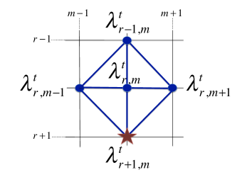
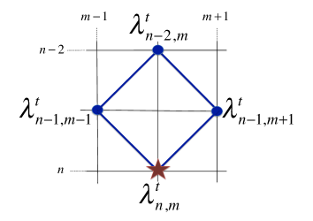
Figure 1: Representation of recurrence relations (37) and (38) for the $r$th-perturbed by translation case for $r\geq 1$.

Lemma 3.2

For the $r$th-perturbed by dilatation case $(r\geq 1)$,

$$\lambda^{d}_{n,n}=1,\ n\geq 0\ ;\ \lambda^{d}_{1,0}=0\ ;$$ (39)

$$\lambda^{d}_{r+1,m}=\frac{1}{4}\left(-\lambda_{r}\lambda^{d}_{r-1,m}+\lambda^{d}_{r,m+1}\right)+\lambda^{d}_{r,m-1}\ ,\ 0\leq m<r+1\ ;$$ (40)

$$\lambda^{d}_{n,m}=\frac{1}{4}\left(-\lambda^{d}_{n-2,m}+\lambda^{d}_{n-1,m+1}\right)+\lambda^{d}_{n-1,m-1},\ 0\leq m<n,n\neq r+1,n\geq 2.$$ (41)

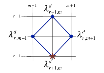
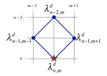
Figure 2: Representation of recurrence relations (40) and (41) for the $r$th-perturbed by dilatation case for $r\geq 1$.

The software CCOP - Connection Coefficients for Orthogonal Polynomials [44, 45] (see, also, [42]) written in the Mathematica^® language, includes an implementation of the recurrence relations (14)-(15) that allows the symbolic recursive computation of the first CC from the recurrence coefficients of the two polynomial sequences involved. In the cases under study, CCOP produced the results given in Tables 1 and 2 for the perturbation of order $r=3$. From these results and others, we discover that CC are constant by downward diagonal with very simple expressions and it was easy to infer the closed formulas corresponding to an arbitrary order $r$ of perturbation and any nonnegative integers $n$ and $m$. It was by this procedure that we formulate Theorems 3.3 and 3.4, and Propositions 3.5 and 3.6 presented next. Tables 3 and 4 generalize Table 1 for any odd or even orders ($r\geq 0$) in the translation case; Tables 5 and 6 generalize Table 2 for any odd or even orders ($r\geq 1$) in the dilatation case. In fact, there are slight differences depending on the parity of $r$.

Table 1: CC for the 3rd-perturbed by translation case with parameter $\mu_{3}$.

$\begin{array}[]{| l | l l l l | l ll l |lllll}\hline\cr m&0&1&2&3&4&5&6&7&8&9&10&11&\ldots\\ n&&&&&&&&&&&&&\\ \hline\cr 0&1&\text{}&\text{}&\text{}&\text{}&\text{}&\text{}&\text{}&\text{}&\text{}&\text{}&\text{}&\\ 1&0&1&\text{}&\text{}&\text{}&\text{}&\text{}&\text{}&\text{}&\text{}&\text{}&\text{}&\\ 2&0&0&1&\text{}&\text{}&\text{}&\text{}&\text{}&\text{}&\text{}&\text{}&\text{}&\\ 3&0&0&0&1&\text{}&\text{}&\text{}&\text{}&\text{}&\text{}&\text{}&\text{}&\\ \hline\cr 4&0&0&0&-\mu_{3}&1&\text{}&\text{}&\text{}&\text{}&\text{}&\text{}&\text{}&\\ 5&0&0&-\frac{\mu_{3}}{4}&0&-\mu_{3}&1&\text{}&\text{}&\text{}&\text{}&\text{}&\text{}&\\ 6&0&-\frac{\mu_{3}}{16}&0&-\frac{\mu_{3}}{4}&0&-\mu_{3}&1&\text{}&\text{}&\text{}&\text{}&\text{}&\\ 7&-\frac{\mu_{3}}{64}&0&-\frac{\mu_{3}}{16}&0&-\frac{\mu_{3}}{4}&0&-\mu_{3}&1&\text{}&\text{}&\text{}&\text{}&\\ \hline\cr 8&0&-\frac{\mu_{3}}{64}&0&-\frac{\mu_{3}}{16}&0&-\frac{\mu_{3}}{4}&0&-\mu_{3}&1&\text{}&\text{}&\text{}&\\ 9&0&0&-\frac{\mu_{3}}{64}&0&-\frac{\mu_{3}}{16}&0&-\frac{\mu_{3}}{4}&0&-\mu_{3}&1&\text{}&\text{}&\\ 10&0&0&0&-\frac{\mu_{3}}{64}&0&-\frac{\mu_{3}}{16}&0&-\frac{\mu_{3}}{4}&0&-\mu_{3}&1&\text{}&\\ 11&0&0&0&0&-\frac{\mu_{3}}{64}&0&-\frac{\mu_{3}}{16}&0&-\frac{\mu_{3}}{4}&0&-\mu_{3}&1&\\ \hline\cr\vdots&\vdots&\vdots&\vdots&\vdots&\vdots&\vdots&\vdots&\vdots&\vdots&\vdots&\vdots&\vdots&\ddots\\ \end{array}$

Table 2: CC for the 3rd-perturbed by dilatation case with parameter $\lambda_{3}$.

$\begin{array}[]{|l| l l l l | l l l | llll | l l}\hline\cr m&0&1&2&3&4&5&6&7&8&9&10&\ldots\\ n&&&&&&&&&&&&\\ \hline\cr 0&1&\text{}&\text{}&\text{}&\text{}&\text{}&\text{}&\text{}&\text{}&\text{}&\text{}&\text{}\\ 1&0&1&\text{}&\text{}&\text{}&\text{}&\text{}&\text{}&\text{}&\text{}&\text{}&\text{}\\ 2&0&0&1&\text{}&\text{}&\text{}&\text{}&\text{}&\text{}&\text{}&\text{}&\text{}\\ 3&0&0&0&1&\text{}&\text{}&\text{}&\text{}&\text{}&\text{}&\text{}&\text{}\\ \hline\cr 4&0&0&\frac{\left(1-\lambda_{3}\right)}{4}&0&1&\text{}&\text{}&\text{}&\text{}&\text{}&\text{}&\text{}\\ 5&0&\frac{\left(1-\lambda_{3}\right)}{16}&0&\frac{\left(1-\lambda_{3}\right)}{4}&0&1&\text{}&\text{}&\text{}&\text{}&\text{}&\text{}\\ 6&\frac{\left(1-\lambda_{3}\right)}{64}&0&\frac{\left(1-\lambda_{3}\right)}{16}&0&\frac{\left(1-\lambda_{3}\right)}{4}&0&1&\text{}&\text{}&\text{}&\text{}&\text{}\\ \hline\cr 7&0&\frac{\left(1-\lambda_{3}\right)}{64}&0&\frac{\left(1-\lambda_{3}\right)}{16}&0&\frac{\left(1-\lambda_{3}\right)}{4}&0&1&\text{}&\text{}&\text{}&\text{}\\ 8&0&0&\frac{\left(1-\lambda_{3}\right)}{64}&0&\frac{\left(1-\lambda_{3}\right)}{16}&0&\frac{\left(1-\lambda_{3}\right)}{4}&0&1&\text{}&\text{}&\text{}\\ 9&0&0&0&\frac{\left(1-\lambda_{3}\right)}{64}&0&\frac{\left(1-\lambda_{3}\right)}{16}&0&\frac{\left(1-\lambda_{3}\right)}{4}&0&1&\text{}&\text{}\\ 10&0&0&0&0&\frac{\left(1-\lambda_{3}\right)}{64}&0&\frac{\left(1-\lambda_{3}\right)}{16}&0&\frac{\left(1-\lambda_{3}\right)}{4}&0&1&\text{}\\ \hline\cr\vdots&\vdots&\vdots&\vdots&\vdots&\vdots&\vdots&\vdots&\vdots&\vdots&\vdots&\vdots&\ddots\\ \end{array}$

Table 3: CC for the $r$th-perturbed by translation case with parameter $\mu_{r}$, for $r=2r^{\prime}+1$, for $r^{\prime}\geq 0$.

$\begin{array}[]{|l|lllll l | l l ll l | l l l l | l}\hline\cr m&0&1&2&\ldots&r-1&r&r+1&r+2&\ldots&2r&2r+1&2r+2&2r+3&\ldots&3r+2&\ldots\\ n&&&&&&&&&&&&&&&&\\ \hline\cr 0&1&\text{}&\text{}&\text{}&\text{}&\text{}&\text{}&\text{}&\text{}&\text{}&\text{}&\text{}&&&&\\ 1&0&1&\text{}&\text{}&\text{}&\text{}&\text{}&\text{}&\text{}&\text{}&\text{}&\text{}&&&&\\ 2&0&0&1&\text{}&\text{}&\text{}&\text{}&\text{}&\text{}&\text{}&\text{}&\text{}&&&&\\ \vdots&\vdots&\vdots&\vdots&\ddots&\text{}&\text{}&\text{}&\text{}&\text{}&\text{}&\text{}&\text{}&&&&\\ r-1&0&0&0&\ldots&1&\text{}&\text{}&\text{}&\text{}&\text{}&\text{}&\text{}&&&&\\ r&0&0&0&\ldots&0&1&\text{}&\text{}&\text{}&\text{}&\text{}&\text{}&&&&\\ \hline\cr r+1&0&0&0&\ldots&0&-\mu_{r}&1&\text{}&\text{}&\text{}&\text{}&\text{}&&&&\\ r+2&0&0&0&\ldots&-\frac{\mu_{r}}{4}&0&-\mu_{r}&1&\text{}&\text{}&\text{}&&&&&\\ \vdots&\vdots&\vdots&\vdots&\vdots&\vdots&\ddots&\ddots&\ddots&\text{}&\text{}&\text{}&\text{}&&&&\\ 2r&0&-\frac{\mu_{r}}{4^{r-1}}&0&\ldots&0&-\frac{\mu_{r}}{4^{r^{\prime}}}&0&-\frac{\mu_{r}}{4^{r^{\prime}-1}}&\ddots&1&\text{}&\text{}&&&\\ 2r+1&-\frac{\mu_{r}}{4^{r}}&0&-\frac{\mu_{r}}{4^{r-1}}&\ldots&-\frac{\mu_{r}}{4^{r^{\prime}+1}}&0&-\frac{\mu_{r}}{4^{r^{\prime}}}&0&\ldots&-\mu_{r}&1&\text{}&&&&\\ \hline\cr 2r+2&0&-\frac{\mu_{r}}{4^{r}}&0&\ldots&0&-\frac{\mu_{r}}{4^{r^{\prime}+1}}&0&-\frac{\mu_{r}}{4^{r^{\prime}}}&\ldots&0&-\mu_{r}&1&\text{}&&&\\ 2r+3&0&0&-\frac{\mu_{r}}{4^{r}}&\ldots&-\frac{\mu_{r}}{4^{r^{\prime}+2}}&0&-\frac{\mu_{r}}{4^{r^{\prime}+1}}&0&\ldots&\ldots&0&-\mu_{r}&1&&\text{}&\\ \vdots&\vdots&\vdots&\vdots&\vdots&\vdots&\vdots&\vdots&\vdots&\vdots&\vdots&\vdots&\vdots&\vdots&\ddots&&\\ 3r+2&0&0&0&0&0&0&-\frac{\mu_{r}}{4^{r}}&0&\ldots&-\frac{\mu_{r}}{4^{r^{\prime}+1}}&0&-\frac{\mu_{r}}{4^{r^{\prime}}}&0&\ldots&1&\ldots\\ \hline\cr\vdots&\vdots&\vdots&\vdots&\vdots&\vdots&\vdots&\vdots&\vdots&\vdots&\vdots&\vdots&\vdots&\vdots&\vdots&\vdots&\vdots\\ \end{array}$

Table 4: CC for the $r$th-perturbed by translation case with parameter $\mu_{r}$, for $r=2r^{\prime}$, for $r^{\prime}\geq 1$.

$\begin{array}[]{|l|lllll l | l l ll l | l l l l | l}\hline\cr m&0&1&2&\ldots&r-1&r&r+1&r+2&\ldots&2r&2r+1&2r+2&2r+3&\ldots&3r+2&\ldots\\ n&&&&&&&&&&&&&&&&\\ \hline\cr 0&1&\text{}&\text{}&\text{}&\text{}&\text{}&\text{}&\text{}&\text{}&\text{}&\text{}&\text{}&&&&\\ 1&0&1&\text{}&\text{}&\text{}&\text{}&\text{}&\text{}&\text{}&\text{}&\text{}&\text{}&&&&\\ 2&0&0&1&\text{}&\text{}&\text{}&\text{}&\text{}&\text{}&\text{}&\text{}&\text{}&&&&\\ \vdots&\vdots&\vdots&\vdots&\ddots&\text{}&\text{}&\text{}&\text{}&\text{}&\text{}&\text{}&\text{}&&&&\\ r-1&0&0&0&\ldots&1&\text{}&\text{}&\text{}&\text{}&\text{}&\text{}&\text{}&&&&\\ r&0&0&0&\ldots&0&1&\text{}&\text{}&\text{}&\text{}&\text{}&\text{}&&&&\\ \hline\cr r+1&0&0&0&\ldots&0&-\mu_{r}&1&\text{}&\text{}&\text{}&\text{}&\text{}&&&&\\ r+2&0&0&0&\ldots&-\frac{\mu_{r}}{4}&0&-\mu_{r}&1&\text{}&\text{}&\text{}&&&&&\\ \vdots&\vdots&\vdots&\vdots&\vdots&\vdots&\ddots&\ddots&\ddots&\text{}&\text{}&\text{}&\text{}&&&&\\ 2r&0&-\frac{\mu_{r}}{4^{r-1}}&0&\ldots&-\frac{\mu_{r}}{4^{r^{\prime}}}&0&-\frac{\mu_{r}}{4^{r^{\prime}-1}}&0&\ddots&1&\text{}&\text{}&&&\\ 2r+1&-\frac{\mu_{r}}{4^{r}}&0&-\frac{\mu_{r}}{4^{r-1}}&\ldots&0&-\frac{\mu_{r}}{4^{r^{\prime}}}&0&-\frac{\mu_{r}}{4^{r^{\prime}-1}}&\ldots&-\mu_{r}&1&\text{}&&&&\\ \hline\cr 2r+2&0&-\frac{\mu_{r}}{4^{r}}&0&\ldots&-\frac{\mu_{r}}{4^{r^{\prime}+1}}&0&-\frac{\mu_{r}}{4^{r^{\prime}}}&0&\ldots&0&-\mu_{r}&1&\text{}&&&\\ 2r+3&0&0&-\frac{\mu_{r}}{4^{r}}&\ldots&0&-\frac{\mu_{r}}{4^{r^{\prime}+1}}&0&-\frac{\mu_{r}}{4^{r^{\prime}}}&\ldots&-\frac{\mu_{r}}{4}&0&-\mu_{r}&1&&\text{}&\\ \vdots&\vdots&\vdots&\vdots&\vdots&\vdots&\vdots&\vdots&\vdots&\vdots&\vdots&\vdots&\vdots&\vdots&\ddots&&\\ 3r+2&0&0&0&0&0&0&-\frac{\mu_{r}}{4^{r}}&0&\ldots&0&-\frac{\mu_{r}}{4^{r^{\prime}}}&0&-\frac{\mu_{r}}{4^{r^{\prime}-1}}&\ldots&1&\ldots\\ \hline\cr\vdots&\vdots&\vdots&\vdots&\vdots&\vdots&\vdots&\vdots&\vdots&\vdots&\vdots&\vdots&\vdots&\vdots&\vdots&\vdots&\vdots\\ \end{array}$

Table 5: CC for the $r$th-perturbed by dilatation case with parameter $\lambda_{r}$, for $r=2r^{\prime}+1$, for $r^{\prime}\geq 0$.

$\begin{array}[]{|l|lllll l | l l ll | l l l l l | l}\hline\cr m&0&1&2&\ldots&r-1&r&r+1&r+2&\ldots&2r&2r+1&2r+2&2r+3&\ldots&3r+1&\ldots\\ n&&&&&&&&&&&&&&&&\\ \hline\cr 0&1&\text{}&\text{}&\text{}&\text{}&\text{}&\text{}&\text{}&\text{}&\text{}&\text{}&\text{}&&&&\\ 1&0&1&\text{}&\text{}&\text{}&\text{}&\text{}&\text{}&\text{}&\text{}&\text{}&\text{}&&&&\\ 2&0&0&1&\text{}&\text{}&\text{}&\text{}&\text{}&\text{}&\text{}&\text{}&\text{}&&&&\\ \vdots&\vdots&\vdots&\vdots&\ddots&\text{}&\text{}&\text{}&\text{}&\text{}&\text{}&\text{}&\text{}&&&&\\ r-1&0&0&0&\ldots&1&\text{}&\text{}&\text{}&\text{}&\text{}&\text{}&\text{}&&&&\\ r&0&0&0&\ldots&0&1&\text{}&\text{}&\text{}&\text{}&\text{}&\text{}&&&&\\ \hline\cr r+1&0&0&0&\ldots&\frac{(1-\lambda_{r})}{4}&0&1&\text{}&\text{}&\text{}&\text{}&\text{}&&&&\\ r+2&0&0&0&\ldots&0&\frac{(1-\lambda_{r})}{4}&0&1&\text{}&\text{}&\text{}&&&&&\\ \vdots&\vdots&\vdots&\vdots&\vdots&\vdots&\ddots&\ddots&\ddots&\text{}&\text{}&\text{}&\text{}&&&&\\ 2r&\frac{(1-\lambda_{r})}{4^{r}}&0&\frac{(1-\lambda_{r})}{4^{r-1}}&\ldots&\frac{(1-\lambda_{r})}{4^{r^{\prime}+1}}&0&\frac{(1-\lambda_{r})}{4^{r^{\prime}}}&0&\ddots&1&\text{}&\text{}&&&\\ \hline\cr 2r+1&0&\frac{(1-\lambda_{r})}{4^{r}}&0&\ldots&0&\frac{(1-\lambda_{r})}{4^{r^{\prime}+1}}&0&\frac{(1-\lambda_{r})}{4^{r^{\prime}}}&\ldots&0&1&\text{}&&&&\\ 2r+2&0&0&\frac{(1-\lambda_{r})}{4^{r}}&\ldots&\frac{(1-\lambda_{r})}{4^{r^{\prime}+2}}&0&\frac{(1-\lambda_{r})}{4^{r^{\prime}+1}}&0&\ldots&\frac{(1-\lambda_{r})}{4}&0&1&\text{}&&&\\ \vdots&\vdots&\vdots&\vdots&\vdots&\vdots&\vdots&\vdots&\vdots&\vdots&\vdots&\vdots&\vdots&\vdots&\ddots&&\\ 3r+1&0&0&0&0&0&0&\frac{(1-\lambda_{r})}{4^{r}}&0&\ldots&\frac{(1-\lambda_{r})}{4^{r^{\prime}+1}}&0&\frac{(1-\lambda_{r})}{4^{r^{\prime}}}&0&\ldots&1&\ldots\\ \hline\cr\vdots&\vdots&\vdots&\vdots&\vdots&\vdots&\vdots&\vdots&\vdots&\vdots&\vdots&\vdots&\vdots&\vdots&\vdots&\vdots&\vdots\\ \end{array}$

Table 6: CC for the $r$th-perturbed by dilatation case with parameter $\lambda_{r}$, for $r=2r^{\prime}$, for $r^{\prime}\geq 1$.

$\begin{array}[]{|l|lllll l | l l ll | l l l l l | l}\hline\cr m&0&1&2&\ldots&r-1&r&r+1&r+2&\ldots&2r&2r+1&2r+2&2r+3&\ldots&3r+1&\ldots\\ n&&&&&&&&&&&&&&&&\\ \hline\cr 0&1&\text{}&\text{}&\text{}&\text{}&\text{}&\text{}&\text{}&\text{}&\text{}&\text{}&\text{}&&&&\\ 1&0&1&\text{}&\text{}&\text{}&\text{}&\text{}&\text{}&\text{}&\text{}&\text{}&\text{}&&&&\\ 2&0&0&1&\text{}&\text{}&\text{}&\text{}&\text{}&\text{}&\text{}&\text{}&\text{}&&&&\\ \vdots&\vdots&\vdots&\vdots&\ddots&\text{}&\text{}&\text{}&\text{}&\text{}&\text{}&\text{}&\text{}&&&&\\ r-1&0&0&0&\ldots&1&\text{}&\text{}&\text{}&\text{}&\text{}&\text{}&\text{}&&&&\\ r&0&0&0&\ldots&0&1&\text{}&\text{}&\text{}&\text{}&\text{}&\text{}&&&&\\ \hline\cr r+1&0&0&0&\ldots&\frac{(1-\lambda_{r})}{4}&0&1&\text{}&\text{}&\text{}&\text{}&\text{}&&&&\\ r+2&0&0&0&\ldots&0&\frac{(1-\lambda_{r})}{4}&0&1&\text{}&\text{}&\text{}&&&&&\\ \vdots&\vdots&\vdots&\vdots&\vdots&\vdots&\ddots&\ddots&\ddots&\text{}&\text{}&\text{}&\text{}&&&&\\ 2r&\frac{(1-\lambda_{r})}{4^{r}}&0&\frac{(1-\lambda_{r})}{4^{r-1}}&\ldots&0&\frac{(1-\lambda_{r})}{4^{r^{\prime}+1}}&0&\frac{(1-\lambda_{r})}{4^{r^{\prime}}}&\ddots&1&\text{}&\text{}&&&\\ \hline\cr 2r+1&0&\frac{(1-\lambda_{r})}{4^{r}}&0&\ldots&\frac{(1-\lambda_{r})}{4^{r^{\prime}+2}}&0&\frac{(1-\lambda_{r})}{4^{r^{\prime}+1}}&0&\ldots&0&1&\text{}&&&&\\ 2r+2&0&0&\frac{(1-\lambda_{r})}{4^{r}}&\ldots&0&\frac{(1-\lambda_{r})}{4^{r^{\prime}+2}}&0&\frac{(1-\lambda_{r})}{4^{r^{\prime}+1}}&\ldots&\frac{(1-\lambda_{r})}{4}&0&1&\text{}&&&\\ \vdots&\vdots&\vdots&\vdots&\vdots&\vdots&\vdots&\vdots&\vdots&\vdots&\vdots&\vdots&\vdots&\vdots&\ddots&&\\ 3r+1&0&0&0&0&0&0&\frac{(1-\lambda_{r})}{4^{r}}&0&\ldots&0&\frac{(1-\lambda_{r})}{4^{r^{\prime}+1}}&0&\frac{(1-\lambda_{r})}{4^{r^{\prime}}}&\ldots&1&\ldots\\ \hline\cr\vdots&\vdots&\vdots&\vdots&\vdots&\vdots&\vdots&\vdots&\vdots&\vdots&\vdots&\vdots&\vdots&\vdots&\vdots&\vdots&\vdots\\ \end{array}$

Theorem 3.3

CC for the $r$th-perturbed by translation case $(r\geq 0)$ written by diagonal

$$\textrm{Diagonal\ 0:}\ \ \lambda^{t}_{n,n}=1\ ,\ n\geq 0\ ;$$ (42)

$$\textrm{Diagonal\ $2i-1$:}\ \ \lambda^{t}_{n,n-2i+1}=0\ ,\ 2i-1\leq n<r+i\ ;$$ (43)

$$\ \ \ \ \ \ \ \ \ \ \ \ \ \ \ \ \ \ \ \ \ \ \lambda^{t}_{n,n-2i+1}=-\frac{\mu_{r}}{4^{i-1}}\ ,\ n\geq r+i\ ;\ i=1(1)r+1\ ;$$ (44)

$$\textrm{Diagonal\ $2i$:}\ \ \lambda^{t}_{n,n-2i}=0\ ,\ n\geq 2i\ ,\ i=1(1)r\ ;$$ (45)

$$\textrm{Diagonal\ $m$:}\ \ \lambda^{t}_{n,n-m}=0\ ,\ n\geq m\ ,\ m\geq 2r+2\ .$$ (46)

Proof. We shall do a demonstration by diagonal proving that the elements given by these formulas are solutions of recurrence relations of Lemma 3.1. We remark that (37) involves five CC and (38) four. We shall reason by induction: first we treat the initial diagonals of orders 0, 1 and 2, after that, we deal with the diagonals $2i-1$ and $2i$ using as induction assumption the diagonals $2i-3$ and $2i-2$. In each one, we begin by proving an initial element and thereafter we show that a generic subsequent element coincides with the preceding one in the same diagonal.

Diagonal 0 : As both polynomials sequences are monic, (42) is verified. Since the perturbation occurs at order $r$ of the recurrence coefficients, it will only affect polynomials of degrees greater than or equal to $r+1$ (see (4)), in such a way that $P_{n}^{t}(\mu_{r};r)\equiv P_{n}$, $n=0(1)r$, which is equivalent to

$$\lambda^{t}_{n,m}=0\ ,\ 0\leq m\leq n-1\ ,\ \lambda^{t}_{n,n}=1\ ,\ n=0(1)r\ ,$$ (47)

which correspond to the first $r+1$ rows in all tables.

Diagonal 1: Taking $i=1$ in (43) and (44), we get:

$$\lambda^{t}_{n,n-1}=0\ ,\ 1\leq n\leq r\ ;\ \lambda^{t}_{n,n-1}=-\mu_{r}\ ,\ n\geq r+1\ .$$

The first part is a consequence of (47). With respect to the second part, for $n=r+1$, we obtain $\lambda^{t}_{r+1,r}=-\mu_{r}$ that satisfy the recurrence (37) for $m=r$ as follow

$$\lambda^{t}_{r+1,r}=-\mu_{r}\lambda^{t}_{r,r}+\frac{1}{4}\left(-\lambda^{t}_{r-1,r}+\lambda^{t}_{r,r+1}\right)+\lambda^{t}_{r,r-1}\Leftrightarrow-\mu_{r}=-\mu_{r}\times 1+\frac{1}{4}\left(-0+0\right)+0\ ,$$

taking into account (14), and (47) for $n=r$ and $m=r-1$. For $n\geq r+2$, we use the other recurrence (38) for $m=n-1$ and we get

$$\lambda^{t}_{n,n-1}=\frac{1}{4}\left(-\lambda^{t}_{n-2,n-1}+\lambda^{t}_{n-1,n}\right)+\lambda^{t}_{n-1,n-2}=\frac{1}{4}\left(-0+0\right)+\lambda^{t}_{n-1,n-2}=\ldots=\lambda^{t}_{r+1,r},$$

considering (14).

Diagonal 2: Supposing $r\geq 1$, taking $i=1$ in (45), we obtain $\lambda^{t}_{n,n-2}=0,\ n\geq 2$. For $n=2(1)r$, this is assured by (47). In order to prove it for $n=r+1$, we should use the relation (37) for $m=r-1$

$$\lambda^{t}_{r+1,r-1}=-\mu_{r}\lambda^{t}_{r,r-1}+\frac{1}{4}\left(-\lambda^{t}_{r-1,r-1}+\lambda^{t}_{r,r}\right)+\lambda^{t}_{r,r-2}\Leftrightarrow 0=-\mu_{r}\times 0+\frac{1}{4}\left(-1+1\right)+0\ ,$$

using (47) for $n=r$ and $m=r-2,r-1$, and (42). For $n\geq r+2$, we use the relation (38) for $m=n-2$

$$\lambda^{t}_{n,n-2} = \frac{1}{4}\left(-\lambda^{t}_{n-2,n-2}+\lambda^{t}_{n-1,n-1}\right)+\lambda^{t}_{n-1,n-3}=\frac{1}{4}\left(-1+1\right)+\lambda^{t}_{n-1,n-3}=$$

$$\lambda^{t}_{n-1,n-3}=\ldots=\lambda^{t}_{r+1,r-1}\ ,$$

considering (42).

Diagonal $2i$, $i\geq 2$: At this point, we can easily conclude that $\lambda_{r+1,m}=0$, $0\leq m\leq r-2$ by application of the relation (37), because all elements involved are zero (from this point on, (37) will not be needed anymore). The same situation occurs for $\lambda^{t}_{n,m}=0$, $r+2\leq n\leq 2r$, $0\leq m\leq 2r-n$ using this time (38). We have just proved the finite triangle of zeros appearing after row of order $r$. Now, using (38), it is trivial to realise that all diagonals of even order $2i$ $(i\geq 2)$ are null, due to the reason already invoked, therefore we have showed (45) and a part of (46).

Diagonal $2i-1$, $1\leq i\leq r+1$: The first part given by (43) belongs to the triangle of zeros. Let us work on the second part (44). We begin by proving the first nonzero element for $n=r+i$ and $m=n-2i+1=r-i+1$, $\lambda^{t}_{r+i,r-i+1}=-\frac{\mu_{r}}{4^{i-1}}$. We use the relation (38) and we obtain

$$\lambda^{t}_{r+i,r-i+1}=\frac{1}{4}\left(-\lambda^{t}_{r+i-2,r-i+1}+\lambda^{t}_{r+i-1,r-i+2}\right)+\lambda^{t}_{r+i-1,r-i}\Leftrightarrow$$

$$-\frac{\mu_{r}}{4^{i-1}}=\frac{1}{4}\left(0-\frac{\mu_{r}}{4^{i-2}}\right)+0\ ,$$

on accounting of (47), the finite triangle of zeros and (14), and by the induction hypothesis for $i-1$, e.g., the preceding odd diagonal of order $2i-3$. For the rest of the diagonal, we write (38) for $m=n-2i+1$ and applying the induction assumption, we get

$$\lambda^{t}_{n,n-2i+1}=\frac{1}{4}\left(-\lambda^{t}_{n-2,n-2i+1}+\lambda^{t}_{n-1,n-2i+2}\right)+\lambda^{t}_{n-1,n-2i}=$$

$$\ \ \ \ \ \ \ \ \ \ \ \frac{1}{4}\left(\frac{\mu_{r}}{4^{i-2}}-\frac{\mu_{r}}{4^{i-2}}\right)+\lambda^{t}_{n-1,n-2i}=\lambda^{t}_{n-1,n-2i}=\ldots=\lambda^{t}_{r+i,r-i+1}=-\frac{\mu_{r}}{4^{i-1}}.$$

Diagonal $2r+3$: We have to do a final effort to show that this diagonal is null unlike the odd preceding one of order $2r+1$; after that, applying (38), it will be trivial to realize that all odd diagonals of greater order are null and (46) will be entirely verified. Essentially this occurs because $\lambda^{t}_{2r+2,-1}=0$ from (14). In fact, using (38) for $n=2r+3$ and applying (44) for $i=r+1$, two elements of the diagonal $2r+1$ appear and we obtain

$$\lambda^{t}_{2r+3,0}=\frac{1}{4}\left(-\lambda^{t}_{2r+1,0}+\lambda^{t}_{2r+2,1}\right)+\lambda^{t}_{2r+2,-1}=\frac{1}{4}\left(\frac{\mu_{r}}{4^{r}}-\frac{\mu_{r}}{4^{r}}\right)+0=0.$$

For the other elements of this diagonal $2r+3$, from (38), for $n\geq 2r+4$, follows

$$\lambda^{t}_{n,n-2r-3}=\frac{1}{4}\left(-\lambda^{t}_{n-2,n-2r-3}+\lambda^{t}_{n-1,n-2r-2}\right)+\lambda^{t}_{n-1,n-2r-4}=$$

$$\ \ \ \ \ \ \ \ \ \ \ \frac{1}{4}\left(\frac{\mu_{r}}{4^{r}}-\frac{\mu_{r}}{4^{r}}\right)+\lambda^{t}_{n-1,n-2r-4}=\lambda^{t}_{n-1,n-2r-4}=\ldots=\lambda^{t}_{2r+3,0}=0\ .$$

 

Theorem 3.4

CC for the $r$th-perturbed by dilatation case $(r\geq 1)$ written by diagonal

$$\textrm{Diagonal\ 0:}\ \lambda^{d}_{n,n}=1\ ,\ n\geq 0\ ;$$

$$\textrm{Diagonal\ $2i-1$:}\ \lambda^{d}_{n,n-2i+1}=0\ ,\ n\geq 2i-1\ ,\ i=1(1)r\ ;$$ (48)

$$\textrm{Diagonal\ $2i$:}\ \lambda^{d}_{n,n-2i}=0\ ,\ 2i\leq n<r+i\ ;$$ (49)

$$\ \ \ \ \ \ \ \ \ \ \ \ \ \ \ \ \lambda^{d}_{n,n-2i}=\frac{(1-\lambda_{r})}{4^{i}}\ ,\ n\geq r+i,\ i=1(1)r\ ;$$ (50)

$$\textrm{Diagonal\ $m$:}\ \lambda^{d}_{n,n-m}=0\ ,\ n\geq m\ ,\ m\geq 2r+1\ .$$ (51)

Proof. This proof is analogous to the demonstration of the preceding theorem, but this case is more simple, because both sequences are symmetric and the two relations of Lemma 3.2 involve the same four CC. In this case, it is trivial to realize that all odd diagonals are null, because all CC involved in computations are zero; thus, (48) and (51) for $m$ odd are proved. We omit the details concerning the initial triangle of zeros, which corresponds to a part of (48) and to (49), because they are trivial. With respect to even diagonals, we have to distinguish three situations corresponding to diagonals of orders 2, $2i$ and $2r+2$. As before, we shall apply a reasoning by induction.

Diagonal $2$: Taking $i=1$ in (50), we get $\lambda^{d}_{n,n-2}=\frac{(1-\lambda_{r})}{4}$, $n\geq r+1$. Let us prove the first element for $n=r+1$ and $m=r-1$ by the relation (40)

$$\lambda^{d}_{r+1,r-1}=\frac{1}{4}\left(-\lambda_{r}\lambda^{d}_{r-1,r-1}+\lambda^{d}_{r,r}\right)+\lambda^{d}_{r,r-2}\Leftrightarrow\frac{(1-\lambda_{r})}{4}=\frac{1}{4}\left(-\lambda_{r}\times 1+1\right)+0,$$

on accounting of (14) and (49) already proved. For the other elements, we apply the relation (41) for $m=n-2$ and using (14), we get

$$\lambda^{d}_{n,n-2}=\frac{1}{4}\left(-\lambda^{d}_{n-2,n-2}+\lambda^{d}_{n-1,n-1}\right)+\lambda^{d}_{n-1,n-3}=\frac{1}{4}\left(-1+1\right)+\lambda^{d}_{n-1,n-3}=$$

$$\ \ \ \ \ \ \ \ \ \ \ \lambda^{d}_{n-1,n-3}=\ldots=\lambda^{d}_{r+1,r-1}=\frac{(1-\lambda_{r})}{4}\ .$$

Diagonal $2i$, $1\leq i\leq r$: We begin by proving the first nonzero element: taking $n=r+i$ in (50), we get $\lambda^{d}_{r+i,r-i}=\frac{(1-\lambda_{r})}{4^{i}}$. Using (41) for $n=r+i$ and $m=r-i$, we obtain

$$\lambda^{d}_{r+i,r-i} = \frac{1}{4}\left(-\lambda^{d}_{r+i-2,r-i}+\lambda^{d}_{r+i-1,r-i+1}\right)+\lambda^{d}_{r+i-1,r-i-1}\Leftrightarrow$$

$$\frac{(1-\lambda_{r})}{4^{i}} = \frac{1}{4}\left(0+\frac{(1-\lambda_{r})}{4^{i-1}}\right)+0\ ,$$

taking into account the triangle of zeros and the hypothesis of induction for $i-1$. For the rest of the diagonal ($n>r+i$), we write (41) for $m=n-2i$ and we apply the induction assumption two times getting

$$\lambda^{d}_{n,n-2i} = \frac{1}{4}\left(-\lambda^{d}_{n-2,n-2i}+\lambda^{d}_{n-1,n-2i+1}\right)+\lambda^{d}_{n-1,n-2i-1}=$$

$$\frac{1}{4}\left(-\frac{(1-\lambda_{r})}{4^{i-1}}+\frac{(1-\lambda_{r})}{4^{i}}\right)+\lambda^{d}_{n-1,n-2i-1}=$$

$$\lambda^{d}_{n-1,n-2i-1}=\ldots=\lambda^{d}_{r+i,r-i}=\frac{(1-\lambda_{r})}{4^{i}}\ .$$

Diagonal $2r+2$: As before, we begin by proving the first element. We write (41) for $n=2r+2$ and $m=0$, obtaining

$$\lambda^{d}_{2r+2,0}=\frac{1}{4}\left(-\lambda^{d}_{2r,0}+\lambda^{d}_{2r+1,1}\right)+\lambda^{d}_{2r+1,-1}=\frac{1}{4}\left(-\frac{(1-\lambda_{r})}{4^{r}}+\frac{(1-\lambda_{r})}{4^{r}}\right)+0=0,$$

from (50) for $i=r$, $n=2r$ and $n=2r+1$; and (14). For the other elements, we write (41) for $m=n-2r-2$ and $n>2r+2$, and we use (50) for $i=r$ getting

$$\lambda^{d}_{n,n-2r-2} = \frac{1}{4}\left(-\lambda^{d}_{n-2,n-2r-2}+\lambda^{d}_{n-1,n-2r-1}\right)+\lambda^{d}_{n-1,n-2r-3}=$$

$$\frac{1}{4}\left(-\frac{(1-\lambda_{r})}{4^{r}}+\frac{(1-\lambda_{r})}{4^{r}}\right)+\lambda^{d}_{n-1,n-2r-3}=$$

$$\lambda^{d}_{n-1,n-2r-3}=\ldots=\lambda^{d}_{2r+2,0}=0\ .$$

After this, it is evident that all even diagonals of greater order are null, because all CC involved in computations are zero; thus we have proved the remainder part of (51).  

In order to obtain the CR (10), we have to consider in the preceding tables CC $\lambda_{n,m}$ by row, e.g., with $n$ fixed and $m=0(1)n$. Doing this, we easily obtain next two propositions. In both cases, we remark that there is one set of $r+1$ trivial initial CR ((52) and (55)) and another set of initial CR ((53) and (56)) corresponding to the above mentioned triangle of zeros. Main CR (54) and (57) give a perturbed polynomial in terms of $r+2$ and $r+1$ Chebyshev polynomials, respectively. From the degrees of polynomials involved in these relations, considering $n$ even or $n$ odd, and taking into account the symmetry of $\{P_{n}\}_{n\geq 0}$, it is easy to realize a fact that we already know, that perturbed by dilatation are symmetric, but the same is not true for perturbed by translation.

Proposition 3.5

CR and CC for the $r$th-perturbed by translation case $(r\geq 0)$

$$P^{t}_{k}(\mu_{r};r)(x)=P_{k}(x)\ ,\ k=0(1)r\ ,\$$ (52)

$$\ \ \ \ \ \ \lambda^{t}_{k,k}=1\ ;\ \lambda^{t}_{k,m}=0\ ,\ 0\leq m\leq k-1\ .$$

$$P^{t}_{k}(\mu_{r};r)(x)=P_{k}(x)-\mu_{r}\sum_{i=0}^{k-r-1}\frac{1}{4^{i}}P_{k-2i-1}(x)\ ,\ k=r+1(1)2r\ ,$$ (53)

$$\ \ \ \ \ \ \lambda^{t}_{k,k}=1\ ;\ \lambda^{t}_{k,k-2i-1}=-\mu_{r}/4^{i}\ ,\ i=0(1)k-r-1\ ;$$

$$\ \ \ \ \ \ \lambda^{t}_{k,k-2i-2}=0\ ,\ i=0(1)k-r-1\ ;\ \lambda^{t}_{k,m}=0\ ,\ 0\leq m\leq 2r-k-1\ .$$

$$P^{t}_{n+2r+1}(\mu_{r};r)(x)=P_{n+2r+1}(x)-\mu_{r}\sum_{i=0}^{r}\frac{1}{4^{i}}P_{n+2(r-i)}(x)\ ,\ n\geq 0\ ,$$ (54)

$$\ \ \ \ \ \ \lambda^{t}_{n+2r+1,n+2r+1}=1\ ;\ \lambda^{t}_{n+2r+1,n+2(r-i)}=-\mu_{r}/4^{i}\ ,\ i=0(1)r\ ;$$

$$\ \ \ \ \ \ \lambda^{t}_{n+2r+1,n+2(r-i)-1}=0\ ,\ i=0(1)r-1\ ;\ \lambda^{t}_{n+2r+1,m}=0\ ,\ 0\leq m\leq n-1\ .$$

Proposition 3.6

CR and CC for the $r$th-perturbed by dilatation case $(r\geq 1)$

$$P^{d}_{k}(\lambda_{r};r)(x)=P_{k}(x)\ ,\ k=0(1)r\ ,$$ (55)

$$\ \ \ \ \ \ \lambda^{d}_{k,k}=1\ ;\ \lambda^{d}_{k,m}=0\ ,\ 0\leq m\leq k-1\ .$$

$$P^{d}_{k}(\lambda_{r};r)(x)=P_{k}(x)+\frac{1-\lambda_{r}}{4}\sum_{i=1}^{k-r}\frac{1}{4^{i-1}}P_{k-2i}(x)\ ,\ k=r+1(1)2r-1\ ,$$ (56)

$$\ \ \ \ \ \ \lambda^{d}_{k,k}=1\ ;\ \lambda^{d}_{k,k-2i+1}=0,\ i=1(1)k-r\ ;$$

$$\ \ \ \ \ \ \lambda^{d}_{k,k-2i}=(1-\lambda_{r})/4^{i},\ i=1(1)k-r\ ;\ \lambda^{d}_{k,m}=0\ ,\ 0\leq m\leq 2r-k-1\ .$$

$$P^{d}_{n+2r}(\lambda_{r};r)(x)=P_{n+2r}(x)+\frac{1-\lambda_{r}}{4}\sum_{i=1}^{r}\frac{1}{4^{i-1}}P_{n+2(r-i)}(x)\ ,\ n\geq 0\ ,$$ (57)

$$\ \ \ \ \ \ \lambda^{d}_{n+2r,n+2r}=1\ ;\ \lambda^{d}_{n+2r,n+2(r-i)+1}=0\ ,\ i=1(1)r;$$

$$\ \ \ \ \ \ \lambda^{d}_{n+2r,n+2(r-i)}=(1-\lambda_{r})/4^{i}\ ,\ i=1(1)r\ ;\ \lambda^{d}_{n+2r,m}=0\ ,\ 0\leq m\leq n-1\ .$$

The following two corollaries give CR for perturbations by translation of first orders.

Corollary 3.7

CR for the co-recursive case

$$P^{t}_{0}\left(\mu_{0};0\right)\equiv P_{0}\ ,\ P^{t}_{n+1}\left(\mu_{0};0\right)(x)=P_{n+1}(x)-\mu_{0}P_{n}(x)\ ,\ n\geq 0\ .$$ (58)

CR for the perturbed of order 1 by translation case

$$P^{t}_{0}\left(\mu_{1};1\right)\equiv P_{0}\ ,\ P^{t}_{1}\left(\mu_{1};1\right)\equiv P_{1}\ ;\ P^{t}_{2}\left(\mu_{1};1\right)(x)=P_{2}(x)-\mu_{1}P_{1}(x)\ ;$$ (59)

$$P^{t}_{n+3}\left(\mu_{1};1\right)(x)=P_{n+3}(x)-\mu_{1}P_{n+2}(x)-\frac{\mu_{1}}{4}P_{n}(x)\ ,\ n\geq 0\ .$$ (60)

CR for the perturbed of order 2 by translation case

$$P^{t}_{0}\left(\mu_{1};1\right)\equiv P_{0}\ ,\ P^{t}_{1}\left(\mu_{1};1\right)\equiv P_{1}\ ,\ P^{t}_{2}\left(\mu_{1};1\right)\equiv P_{2}\ ;$$

$$P^{t}_{3}\left(\mu_{1};1\right)(x)=P_{3}(x)-\mu_{1}P_{2}(x)\ ,\ P^{t}_{4}\left(\mu_{1};1\right)(x)=P_{4}(x)-\mu_{1}P_{3}(x)-\frac{\mu_{1}}{4}P_{1}(x)\ ;$$

$$P^{t}_{n+5}\left(\mu_{1};1\right)(x)=P_{n+5}(x)-\mu_{1}P_{n+4}(x)-\frac{\mu_{1}}{4}P_{n+2}(x)-\frac{\mu_{1}}{4^{2}}P_{n}(x)\ ,\ n\geq 0\ .$$

Notice that (58) corresponds to a well known relation [10, 35], furthermore, it gives as particular cases (21) and (22).

Corollary 3.8

CR for the perturbed of order 1 by dilatation case

$$P^{d}_{0}\left(\lambda_{1};1\right)\equiv P_{0}\ ,\ P^{d}_{1}\left(\lambda_{1};1\right)\equiv P_{1}\ ,$$

$$P^{d}_{n+2}\left(\lambda_{1};1\right)(x)=P_{n+2}(x)+\frac{1}{4}(1-\lambda_{1})P_{n}(x)\ ,\ n\geq 0.$$ (61)

CR for the perturbed of order 2 by dilatation case

$$P^{d}_{0}\left(\lambda_{2};2\right)\equiv P_{0}\ ,\ P^{d}_{1}\left(\lambda_{2};2\right)\equiv P_{1}\ ,\ P^{d}_{2}\left(\lambda_{2};2\right)\equiv P_{2}\ ,$$

$$P^{d}_{3}\left(\lambda_{2};2\right)(x)=P_{3}(x)+\frac{1}{4}(1-\lambda_{2})P_{1}(x)\ ,$$ (62)

$$P^{d}_{n+4}\left(\lambda_{2};2\right)(x)=P_{n+4}(x)+\frac{1}{4}(1-\lambda_{2})P_{n+2}(x)+\frac{1}{4^{2}}(1-\lambda_{2})P_{n}(x)\ ,\ n\geq 0.$$ (63)

Notice that (61) admits as particular case (20).

4 Connection coefficients and connection relations in terms of the canonical basis

In this section, our goal is to explicit the CC for $rth$-perturbed by translation and by dilatation of the Chebyshev polynomials of second kind in terms of the canonical basis:

$$\lambda^{tX}_{n,m}:=\lambda^{P^{t}X}_{n,m}=\lambda_{n,m}(P^{t}(\mu_{r};r)\leftarrow X)\ {\rm and}\ \lambda^{dX}_{n,m}:=\lambda^{P^{d}X}_{n,m}=\lambda_{n,m}(P^{d}(\lambda_{r};r)\leftarrow X).$$

Our starting point are the CR given by Propositions 3.5 and 3.6, and the CR and the CC $C_{n,m}:=C_{n,m}(P\leftarrow X)$ stated by (23)-(26). First, we need a lemma.

Lemma 4.1

$$\Lambda_{n}^{m}=\sum_{\mu=n}^{m}a_{\mu}\sum_{\nu=0}^{\mu}b_{\nu}=\sum_{\nu=0}^{n-1}b_{\nu}\sum_{\mu=n}^{m}a_{\mu}+\sum_{\nu=n}^{m}b_{\nu}\sum_{\mu=\nu}^{m}a_{\mu}\ ,\ m\geq n\geq 0\ .$$ (64)

Proof. The case $n=0$ corresponds to a well known situation

$$\Lambda_{0}^{m}=\sum_{\mu=0}^{m}a_{\mu}\sum_{\nu=0}^{\mu}b_{\nu}=\sum_{\nu=0}^{m}b_{\nu}\sum_{\mu=\nu}^{m}a_{\mu}\ ,\ m\geq 0\ .$$ (65)

For $n\geq 1$, adding and subtracting a same quantity, we can write

$$\Lambda_{n}^{m}=\sum_{\mu=0}^{n-1}a_{\mu}\sum_{\nu=0}^{\mu}b_{\nu}-\sum_{\mu=0}^{n-1}a_{\mu}\sum_{\nu=0}^{\mu}b_{\nu}+\sum_{\mu=n}^{m}a_{\mu}\sum_{\nu=0}^{\mu}b_{\nu}=$$

$$\ \ \ \ \ \ \ \ \sum_{\mu=0}^{m}a_{\mu}\sum_{\nu=0}^{\mu}b_{\nu}-\sum_{\mu=0}^{n-1}a_{\mu}\sum_{\nu=0}^{\mu}b_{\nu}\ .$$

Now, we apply (65) two times to the last member of the preceding equality, and then, in the first term obtained, we separate each of the two sums into two ones considering that $m\geq n$, and we get the desired result

$$\Lambda_{n}^{m}=\sum_{\nu=0}^{m}b_{\nu}\sum_{\mu=\nu}^{m}a_{\mu}-\sum_{\nu=0}^{n-1}b_{\nu}\sum_{\mu=\nu}^{n-1}a_{\mu}=$$

$$\ \ \ \ \ \ \ \ \sum_{\nu=0}^{n-1}b_{\nu}\Big{\{}\sum_{\mu=\nu}^{n-1}a_{\mu}+\sum_{\mu=n}^{m}a_{\mu}\Big{\}}+\sum_{\nu=n}^{m}b_{\nu}\sum_{\mu=\nu}^{m}a_{\mu}-\sum_{\nu=0}^{n-1}b_{\nu}\sum_{\mu=\nu}^{n-1}a_{\mu}\ .$$

 

4.1 Translation case

Theorem 4.2

CC $\lambda_{n,m}^{tX}:=\lambda_{n,m}(P^{t}\leftarrow X)$ for the $r$th-perturbed by translation case $(r\geq 0)$ in terms of the canonical basis. For $k=0(1)r$, it holds

$$\lambda^{tX}_{k,\nu}=C_{k,\nu}\ ,\ \nu=0(1)k\ .$$ (66)

If $k=2k^{\prime}$, then for $k^{\prime}=r^{\prime}+1(1)r$, being $r=2r^{\prime}$ or $r=2r^{\prime}+1$, it holds

$$\lambda^{tX}_{2k^{\prime},2\nu}=C_{2k^{\prime},2\nu}\ ,\ \nu=0(1)k^{\prime}\ ,$$ (67)

$$\lambda^{tX}_{2k^{\prime},2\nu+1}=-\frac{\mu_{r}}{4^{(k^{\prime}-1)}}\sum_{\mu=r-k^{\prime}}^{k^{\prime}-1}4^{\mu}C_{2\mu+1,2\nu+1}\ ,\ \nu=0(1)r-k^{\prime}\ ,$$ (68)

$$\lambda^{tX}_{2k^{\prime},2\nu+1}=-\frac{\mu_{r}}{4^{(k^{\prime}-1)}}\sum_{\mu=\nu}^{k^{\prime}-1}4^{\mu}C_{2\mu+1,2\nu+1}\ ,\ \nu=r-k^{\prime}+1(1)k^{\prime}-1\ .$$ (69)

If $k=2k^{\prime}+1$, then for $k^{\prime}=r^{\prime}(1)r-1$, if $r=2r^{\prime}$; or for $k^{\prime}=r^{\prime}+1(1)r-1$, if $r=2r^{\prime}+1$, it holds

$$\lambda^{tX}_{2k^{\prime}+1,2\nu+1}=C_{2k^{\prime}+1,2\nu+1}\ ,\ \nu=0(1)k^{\prime}\ ,$$ (70)

$$\lambda^{tX}_{2k^{\prime}+1,2\nu}=-\frac{\mu_{r}}{4^{k^{\prime}}}\sum_{\mu=r-k^{\prime}}^{k^{\prime}}4^{\mu}C_{2\mu,2\nu}\ ,\ \nu=0(1)r-k^{\prime}\ ,$$ (71)

$$\lambda^{tX}_{2k^{\prime}+1,2\nu}=-\frac{\mu_{r}}{4^{k^{\prime}}}\sum_{\mu=\nu}^{k^{\prime}}4^{\mu}C_{2\mu,2\nu}\ ,\ \nu=r-k^{\prime}+1(1)k^{\prime}\ .$$ (72)

For $n\geq 0$, it holds

$$\lambda^{tX}_{2(n+r)+1,2\nu+1}=C_{2(n+r)+1,2\nu+1}\ ,\ \nu=0(1)n+r\ ,$$ (73)

$$\lambda^{tX}_{2(n+r)+1,2\nu}=-\frac{\mu_{r}}{4^{(n+r)}}\sum_{\mu=n}^{n+r}4^{\mu}C_{2\mu,2\nu}\ ,\ \nu=0(1)n\ ,$$ (74)

$$\lambda^{tX}_{2(n+r)+1,2\nu}=-\frac{\mu_{r}}{4^{(n+r)}}\sum_{\mu=\nu}^{n+r}4^{\mu}C_{2\mu,2\nu}\ ,\ \nu=n+1(1)n+r\ .$$ (75)

$$\lambda^{tX}_{2(n+r+1),2\nu}=C_{2(n+r+1),2\nu}\ ,\ \nu=0(1)n+r+1\ ,$$ (76)

$$\lambda^{tX}_{2(n+r+1),2\nu+1}=-\frac{\mu_{r}}{4^{(n+r)}}\sum_{\mu=n}^{n+r}4^{\mu}C_{2\mu+1,2\nu+1}\ ,\ \nu=0(1)n\ ,$$ (77)

$$\lambda^{tX}_{2(n+r+1),2\nu+1}=-\frac{\mu_{r}}{4^{(n+r)}}\sum_{\mu=\nu}^{n+r}4^{\mu}C_{2\mu+1,2\nu+1}\ ,\ \nu=n+1(1)n+r\ .$$ (78)

Proof. From (52), (23) and (25) immediately follow the initial conditions (66). For deducing the remainder initial conditions (67)-(72), we must consider two cases corresponding to $k=2k^{\prime}$ ($r=2r^{\prime}$ and $r=2r^{\prime}+1$) and to $k=2k^{\prime}+1$ ($r=2r^{\prime}$ and $r=2r^{\prime}+1$). We are going to demonstrate the first case, the other is similar. Taking $k=2k^{\prime}$ in (53), we get

$$P^{t}_{2k^{\prime}}(\mu_{r};r)(x)=P_{2k^{\prime}}(x)-\mu_{r}\sum_{i=0}^{2k^{\prime}-r-1}\frac{1}{4^{i}}P_{2(k^{\prime}-i)-1}\ ,k=r+1(1)2r\ .$$ (79)

If $r=2r^{\prime}$, then $2k^{\prime}=2r^{\prime}+2(2)2r\Leftrightarrow k^{\prime}=r^{\prime}+1(1)r$. If $r=2r^{\prime}+1$, then $2k^{\prime}=2r^{\prime}+2(2)2r\Leftrightarrow k^{\prime}=r^{\prime}+1(1)r$. In (79), we do the change of variable $\mu=k^{\prime}-i$, $i=0(1)2k^{\prime}-r-1$ and we use (25); after that we apply Lemma 4.1, thus the preceding sum becomes

$$\frac{1}{4^{(k^{\prime}-1)}}\sum_{\mu=r-k^{\prime}}^{k^{\prime}-1}4^{\mu}P_{2\mu+1}(x)=\frac{1}{4^{(k^{\prime}-1)}}\sum_{\mu=r-k^{\prime}}^{k^{\prime}-1}4^{\mu}\sum_{\nu=0}^{\mu}C_{2\mu+1,2\nu+1}x^{2\nu+1}=$$

$$\frac{1}{4^{(k^{\prime}-1)}}\Big{\{}\sum_{\nu=0}^{r-k^{\prime}-1}\sum_{\mu=r-k^{\prime}}^{k^{\prime}-1}\!\!4^{\mu}C_{2\mu+1,2\nu+1}x^{2\nu+1}+\sum_{\nu=r-k^{\prime}}^{k^{\prime}-1}\sum_{\mu=\nu}^{k^{\prime}-1}4^{\mu}C_{2\mu+1,2\nu+1}x^{2\nu+1}\Big{\}}.$$

Writing the first two polynomials of (79) in the canonical basis by means of (10) and (23), we obtain

$$\sum_{\nu=0}^{2k^{\prime}}\lambda^{tX}_{2k^{\prime},\nu}x^{\nu}=\sum_{\nu=0}^{2k^{\prime}}C_{2k^{\prime},2\nu}x^{2\nu}-$$

$$\frac{\mu_{r}}{4^{(k^{\prime}-1)}}\Big{\{}\sum_{\nu=0}^{r-k^{\prime}-1}\sum_{\mu=r-k^{\prime}}^{k^{\prime}-1}\!\!4^{\mu}C_{2\mu+1,2\nu+1}x^{2\nu+1}+\sum_{\nu=r-k^{\prime}}^{k^{\prime}-1}\sum_{\mu=\nu}^{k^{\prime}-1}4^{\mu}C_{2\mu+1,2\nu+1}x^{2\nu+1}\Big{\}}.$$

By identifying the CC in both sides of this equation, we achieve to identities (67) and (69).

Now, we apply the same technique for deducing (73)-(75). Taking $n\leftarrow 2n$ in (54), we obtain

$$P^{t}_{2(n+r)+1}(\mu_{r};r)(x)=P_{2(n+r)+1}(x)-\mu_{r}\sum_{i=0}^{r}\frac{1}{4^{i}}P_{2(n+r-i)}(x)\ .$$ (80)

In the preceding sum, we do the change of variable $\mu=n+r-i$, $i=0(1)r$ and we use (23); after that we apply Lemma 4.1, thus we get

$$\frac{1}{4^{(n+r)}}\sum_{\mu=n}^{n+r}4^{\mu}P_{2\mu}(x)=\frac{1}{4^{(n+r)}}\sum_{\mu=n}^{n+r}4^{\mu}\sum_{\nu=0}^{\mu}C_{2\mu,2\nu}x^{2\nu}=$$

$$\frac{1}{4^{(n+r)}}\Big{\{}\sum_{\nu=0}^{n-1}\Big{(}\sum_{\mu=n}^{n+r}4^{\mu}C_{2\mu,2\nu}\Big{)}x^{2\nu}+\sum_{\nu=n}^{n+r}\Big{(}\sum_{\mu=\nu}^{n+r}4^{\mu}C_{2\mu,2\nu}\Big{)}x^{2\nu}\Big{\}}\ .$$

Writing the first two polynomials of (80) in the canonical basis by means of (11) and (25), we obtain

$$\sum_{\nu=0}^{2(n+r)+1}\lambda^{tX}_{2(n+r)+1,\nu}x^{\nu}=\sum_{\nu=0}^{n+r}C_{2(n+r)+1,2\nu+1}x^{2\nu+1}-$$

$$\frac{\mu_{r}}{4^{(n+r)}}\Big{\{}\sum_{\nu=0}^{n-1}\Big{(}\sum_{\mu=n}^{n+r}4^{\mu}C_{2\mu,2\nu}\Big{)}x^{2\nu}+\sum_{\nu=n}^{n+r}\Big{(}\sum_{\mu=\nu}^{n+r}4^{\mu}C_{2\mu,2\nu}\Big{)}x^{2\nu}\Big{\}}\ .$$

By identifying the CC in both sides, we achieve to identities (73)-(75). In order to demonstrate the identities (76)-(78), we must take $n\leftarrow 2n+1$ in (54) and apply the same technique as before. We obtain

$$P^{t}_{2(n+r+1)}(\mu_{r};r)(x)=P_{2(n+r+1)}(x)-\mu_{r}\sum_{i=0}^{r}\frac{1}{4^{i}}P_{2(n+r-i)+1}(x)\ .$$ (81)

Doing $\mu=n+r-i$, $i=0(1)r$ and using (25), the preceding sum can be written as

$$\frac{1}{4^{(n+r)}}\sum_{\mu=n}^{n+r}4^{\mu}P_{2\mu+1}(x)=\frac{1}{4^{(n+r)}}\sum_{\mu=n}^{n+r}4^{\mu}\sum_{\nu=0}^{\mu}C_{2\mu+1,2\nu+1}x^{2\nu+1}\ .$$

We write the first two polynomials of (81) in the canonical basis by means of (11) and (23), then we apply Lemma 4.1; thus we get

$$\sum_{\nu=0}^{2(n+r+1)}\lambda^{tX}_{2(n+r+1),\nu}x^{\nu}=\sum_{\nu=0}^{n+r+1}C_{2(n+r+1),2\nu}x^{2\nu}-$$

$$\frac{\mu_{r}}{4^{(n+r)}}\Big{\{}\sum_{\nu=0}^{n-1}\Big{(}\sum_{\mu=n}^{n+r}4^{\mu}C_{2\mu+1,2\nu+1}\Big{)}x^{2\nu+1}+\sum_{\nu=n}^{n+r}\Big{(}\sum_{\mu=\nu}^{n+r}4^{\mu}C_{2\mu+1,2\nu+1}\Big{)}x^{2\nu+1}\Big{\}}\ .$$

By identifying the CC in both sides of this equation, we achieve to identities (76)-(78).  

This theorem allows us to conclude that $\lambda^{tX}_{n,m}$ coincide with $C_{n,m}$, when $n$ and $m$ have same parity. Otherwise, if $n$ and $m$ have opposite parity, then $\lambda^{tX}_{n,m}$ depend on the parameter $\mu_{r}$ of perturbation. Replacing CC of Chebyshev $C_{2n,2\nu}$ and $C_{2n+1,2\nu+1}$ by their expressions given by (24) and (26) and doing some simple combinatorial simplifications [48, 49, 50], we derive next result that furnish explicit formulas for $\lambda^{tX}_{n,m}$ in terms of binomial coefficients.

Theorem 4.3

CC $\lambda_{n,m}^{tX}:=\lambda_{n,m}(P^{t}\leftarrow X)$ for the $r$-perturbed by translation case $(r\geq 0)$ in terms of the canonical basis.

If $k=2k^{\prime}$, then for $k^{\prime}=0(1)r^{\prime}$, being $r=2r^{\prime}$ or $r=2r^{\prime}+1$, it holds

$$\lambda^{tX}_{2k^{\prime},2\nu}=\frac{(-1)^{k^{\prime}-\nu}}{4^{(k^{\prime}-\nu)}}\binom{k^{\prime}+\nu}{k^{\prime}-\nu}\ ,\ \nu=0(1)k^{\prime}\ ,$$ (82)

$$\lambda^{tX}_{2k^{\prime},2\nu+1}=0\ ,\ \nu=0(1)k^{\prime}-1\ .$$ (83)

If $k=2k^{\prime}+1$, then for $k^{\prime}=0(1)r^{\prime}$, being $r=2r^{\prime}$ or $r=2r^{\prime}+1$, it holds

$$\lambda^{tX}_{2k^{\prime}+1,2\nu+1}=\frac{(-1)^{k^{\prime}-\nu}}{4^{(k^{\prime}-\nu)}}\binom{k^{\prime}+\nu+1}{k^{\prime}-\nu}\ ,\ \nu=0(1)k^{\prime}\ ,$$ (84)

$$\lambda^{tX}_{2k^{\prime}+1,2\nu}=0\ ,\ \nu=0(1)k^{\prime}\ .$$ (85)

If $k=2k^{\prime}$, then for $k^{\prime}=r^{\prime}+1(1)r$, being $r=2r^{\prime}$ or $r=2r^{\prime}+1$, it holds

$$\lambda^{tX}_{2k^{\prime},2\nu}=\frac{(-1)^{k^{\prime}-\nu}}{4^{(k^{\prime}-\nu)}}\binom{k^{\prime}+\nu}{k^{\prime}-\nu}\ ,\ \nu=0(1)k^{\prime}\ ,$$ (86)

$$\lambda^{tX}_{2k^{\prime},2\nu+1}=-\frac{\mu_{r}}{4^{(k^{\prime}-\nu-1)}}\sum_{\mu=r-k^{\prime}}^{k^{\prime}-1}(-1)^{\mu-\nu}\binom{\mu+\nu+1}{\mu-\nu}\ ,\ \nu=0(1)r-k^{\prime}-1\ ,$$ (87)

$$\lambda^{tX}_{2k^{\prime},2\nu+1}=-\frac{\mu_{r}}{4^{(k^{\prime}-\nu-1)}}\sum_{\mu=\nu}^{k^{\prime}-1}(-1)^{\mu-\nu}\binom{\mu+\nu+1}{\mu-\nu}\ ,\ \nu=r-k^{\prime}(1)k^{\prime}-1\ .$$ (88)

If $k=2k^{\prime}+1$, then for $k^{\prime}=r^{\prime}(1)r-1$, if $r=2r^{\prime}$; or for $k^{\prime}=r^{\prime}+1(1)r-1$, if $r=2r^{\prime}+1$, it holds

$$\lambda^{tX}_{2k^{\prime}+1,2\nu+1}=\frac{(-1)^{k^{\prime}-\nu}}{4^{(k^{\prime}-\nu)}}\binom{k^{\prime}+\nu+1}{k^{\prime}-\nu}\ ,\ \nu=0(1)k^{\prime}\ ,$$ (89)

$$\lambda^{tX}_{2k^{\prime}+1,2\nu}=-\frac{\mu_{r}}{4^{(k^{\prime}-\nu)}}\sum_{\mu=r-k^{\prime}}^{k^{\prime}}(-1)^{\mu-\nu}\binom{\mu+\nu}{\mu-\nu}\ ,\ \nu=0(1)r-k^{\prime}-1\ ,$$ (90)

$$\lambda^{tX}_{2k^{\prime}+1,2\nu}=-\frac{\mu_{r}}{4^{(k^{\prime}-\nu)}}\sum_{\mu=\nu}^{k^{\prime}}(-1)^{\mu-\nu}\binom{\mu+\nu}{\mu-\nu}\ ,\ \nu=r-k^{\prime}(1)k^{\prime}\ .$$ (91)

For $n\geq 0$, it holds

$$\lambda^{tX}_{2(n+r)+1,2\nu+1}=\frac{(-1)^{n+r-\nu}}{4^{(n+r-\nu)}}\binom{n+r+\nu+1}{n+r-\nu}\ ,\ \nu=0(1)n+r\ ;$$ (92)

$$\lambda^{tX}_{2(n+r)+1,2\nu}=-\frac{\mu_{r}}{4^{(n+r-\nu)}}\sum_{\mu=n}^{n+r}(-1)^{\mu-\nu}\binom{\mu+\nu}{\mu-\nu}\ ,\ \nu=0(1)n-1\ ;$$ (93)

$$\lambda^{tX}_{2(n+r)+1,2\nu}=-\frac{\mu_{r}}{4^{(n+r-\nu)}}\sum_{\mu=\nu}^{n+r}(-1)^{\mu-\nu}\binom{\mu+\nu}{\mu-\nu}\ ,\ \nu=n(1)n+r\ .$$ (94)

$$\lambda^{tX}_{2(n+r+1),2\nu}=\frac{(-1)^{n+r+1-\nu}}{4^{(n+r+1-\nu)}}\binom{n+r+1+\nu}{n+r+1-\nu}\ ,\ \nu=0(1)n+r+1\ ;$$ (95)

$$\lambda^{tX}_{2(n+r+1),2\nu+1}=-\frac{\mu_{r}}{4^{(n+r-\nu)}}\sum_{\mu=n}^{n+r}(-1)^{\mu-\nu}\binom{\mu+\nu+1}{\mu-\nu}\ ,\ \nu=0(1)n-1\ ;$$ (96)

$$\lambda^{tX}_{2(n+r+1),2\nu+1}=-\frac{\mu_{r}}{4^{(n+r-\nu)}}\sum_{\mu=\nu}^{n+r}(-1)^{\mu-\nu}\binom{\mu+\nu+1}{\mu-\nu}\ ,\ \nu=n(1)n+r\ .$$ (97)

Proof. Identities (82)-(85) follow from (66), (24) and (26). Identities (86)-(97) are derived from (67)-(78) replacing $C_{2n,2\nu}$ and $C_{2n+1,2\nu+1}$ by their expressions given by (24) and (26) and doing some simple simplifications.  

From the last two theorems, we easily obtain the following corollary that gives CC for perturbations of first orders in terms $C_{n,m}$ and in terms of binomial coefficients. In simplifications, we use systematically the combinatorial identity [49, p.11]

$$\binom{n}{m+1}=\binom{n+1}{m+1}-\binom{n}{m}.$$

Corollary 4.4

CC $\lambda_{n,m}^{tX}:=\lambda_{n,m}(P^{t}\leftarrow X)$ for perturbed by translation. Recall that $\lambda_{n,n}^{tX}=1$, $\forall n\geq 0$. For order $0$ (co-recursive case) and $n\geq 0$

$$\lambda_{0,0}^{tX}=1\ .$$

$$\lambda_{2n+1,2\nu+1}^{tX}=C_{2n+1,2\nu+1}\ ,\ \lambda_{2n+1,2\nu}^{tX}=-\mu_{0}C_{2n,2\nu}\ ,\ \nu=0(1)n\ .$$

$$\lambda_{2n+2,2\nu}^{tX}=C_{2n+2,2\nu}=\frac{(-1)^{n+1-\nu}}{4^{(n-\nu+1)}}\binom{n+\nu+1}{n-\nu+1}\ ,$$

$$\lambda_{2n+2,2\nu+1}^{tX}=-\mu_{0}C_{2n+1,2\nu+1}\ ,\ \nu=0(1)n\ .$$

For order $1$ and $n\geq 0$

$$\lambda_{k,\nu}^{tX}=C_{k,\nu}\ ,\ \nu=0(1)k\ ,\ k=0,1\ .$$

$$\lambda_{2,2\nu}^{tX}=C_{2,2\nu}\ ,\ \nu=0,1\Leftrightarrow\lambda_{2,0}^{tX}=-\frac{1}{4}\quad;\quad\lambda_{2,1}^{tX}=-\mu_{1}\ .$$

$$\lambda_{2n+3,2\nu+1}^{tX}=C_{2n+3,2\nu+1}=\frac{(-1)^{n-\nu+1}}{4^{(n-\nu+1)}}\binom{n+\nu+2}{n-\nu+1}\ ,\ \nu=0(1)n+1\ ;$$

$$\lambda_{2n+3,2\nu}^{tX}=-\frac{\mu_{1}}{4}\big{(}C_{2n,2\nu}+4C_{2n+2,2\nu}\big{)}=\frac{\mu_{1}(-1)^{n-\nu}}{4^{(n-\nu+1)}}\binom{n+\nu}{n-\nu+1}\ ,\ \nu=0(1)n\ ;$$

$$\lambda_{2n+3,2n+2}^{tX}=-\mu_{1}\ .$$

$$\lambda_{2n+4,2\nu}^{tX}=C_{2n+4,2\nu}=\frac{(-1)^{n-\nu}}{4^{(n-\nu+2)}}\binom{n+\nu+2}{n-\nu+2}\ ,\ \nu=0(1)n+2\ ;$$

$$\lambda_{2n+4,2\nu+1}^{tX}=-\frac{\mu_{1}}{4}\big{(}C_{2n+1,2\nu+1}+4C_{2n+3,2\nu+1}\big{)}$$

$$\ \ \ \ \ \ \ \ \ \ \ \ \ \,=\frac{\mu_{1}(-1)^{n-\nu}}{4^{(n-\nu+1)}}\binom{n+\nu+1}{n-\nu+1}\ ,\ \nu=0(1)n\quad;\quad\lambda_{2n+4,2n+3}^{tX}=-\mu_{1}\ .$$

For order $2$ and $n\geq 0$

$$\lambda_{k,\nu}^{tX}=C_{k,\nu}\ ,\ \nu=0(1)k\ ,\ k=0(1)2\ .$$

$$\lambda_{3,2\nu+1}^{tX}=C_{3,2\nu+1},\nu=0,1\Leftrightarrow\lambda_{3,1}^{tX}=-\frac{1}{2}\ ;\ \lambda_{3,0}^{tX}=-\mu_{2}C_{2,0}=\frac{\mu_{2}}{4},\ \lambda_{3,2}^{tX}=-\mu_{2}\ ;$$

$$\lambda_{4,2\nu}^{tX}=C_{4,2\nu}\ ,\ \nu=0(1)2\Leftrightarrow\lambda_{4,0}^{tX}=\frac{1}{4^{2}}\ ,\ \lambda_{4,2}^{tX}=-\frac{3}{4}\ ;$$

$$\lambda_{4,1}^{tX}=-\frac{\mu_{2}}{4}(1+4C_{3,1})=\frac{\mu_{2}}{4}\ ,\ \lambda_{4,3}^{tX}=-\mu_{2}\ .$$

$$\lambda_{2n+5,2\nu+1}^{tX}=C_{2n+5,2\nu+1}=\frac{(-1)^{n-\nu}}{4^{(n-\nu+2)}}\binom{n+\nu+3}{n-\nu+2}\ ,\ \nu=0(1)n+2\ ;$$

$$\lambda_{2n+5,2\nu}^{tX}=-\frac{\mu_{2}}{4^{2}}\big{(}C_{2n,2\nu}+4C_{2n+2,2\nu}+4^{2}C_{2n+4,2\nu}\big{)}$$

$$\ \ \ \ \ \ \ \ \ \ \,=-\frac{\mu_{2}(-1)^{n-\nu}}{4^{(n-\nu+2)}}\Big{\{}\binom{n+\nu}{n-\nu}+\binom{n+\nu+1}{n-\nu+2}\Big{\}}\ ,\ \nu=0(1)n\ ;$$

$$\lambda_{2n+5,2n+2}^{tX}=-\frac{\mu_{2}}{4}\big{(}1+4C_{2n+4,2n+2}\big{)}=\frac{\mu_{2}}{2}(n+1)\ ,\ \lambda_{2n+5,2n+4}^{tX}=-\mu_{2}\ .$$

$$\lambda_{2n+6,2\nu}^{tX}=C_{2n+6,2\nu}=\frac{(-1)^{n-\nu+3}}{4^{(n-\nu+3)}}\binom{n+\nu+3}{n-\nu+3}\ ,\ \nu=0(1)n+3\ ;$$

$$\lambda_{2n+6,2\nu+1}^{tX}=-\frac{\mu_{2}}{4^{2}}\big{(}C_{2n+1,2\nu+1}+4C_{2n+3,2\nu+1}+4^{2}C_{2n+5,2\nu+1}\big{)}\ ,$$

$$\ \ \ \ \ \ \ \ \ \ \ \ \ \,=-\frac{\mu_{2}(-1)^{n-\nu}}{4^{(n-\nu+2)}}\Big{\{}\binom{n+\nu+1}{n-\nu}+\binom{n+\nu+2}{n-\nu+2}\Big{\}}\ ,\ \nu=0(1)n\ ;$$

$$\lambda_{2n+6,2n+3}^{tX}=-\frac{\mu_{2}}{4}\big{(}1+4C_{2n+5,2n+3}\big{)}=\frac{\mu_{2}}{4}(2n+3)\ ,\ \lambda_{2n+6,2n+5}^{tX}=-\mu_{2}\ .$$

4.2 Dilatation case

Let us present analogous of preceding results for the dilatation case.

Theorem 4.5

CC $\lambda_{n,m}^{dX}:=\lambda_{n,m}(P^{d}\leftarrow X)$ for the $r$th-perturbed by dilatation $(r\geq 1)$ in terms of the canonical basis. For $k=0(1)r$, it holds

$$\lambda^{dX}_{k,\nu}=C_{k,\nu}\ ,\ \nu=0(1)k\ ,\ k=0(1)r\ .$$ (98)

If $k=2k^{\prime}$, then for $k^{\prime}=r^{\prime}+1(1)r-1$, being $r=2r^{\prime}$ or $r=2r^{\prime}+1$, it holds

$$\lambda^{dX}_{2k^{\prime},2\nu+1}=0\ ,\ \nu=0(1)k^{\prime}-1\ ,$$ (99)

$$\lambda^{dX}_{2k^{\prime},2\nu}=C_{2k^{\prime},2\nu}+\frac{1-\lambda_{r}}{4^{k^{\prime}}}\sum_{\mu=r-k^{\prime}}^{k^{\prime}-1}4^{\mu}C_{2\mu,2\nu}\ ,\ \nu=0(1)r-k^{\prime}\ ,$$ (100)

$$\lambda^{dX}_{2k^{\prime},2\nu}=C_{2k^{\prime},2\nu}+\frac{1-\lambda_{r}}{4^{k^{\prime}}}\sum_{\mu=\nu}^{k^{\prime}-1}4^{\mu}C_{2\mu,2\nu}\ ,\ \nu=r-k^{\prime}+1(1)k^{\prime}-1\ .$$ (101)

If $k=2k^{\prime}+1$, then for $k^{\prime}=r^{\prime}(1)r-1$, if $r=2r^{\prime}$; or for $k^{\prime}=r^{\prime}+1(1)r-1$, if $r=2r^{\prime}+1$, it holds

$$\lambda^{dX}_{2k^{\prime}+1,2\nu}=0\ ,\ \nu=0(1)k^{\prime}\ ,$$ (102)

$$\lambda^{dX}_{2k^{\prime}+1,2\nu+1}=C_{2k^{\prime}+1,2\nu+1}+\frac{1-\lambda_{r}}{4^{k^{\prime}}}\!\!\!\!\sum_{\mu=r-k^{\prime}-1}^{k^{\prime}-1}\!\!\!\!4^{\mu}C_{2\mu+1,2\nu+1},\nu=0(1)r-k^{\prime}-1,$$ (103)

$$\lambda^{dX}_{2k^{\prime}+1,2\nu+1}=C_{2k^{\prime}+1,2\nu+1}+\frac{1-\lambda_{r}}{4^{k^{\prime}}}\!\!\sum_{\mu=\nu}^{k^{\prime}-1}\!4^{\mu}C_{2\mu+1,2\nu+1},\nu=r-k^{\prime}(1)k^{\prime}-1.$$ (104)

For $n\geq 0$, it holds

$$\lambda^{dX}_{2(n+r),2\nu+1}=0\ ,\ \nu=0(1)n+r-1\ ,$$ (105)

$$\lambda^{dX}_{2(n+r),2\nu}=C_{2(n+r),2\nu}+\frac{1-\lambda_{r}}{4^{(n+r)}}\sum_{\mu=n}^{n+r-1}4^{\mu}C_{2\mu,2\nu}\ ,\ \nu=0(1)n\ ,$$ (106)

$$\lambda^{dX}_{2(n+r),2\nu}=C_{2(n+r),2\nu}+\frac{1-\lambda_{r}}{4^{(n+r)}}\sum_{\mu=\nu}^{n+r-1}4^{\mu}C_{2\mu,2\nu}\ ,\ \nu=n+1(1)n+r-1\ .$$ (107)

$$\lambda^{dX}_{2(n+r)+1,2\nu}=0\ ,\ \nu=0(1)n+r\ ,$$ (108)

$$\lambda^{dX}_{2(n+r)+1,2\nu+1}\!=\!C_{2(n+r)+1,2\nu+1}+\frac{1-\lambda_{r}}{4^{(n+r)}}\!\!\sum_{\mu=n}^{n+r-1}\!\!4^{\mu}C_{2\mu+1,2\nu+1},\nu=0(1)n,$$ (109)

$$\lambda^{dX}_{2(n+r)+1,2\nu+1}\!\!=\!C_{2(n+r)+1,2\nu+1}\!\!+\!\frac{1-\lambda_{r}}{4^{(n+r)}}\!\!\!\sum_{\mu=\nu}^{n+r-1}\!4^{\mu}C_{2\mu+1,2\nu+1},\nu=n+1(1)n+r-1.$$ (110)

Proof. This demonstration is similar to the proof of Proposition 4.2, but in this case all polynomials involved are symmetric. From (55), (23) and (25) immediately follow the initial conditions (98). For deducing the remainder initial conditions (99)-(104), like before, we must consider two cases corresponding to $k=2k^{\prime}$ ($r=2r^{\prime}$ and $r=2r^{\prime}+1$) and to $k=2k^{\prime}+1$ ($r=2r^{\prime}$ and $r=2r^{\prime}+1$). We are going to demonstrate the first case, the other is similar. Taking $k=2k^{\prime}$ in (56), we get

$$P^{d}_{2k^{\prime}}(\lambda_{r};r)=P_{2k^{\prime}}+\frac{1-\lambda_{r}}{4}\sum_{i=1}^{2k^{\prime}-r}\frac{1}{4^{(i-1)}}P_{2(k^{\prime}-i)},k=r+1(1)2r-1.$$ (111)

If $r=2r^{\prime}$, then $2k^{\prime}=2r^{\prime}+2(2)2r-2\Leftrightarrow k^{\prime}=r^{\prime}+1(1)r-1$. If $r=2r^{\prime}+1$, then $2k^{\prime}=2r^{\prime}+2(2)2r-2\Leftrightarrow k^{\prime}=r^{\prime}+1(1)r-1$. In (111), we do the change of variable $\mu=k^{\prime}-i$, $i=1(1)2k^{\prime}-r$ and we use (23); after that we apply Lemma 4.1, thus the preceding sum becomes

$$\frac{1}{4^{(k^{\prime}-1)}}\sum_{\mu=r-k^{\prime}}^{k^{\prime}-1}4^{\mu}P_{2\mu}(x)=\frac{1}{4^{(k^{\prime}-1)}}\sum_{\mu=r-k^{\prime}}^{k^{\prime}-1}4^{\mu}\sum_{\nu=0}^{\mu}C_{2\mu,2\nu}x^{2\nu}=$$

$$\frac{1}{4^{(k^{\prime}-1)}}\Big{\{}\sum_{\nu=0}^{r-k^{\prime}-1}\sum_{\mu=r-k^{\prime}}^{k^{\prime}-1}\!\!4^{\mu}C_{2\mu,2\nu}x^{2\nu}+\sum_{\nu=r-k^{\prime}}^{k^{\prime}-1}\sum_{\mu=\nu}^{k^{\prime}-1}4^{\mu}C_{2\mu,2\nu}x^{2\nu}\Big{\}}.$$

Writing the first two polynomials of (111) in the canonical basis by means of (11) and (23), taking into account the symmetry of $P^{d}_{2k^{\prime}}$, we obtain

$$\sum_{\nu=0}^{k^{\prime}}\lambda^{dX}_{2k^{\prime},2\nu}x^{2\nu}=\sum_{\nu=0}^{k^{\prime}}C_{2k^{\prime},2\nu}x^{2\nu}+$$

$$\frac{1-\lambda_{r}}{4^{k^{\prime}}}\Big{\{}\sum_{\nu=0}^{r-k^{\prime}-1}\Big{(}\sum_{\mu=r-k^{\prime}}^{k^{\prime}-1}4^{\mu}C_{2\mu,2\nu}\Big{)}x^{2\nu}+\sum_{\nu=r-k^{\prime}}^{k^{\prime}-1}\Big{(}\sum_{\mu=\nu}^{k^{\prime}-1}4^{\mu}C_{2\mu,2\nu}\Big{)}x^{2\nu}\Big{\}}.$$

By identifying the CC in both sides of this equation, we achieve to identities (99)-(101).

Now, we apply the same technique for deducing (105)-(107). Taking $n\leftarrow 2n$ in (57), we obtain

$$P^{d}_{2(n+r)}(\lambda_{r};r)(x)=P_{2(n+r)}(x)+\frac{1-\lambda_{r}}{4}\sum_{i=1}^{r}\frac{1}{4^{(i-1)}}P_{2(n+r-i)}(x)\ .$$ (112)

In the preceding sum, we do the change of variable $\mu=n+r-i$, $i=1(1)r$ and we use (23); after that we apply Lemma 4.1, thus we get

$$\frac{1}{4^{(n+r-1)}}\sum_{\mu=n}^{n+r-1}4^{\mu}P_{2\mu}(x)=\frac{1}{4^{(n+r-1)}}\sum_{\mu=n}^{n+r-1}4^{\mu}\sum_{\nu=0}^{\mu}C_{2\mu,2\nu}x^{2\nu}=$$

$$\frac{1}{4^{(n+r-1)}}\Big{\{}\sum_{\nu=0}^{n-1}\Big{(}\sum_{\mu=n}^{n+r-1}4^{\mu}C_{2\mu,2\nu}\Big{)}x^{2\nu}+\sum_{\nu=n}^{n+r-1}\Big{(}\sum_{\mu=\nu}^{n+r-1}4^{\mu}C_{2\mu,2\nu}\Big{)}x^{2\nu}\Big{\}}\ .$$

Writing the first two polynomials of (112) in the canonical basis by means of (11) and (23), taking into account the symmetry of $P^{d}_{2(n+r)}$, we obtain

$$\sum_{\nu=0}^{n+r}\lambda^{dX}_{2(n+r),2\nu}x^{2\nu}=\sum_{\nu=0}^{n+r}C_{2(n+r),2\nu}x^{2\nu}+$$ (113)

$$\frac{1-\lambda_{r}}{4^{(n+r)}}\Big{\{}\sum_{\nu=0}^{n-1}\Big{(}\sum_{\mu=n}^{n+r-1}4^{\mu}C_{2\mu,2\nu}\Big{)}x^{2\nu}+\sum_{\nu=n}^{n+r-1}\Big{(}\sum_{\mu=\nu}^{n+r-1}4^{\mu}C_{2\mu,2\nu}\Big{)}x^{2\nu}\Big{\}}\ .$$

By identifying the CC in both sides, we achieve to identities (105)-(107). In order to demonstrate the identities (108)-(110), we must take $n\leftarrow 2n+1$ in (57) and apply the same technique as before. We obtain

$$P^{d}_{2(n+r)+1}(\lambda_{r};r)(x)=P_{2(n+r)+1}(x)+\frac{1-\lambda_{r}}{4}\sum_{i=1}^{r}\frac{1}{4^{(i-1)}}P_{2(n+r-i)+1}(x)\ .$$ (114)

Doing $\mu=n+r-i$, $i=1(1)r$ and using (25), the preceding sum can be written as

$$\frac{1}{4^{(n+r-1)}}\sum_{\mu=n}^{n+r-1}4^{\mu}P_{2\mu+1}(x)=\frac{1}{4^{(n+r-1)}}\sum_{\mu=n}^{n+r-1}4^{\mu}\sum_{\nu=0}^{\mu}C_{2\mu+1,2\nu+1}x^{2\nu+1}\ .$$

We write the first two polynomials of (114) in the canonical basis by means of (11) and (25), taking into account the symmetry of $P^{d}_{2(n+r)+1}$, then we apply Lemma 4.1; thus we get

$$\sum_{\nu=0}^{n+r}\lambda^{dX}_{2(n+r)+1,2\nu+1}x^{2\nu+1}=\sum_{\nu=0}^{n+r}C_{2(n+r)+1,2\nu+1}x^{2\nu+1}+$$

$$\frac{1-\lambda_{r}}{4^{(n+r)}}\Big{\{}\sum_{\nu=0}^{n-1}\Big{(}\sum_{\mu=n}^{n+r-1}4^{\mu}C_{2\mu+1,2\nu+1}\Big{)}x^{2\nu+1}+\sum_{\nu=n}^{n+r-1}\Big{(}\sum_{\mu=\nu}^{n+r-1}4^{\mu}C_{2\mu+1,2\nu+1}\Big{)}x^{2\nu+1}\Big{\}}\ .$$

By identifying the CC in both sides of this equation, we achieve to identities (108)-(110).  

Due to symmetry $\lambda^{dX}_{n,m}$ vanish when $n$ and $m$ have different parity, otherwise depend on the parameter $\lambda_{r}$ of perturbation. In this theorem, replacing $C_{2n,2\nu}$ and $C_{2n+1,2\nu+1}$ by their expressions given by (24) and (26), we derive next result that gives explicit formulas for $\lambda^{dX}_{n,m}$.

Theorem 4.6

CC $\lambda_{n,m}^{dX}:=\lambda_{n,m}(P^{d}\leftarrow X)$ for the $r$-perturbed by dilatation case $(r\geq 1)$ in terms of the canonical basis.

If $k=2k^{\prime}$, then for $k^{\prime}=0(1)r^{\prime}$, being $r=2r^{\prime}$ or $r=2r^{\prime}+1$, it holds

$$\lambda^{dX}_{2k^{\prime},2\nu}=\frac{(-1)^{k^{\prime}-\nu}}{4^{(k^{\prime}-\nu)}}\binom{k^{\prime}+\nu}{k^{\prime}-\nu}\ ,\ \nu=0(1)k^{\prime}\ ,$$ (115)

$$\lambda^{dX}_{2k^{\prime},2\nu+1}=0\ ,\ \nu=0(1)k^{\prime}-1\ .$$ (116)

If $k=2k^{\prime}+1$, then for $k^{\prime}=0(1)r^{\prime}$, being $r=2r^{\prime}$ or $r=2r^{\prime}+1$, it holds

$$\lambda^{dX}_{2k^{\prime}+1,2\nu+1}=\frac{(-1)^{k^{\prime}-\nu}}{4^{(k^{\prime}-\nu)}}\binom{k^{\prime}+\nu+1}{k^{\prime}-\nu}\ ,\ \nu=0(1)n^{\prime}\ ,$$ (117)

$$\lambda^{dX}_{2k^{\prime}+1,2\nu}=0\ ,\ \nu=0(1)k^{\prime}\ .$$ (118)

If $k=2k^{\prime}$, then for $k^{\prime}=r^{\prime}+1(1)r-1$, being $r=2r^{\prime}$ or $r=2r^{\prime}+1$, it holds

$$\lambda^{dX}_{2k^{\prime},2\nu+1}=0\ ,\ \nu=0(1)k^{\prime}-1\ ,$$ (119)

$$\lambda^{dX}_{2k^{\prime},2\nu}=\frac{1}{4^{(k^{\prime}-\nu)}}\Big{\{}(-1)^{k^{\prime}-\nu}\binom{k^{\prime}+\nu}{k^{\prime}-\nu}+(1-\lambda_{r})\sum_{\mu=r-k^{\prime}}^{k^{\prime}-1}(-1)^{\mu-\nu}\binom{\mu+\nu}{\mu-\nu}\Big{\}},$$ (120)

$$\ \ \ \ \ \ \ \ \ \ \ \ \nu=0(1)r-k^{\prime}-1\ ,$$

$$\lambda^{dX}_{2k^{\prime},2\nu}=\frac{1}{4^{(k^{\prime}-\nu)}}\Big{\{}(-1)^{k^{\prime}-\nu}\binom{k^{\prime}+\nu}{k^{\prime}-\nu}+(1-\lambda_{r})\sum_{\mu=\nu}^{k^{\prime}-1}(-1)^{\mu-\nu}\binom{\mu+\nu}{\mu-\nu}\Big{\}}\ ,$$ (121)

$$\ \ \ \ \ \ \ \ \ \ \ \ \nu=r-k^{\prime}(1)k^{\prime}-1\ .$$

If $k=2k^{\prime}+1$, then for $k^{\prime}=r^{\prime}(1)r-1$, if $r=2r^{\prime}$; or for $k^{\prime}=r^{\prime}+1(1)r-1$, if $r=2r^{\prime}+1$, it holds

$$\lambda^{dX}_{2k^{\prime}+1,2\nu}=0\ ,\ \nu=0(1)k^{\prime}\ ,$$ (122)

$$\lambda^{dX}_{2k^{\prime}+1,2\nu+1}=\frac{1}{4^{(k^{\prime}-\nu)}}\Big{\{}(-1)^{k^{\prime}-\nu}\binom{k^{\prime}+\nu+1}{k^{\prime}-\nu}+(1-\lambda_{r})\!\!\!\sum_{\mu=r-k^{\prime}-1}^{k^{\prime}-1}\!\!\!(-1)^{\mu-\nu}\binom{\mu+\nu+1}{\mu-\nu}\Big{\}}\ ,$$

$$\ \ \ \ \ \ \ \ \ \ \ \ \ \ \ \ \ \ \nu=0(1)r-k^{\prime}-2\ ,$$ (123)

$$\lambda^{dX}_{2k^{\prime}+1,2\nu+1}=\frac{1}{4^{(k^{\prime}-\nu)}}\Big{\{}(-1)^{k^{\prime}-\nu}\binom{k^{\prime}+\nu+1}{k^{\prime}-\nu}+(1-\lambda_{r})\sum_{\mu=\nu}^{k^{\prime}-1}(-1)^{\mu-\nu}\binom{\mu+\nu+1}{\mu-\nu}\Big{\}}\ ,$$

$$\nu=r-k^{\prime}-1(1)k^{\prime}-1\ .$$ (124)

For $n\geq 0$, it holds

$$\lambda^{dX}_{2(n+r),2\nu+1}=0\ ,\ \nu=0(1)n+r-1\ ,$$ (125)

$$\lambda^{dX}_{2(n+r),2\nu}=\frac{1}{4^{(n+r-\nu)}}\Big{\{}(-1)^{n+r-\nu}\binom{n+r+\nu}{n+r-\nu}+(1-\lambda_{r})\sum_{\mu=n}^{n+r-1}(-1)^{\mu-\nu}\binom{\mu+\nu}{\mu-\nu}\Big{\}},$$

$$\ \ \ \ \ \ \ \ \ \ \ \ \ \ \ \ \nu=0(1)n-1\ ,$$ (126)

$$\lambda^{dX}_{2(n+r),2\nu}=\frac{1}{4^{(n+r-\nu)}}\Big{\{}(-1)^{n+r-\nu}\binom{n+r+\nu}{n+r-\nu}+(1-\lambda_{r})\sum_{\mu=\nu}^{n+r-1}(-1)^{\mu-\nu}\binom{\mu+\nu}{\mu-\nu}\Big{\}},$$

$$\ \ \ \ \ \ \ \ \ \ \ \ \ \ \ \ \nu=n(1)n+r-1\ .$$

$$\lambda^{dX}_{2(n+r)+1,2\nu}=0\ ,\ \nu=0(1)n+r\ ,$$ (127)

$$\lambda^{dX}_{2(n+r)+1,2\nu+1}=\frac{1}{4^{(n+r-\nu)}}\Big{\{}(-1)^{n+r-\nu}\binom{n+r+\nu+1}{n+r-\nu}$$

$$\ \ \ \ \ \ \ \ \ \ \ \ \ \ \ \ \ \ \ \ \ +(1-\lambda_{r})\!\!\sum_{\mu=n}^{n+r-1}(-1)^{\mu-\nu}\binom{\mu+\nu+1}{\mu-\nu}\Big{\}}\ ,\ \nu=0(1)n-1,$$ (128)

$$\lambda^{dX}_{2(n+r)+1,2\nu+1}=\frac{1}{4^{(n+r-\nu)}}\Big{\{}(-1)^{n+r-\nu}\binom{n+r+\nu+1}{n+r-\nu}$$

$$\ \ \ \ \ \ \ \ \ \ \ \ \ \ \ \ +(1-\lambda_{r})\!\!\sum_{\mu=\nu}^{n+r-1}(-1)^{\mu-\nu}\binom{\mu+\nu+1}{\mu-\nu}\Big{\}}\ ,\ \nu=n(1)n+r-1.$$ (129)

Proof. Identities (115)-(118) follow from (66), (24) and (26). Identities (119)-(129) are derived from (99)-(110) replacing $C_{2n,2\nu}$ and $C_{2n+1,2\nu+1}$ by their expressions given by (24) and (26) and doing some simple simplifications.  

From last two theorems, we easily obtain $\lambda_{n,m}^{dX}$ for perturbations of first orders.

Corollary 4.7

CC $\lambda_{n,m}^{dX}:=\lambda_{n,m}(P^{d}\leftarrow X)$ for perturbed by dilatation. Recall that $\lambda_{n,n}^{dX}=1$, $\forall n\geq 0$. For order $1$ and $n\geq 0$

$$\lambda_{k,\nu}^{dX}=C_{k,\nu}\ ,\ \nu=0(1)k\ ,\ k=0,1\ .$$

$$\lambda_{2n+2,2\nu+1}^{dX}=0\ ,\ \nu=0(1)n\ .$$

$$\lambda_{2n+2,2\nu}^{dX}=C_{2n+2,2\nu}+\frac{1-\lambda_{1}}{4}C_{2n,2\nu}$$

$$\ \ \ \ \ \ \ \ \ \ \ =\frac{(-1)^{n-\nu+1}}{4^{(n-\nu+1)}}\Big{\{}\binom{n+\nu+1}{n-\nu+1}-(1-\lambda_{1})\binom{n+\nu}{n-\nu}\Big{\}}\ ,\ \nu=0(1)n\ ;$$

$$\lambda_{2n+3,2\nu}^{dX}=0\ ,\ \nu=0(1)n+1\ .$$

$$\lambda_{2n+3,2\nu+1}^{dX}=C_{2n+3,2\nu+1}+\frac{1-\lambda_{1}}{4}C_{2n+1,2\nu+1}$$

$$\ \ \ \ \ \ \ \ \ \ \ =\frac{(-1)^{n-\nu+1}}{4^{(n-\nu+1)}}\Big{\{}\binom{n+\nu+2}{n-\nu+1}-(1-\lambda_{1})\binom{n+\nu+1}{n-\nu}\Big{\}}\ ,\ \nu=0(1)n\ .$$

For order $2$ and $n\geq 0$

$$\lambda_{k,\nu}^{dX}=C_{k,\nu}\ ,\ \nu=0(1)k\ ,\ k=0(1)2\ .$$

$$\lambda_{3,2\nu}^{dX}=0\ ,\ \nu=0,1\ ;\ \lambda_{3,1}^{dX}=C_{3,1}+\frac{1-\lambda_{2}}{4}=-1+\frac{1-\lambda_{2}}{4}\ .$$

$$\lambda_{2n+4,2\nu+1}^{dX}=0\ ,\ \nu=0(1)n+1\ .$$

$$\lambda_{2n+4,2\nu}^{dX}=C_{2n+4,2\nu}+\frac{1-\lambda_{2}}{4^{2}}\Big{\{}C_{2n,2\nu}+4C_{2n+2,2\nu}\Big{\}}$$

$$\ \ \ \ \ \ \ \ \ \ \ =\frac{(-1)^{n-\nu}}{4^{(n-\nu+2)}}\Big{\{}\binom{n+\nu+2}{n-\nu+2}-(1-\lambda_{2})\binom{n+\nu}{n-\nu+1}\Big{\}}\ ,\ \nu=0(1)n\ ;$$

$$\lambda_{2n+4,2n+2}^{dX}=C_{2n+4,2n+2}+\frac{1-\lambda_{2}}{4}=\frac{1}{4}\big{(}-(2n+3)+(1-\lambda_{2})\big{)}=-\frac{2n+2+\lambda_{2}}{4}\ .$$

$$\lambda_{2n+5,2\nu}^{dX}=0\ ,\ \nu=0(1)n+2\ .$$

$$\lambda_{2n+5,2\nu+1}^{dX}=C_{2n+5,2\nu+1}+\frac{1-\lambda_{2}}{4^{2}}\Big{\{}C_{2n+1,2\nu+1}+4C_{2n+3,2\nu+1}\Big{\}}$$

$$\ \ \ \ \ \ \ \ \ \ \ \ \ =\frac{(-1)^{n-\nu}}{4^{(n-\nu+2)}}\Big{\{}\binom{n+\nu+3}{n-\nu+2}-(1-\lambda_{2})\binom{n+\nu+1}{n-\nu+1}\Big{\}}\ ,\ \nu=0(1)n\ ;$$

$$\lambda_{2n+5,2n+3}^{dX}=C_{2n+5,2n+3}+\frac{1-\lambda_{2}}{4}=-\frac{n+2}{2}+\frac{1-\lambda_{2}}{4}\ .$$

5 Some properties of zeros and intersection points

In this section, we are going to deduce some results concerning zeros and intersection points of perturbed Chebyshev polynomials valid for any order $r$ of perturbation. Our goal is to explain the main properties observed in the graphical representations presented as illustration at the end of this work. Let us note the zeros of $P^{t}_{n}(\mu_{r};r)(x)$ and $P^{d}_{n}(\lambda_{r};r)(x)$, ordered by increasing size, by $\{{\xi^{t}}_{k}^{(n)}(\mu_{r};r)\}_{k=1(1)n}$ and $\{{\xi^{d}}_{k}^{(n)}(\lambda_{r};r)\}_{k=1(1)n}$, or or simply by $\{{\xi^{t}}_{k}^{(n)}\}_{k=1(1)n}$ and $\{{\xi^{d}}_{k}^{(n)}\}_{k=1(1)n}$.

5.1 Hadamard–Gershgörin location of zeros

Let us consider the symmetric tridiagonal Jacobi matrix associated with the MOPS $\{P_{n}(x)\}_{n\geq 0}$ given by (3)-(4),

$$J=\left(\begin{array}[]{ccccc}\beta_{0}&\alpha_{1}&&&\\ \alpha_{1}&\beta_{1}&\alpha_{2}&&\\ &\alpha_{2}&\beta_{2}&\alpha_{3}&\\ &&\ddots&\ddots&\ddots\\ \end{array}\right),$$

such that, $\alpha_{n+1}^{2}=\gamma_{n+1}$, $n\geq 0$. Denoting by $J_{n}$, $n\geq 1$, the $n\times n$ matrix constituted by the first $n$ rows and $n$ columns of $J$, we have that, $P_{n}(x)=\det(xI_{n}-J_{n})$, $n\geq 1$, where $I_{n}$ notes the identity matrix of order $n$. Thus zeros of $P_{n}$ are eigenvalues of $J_{n}$, $n\geq 1$ [10, p.30]. By definition the Gershgörin discs of any matrix $A=(a_{ij})_{1\leq i,j\leq n}$ are ${\mathcal{D}}^{(n)}_{i}=\{z\in{\mathbb{C}}:|z-a_{ii}|\leq\sum_{j=1}^{n}|a_{ij}|\}$, $1\leq i\leq n$. The Gerschgorin discs of $J_{n}$ are

$${\mathcal{D}}^{(1)}_{1}=\{\beta_{0}\}\ .$$

$${\mathcal{D}}^{(n)}_{1}=\{z\in{\mathbb{C}}:|z-\beta_{0}|\leq|\alpha_{1}|\}\ ,n\geq 2\ ;$$

$${\mathcal{D}}^{(n)}_{i}=\{z\in{\mathbb{C}}:|z-\beta_{i-1}|\leq|\alpha_{i-1}|+|\alpha_{i}|\}\ ,\ 2\leq i\leq n-1\ ,n\geq 2\ ;$$

$${\mathcal{D}}^{(n)}_{n}=\{z\in{\mathbb{C}}:|z-\beta_{n-1}|\leq|\alpha_{n-1}|\}\ ,\ n\geq 2\ .$$

The location of Hadamard–Gershgörin assures that all eigenvalues of $J_{n}$ (zeros of $P_{n}(x)$) are in

$${\mathcal{D}}^{(n)}=\cup_{i=1}^{n}{\mathcal{D}}^{(n)}_{i}\ ,\ n\geq 1\ ,$$

and if there are $m$ discs disjoints from the others, then their union contains exactly $m$ eigenvalues [23].

Gershgörin intervals of the Jacobi matrix, ${\mathcal{J}}$, of Chebyshev polynomials of second kind and their union are

$${\mathcal{D}}^{(1)}_{1}={\mathcal{D}}^{(1)}=\{0\}\ .\quad{\mathcal{D}}^{(2)}_{1}={\mathcal{D}}^{(2)}_{2}={\mathcal{D}}^{(2)}=[-\frac{1}{2},\frac{1}{2}]\ .$$

$${\mathcal{D}}^{(n)}_{1}=[-\frac{1}{2},\frac{1}{2}]\ ;\ {\mathcal{D}}^{(n)}_{i}=[-1,1]\ ,\ 2\leq i\leq n-1\ ;\ {\mathcal{D}}^{(n)}_{n}=[-\frac{1}{2},\frac{1}{2}]\ ,\ n\geq 3\ .$$

$${\mathcal{D}}^{(n)}=[-1,1]\ ,\ n\geq 3\ .$$

Let us denote the Jacobi matrices associated with $\{P^{t}_{n}(\mu_{r};r)(x)\}_{n\geq 0}$ and
$\{P^{d}_{n}(\lambda_{r};r)(x)\}_{n\geq 0}$ by $J^{t}(\mu_{r};r)$ and $J^{d}(\lambda_{r};r)$, the corresponding Gershgörin discs by ${\mathcal{D}}^{t(n)}_{i}(\mu_{r};r)$ and ${\mathcal{D}}^{d(n)}_{i}(\lambda_{r};r)$, $0\leq i\leq n$, and their union by

$${\mathcal{D}}^{t(n)}(\mu_{r};r)=\cup_{i=1}^{n}{\mathcal{D}}^{t(n)}_{i}(\mu_{r};r)\quad,\quad{\mathcal{D}}^{d(n)}(\lambda_{r};r)=\cup_{i=1}^{n}{\mathcal{D}}^{d(n)}_{i}(\lambda_{r};r)\ .$$

From (18), (32) and (33), we have

$$J^{t}(\mu_{r};r)=\left(\begin{array}[]{ccccccccc}0&\frac{1}{2}&&&&&&&\\ \frac{1}{2}&0&\frac{1}{2}&&&&&&\\ &\ddots&\ddots&\ddots&&&&&\\ &&\frac{1}{2}&\mu_{r}&\frac{1}{2}&&&&\\ &&&&\ddots&\ddots&\ddots&&\\ &&&&&\frac{1}{2}&0&\frac{1}{2}&\\ &&&&&&\ddots&\ddots&\ddots\\ \end{array}\right)\ ,\begin{array}[]{c}\\ \\ \\ \leftarrow{\rm line}\ r+1\\ \\ \\ \\ \\ \end{array}$$

$$J^{d}(\lambda_{r};r)=\left(\begin{array}[]{ccccccccc}0&\frac{1}{2}&&&&&&&\\ \frac{1}{2}&0&\frac{1}{2}&&&&&&\\ &\ddots&\ddots&\ddots&&&&&\\ &&\frac{1}{2}&0&\frac{\sqrt{\lambda_{r}}}{2}&&&&\\ &&&\frac{\sqrt{\lambda_{r}}}{2}&0&\frac{1}{2}&&&\\ &&&&\ddots&\ddots&\ddots&&\\ &&&&&\frac{1}{2}&0&\frac{1}{2}&\\ &&&&&&\ddots&\ddots&\ddots\\ \end{array}\right).\begin{array}[]{l}\\ \\ \leftarrow{\rm line}\ r\\ \leftarrow{\rm line}\ r+1\\ \\ \\ \end{array}$$

If $\mu_{r},\lambda_{r}\in{\mathbb{R}}$ and $\lambda_{r}>0$, we are in the positive definite case, these matrices are real (and symmetric), then their eigenvalues are real and distinct and Gershgörin discs are intervals [23]. Perturbation by translation modify only the row of order $r+1$ of ${\mathcal{J}}$, then Gershgörin dics are

$${\mathcal{D}}^{t(1)}_{1}(\mu_{0};0)=\{\mu_{0}\}\ ,\ {\mathcal{D}}^{t(n)}_{1}(\mu_{0};0)=[\mu_{0}-\frac{1}{2},\mu_{0}+\frac{1}{2}]\ ,\ n\geq 2\ ;$$

$${\mathcal{D}}^{t(r+1)}_{r+1}(\mu_{r};r)=[\mu_{r}-\frac{1}{2},\mu_{r}+\frac{1}{2}]\ ,\ {\mathcal{D}}^{t(n)}_{r+1}(\mu_{r};r)=[\mu_{r}-1,\mu_{r}+1],\ n\geq r+2,\ r\geq 1;$$

$${\mathcal{D}}^{t(n)}_{i}(\mu_{r};r)={\mathcal{D}}^{(n)}_{i}\ ,\ i\neq r+1\ ,\ 1\leq i\leq n\ ,\ n\geq 1\ ,\ r\geq 0\ ;$$

and their union is the following, for $r=0$,

$${\mathcal{D}}^{t(1)}(\mu_{0};0)=\{\mu_{0}\}\ ;\ {\mathcal{D}}^{t(2)}(\mu_{0};0)=[-\frac{1}{2},\frac{1}{2}]\cup[\mu_{0}-\frac{1}{2},\mu_{0}+\frac{1}{2}]\ ;$$

$${\mathcal{D}}^{t(n)}(\mu_{0};0)=[-1,1]\cup[\mu_{0}-\frac{1}{2},\mu_{0}+\frac{1}{2}]\ ,\ n\geq 3\ ;$$

for $r=1$,

$${\mathcal{D}}^{t(1)}(\mu_{1};1)=\{0\}\ ;\ {\mathcal{D}}^{t(2)}(\mu_{1};1)=[-\frac{1}{2},\frac{1}{2}]\cup[\mu_{1}-\frac{1}{2},\mu_{1}+\frac{1}{2}]\ ;$$

$${\mathcal{D}}^{t(3)}(\mu_{1};1)=[-\frac{1}{2},\frac{1}{2}]\cup[\mu_{1}-1,\mu_{1}+1]\ ;$$

$${\mathcal{D}}^{t(n)}(\mu_{1};1)=[-1,1]\cup[\mu_{1}-1,\mu_{1}+1]\ ,\ n\geq 4\ ;$$

for $r=2$,

$${\mathcal{D}}^{t(1)}(\mu_{2};2)=\{0\}\ ;\ {\mathcal{D}}^{t(2)}(\mu_{2};2)=[-\frac{1}{2},\frac{1}{2}]\ ;\ {\mathcal{D}}^{t(3)}(\mu_{2};2)=[-1,1]\cup[\mu_{2}-\frac{1}{2},\mu_{2}+\frac{1}{2}];$$

$${\mathcal{D}}^{t(n)}(\mu_{2};2)=[-1,1]\cup[\mu_{2}-1,\mu_{2}+1]\ ,\ n\geq 4\ ;$$

and for $r\geq 3$,

$${\mathcal{D}}^{t(1)}(\mu_{r};r)=\{0\}\ ;\ {\mathcal{D}}^{t(2)}(\mu_{r};r)=[-\frac{1}{2},\frac{1}{2}]\ ;\ {\mathcal{D}}^{t(k)}(\mu_{r};r)=[-1,1]\ ,\ k=3(1)r\ ;$$

$${\mathcal{D}}^{t(r+1)}(\mu_{r};r)=[-1,1]\cup[\mu_{r}-\frac{1}{2},\mu_{r}+\frac{1}{2}];$$

$${\mathcal{D}}^{t(n)}(\mu_{2};2)=[-1,1]\cup[\mu_{r}-1,\mu_{r}+1]\ ,\ n\geq r+2\ .$$

Perturbation by dilatation affects rows of orders $r$ and $r+1$ of ${\mathcal{J}}$, then Gershgörin discs are

$${\mathcal{D}}^{d(1)}_{1}(\lambda_{r};r)=\{0\}\ ,\ r\geq 1\ ;\ {\mathcal{D}}^{d(n)}_{1}(\lambda_{1};1)=[-\frac{\sqrt{\lambda_{1}}}{2},\frac{\sqrt{\lambda_{1}}}{2}]\ ,\ n\geq 2\ ;$$

$${\mathcal{D}}^{d(n)}_{r}(\lambda_{r};r)=[-\frac{1+\sqrt{\lambda_{r}}}{2},\frac{1+\sqrt{\lambda_{r}}}{2}]\ ,\ n\geq r+1\ ,\ r\geq 2\ ;$$

$${\mathcal{D}}^{d(r+1)}_{r+1}(\lambda_{r};r)=[-\frac{\sqrt{\lambda_{r}}}{2},\frac{\sqrt{\lambda_{r}}}{2}]\ ,\ r\geq 1\ ;$$

$${\mathcal{D}}^{d(n)}_{r+1}(\lambda_{r};r)=[-\frac{1+\sqrt{\lambda_{r}}}{2},\frac{1+\sqrt{\lambda_{r}}}{2}]\ ,\ n\geq r+2\ ,\ r\geq 1\ ;$$

$${\mathcal{D}}^{d(n)}_{i}(\lambda_{r};r)={\mathcal{D}}^{(n)}_{i}\ ,\ i\neq r\ ,\ i\neq r+1\ ,\ 1\leq i\leq n\ ,\ n\geq 1\ ,\ r\geq 1\ ;$$

and their union is the following, for r=1,

$${\mathcal{D}}^{d(1)}(\lambda_{1};1)=\{0\}\ ;\ {\mathcal{D}}^{d(2)}(\lambda_{1};1)=[-\frac{\sqrt{\lambda_{1}}}{2},\frac{\sqrt{\lambda_{1}}}{2}]\ ;$$

$${\mathcal{D}}^{d(3)}(\lambda_{1};1)=[-\frac{1}{2},\frac{1}{2}]\cup[-\frac{1+\sqrt{\lambda_{1}}}{2},\frac{1+\sqrt{\lambda_{1}}}{2}]=[-\frac{1+\sqrt{\lambda_{1}}}{2},\frac{1+\sqrt{\lambda_{1}}}{2}]\ ;$$

$${\mathcal{D}}^{d(n)}(\lambda_{1};1)=[-1,1]\cup[-\frac{1+\sqrt{\lambda_{1}}}{2},\frac{1+\sqrt{\lambda_{1}}}{2}]\ ,\ n\geq 4\ ;$$

for $r=2$,

$${\mathcal{D}}^{d(1)}(\lambda_{2};2)=\{0\}\ ;\ {\mathcal{D}}^{d(2)}(\lambda_{2};2)=[-\frac{1}{2},\frac{1}{2}]\ ;$$

$${\mathcal{D}}^{d(3)}(\lambda_{2};2)={\mathcal{D}}^{d(4)}(\lambda_{2};2)=[-\frac{1}{2},\frac{1}{2}]\cup[-\frac{1+\sqrt{\lambda_{2}}}{2},\frac{1+\sqrt{\lambda_{2}}}{2}]=[-\frac{1+\sqrt{\lambda_{2}}}{2},\frac{1+\sqrt{\lambda_{2}}}{2}]\ ;$$

$${\mathcal{D}}^{d(n)}(\lambda_{2};2)=[-1,1]\cup[-\frac{1+\sqrt{\lambda_{2}}}{2},\frac{1+\sqrt{\lambda_{2}}}{2}]\ ,\ n\geq 5\ ;$$

and for $r\geq 3$,

$${\mathcal{D}}^{d(1)}(\lambda_{r};r)=\{0\}\ ;\ {\mathcal{D}}^{d(2)}(\lambda_{r};r)=[-\frac{1}{2},\frac{1}{2}]\ ;\ {\mathcal{D}}^{d(k)}(\lambda_{r};r)=[-1,1],\ k=3(1)r;$$

$${\mathcal{D}}^{d(n)}(\lambda_{r};r)=[-1,1]\cup[-\frac{1+\sqrt{\lambda_{r}}}{2},\frac{1+\sqrt{\lambda_{r}}}{2}]\ ,\ n\geq r+1\ .$$

Depending on the values of parameters of perturbation ($\mu_{r}$ and $\lambda_{r}$), we can obtain some more information about the location of zeros, provided by next two propositions.

Proposition 5.1

For the $r$th-perturbed by translation case $(r\geq 0)$. If $\mu_{r}\in{\mathbb{R}}$, $\mu_{r}\neq 0$, $r\geq 0$, it holds

1. For $r=0$, it holds:

   1. For $n=1$, ${\mathcal{D}}^{t(1)}(\mu_{0};0)=\{\mu_{0}\}$.

   2. For $n=2$, it holds the same as 2.(a) (see next), but with $\mu_{0}$ instead of $\mu_{1}$.

   3. For $n\geq 3$, it holds the same as 3.(a) (see next), but with $\mu_{0}$ instead of $\mu_{r}$.

2. For $r=1$, it holds:

   1. For $n=2$, it holds:

      - If $-1\leq\mu_{1}<0$, then ${\mathcal{D}}^{t(2)}(\mu_{1};1)=[\mu_{1}-\frac{1}{2},\frac{1}{2}]$.

      - If $0<\mu_{1}\leq 1$, then ${\mathcal{D}}^{t(2)}(\mu_{1};1)=[-\frac{1}{2},\mu_{1}+\frac{1}{2}]$.

      - If $\mu_{1}>1$ or $\mu_{1}<-1$, then $[-\frac{1}{2},\frac{1}{2}]\cap[\mu_{1}-\frac{1}{2},\mu_{1}+\frac{1}{2}]=\emptyset$, there is one zero of $P^{t}_{2}(\mu_{1};1)(x)$ in $[\mu_{1}-\frac{1}{2},\mu_{1}+\frac{1}{2}]$, the other one is in $[-\frac{1}{2},\frac{1}{2}]$.

   2. For $n=3$, it holds:

      - If $-\frac{3}{2}\leq\mu_{1}\leq-\frac{1}{2}$, then ${\mathcal{D}}^{t(3)}(\mu_{1};1)=[\mu_{1}-1,\frac{1}{2}]$.

      - If $-\frac{1}{2}\leq\mu_{1}\leq\frac{1}{2}$, then ${\mathcal{D}}^{t(3)}(\mu_{1};1)=[\mu_{1}-1,\mu_{1}+1]$.

      - If $\frac{1}{2}\leq\mu_{r}\leq\frac{3}{2}$, then ${\mathcal{D}}^{t(3)}(\mu_{1};1)=[-\frac{1}{2},\mu_{1}+1]$.

      - If $\mu_{1}>\frac{3}{2}$ or $\mu_{1}<-\frac{3}{2}$, then $[-\frac{1}{2},\frac{1}{2}]\cap[\mu_{1}-1,\mu_{1}+1]=\emptyset$, there is a unique zero of $P^{t}_{3}(\mu_{1};1)(x)$ in $[\mu_{1}-1,\mu_{1}+1]$, the others ones are in $[-\frac{1}{2},\frac{1}{2}]$.

   3. For $n\geq 4$, it holds the same as 3.(b) (see next), but with $\mu_{1}$ instead of $\mu_{r}$.

3. For $r\geq 2$, it holds:

   1. For $n=r+1$, it holds:

      - If $-\frac{3}{2}\leq\mu_{r}\leq-\frac{1}{2}$, then ${\mathcal{D}}^{t(n)}(\mu_{r};r)=[\mu_{r}-\frac{1}{2},1]$.

      - If $-\frac{1}{2}\leq\mu_{r}\leq\frac{1}{2}$, then ${\mathcal{D}}^{t(n)}(\mu_{r};r)=[-1,1]$.

      - If $\frac{1}{2}\leq\mu_{r}\leq\frac{3}{2}$, then ${\mathcal{D}}^{t(n)}(\mu_{r};r)=[-1,\mu_{r}+\frac{1}{2}]$.

      - If $\mu_{r}>\frac{3}{2}$ or $\mu_{r}<-\frac{3}{2}$, then $[-1,1]\cap[\mu_{r}-\frac{1}{2},\mu_{r}+\frac{1}{2}]=\emptyset$, there is a unique zero of $P^{t}_{n}(\mu_{r};r)(x)$ in $[\mu_{r}-\frac{1}{2},\mu_{r}+\frac{1}{2}]$, the others ones are in $[-1,1]$.

   2. For for $n\geq r+2$, it holds:

      - If $-2\leq\mu_{r}<0$, then ${\mathcal{D}}^{t(n)}(\mu_{r};r)=[\mu_{r}-1,1]$.

      - If $0<\mu_{r}\leq 2$, then ${\mathcal{D}}^{t(n)}(\mu_{r};r)=[-1,\mu_{r}+1]$.

      - If $\mu_{r}>2$ or $\mu_{r}<-2$, then $[-1,1]\cap[\mu_{r}-1,\mu_{r}+1]=\emptyset$, there is a unique zero of $P^{t}_{n}(\mu_{r};r)(x)$ in $[\mu_{r}-1,\mu_{r}+1]$, the others ones are in $[-1,1]$.

Proposition 5.2

For the $r$th-perturbed by dilatation case $(r\geq 1)$. If $\lambda_{r}\in{\mathbb{R}}$, $\lambda_{r}>0$, $\lambda_{r}\neq 1$, $r\geq 1$, it holds

1. For $r=1$, it holds:

   If $\lambda_{1}>0$, then ${\mathcal{D}}^{d(3)}(\lambda_{1};1)=[-\frac{1+\sqrt{\lambda_{1}}}{2},\frac{1+\sqrt{\lambda_{1}}}{2}]$.

   If $0<\lambda_{1}<1$, then ${\mathcal{D}}^{d(n)}(\lambda_{1};1)=[-1,1]$, $n\geq 4$.

   If $\lambda_{1}>1$, then ${\mathcal{D}}^{d(n)}(\lambda_{1};1)=[-\frac{1+\sqrt{\lambda_{1}}}{1},\frac{1+\sqrt{\lambda_{1}}}{1}]$, $n\geq 4$.

2. For $r=2$, it holds:

   If $\lambda_{2}>0$, then ${\mathcal{D}}^{d(3)}(\lambda_{2};2)={\mathcal{D}}^{d(4)}(\lambda_{2};2)=[-\frac{1+\sqrt{\lambda_{2}}}{2},\frac{1+\sqrt{\lambda_{2}}}{2}]$.

   If $0<\lambda_{2}<1$, then ${\mathcal{D}}^{d(n)}(\lambda_{2};2)=[-1,1]$, $n\geq 5$.

   If $\lambda_{2}>1$, then ${\mathcal{D}}^{d(n)}(\lambda_{2};2)=[-\frac{1+\sqrt{\lambda_{2}}}{2},\frac{1+\sqrt{\lambda_{2}}}{2}]$, $n\geq 5$.

3. For $r\geq 3$, it holds:

   If $0<\lambda_{r}<1$, then ${\mathcal{D}}^{d(n)}(\lambda_{r};r)=[-1,1]$, $n\geq r+1$.

   If $\lambda_{r}>1$, then ${\mathcal{D}}^{d(n)}(\lambda_{r};r)=[-\frac{1+\sqrt{\lambda_{r}}}{2},\frac{1+\sqrt{\lambda_{r}}}{2}]$, $n\geq r+1$.

From these two propositions and (19), we can deduce the following Hadamard–Gershgörin location of zeros for the others families of Chebyshev

$$T_{1}(x),\ T_{2}(x)\ : {\cal D}^{d(1)}(2;1)=\{0\}\ ,\ {\cal D}^{d(2)}(2;1)=[-\frac{\sqrt{2}}{2},\frac{\sqrt{2}}{2}]\ ,$$

$$T_{n}(x)\ ,\ n\geq 3\ : {\cal D}^{d(n)}(2;1)=[-\frac{1+\sqrt{2}}{2},\frac{1+\sqrt{2}}{2}]\ ,\ n\geq 3\ .$$

$$V_{1}(x)\ ,\ V_{2}(x)\ : {\cal D}^{t(2)}\left(\frac{1}{2};0\right)=\left\{\frac{1}{2}\right\}\ ,\ {\cal D}^{t(2)}\left(\frac{1}{2};0\right)=[-\frac{1}{2},1]\ ,$$

$$V_{n}(x)\ ,\ n\geq 3\ : {\cal D}^{t(n)}\left(\frac{1}{2};0\right)=[-1,1]\ ,\ n\geq 3\ .$$

$$W_{1}(x)\ ,\ W_{2}(x)\ : {\cal D}^{t(2)}\left(-\frac{1}{2};0\right)=\left\{-\frac{1}{2}\right\}\ ,\ {\cal D}^{t(2)}\left(-\frac{1}{2};0\right)=[-1,\frac{1}{2}]\ ,$$

$$W_{n}(x)\ ,\ n\geq 3\ : {\cal D}^{t(n)}\left(-\frac{1}{2};0\right)=[-1,1]\ ,\ n\geq 3\ .$$

Notice that from (16)-(17), we know that the sets of zeros of $\{T_{n}\}_{n\geq 0}$, $\{V_{n}\}_{n\geq 0}$ and $\{W_{n}\}_{n\geq 0}$ are contained in $[-1,1]$.

Remark 5.3

For degree $n\leq 3$, we could investigate the location of zeros of first polynomials from their explicit expressions that depend on the parameters of perturbation.

5.2 Zeros at the origin

From the CC in terms of the canonical basis given by Theorems 4.3 and 4.6 and Viète’s formulas (12), we can derive some information about zeros of perturbed Chebyshev polynomials at the origin.

Proposition 5.4

For the $r$th-perturbed by translation case $(r\geq 0)$, it holds

$$\lambda_{k,k-1}^{tX}=0=\sum_{i=1}^{k}{\xi^{t}}_{i}^{(k)}\ ,\ k=0(1)r\ ,$$ (130)

$$\lambda_{n,n-1}^{tX}=-\mu_{r}\Leftrightarrow\sum_{i=1}^{n}{\xi^{t}}_{i}^{(n)}=\mu_{r}\ ,\ n\geq r+1\ .$$ (131)

$$\lambda^{tX}_{2n,0}=\frac{(-1)^{n}}{2^{2n}}\Leftrightarrow\prod_{k=1}^{2n}{\xi^{t}}_{k}^{(2n)}=\frac{(-1)^{n}}{2^{2n}}\Rightarrow P^{t}_{2n}(\mu_{r};r)(0)\neq 0\ ,\ n\geq 0\ .$$ (132)

If $r=2r^{\prime}+1$, then

$$\lambda^{tX}_{2n+1,0}=0\Leftrightarrow\prod_{k=1}^{2n+1}{\xi^{t}}_{k}^{(2n+1)}=0\Leftrightarrow P^{t}_{2n+1}(\mu_{r};r)(0)=0\ ,\ n\geq 0\ .$$ (133)

If $r=2r^{\prime}$, then

$$\lambda^{tX}_{2k^{\prime}+1,0}=0\Leftrightarrow\prod_{k=1}^{2k^{\prime}+1}{\xi^{t}}_{k}^{(2k^{\prime}+1)}=0\Leftrightarrow P^{t}_{2k^{\prime}+1}(\mu_{r};r)(0)=0,\ k^{\prime}=0(1)r^{\prime}-1,$$ (134)

$$\lambda^{tX}_{2n+1,0}\!=\!\mu_{r}\frac{(-1)^{n+1}}{2^{2n}}\!\!\Leftrightarrow\!\!\prod_{k=1}^{2n+1}{\xi^{t}}_{k}^{(2n+1)}\!=\!\mu_{r}\frac{(-1)^{n}}{2^{2n}}\!\!\Rightarrow\!\!P^{t}_{2n+1}(\mu_{r};r)(0)\neq 0,n\geq r^{\prime}.$$ (135)

Proof. We calculate $\lambda_{n,0}^{tX}$ and $\lambda_{n,n-1}^{tX}$ using mainly Theorem 4.3 and we establish the relationship with the sum and the product of zeros $\{\xi_{k}^{t(n)}\}_{k=1(1)n}$ by means of Viète formulas (12). From the product, we conclude about $P^{t}_{n}(\mu_{r};r)(0)$.

From (66) and (27), we get (130). From (66) and (27), we obtain (133), for $n=0(1)r^{\prime}$; and (134). These results stem from the fact that first $r+1$ perturbed polynomials coincide with Chebyshev polynomials, as stated by (52).

Taking $\nu=k^{\prime}-1$ in (88), we get $\lambda^{tX}_{2k^{\prime},2k^{\prime}-1}=-\mu_{r}$. Doing $\nu=k^{\prime}$ in (91), we have $\lambda^{tX}_{2k^{\prime}+1,2k^{\prime}}=-\mu_{r}$. Taking $\nu=n+r$ in (94) and in (97), we obtain $\lambda^{tX}_{2(n+r)+1,2(n+r)}=-\mu_{r}$ and $\lambda^{tX}_{2(n+r+1),2(n+r)+1}=-\mu_{r}$. Thus (131) is proved.

Taking $\nu=0$ in (82), (86) and (95), we obtain (132) for $n=0(1)r^{\prime}$, for $n=r^{\prime}+1(1)r$ and for $n\geq r+1$, respectively, e.g., for $n\geq 0$.

Doing $\nu=0$ in (90), we get

$$\lambda^{tX}_{2k^{\prime}+1,0}=-\frac{\mu_{r}}{2^{2k^{\prime}}}\sum_{\mu=r-k^{\prime}}^{k^{\prime}}(-1)^{\mu}=-\frac{(-1)^{r-k^{\prime}}\mu_{r}}{2^{2k^{\prime}}}\sum_{\mu=0}^{2k^{\prime}-r}(-1)^{\mu}.$$

If $r=2r^{\prime}$, then $\sum_{\mu=0}^{2(k^{\prime}-r^{\prime})}(-1)^{\mu}=1$ and we obtain (135), for $n=r^{\prime}(1)r-1$. If $r=2r^{\prime}+1$, then $\sum_{\mu=0}^{2(k^{\prime}-r^{\prime})+1}(-1)^{\mu}=0$ and we obtain (133), for $n=r^{\prime}+1(1)r-1$. At last, taking $\nu=0$ in (93), we have

$$\lambda^{tX}_{2(n+r)+1,0}=-\frac{\mu_{r}}{2^{2(n+r)}}\sum_{\mu=n}^{n+r}(-1)^{\mu}=-\frac{(-1)^{n}\mu_{r}}{2^{2(n+r)}}\sum_{\mu=0}^{r}(-1)^{\mu}\ .$$

If $r=2r^{\prime}$, then $\sum_{\mu=0}^{2r^{\prime}}(-1)^{\mu}=1$ and we obtain (135), for $n\geq r$. If $r=2r^{\prime}+1$, then $\sum_{\mu=0}^{2r^{\prime}+1}(-1)^{\mu}=0$ and we obtain (133), for $n\geq r$. We remark that in (133), $P^{t}_{2k^{\prime}+1}(\mu_{r};r)(x)$ is not symmetric.  

Proposition 5.5

For the $r$th-perturbed by dilatation case $(r\geq 1)$, it holds

$$P^{d}_{2n+1}(\lambda_{r};r)(0)=0\Leftrightarrow\prod_{i=1}^{2n+1}{\xi^{d}}_{i}^{(2n+1)}=0\Leftrightarrow\lambda^{dX}_{2n+1,0}=0\ ,\ n\geq 0\ .$$ (136)

$$\lambda_{n,n-1}^{dX}=0=\sum_{i=1}^{n}{\xi^{d}}_{i}^{(n)}=0\ ,\ n\geq 0\ .$$ (137)

If $r=2r^{\prime}$, then

$$\lambda^{dX}_{2n,0}=\frac{(-1)^{n}}{2^{2n}}=\prod_{i=1}^{2n}{\xi^{d}}_{i}^{(2n)}\ ,\ n\geq 0\ .$$ (138)

If $r=2r^{\prime}+1$, then

$$\lambda^{dX}_{2k^{\prime},0}=\frac{(-1)^{k^{\prime}}}{2^{2k^{\prime}}}=\prod_{i=1}^{2k^{\prime}}{\xi^{d}}_{i}^{(2k^{\prime})}\ ,\ k^{\prime}=0(1)r^{\prime}\ ,$$ (139)

$$\lambda^{dX}_{2k^{\prime},0}=\frac{(-1)^{k^{\prime}}}{2^{2k^{\prime}}}\lambda_{r}=\prod_{i=1}^{2k^{\prime}}{\xi^{d}}_{i}^{(2k^{\prime})}\ ,\ k^{\prime}=r^{\prime}+1(1)r-1\ ,$$ (140)

$$\lambda^{dX}_{2(n+r),0}=-\frac{(-1)^{n}}{2^{2(n+r)}}\lambda_{r}=\prod_{i=1}^{2n}{\xi^{d}}_{i}^{(2n)}\ ,\ n\geq 0\ .$$ (141)

For $r\geq 1$,

$$P^{d}_{2n}(\lambda_{r};r)(0)\neq 0\ ,\ n\geq 0\ .$$ (142)

Proof. The symmetry of the sequence $\{P^{d}_{n}(\lambda_{r};r)(x)\}_{n\geq 0}$ implies that (136) and (137) are verified. We calculate $\lambda_{n,0}^{dX}$ and $\lambda_{n,n-1}^{dX}$ using mainly Theorem 4.6. The rest of the proof is similar with the preceding one.  

5.3 Location of extremal zeros of perturbed Chebyshev polynomials

We notice that for any monic polynomials, we have

$$\lim_{x\rightarrow+\infty}P_{n}(x)=+\infty\ ,\ \lim_{x\rightarrow-\infty}P_{2n}(x)=+\infty\ ,\ \lim_{x\rightarrow-\infty}P_{2n+1}(x)=-\infty.$$ (143)

From symmetry follows that $P_{2n+1}(0)=0$ and real zeros are symmetric with respect to the origin. Regular orthogonality ensures that two polynomials of consecutive degrees can not have a common zero [10]. In the positive definite case, all zeros are distinct real numbers and an interlacing property holds between zeros of $P_{n}$ and $P_{n+1}$; also there are some monotonicity properties to consider [10]. Semi-classical character, in particular, classical character, by means of the structure relation

$$\Phi(x)P^{\prime}_{n+1}(x)=\frac{1}{2}\left(C_{n+1}(x)-C_{0}(x)\right)P_{n+1}(x)+\gamma_{n+1}D_{n+1}P_{n}(x)\ ,$$

$D_{n+1}(x)\neq 0$, $n\geq 0$ [35, p.123], guarantees that zeros are simple [34, pp.235-236]. Chebyshev forms are classical and they admit integral representations with positive weights in $[-1,1]$ [46], thus they are positive definite and then zeros of Chebyshev polynomials satisfy all cited properties in $[-1,1]$.

Next two propositions provide some information about the location of the smallest and the greatest zeros (the extremal zeros) of perturbed Chebyshev polynomials with respect to the extremal zeros of Chebyshev polynomials of second kind with the same degree. Results are obtained from the CR of Propositions 3.5 and 3.6 and depend on the signs of $\mu_{r}$ and $1-\lambda_{r}$. Let us note the zeros of $P^{t}_{k}(\mu_{r};r)(x)$ and $P^{d}_{k}(\lambda_{r};r)(x)$ by $\{{\xi^{t}}_{i}^{(k)}\}_{i=1(1)k}$ and $\{{\xi^{d}}_{i}^{(k)}\}_{i=1(1)k}$, ordered by increasing size.

Proposition 5.6

For the $r$th-perturbed by translation case $(r\geq 0)$. If $\mu_{r}\in\mathbb{R}$, for $k\geq r+1$, it holds

1. $sgn\big{[}P^{t}_{k}(\mu_{r};r)(\xi_{k}^{(k)})\big{]}=-sgn(\mu_{r})$.

2. $sgn\big{[}P^{t}_{k}(\mu_{r};r)(\xi_{1}^{(k)})\big{]}=(-1)^{k}sgn(\mu_{r})$.

3. If $\mu_{r}>0$, then:

   1. $\exists\ i$, $1\leq i\leq k$: ${\xi^{t}}_{i}^{(k)}>\xi_{k}^{(k)}$; $P^{t}_{k}(\mu_{r};r)({\xi^{t}}_{i}^{(k)})=0$.

   2. The number of zeros of $P^{t}_{k}(\mu_{r};r)(x)$ greater than $\xi_{k}^{(k)}$ is odd.

   3. $\forall x\leq\xi_{1}^{(k)}:(-1)^{k}P^{t}_{k}(\mu_{r};r)(x)>0.$

   4. There are no zeros of $P^{t}_{k}(\mu_{r};r)(x)$ less than $\xi_{1}^{(k)}$.

4. If $\mu_{r}<0$, then:

   1. $\forall y\geq\xi_{k}^{(k)}:P^{t}_{k}(\mu_{r};r)(y)>0.$

   2. There are no zeros of $P^{t}_{k}(\mu_{r};r)(x)$ greater than $\xi_{k}^{(k)}$.

   3. $\exists\ i$, $1\leq i\leq k$: ${\xi^{t}}_{i}^{(k)}<\xi_{1}^{(k)}$; $P^{t}_{k}(\mu_{r};r)({\xi^{t}}_{i}^{(k)})=0$.

   4. The number of zeros of $P^{t}_{k}(\mu_{r};r)(x)$ less than $\xi_{1}^{(k)}$ is odd.

Proof. Let us deal with the CR (53). Similar reasonings can be applied to the CR (54) leading to exactly the same conclusions. We remark that in (53) the polynomials under sum have degrees smaller than the degree $k$ of $P_{k}(x)$ and of $P^{t}_{k}(\mu_{r};r)(x)$ and have opposite parity with respect to it; moreover all their zeros belong to $]\xi_{1}^{(k)},\xi_{k}^{(k)}[$. Next, we will evaluate (53) at the first, $\xi_{1}^{(k)}$, and the last, $\xi_{k}^{(k)}$, zeros of $P_{k}(x)$, and at any $x<\xi_{1}^{(k)}$ and any $y>\xi_{k}^{(k)}$, and we note the signs of polynomials at those points according with (143).

$$P^{t}_{k}(\mu_{r};r)(\xi_{k}^{(k)}) = \underbrace{P_{k}(\xi_{k}^{(k)})}_{=\ 0}-\mu_{r}\sum_{i=0}^{k-r-1}\frac{1}{4^{i}}\underbrace{P_{k-2i-1}(\xi_{k}^{(k)})}_{>\ 0}\ ,$$ (144)

$$P^{t}_{k}(\mu_{r};r)(y) = \underbrace{P_{k}(y)}_{>\ 0}-\mu_{r}\sum_{i=0}^{k-r-1}\frac{1}{4^{i}}\underbrace{P_{k-2i-1}(y)}_{>\ 0}\ ,\ \forall y>\xi_{k}^{(k)}\ ,$$ (145)

$$P^{t}_{2k}(\mu_{r};r)(\xi_{1}^{(2k)}) = \underbrace{P_{2k}(\xi_{1}^{(2k)})}_{=\ 0}-\mu_{r}\sum_{i=0}^{2k-r-1}\frac{1}{4^{i}}\underbrace{P_{2k-2i-1}(\xi_{1}^{(2k)})}_{<\ 0}\ ,$$ (146)

$$P^{t}_{2k+1}(\mu_{r};r)(\xi_{1}^{(2k+1)}) = \underbrace{P_{2k+1}(\xi_{1}^{(2k+1)})}_{=\ 0}-\mu_{r}\sum_{i=0}^{2k-r}\frac{1}{4^{i}}\underbrace{P_{2k-2i}(\xi_{1}^{(2k+1)})}_{>\ 0}\ .$$ (147)

$$P^{t}_{2k}(\mu_{r};r)(x) = \underbrace{P_{2k}(x)}_{>\ 0}-\mu_{r}\sum_{i=0}^{2k-r-1}\frac{1}{4^{i}}\underbrace{P_{2k-2i-1}(x)}_{<\ 0},\ \forall x<\xi_{1}^{(2k)},$$ (148)

$$P^{t}_{2k+1}(\mu_{r};r)(x) = \underbrace{P_{2k+1}(x)}_{<\ 0}-\mu_{r}\sum_{i=0}^{2k-r}\frac{1}{4^{i}}\underbrace{P_{2k-2i}(x)}_{>\ 0},\ \forall x<\xi_{1}^{(2k+1)}.$$ (149)

From the above considerations, we can easily deduce the following conclusions. Item 1 follows from (144), and item 2 follows from (146)-(147). If $\mu_{r}>0$, then: (144) $\Longrightarrow P^{t}_{k}(\mu_{r};r)(\xi^{(k)}_{k})<0\Longrightarrow$ 3.(a) $\Longrightarrow$ 3.(b), by (143); (146)-(149) $\Longrightarrow$ 3.(c) $\Longrightarrow$ 3.(d). If $\mu_{r}<0$, then: (144) $\Longrightarrow$ $P^{t}_{k}(\mu_{r};r)(\xi^{(k)}_{k})>0$ with (145) $\Longrightarrow$ 4.(a) $\Longrightarrow$ 4.(b); (146) $\Longrightarrow$ $P^{t}_{2k}(\mu_{r};r)(\xi^{(2k)}_{1})<0$ and (147) $\Longrightarrow$ $P^{t}_{2k+1}(\mu_{r};r)(\xi^{(2k+1)}_{1})>0$, then, by (143), we have 4.(c); 4.(c) $\Longrightarrow$ 4.(d), again by (143).  

Proposition 5.7

For the $r$th-perturbed by dilatation case $(r\geq 1)$. If $\lambda_{r}\in\mathbb{R}$, for $k\geq r+1$, it holds

1. $sgn\big{[}P^{d}_{k}(\lambda_{r};r)(\xi_{k}^{(k)})\big{]}=sgn(1-\lambda_{r})$.

2. $sgn\big{[}P^{d}_{k}(\lambda_{r};r)(\xi_{1}^{(k)})\big{]}=(-1)^{k}sgn(1-\lambda_{r})$.

3. If $\lambda_{r}<1$, then:

   1. $\forall y\geq\xi_{k}^{(k)}:\ P^{d}_{k}(\lambda_{r};r)(y)>0$.

   2. There are no real zeros of $P^{d}_{k}(\lambda_{r};r)(x)$ greater than $\xi_{k}^{(k)}$.

   3. $\forall x\leq\xi_{1}^{(k)}:\ (-1)^{k}P^{d}_{k}(\lambda_{r};r)(x)>0$.

   4. There are no real zeros of $P^{d}_{k}(\lambda_{r};r)(x)$ less than $\xi_{1}^{(k)}$.

   5. All real zeros of $P^{d}_{k}(\lambda_{r};r)(x)$ are in $]\xi_{1}^{(k)},\xi_{k}^{(k)}[$.

4. If $\lambda_{r}>1$, then:

   1. $\exists\ i$, $1\leq i\leq k$ : ${\xi^{d}}_{i}^{(k)}>\xi_{k}^{(k)}$; $P^{d}_{k}(\lambda_{r};r)({\xi^{d}}_{i}^{(k)})=0$ and $P^{d}_{k}(\lambda_{r};r)(-{\xi^{d}}_{i}^{(k)})=0$, $-{\xi^{d}}_{i}^{(k)}<-\xi_{k}^{(k)}=\xi_{1}^{(k)}$.

   2. The numbers of real zeros of $P^{d}_{k}(\lambda_{r};r)(x)$ less than $\xi_{1}^{(k)}$ and greater than $\xi_{k}^{(k)}$ are odd (they are necessarily equal).

Proof. As perturbed polynomials $P^{d}_{k}(\lambda_{r};r)(x)$ are symmetric, their zeros are symmetric with respect to the origin. This fact is important in item 4 and allows to obtain 3.(d) from 3.(b). We deal with the RC (56), the same can be done with (57). We remark that in (56) the polynomials under sum have degrees smaller than the degree $k$ of $P_{k}(x)$ and have the same parity of it; moreover all their zeros belong to $]\xi_{1}^{(k)},\xi_{k}^{(k)}[$. We will evaluate (56) at the first and the last zeros of $P_{k}(x)$, and at certain $x$ and $y$, and we follow the same method of the proof of preceding proposition.  

About similar properties of extremal zeros for perturbed orthogonal polynomials with a different type of perturbation of the second recurrence coefficient $\tilde{\gamma}_{r}=\gamma_{r}+\lambda_{r}$ see [28].

5.4 Zeros and interception points of perturbed Chebyshev polynomials

We point out some results about zeros and interception points of perturbed polynomials with different parameters of perturbation and same degree; for that we need to use the explicit formulas of zeros of Chebyshev polynomials of second kind (16).

Proposition 5.8

For the $r$th-perturbed by translation case $(r\geq 0)$.

1. It holds,

   $$P^{t}_{n}(\mu_{r};r)\equiv P_{n}\ ,\ 0\leq n\leq r\ ,$$

   $$P^{t}_{n}(\mu_{r};r)(x)=P_{n}(x)-\mu_{r}P_{r}(x)P_{n-r-1}(x)\ ,\ n\geq r+1\ .$$ (150)

2. For $n\geq r+1$, the polynomials

   $$P^{t}_{n}(\mu_{r};r)\ ,\ P^{t}_{n}(\mu^{\prime}_{r};r)\ ,\ P_{n}\ ,\ \mu_{r}\neq\mu^{\prime}_{r},\ \mu_{r}\neq 0,\ \mu_{r}^{\prime}\neq 0\ ,$$ (151)

   intersect each other at the zeros of $P_{r}$ and at the zeros of $P_{n-r-1}$.

3. $\xi$ is a double interception point of (151) if and only if $\xi$ is a common zero of $P_{r}$ and $P_{n-r-1}$.

4. For $n=i(r+1)+r$, $i\geq 1$, $r\geq 1$; all zeros of $P_{r}$ are double interception points of (151) - in fact they are double common zeros (see item 8) - and the number of distinct interception points is $n-r-1$.

5. If $r$ is even, then: if $n$ is even, then the origin is a simple interception point of (151); if $n$ is odd, then the origin is not an interception point of (151).

   If $r$ is odd, then: if $n$ is even, then the origin is a simple interception point of (151); if $n$ is odd, then the origin is a double interception point of (151).

6. $\xi$ is a common zero of (151) if and only if $\xi$ is a common zero of $P_{n}$ and $P_{r}$ or $\xi$ is a common zero of $P_{n}$ and $P_{n-r-1}$.

7. $\xi$ is a double common zero of (151) if and only if $\xi$ is a common zero of $P_{r}$, $P_{n}$ and $P_{n-r-1}$.

8. For $n=i(r+1)+r$, $i\geq 1$, $r\geq 1$, all zeros of $P_{r}$ are double common zeros of (151).

9. If $n$ and $r$ are odd, then the origin is a double common zero of (151). If $n$ is odd and $r$ is even, or if $n$ is even, then the origin is not a common zero of (151).

Proof.

1. From $P^{t}_{n}(\mu_{r};r)(x)=P_{n}(x)-\mu_{r}P_{r}(x)P_{n-r-1}^{(r+1)}(x)$ [32, p.205] and (18), we obtain immediately the relation (150), taking into account that $\{P_{n}\}_{n\geq 0}$ is self-associated, thus $P_{n-r-1}^{(r+1)}\equiv P_{n-r-1}$.

2. From (150), we consider $A^{t}(x)=P^{t}_{n}(\mu_{r};r)(x)-P_{n}(x)$, $B^{t}(x)=P^{t}_{n}(\mu^{\prime}_{r};r)(x)-P_{n}(x)$ and $C^{t}(x)=P^{t}_{n}(\mu_{r};r)(x)-P^{t}_{n}(\mu^{\prime}_{r};r)(x)$. $\exists\ \xi$: $A^{t}(\xi)=0\wedge B^{t}(\xi)=0\wedge C^{t}(\xi)=0\Leftrightarrow P_{r}(\xi)P_{n-r-1}(\xi)=0\Leftrightarrow P_{r}(\xi)=0\vee P_{n-r-1}(\xi)=0$.

3. $\xi$ is a double interception point of (151) if and only if $A^{t}(\xi)=0\wedge(A^{t})^{\prime}(\xi)=0$, $B^{t}(\xi)=0\wedge(B^{t})^{\prime}(\xi)=0$ and $C^{t}(\xi)=0\wedge(C^{t})^{\prime}(\xi)=0$. These conditions are equivalent to

   $$P_{r}(\xi)=0 \vee P_{n-r-1}(\xi)=0$$ (152)

   $$P^{\prime}_{r}(\xi)P_{n-r-1}(\xi) = -P_{r}(\xi)P^{\prime}_{n-r-1}(\xi).$$ (153)

   If $\xi$ is not be a zero of $P_{r}$, $P_{r}(\xi)\neq 0$, then by (152), we must have $P_{n-r-1}(\xi)=0$; in that case we know that $P^{\prime}_{n-r-1}(\xi)\neq 0$, because zeros of Chebyshev polynomials are simple. Then, (153) would be equivalent to a contradiction. The same reasoning can be applied if if we suppose that $\xi$ is not be a zero of $P_{n-r-1}$. In conclusion, we must have $P_{r}(\xi)=0\wedge P_{n-r-1}(\xi)=0$.

4. All zeros of $P_{r}(x)$ are also zeros of $P_{n-r-1}(x)$ if and only if $\ \exists i\geq 1$: $n=i(r+1)+r$, $r\geq 1$. In fact, from (16), the zeros of $P_{r}(x)$ and of $P_{n-r-1}(x)$ are respectively $\xi_{k}^{(r)}=\cos(k\frac{\pi}{r+1})$, $k=1(1)r$ and $\xi_{k}^{(n-r-1)}=\cos(k\frac{\pi}{n-r})$, $k=1(1)n-r$, for $n\geq r+1$. Thus, it must $\exists i\geq 1$: $\frac{\pi}{r+1}=i\frac{\pi}{n-r}\Leftrightarrow n-r=i(r+1)$. The number of distinct interception points is equal to the number of distinct zeros of $P_{r}(x)P_{n-r-1}(x)$, e.g., $\deg P_{r}(x)+\deg P_{n-r-1}(x)-r=n-r-1$. Remark that, it must be $n-r-1\geq r$.

5. Writing (150) for $r\rightarrow 2r^{\prime}$, $n\rightarrow 2n^{\prime}$, we obtain $P^{t}_{2n^{\prime}}(\mu_{2r^{\prime}};2r^{\prime})(x)-P_{2n^{\prime}}(x)=-\mu_{2r^{\prime}}P_{2r^{\prime}}(x)P_{2n^{\prime}-2r^{\prime}-1}(x)$. Now, from symmetry, we know that $P_{2r^{\prime}}(x)$ is even, so the origin is not a zero, and $P_{2n^{\prime}-2r^{\prime}-1}(x)$ is odd, so the origin is a zero and it is simple, then we get the conclusion. The other cases are similar.

6. Follows from (150).

7. A double common zero is a special double interception point. Then the result follows from items 3 and 6.

8. We would like to apply item 7 concerning all zeros of $P_{r}$. All zeros of $P_{r}$ are also zeros of $P_{n}$ if and only if $\ \exists j\geq 2$: $n=j(r+1)-1$, $r\geq 1$ if and only if all zeros of $P_{r}$ are also zeros of $P_{n-r-1}$, because $n=j(r+1)-1=(j-1)(r+1)+r$ and we can take $i=j-1$ in such a way item 4 is also verified.

9. From symmetry, the origin is a zero of $P_{m}(x)$ if and only if $m$ is odd. The parity of $P_{n-r-1}$ is determined by the parity of $n$ and $r$. If $n$ and $r$ are odd, then $n-r-1$ is odd, and the origin is a common zero of $P_{r}$, $P_{n}$ and $P_{n-r-1}$; then we get the first part of the result from item 7. If $n$ is odd and $r$ is even, then $n-r-1$ is even and, from item 6, we get the conclusion. If $n$ is even, we apply again item 6.

 

Proposition 5.9

For the $r$th-perturbed by dilatation case $(r\geq 1)$.

1. It holds,

   $$P^{d}_{n}(\lambda_{r};r)\equiv P_{n}\ ,\ 0\leq n\leq r\ ,$$

   $$P^{d}_{n}(\lambda_{r};r)(x)=P_{n}(x)+\frac{1-\lambda_{r}}{4}P_{r-1}(x)P_{n-r-1}(x)\ ,\ n\geq r+1\ .$$ (154)

2. For $n\geq r+1$, the polynomials

   $$P^{d}_{n}(\lambda_{r};r)\ ,\ P^{d}_{n}(\lambda^{\prime}_{r};r)\ ,\ P_{n}\ ,\ \lambda_{r}\neq\lambda^{\prime}_{r},\ \lambda_{r}\neq 1,\ \lambda^{\prime}_{r}\neq 1\ ,$$ (155)

   intersect each other at the zeros of $P_{r-1}$ and at the zeros of $P_{n-r-1}$.

3. $\xi$ is a double interception point of (155) if and only if $\xi$ is a common zero of $P_{r-1}$ and $P_{n-r-1}$.

4. For $n=r(i+1)$, $i\geq 1$, $r\geq 1$; all zeros of $P_{r-1}$ are double interception points of (155) and the number of distinct interception points is $n-r-1$.

5. If $r$ is even, then: if $n$ is even, then the origin is a double interception point of (155); if $n$ is odd, then the origin is a simple interception point of (155).

   If $r$ is odd, then: if $n$ is even, then the origin is is not an interception point of (155); if $n$ is odd, then the origin is a simple interception point of (155).

6. $\xi$ is a common zero of (155) if and only if $\xi$ is a common zero of $P_{n}$ and $P_{r-1}$ or $\xi$ is a common zero of $P_{n}$ and $P_{n-r-1}$.

7. For $n=jr-1$, $j\geq 2$, $r\geq 1$, all zeros of $P_{r-1}$ are common zeros of (155).

8. $\xi$ is a double common zero of (155) if and only if $\xi$ is a common zero of $P_{r-1}$, $P_{n}$ and $P_{n-r-1}$.

9. All zeros of $P_{r-1}$ can not be simultaneously double common zeros of (155).

10. If $n$ is odd, then the origin is a simple common zero of (155). If $n$ is even, then the origin is not a common zero of (155).

Proof. It is analogous to the proof of the preceding proposition. Nevertheless, we point out some details in some items.

1. From $P^{d}_{n}(\lambda_{r};r)(x)=P_{n}(x)+(1-\lambda_{r})\gamma_{r}P_{r-1}(x)P_{n-r-1}^{(r+1)}(x)$ [32, p.206] and (18), we get the recurrence relation (154), because $P_{n-r-1}^{(r+1)}\equiv P_{n-r-1}$.

2. All zeros of $P_{r-1}$ are also zeros of $P_{n-r-1}$ if and only if $\exists$ $i\geq 1$: $\frac{\pi}{r}=i\frac{\pi}{n-r}\Leftrightarrow n-r=ir\Leftrightarrow n=r(i+1)$. Now, apply item 3. The number of distinct interception points is $\deg P_{r-1}(x)+\deg P_{n-r-1}(x)-(r-1)=n-r-1$. Remark that it must be $n-r-1\geq r-1$.

3. In fact, from item 8, all zeros of $P_{r-1}$ are common zeros of $P_{n}$ and $P_{n-r-1}$ if and only if $\exists i,j\in{\mathbb{N}}$, $i\geq 1$, $j\geq 2$: $n=r(i+1)=jr-1\Leftrightarrow j=i+1+\frac{1}{r}$, from items 4 and 7. But in that case $j\notin{\mathbb{N}}$.

4. Follows from the symmetry of all polynomials involved. If $n$ is odd, then polynomials (155) are all odd, and we get the first part of the result. We are going to show that the origin can not be a double common zero of (155). If $r$ is even, then $r-1$ is odd, but $n-r-1$ is even, so the condition of item 8 fails. If $r$ is odd, then $r-1$ is even, then that condition fails again. If $n$ is even, the origin is not a zero of $P_{n}$.

 

Remark 5.10

Comparing (54) with (150), or (56) with (154), we immediately obtain the following linearization formula for the Chebyshev polynomials of second kind

$$P_{r}(x)P_{n+r}(x) = \sum_{i=0}^{r}\frac{1}{4^{i}}P_{n+2(r-i)}(x)\ ,\ n\geq 0\ ,\ r\geq 0\ .$$

Here $r$ is just a degree and lost the meaning of order of perturbation. This formula is a particular case of a linearization formula for Gegenbauer polynomials given in [16, 57].

6 Graphical representations

In this section, we present some graphical representations with comments in order to illustrate results for zeros and interception points given in the preceding section. Figures 3, 4, 5 and 6 concern Propositions 5.6 and 5.7. Figures 7, 8, 9 and 10 refer to Propositions 5.8 and 5.9. In all figures, we can observe properties satisfied by perturbed polynomials at the origin given in Propositions 5.4 and 5.5.

Acknowledgements

I am very grateful to Pascal Maroni for several discussions during the development of this work.

The author was partially supported by CMUP (UID/MAT/00144/2013), which is funded by FCT (Portugal) with national (MEC) and European structural funds through the programs FEDER, under the partnership agreement PT2020.

%%%%%%%%%%%%%%%%%%%%%%%%%%%%%%%%%%%%%%%%%% %

%

%%%%%%%%%%%%%%%%%%%%%%%%%%%%%%%%%%%%%%%%%%%%% %%%%%%%%%%%%%%%%%%%%%%%%%%%%%%%%%%%%%%%%%%%%%

%%%%%%%%%%%%%%%%%%%%%%%%%%%%%%%%%%%%%%%%%%%%%%% %

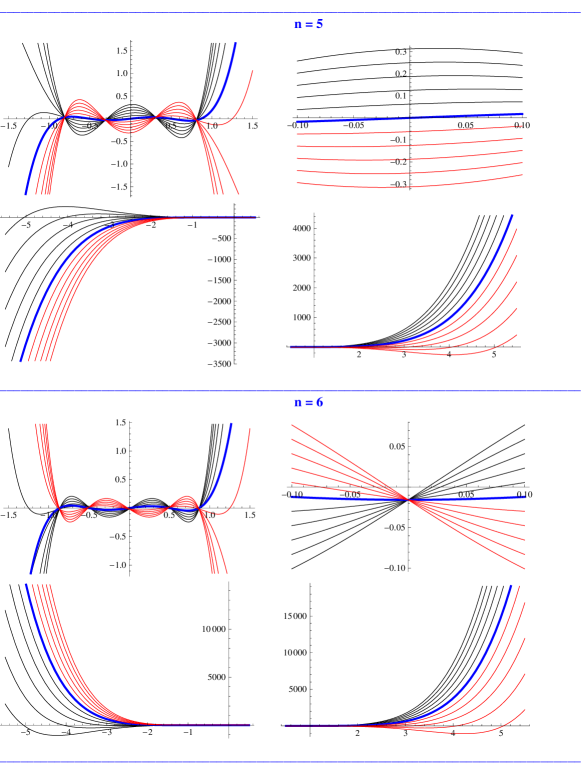
Figure 3: Some perturbed of order 0 by translation with negative parameters $μ˙0=-5(1)-1$ (in black), positive parameters $μ˙0=1(1)5$ (in red) of Chebyshev polynomials of second kind (in bleu) of degrees $n=$ $5$, $6$.

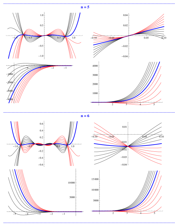
Figure 4: Some perturbed of order 1 by translation with negative parameters $μ˙0=-5(1)-1$ (in black), positive parameters $μ˙0=1(1)5$ (in red) of Chebyshev polynomials of second kind (in bleu) of degrees $n=$ $5$, $6$.

%%%%%%%%%%%%%%%%%%%%%%%%%%%%%%%%%%%%%%%%%%%%%% %%%%%%%%%%%%%%%%%%%%%%%%%%%%%%%%%%%%%%%%%%%%%% %%%%%%%%%%%%%%%%%%%%%%%%%%%%%%%%%%%%%%%%%%%%%%

%

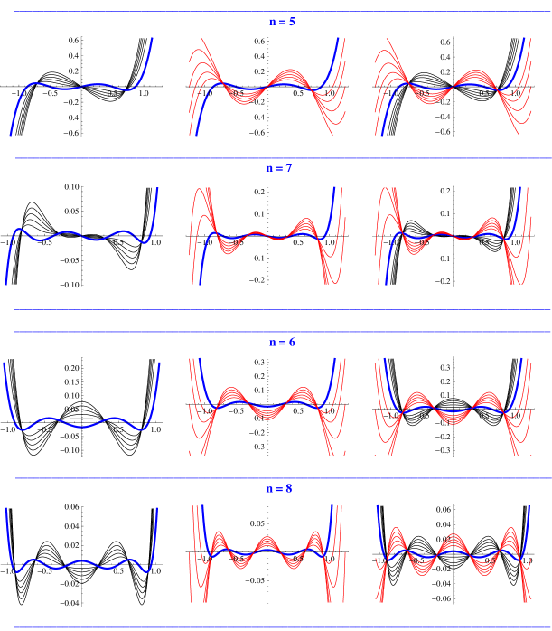
Figure 5: Some perturbed of order 1 by dilatation with parameters $λ˙1=-5(1)-1 ¡ 1$ (in black) and $λ˙1=3(1)7  ¿ 1$ (in red) of Chebyshev polynomials of second kind (in bleu) of degrees $n=$ $5$, $7$, $6$ and $8$.

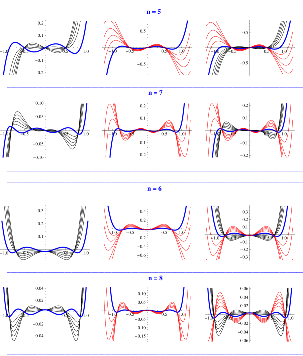
Figure 6: Some perturbed of order 2 by dilatation with parameters $λ˙2=-5(1)-1 ¡ 1$ (in black) and $λ˙2=3(1)7   ¿ 1$ (in red) of Chebyshev polynomials of second kind (in bleu) of degrees $n=$ $5$, $7$, $6$, $8$.

%%%%%%%%%%%%%%%%%%%%%%%%%%%%%%%%%%%%%%%%%%%%%% %%%%%%%%%%%%%%%%%%%%%%%%%%%%%%%%%%%%%%%%%%%%%% %%%%%%%%%%%%%%%%%%%%%%%%%%%%%%%%%%%%%%%%%%%%%% %

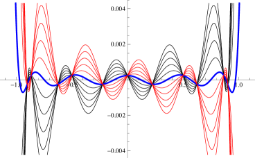
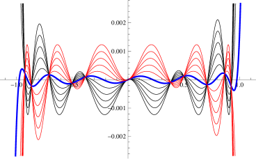
Figure 7: Some perturbed of order 5 by translation with parameters $μ’˙5=-5(1)-1 ¡ 0$ (in black) and $μ˙5=1(1)5   ¿ 0$ (in red) of Chebyshev polynomials of second kind (in bleu).

&

$n=12$ & $n=13$

there are no common zeros & 0 is a double common zero

all interception points are simple & other interception points are simple

&

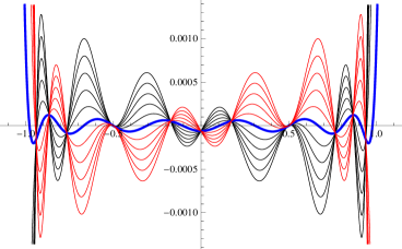
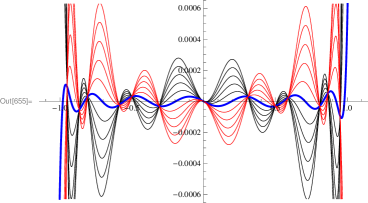
$n=14$ & $n=15$

-0.5 and 0.5 are double common zeros & 0 is a double common zero

other interception points are simple & other interception points are simple

&

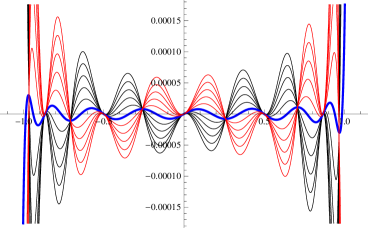
$n=16$ & $n=17$

there are no common zeros & 5 double common zeros

all interception points are simple & all zeros of $P˙5(x)$ are d. common zeros

The zeros of $P˙5(x)$ are $-32≈-0.87, -12, 0,  12 , 32≈0.87.$ %$P˙5(x)=0 ⟺x≈-0.87 V  x=-0.5 V  x=0  V  x=0.5  V x≈0.87$

%

%%%%%%%%%%%%%%%%%%%%%%%%%%%%%%%%%%%%%%%%%%%%%% %%%%%%%%%%%%%%%%%%%%%%%%%%%%%%%%%%%%%%%%%%%%%% %%%%%%%%%%%%%%%%%%%%%%%%%%%%%%%%%%%%%%%%%%%%%%

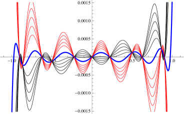
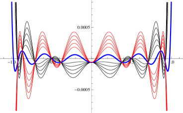
Figure 8: Some perturbed of order 6 by dilatation with parameters $λ’˙6=-5(1)-1 ¡ 1$ (in black) and $λ˙6=3(1)7   ¿ 1$ (in red) of Chebyshev polynomials of second kind (in bleu).

&

$n=13$ & $n=14$ ; 2 simple common zeros

5 simple common zeros & 0 is a double interception point

all interception points are simple & other interception points are simple

&

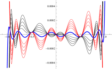
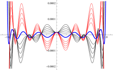
$n=15$; 0 is a simple common zero & $n=16$; no common zeros

-0.5 and 0.5 are double inter. p. & 0 is a double interception point

other interception points are simple & other interception points are simple

&

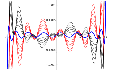
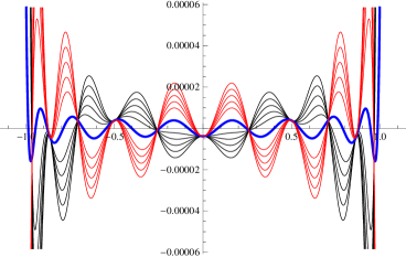
$n=17$; 5 simple common zeros & $n=18$; no common zeros

all interception points are simple & all zeros of $P˙5(x)$ are double inter. p.

The zeros of $P˙5(x)$ are $-32≈-0.87, -12, 0,  12 , 32≈0.87.$ %$P˙5(x)=0 ⟺x≈-0.87 V  x=-0.5 V  x=0  V  x=0.5  V x≈0.87$

%

%%%%%%%%%%%%%%%%%%%%%%%%%%%%%%%%%%%%%%%%%%%%%% %%%%%%%%%%%%%%%%%%%%%%%%%%%%%%%%%%%%%%%%%%%%%% %%%%%%%%%%%%%%%%%%%%%%%%%%%%%%%%%%%%%%%%%%%%%%

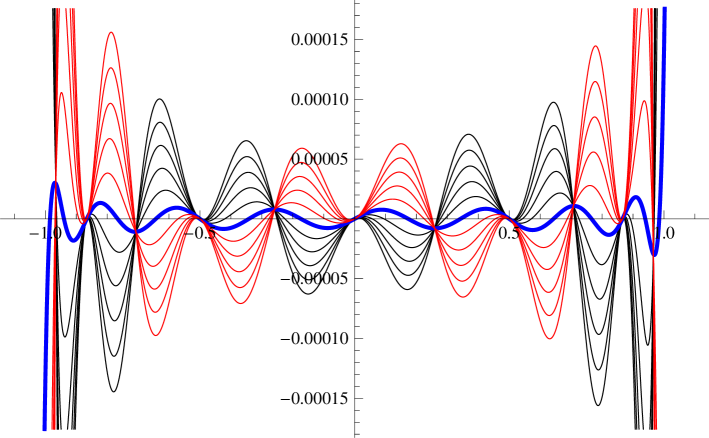
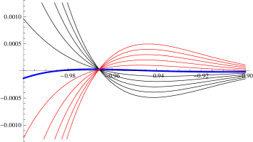
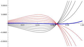
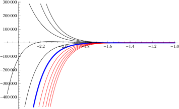
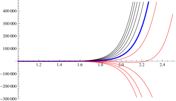
Figure 9: Some perturbed of order 5 by translation with negative parameters $μ’˙5=-5(1)-1 ¡ 0$ (in black) and positive parameters, $μ˙5=1(1)5¿ 0$ (in red) of Chebyshev polynomials of second kind (in bleu) of degree $n=17$. All zeros of $P˙5(x)$ ($-32≈-0.87, -12, 0,  12 , 32≈0.87$) are double common zeros % interception points of $P^t˙17(μ’˙5;5)(x)$, $P^t˙17(μ˙5;5)(x)$ and $P˙17(x)$. There are 11 distinct interception points. There is a zero of $P^t˙17(μ’˙5;5)(x)$ on the left of -1. There is a zero of $P^t˙17(μ˙5;5)(x)$ on the right of 1. Other zeros are in $[-1,1]$. All zeros are real and simple. Polynomials are not symmetric.

&

&

%

%%%%%%%%%%%%%%%%%%%%%%%%%%%%%%%%%%%%%%%%%%%%%% %%%%%%%%%%%%%%%%%%%%%%%%%%%%%%%%%%%%%%%%%%%%%% %%%%%%%%%%%%%%%%%%%%%%%%%%%%%%%%%%%%%%%%%%%%%%

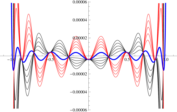
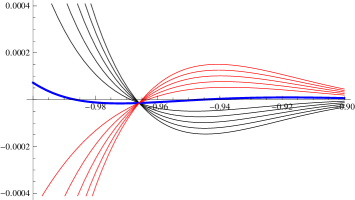
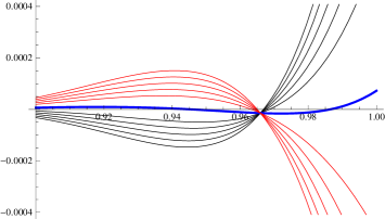
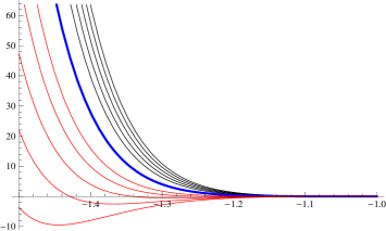
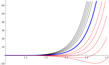
Figure 10: Some perturbed of order 6 by dilatation with parameters $λ’˙6=-5(1)-1 ¡ 1$ (in black) and $λ˙6=3(1)7   ¿ 1$ (in red) of Chebyshev polynomials of second kind (in bleu) of degree $n=18$. All zeros of $P˙5(x)$ ($-32≈-0.87, -12, 0,  12 , 32≈0.87$) are double interception points of $P^d˙18(λ’˙6;6)(x)$, $P^d˙18(λ˙6;6)(x)$ and $P˙18(x)$. There are no common zeros. There are 11 distinct interception points. $P^d˙18(λ’˙6;6)(x)$ has 6 real zeros in $[-1,1]$ and it has 6 pairs of complex conjugate zeros. $P^d˙18(λ˙6;6)(x)$ has 16 real zeros in $[-1,1]$, it has a zero on the left of -1 and a zero on the right of 1. Polynomials and zeros are symmetric.

&

&

%

References

- [1] Abd-Elhameed, W.M., Youssri, Y.H., El-Sissi, N., New hypergeometric connection formulae between Fibonnaci and Chebyshev polynomials, Ramanujan J., pp. 1-15, 2015.
- [2] G. E. Andrews, R. Askey, R. Roy, Special Functions, Cambridge University Press, 71, 1999.
- [3] I. Area, E. Godoy, J. Rodal, A. Ronveaux, A. Zarzo, Bivariate Krawtchouk polynomials: Inversion and connection problems with the NAVIMA algorithm, J. Comput. Appl. Math., 284 (2015) 50-57.
- [4] D. Beghdadi, P. Maroni. Second degree classical forms, Indag. Math., (N.S.) 8(4) (1997), 439-452.
- [5] I. Ben Salah, On the extended connection coefficients between two orthogonal polynomial sequences, Integral Transforms Spec. Funct. 26 (11) (2015), 872-884.
- [6] K. Castillo, F. Marcellán, J. Rivero, On co-polynomials on the real line, J. Math. Anal. App., (2015) 427(1) 469-483.
- [7] K. Castillo, Monotonicity of zeros for a class of polynomials including hypergeometric polynomials, Appl. Math. Comp., 266 (2015) 183-193.
- [8] H. Chagarra, W. Koepf, On linearization and connection coefficients for generalized Hermite polynomials. J. Comput. Appl. Math., 236 (1) (2011) 65-73.
- [9] T. S. Chihara, On co-recursive orthogonal polynomials, Proc. Amer. Math. Soc. 8 (1957) 899-905.
- [10] T. S. Chihara, An Introduction to Orthogonal Polynomials, Mathematics and its Applications, Vol. 13. Gordon and Breach Science Publishers, New York- London-Paris, 1978.
- [11] L. Comptet, Advanced Combinatorics. The Art of Finite and Infinite Expansions, D. Reidel Pub. Comp., Dordrecht, Holand, 1975.
- [12] Z. da Rocha, A general method for deriving some semi-classical properties of perturbed second degree forms: the case of the Chebyshev form of second kind. J. Comput. Appl. Math., 296 (2016) 677-689.
- [13] Z. da Rocha, On the second order differential equation satisfied by perturbed Chebyshev polynomials, J. Math. Anal., 7(1) (2016) 53-69.
- [14] J. Dini, Sur les formes linéaires et les polynômes de Laguerre-Hahn. Thése de doctorat. Univ. P. et M. Curie, Paris VI (1988).
- [15] J. Dini, P. Maroni, A. Ronveaux, Sur une perturbation de la récurrence verifiée par une suite de polynômes orthogonaux. (French) [A perturbation of the recurrence relation satisfied by a sequence of orthogonal polynomials] Portugal. Math. 46 (1989), 269-282.
- [16] J. Dougall, A theorem of Sonine in Bessel functions, with two extentions to spherical hamonics. Proc. Edinb. Math. Soc., 37:33-47, 1919.
- [17] W. Erb, Accelerated Landweber methods based on co-dilated orthogonal polynomials, Numer Algor (2015) 68: 229-260.
- [18] M. Foupouagnigni, W. Koepf, A. Ronveaux, Factorization of the fourth-order differential equation for perturbed classical orthogonal polynomials, J. Comput. Appl. Math., 162 (2004), 299–326.
- [19] J. A. Fromme, M. A. Golberg, Convergence and stability of a collocation method for the generalized airfoil equation, Appl. Math. Comput. 8 (1981) 281–292.
- [20] M. Foupouagnigni,W. Koepf, D.D. Tcheutia, Connection and linearization coefficients of the Askey-Wilson polynomials, J. Symb. Comput. 53, 96-118 (2013).
- [21] W. Gautschi, On mean convergence of extended Lagrange interpolation, J. Comput. Appl. Math., 43 (1992), 19-35.
- [22] W. Gautschi: Orthogonal Polynomials: Computation and Approximation. Numerical Mathematics and Scientific Computation. Oxford Science Publications. Oxford University Press, New York (2004).
- [23] G.H. Golub, C.F. Van Loan, Matrix Computations, The Johns Hopkins University, 1996.
- [24] E. Godoy, I. Area, A. Ronveaux, A. Zarzo, Minimal recurrence relations for connection coefficients between classical orthogonal polynomials: continuous case. J. Comput. Appl. Math., 84 (2) (1997) 257-275.
- [25] E. K. Ifantis, P. D. Siafarikas: Perturbation of the coefficients in the recurrence relation of a class of polynomials, J. Comput. Appl. Math. 57, 163–170 (1995).
- [26] M. Ismail, D. R. Masson, J. Letessier and G. Valent, Birth and death processes and orthogonal polynomials, in: P. Nevai, Ed., Orthogonal Polynomials: Theory and Pratice (Kluver, Dordrecht, 1990) 229–255.
- [27] M. E. Ismail, Classical and Quantum Orthogonal Polynomials in One Variable. Encyclopedia of Mathematics and its Applications, 98. Cambridge University Press, Cambridge, 2005.
- [28] E. Leopold, The extremal zeros of a perturbed orthogonal polynomials systems, J. Comp. Appl. Math., 98 (1998) 99-120.
- [29] J. Letessier, Some results on co-recursive associated Laguerre and Jacobi polynomials, SIAM J. Math. Anal. 25 (1994) 528–548.
- [30] S. Lewanowicz, Recurrence relations for the connection coefficients of orthogonal polynomials of a discrete variable, J. Comput. Appl. Math., 76 (1996) 213-229.
- [31] W. Koepf, D. Schmersau, Representations of orthogonal polynomials, J. Comput. Appl. Math. 90, 1998, 57-94.
- [32] F. Marcellán, J.S. Dehesa and A. Ronveaux, On orthogonal polynomials with perturbed recurrence relations, J. Comput. Appl. Math. 30 (1990) 203–212.
- [33] P. Maroni, Le calcul des formes linéaires et les polynômes orthogonaux semi-classiques. (French) [Calculation of linear forms and semiclassical orthogonal polynomials] Lecture Notes in Math., 1329 (1988), 279–290.
- [34] P. Maroni, Sur la suite de polynômes orthogonaux associé à la forme (in French) [On the sequence of orthogonal polynomials associated with the form ], Period. Math. Hung. 21 (1990) 223-248.
- [35] P. Maroni, Une théorie algébrique des polynômes orthogonaux. Application aux polynômes orthogonaux semi-classiques (in French) [An algebraic theory of orthogonal polynomials. Applications to semi–classical orthogonal polynomials]. In C. Brezinski et al. Eds., Orthogonal Polynomials and their Applications (Erice, 1990), IMACS Ann. Comput. Appl. Math., 9, Baltzer, Basel, (1991), 95-130.
- [36] P. Maroni, Variations around classical orthogonal polynomials. Connected problems, J. Comput. Appl. Math., 48, 133-155, 1993.
- [37] P. Maroni, Fonctions eulériennes. Polynômes orthogonaux classiques. Techniques de l’Ingénieur, traité Généralités (Sciences Fondamentales), 1994.
- [38] P. Maroni, An introduction to second degree forms, Adv. Comput. Math., 3 (1995), 59-88.
- [39] P. Maroni, Tchebychev forms and their perturbed as second degree forms, Ann. Numer. Math., 2 (1-4) (1995), 123–143.
- [40] P. Maroni, M. I. Tounsi, The second–order self associated orthogonal sequences, J. Appl. Math., 2004:2 (2004) 137-167.
- [41] P. Maroni, M. Mejri, Some perturbed sequences of order one of the Chebyshev polynomials of second kind, Integral Transforms Spec. Funct. 25 (1) (2014), 44-60.
- [42] P. Maroni, Z. da Rocha, Connection coefficients between orthogonal polynomials and the canonical sequence: an approach based on symbolic computation, Numer. Algorithms, 47-3 (2008) 291-314.
- [43] P. Maroni, Z. da Rocha, Connection coefficients for orthogonal polynomials: symbolic computations, verifications and demonstrations in the Mathematica language, Numer. Algor., 63-3 (2013) 507-520.
- [44] P. Maroni, Z. da Rocha, Software CCOP - Connection Coefficients for Orthogonal Polynomials, Numer. Algor., (2013), http://www.netlib.org/numeralgo/, na34 package.
- [45] P. Maroni, Z. da Rocha, Software CCOP - TUTORIAL. Numer. Algor., 40 p. (2013), http://www.netlib.org/numeralgo/, na34 package.
- [46] J. C. Mason, D. C. Handscomb, Chebyshev Polynomials, Chapman & Hall/CRC, Boca Raton, FL, 2003.
- [47] F. Peherstorfer, Finite perturbations of orthogonal polynomials, J. Comput. Appl. Math. 44 (1992) 275–302.
- [48] J. Riordan, An Introduction to Combinatorial Analysis. Dover, 1958.
- [49] J. Riordan, Combinatorial Identities, John Willey and Sons, Inc., 1968.
- [50] J. Riordan, Introduction to Combinatorial Analysis, Dover ed., N.Y., 2002.
- [51] A. Ronveaux, S. Belmehdi, J. Dini, P. Maroni, Fourth-order differential equation for the co-modified semi-classical orthogonal polynomials, J. Comput. Appl. Math., 29 (2) (1990), 225–231.
- [52] A. Ronveaux, A. Zargi, E. Godoy, Fourth-order differential equations satisfied by the generalized co-recursive of all classical orthogonal polynomials. A study of their distribution of zeros, J. Comput. Appl. Math., 59 (1995), 295-328.
- [53] G. Sansigre, G. Valent, A large family of semi–classical polynomials: the perturbed Tchebychev, J. Comput. Appl. Math., 57 (1995), 271-281.
- [54] G. Szegö, Orthogonal Polynomials, fourth edition, Amer. Math. Soc., Colloq. Publ., vol. 23, Providence, Rhode Island, 1975.
- [55] H.A. Slim, On co-recursive orthogonal polynomials and their application to potential scattering, J. Math. Anal. Appl. 136 (1988) 1-19.
- [56] M. Foupouagnigni, W. Koepf, D. D. Tcheutia. Connection and linearization coefficients of the Askey-Wilson polynomials. J. Symbolic Comput., 53:96-118, 2013b.
- [57] D. D. Tcheutia, On Connection, Linearization and Duplication Coefficients of Classical Orthogonal Polynomials. PhD thesis, Universität Kassel (2014). https://kobra.bibliothek.uni-kassel.de/handle/urn:nbn:de:hebis:34-2014071645714
- [58] Weisstein, Eric W. ”Vieta’s Formulas.” From MathWorld–A Wolfram Web Resource. ttp://mathworld.wolfram.com/VietasFormulas.html
- [59] A. Zhedanov, Rational spectral transformations and orthogonal polynomials, J. Comput. Appl. Math., 85 (1997), 67–86.
%%%%%%%%%%%%%%%%%%%%%%%%%%%%%%%%%%%%%%%%%% %
%
%%%%%%%%%%%%%%%%%%%%%%%%%%%%%%%%%%%%%%%%%%%%% %%%%%%%%%%%%%%%%%%%%%%%%%%%%%%%%%%%%%%%%%%%%%
%%%%%%%%%%%%%%%%%%%%%%%%%%%%%%%%%%%%%%%%%%%%%%% %
%%%%%%%%%%%%%%%%%%%%%%%%%%%%%%%%%%%%%%%%%%%%%% %%%%%%%%%%%%%%%%%%%%%%%%%%%%%%%%%%%%%%%%%%%%%% %%%%%%%%%%%%%%%%%%%%%%%%%%%%%%%%%%%%%%%%%%%%%%
%
%%%%%%%%%%%%%%%%%%%%%%%%%%%%%%%%%%%%%%%%%%%%%% %%%%%%%%%%%%%%%%%%%%%%%%%%%%%%%%%%%%%%%%%%%%%% %%%%%%%%%%%%%%%%%%%%%%%%%%%%%%%%%%%%%%%%%%%%%% %
& &