Quantum versus classical effects at zero and finite temperature in the quantum pyrochlore Yb₂Ti₂O₇

We study the finite temperature properties of the candidate quantum spin ice material Yb₂Ti₂O₇ within the framework of an anisotropic nearest-neighbor spin $1/2$ model on the pyrochlore lattice. Using a combination of finite temperature Lanczos and classical Monte Carlo methods, we highlight the importance of quantum mechanical effects for establishing the existence and location of the low-temperature ordering transition. We perform simulations of the $32$ site cluster, which capture the essential features of the specific heat curve seen in the cleanest known samples of this material. Focusing on recent experimental findings [A. Scheie et al., Phys. Rev. Lett. 119, 127201 (2017) and J. D. Thompson et al., Phys. Rev. Lett. 119, 057203 (2017)], we then address the question of how the phase boundary between the ferromagnetic and paramagnetic phases changes when subjected to a magnetic field. We find that the quantum calculations explain discrepancies observed with a completely classical treatment and show that Yb₂Ti₂O₇ displays significant renormalization effects, which are at the heart of its reentrant lobed phase diagram. Finally, we develop a qualitative understanding of the existence of a ferromagnet by relating it to its counterpart that exists in the vicinity of the classical ice manifold.

Introduction— Frustrated magnets constitute a fertile hunting ground for discovering unconventional states of matter, including spin liquids with topological properties. The presence of multiple competing energy scales is at the heart of several contentious issues - ranging from the precise knowledge of the low-energy effective Hamiltonian to the reliable determination of the low-energy properties. While spin liquids are desirable, "order-by-disorder" effects Henley (1989); Villain et al. (1980) typically dominate leading to magnetically ordered or valence bond states. However, combined experimental and theoretical efforts determined Hamiltonian parameters for Yb₂Ti₂O₇ (YbTO) Ross et al. (2011); Savary and Balents (2012); Bloete et al. (1969), and suggested a quantum spin ice (spin liquid) ground state Hermele et al. (2004), possibly circumventing the issues above. This phase is qualitatively described as a quantum superposition of configurations in which the spins are constrained to point into or out of tetrahedra of the pyrochlore lattice, with a two-in-two-out "ice rule" Bernal and Fowler (1933); Ramirez et al. (1999); Bramwell and Gingras (2001), a schematic of one such configuration is depicted in Fig. 1. Defects (spin flips) in this rule produce a pair of magnetic "monopoles"; the analogy with electrodynamics led to the theoretical prediction of exotic gapless excitations or "photons" Hermele et al. (2004). This fuelled several other studies Pan et al. (2014); Wan and Tchernyshyov (2012); Applegate et al. (2012); Robert et al. (2015); Jaubert et al. (2015) to understand the true nature of YbTO.

Real materials always have some disorder; thus it is important to clarify the nature of the ground state theoretically. Multiple works have addressed the issue at the classical level Yan et al. (2017); Jaubert et al. (2015); Robert et al. (2015); Scheie et al. (2017), but quantum treatments have been limited to mean field theories Chang et al. (2012), small clusters Onoda and Tanaka (2011); Jaubert et al. (2015), high temperature approaches Hayre et al. (2013); Applegate et al. (2012); Jaubert et al. (2015) or sign problem free parameter sets Shannon et al. (2012); Kato and Onoda (2015); the latter may not represent YbTO.

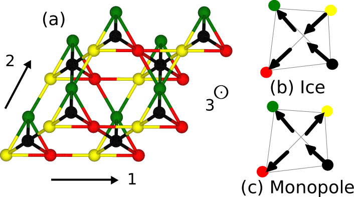
Figure 1: (a) $32$ site unit cell of the pyrochlore lattice used for the calculations in the paper, as viewed along the global [111] direction with periodic boundary conditions along the $1$,$2$ and $3$ directions. The four colors represent the four FCC sublattices. (b) and (c) show representative configurations of four spins on a single tetrahedron (b) satisfying the two-in two-out ice rule and (c) a monopole associated with a defect in the local ice rule.

Here we show, numerically, that quantum calculations of YbTO favor the picture of a ferromagnet (FM) at low temperature. Using the finite temperature Lanczos method (FTLM) Jaklic and Prelovsek (1994); Prelovsek and Bonca (2013), on an effective spin 1/2 anisotropic model on the pyrochlore lattice, we find good agreement with the experimentally observed Schottky anomaly centered at $2.4$ K, and the approximate location of the transition at low temperature Thompson et al. (2017); Scheie et al. (2017); Arpino et al. (2017); Pe çanha Antonio et al. (2017). Our approach complements previous reports Applegate et al. (2012); Hayre et al. (2013) on YbTO with the numerical linked cluster (NLC) method. In addition, our calculations in a [111] magnetic field indicate that YbTO has substantial magnetization at small field strengths.

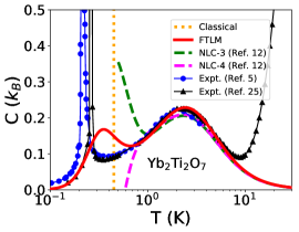
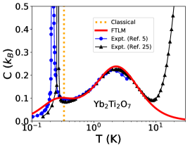
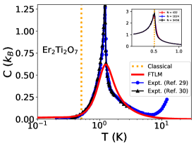
Figure 2: (Color online): Heat capacity (per mole of the magnetic ion) of Yb₂Ti₂O₇ and Er₂Ti₂O₇ in units of the Boltzmann constant ($k_{B}$) as a function of temperature. The theoretical FTLM calculations on the $32$ site cluster used model parameters from Ref. Ross et al. (2011) and Ref. Thompson et al. (2017) for Yb₂Ti₂O₇ (left and central panels respectively) and Ref. Savary et al. (2012) for Er₂Ti₂O₇ (right panel). For comparison, results from experimental data sets Bloete et al. (1969); Arpino et al. (2017); Dalmas de Réotier et al. (2012); Niven et al. (2014) and previous NLC calculations Applegate et al. (2012) are shown. The classical estimates of $T_{c}$ are obtained with classical Monte Carlo, and the results of the profile for Er₂Ti₂O₇ are shown in the inset.

We discuss three main results. First, we demonstrate that quantum effects are crucial for the finite temperature properties of YbTO even for temperatures greater than the ordering temperature $T_{c}$; frustrated interactions and quantum effects renormalize $T_{c}$ significantly. This complexity is manifest in a magnetic field, and responsible for its unusual reentrant lobed phase diagram Scheie et al. (2017), thus, an explanation of recent experiments Scheie et al. (2017); Thompson et al. (2017); Pe çanha Antonio et al. (2017) constitute the second purpose of this study. Finally, we present a simple picture in parameter space connecting the ice manifold to the YbTO parameter set, suggesting that the FM obtained within perturbation theory is connected to its counterpart in the non-perturbative regime. For these purposes, we have carried out simulations on $32$ sites as in Fig. 1(a), with a Hilbert space per momentum sector of approximately $536$ million, significantly larger than previous quantum treatments Onoda and Tanaka (2011); Jaubert et al. (2015) on the same model.

The relevant effective spin Hamiltonian including the nearest neighbor interactions and onsite Zeeman coupling to an external magnetic field ($h=(h_{x},h_{y},h_{z})$) is Curnoe (2007); Onoda (2011); Ross et al. (2011),

$$H=\frac{1}{2}\sum_{ij}J^{\mu\nu}_{ij}S^{\mu}_{i}S^{\nu}_{j}-\mu_{B}h^{\mu}\sum_{i}g^{\mu\nu}_{i}S^{\nu}_{i}$$ (1)

where $i,j$ are nearest neighbors and $\mu,\nu$ refer to $x,y,z$, $S^{\mu}_{i}$ refer to the spin $1/2$ components at site $i$, and $\bf{J_{ij}}$ and $\bf{g_{i}}$ are bond and site dependent interaction and coupling matrices respectively, the former characterized completely by four and the latter by two independent parameters. The interaction part is most illuminating when written in terms of spin directions along the local [111] axes (denoted by ${\mathcal{S}}$),

$$H_{int} = \sum_{\langle i,j\rangle}(2-\lambda)J_{zz}\;\;{\mathcal{S}}^{z}_{i}{\mathcal{S}}^{z}_{j}-\lambda J_{\pm}\Big{(}{\mathcal{S}}^{+}_{i}{\mathcal{S}}^{-}_{j}+{\mathcal{S}}^{-}_{i}{\mathcal{S}}^{+}_{j}\Big{)}$$ (2)

$$+\lambda J_{\pm\pm}\;\;\Big{(}\gamma_{ij}{\mathcal{S}}^{+}_{i}{\mathcal{S}}^{+}_{j}+\gamma^{*}_{ij}{\mathcal{S}}^{-}_{i}{\mathcal{S}}^{-}_{j}\Big{)}$$

$$+\lambda J_{z,\pm}\;\;\Big{[}{\mathcal{S}}^{z}_{i}\Big{(}{\mathcal{S}}^{+}_{j}\zeta_{ij}+{\mathcal{S}}^{-}_{j}\zeta^{*}_{ij}\Big{)}+i\leftrightarrow j\Big{]}$$

where $J_{zz},J_{\pm},J_{\pm\pm},J_{z,\pm}$ are couplings and the parameter $\lambda$ has been introduced to tune from the classical ice manifold ($\lambda=0$) to material-relevant parameters ($\lambda=1$). $\gamma_{ij}$ and $\zeta_{ij}$ are bond dependent phases, the corresponding $4\times 4$ matrices have been written out in the supplementary information. We work with $\lambda=1$, unless otherwise noted.

Classical versus quantum effects on the specific heat capacity in zero field— We now discuss the results of the temperature dependence of the specific heat of YbTO in zero field using FTLM. This Krylov space method constructs an effective Hamiltonian in the space of suitably chosen vectors (powers of $H$ on a random vector) and calculates observables (that commute with $H$) from it. The efficiency of FTLM crucially depends on the adequacy of a small number of powers of the Hamiltonian ($M$) and a small number of starting random vectors ($R$) Jaklic and Prelovsek (1994); Prelovsek and Bonca (2013); Hanebaum and Schnack (2014). Some details of the method and its convergence properties are discussed in the supplement.

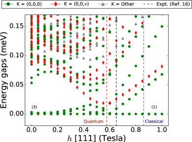
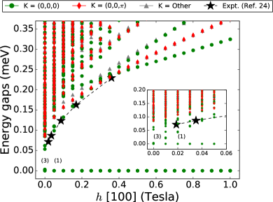
Figure 3: (Color online): Energy (relative to the ground state) versus magnetic field ($h$) in [111] (left) and [100] (right) directions plotted by momentum sector ($k_{1}$,$k_{2}$,$k_{3}$). $M=400$ iterations were used for ${\bf k}=(0,0,0)$ and ${\bf k}=(0,0,\pi)$ and $M=200$ for the other sectors (denoted by $\bf k=$ other). $k_{1}$ and $k_{2}$ directions correspond to translations perpendicular to [111] and the $k_{3}$ direction corresponds to translations along [111]. The dashed lines indicate the classical, quantum and experimental estimates of the critical field at zero temperature. There is no phase transition for the [100] direction, although there is reorganization of the energy levels at small fields (inset). The experimental field dependent gap is also shown for the [100] case. For both cases, the quasidegeneracies of the ground state are shown in parentheses.

The leftmost panel of Fig. 2 shows the converged specific heat profile (for the parameters of Ref. Ross et al. (2011)) across a wide range of temperatures for $M=100$ and $R=160$, along with two experimental data sets Arpino et al. (2017); Bloete et al. (1969). The agreement with the NLC approach at high temperatures is excellent, which serves as a check of our calculations. Importantly, the quantum treatment yields a small "peak" ($T_{c}\approx 0.34$ K), which appears as a crossover, but is not accessible in the NLC approach Applegate et al. (2012). When compared to classical Monte Carlo (MC) simulations, which yield $T_{c}\approx 0.45$ K, we conclude that $T_{c}$ is renormalized due to quantum effects ($0.11$ K is not a small scale for the phenomenon relevant to experiments, as will become clear shortly). Based on finite size analyses (of the MC calculations), the extent of the change in $T_{c}$ on approaching the thermodynamic limit (TDL) is insufficient to reconcile the classical and quantum estimates.

Prominently, the Schottky anomaly at $2.4$ K highlights the importance of quantum effects, since it is completely absent from classical simulations in zero field. The agreement of this feature with experiments is remarkable; the deviations are small and not visualized on the scale of the plot. Even below $T_{c}$, the numerically computed values essentially lie on top of the experimental data. Above 10 K the experimental data includes contributions from non-magnetic degrees of freedom, not part of the model Hamiltonian.

Recently, different parameters (with reduced $J_{zz}$) have been reported by Ref. Thompson et al. (2017); the central panel of Fig. 2 shows our results for this set. The Schottky anomaly is explained well here too, but importantly a lower $T_{c}$ is observed, both classically and quantum mechanically; the latter appears as a broad hump at $T_{c}\approx 0.27$ K. This suggests longer correlation lengths leading to more pronounced finite size effects and YbTO’s possible closeness to a phase boundary Jaubert et al. (2015); Robert et al. (2015). However, several aspects of experiments can be understood from the set of Ref. Ross et al. (2011)  (with smaller finite size effects); we use those for the remainder of the paper.

While YbTO is the main focus of this work, we demonstrate the effectiveness of the approach for another pyrochlore, Er₂Ti₂O₇ (ErTO). ErTO is a candidate for the "order by disorder effect" Henley (1989); Villain et al. (1980) and has been extensively studied Savary et al. (2012); Oitmaa et al. (2013); Zhitomirsky et al. (2012); Hallas et al. (2017). We use the Hamiltonian parameters from Ref. Savary et al. (2012), and compare to two experimental data sets Dalmas de Réotier et al. (2012); Niven et al. (2014), our results are in the rightmost panel of Fig. 2. Unlike YbTO, ErTO displays no prominent Schottky anomaly Hallas et al. (2017), but instead a single phase transition at $T_{c}=1.23\pm 0.01$ K. The quantum calculations capture this effect, and we find $T_{c}\approx 1.26$ K. In contrast, the MC calculations (see inset for profiles for of systems ranging from $432$ to $3456$ sites) show a much lower $T_{c}\approx 0.51(1)$ K.

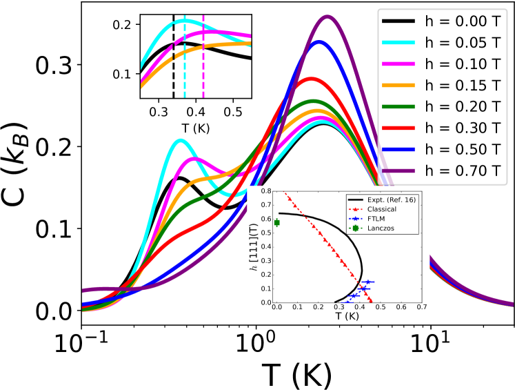
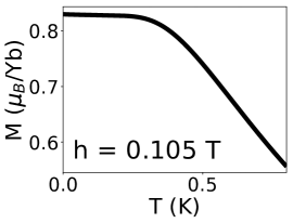
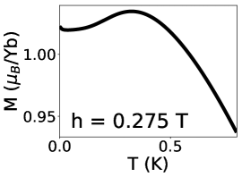
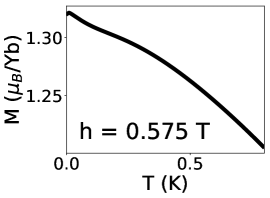
Figure 4: (Color online): The top panel shows the heat capacity (per mole of Yb) in units of the Boltzmann constant ($k_{B}$) as a function of temperature for different [111] magnetic field strengths ($h$). The upper inset zooms in on the low temperature peak; the dashed lines indicate the location of $T_{c}$. (For $h\gtrsim 0.15$T, the peaks are not visible). The lower inset shows the experimental lobed phase diagram and the quantum and classical phase boundaries. The lower panels show the magnetization ($M$) measured along the [111] direction as a function of temperature for various representative $h$.

Low energy spectra and quantum phase transitions in a [111] and [100] magnetic field— The difference between classical and quantum treatments of YbTO is particularly striking at zero temperature, in a [111] magnetic field. Since the Hamiltonian has translational symmetry, all eigenstates have definite momenta ${\bf k}=(k_{1},k_{2},k_{3})$; for the $32$ site cluster each $k_{i}=0$ or $k_{i}=\pi$. The lowest lying energies are mapped out in all $8$ momentum sectors in Fig. 3. Since only momenta ${\bf k}=(0,0,0)$ and ${\bf k}=(0,0,\pi)$ are involved in the zero temperature phase transition, their corresponding labels have been highlighted, the rest are denoted as "${\bf k}=$other".

In zero field there are three quasidegenerate states, all in ${\bf k}=(0,0,0)$ followed by two more states separated by approximately $0.05$ meV. This is at odds with six quasidegenerate states expected of a cubic FM; this can be attributed to the lack of cubic symmetry of the $32$ site cluster and the large splittings between states. An analogous effect involving large tunneling between time reversal symmetric odd and even states is also seen on the kagome Kumar et al. (2016). For finite fields, only three quasidegenerate states in ${\bf k}=(0,0,0)$ remain part of the low energy manifold while the other states separate out from these. (In the TDL, an infinitesimally small [111] field would gap out three of the six states for a cubic FM). Simultaneously, the lowest ${\bf k}=(0,0,\pi)$ state is lowered in energy. Then between $0.55$ to $0.60$ T, the lowest ${\bf k}=(0,0,\pi)$ state makes its closest approach to the quasidegenerate manifold; at this critical field ($h_{c}$), the ${\bf k}=(0,0,0)$ states also split into three branches. The observed $h_{c}$ agrees well with the experimental value ($0.65$ T) Scheie et al. (2017), and is significantly lower than the classical estimate of $0.86(1)$ T.

In contrast, in a [100] field (right panel of Fig. 3), there is no sign of a phase transition, consistent with the findings of Ref. Thompson et al. (2017). At small fields ($<0.03$T), the three quasidegenerate states split (see inset) yielding a single non-degenerate ground state which is qualitatively the same as the high field limit. The trends in the excited eigenenergies also explain the field dependent gap of Ref. Thompson et al. (2017). These observations collectively suggest YbTO is a FM.

Specific heat and magnetization in a [111] magnetic field— It is now natural to ask how quantum fluctuations manifest themselves at finite field and temperature. Recently, Ref. Scheie et al. (2017) found that on increasing the [111] field from $0$ to $0.2$ T, $T_{c}$ increased significantly from $0.27$ K to $0.42$K, before it gradually decreased towards zero for higher fields, yielding a reentrant lobed phase diagram. While this initial increase is expected of a first order phase transition, the magnitude of this effect could not be captured classically.

To address this issue, we performed FTLM calculations in a [111] field $h$; our results are shown in Fig. 4. (As a compromise between accuracy and computer time, we chose $R=40$ and $M=50$). On increasing $h$, the Schottky anomaly increases in height and the associated entropy increases. Quantum mechanically, the combined entropy of the peak ($S_{peak}$) and anomaly must be constant ($\ln(2)$ in units of $k_{B}$, ignoring non-magnetic contributions), implying $S_{peak}$ decreases with increasing $h$. Next, the upper inset of Fig. 4 shows the low temperature peaks, marked by dashed lines, the broad features they are associated with move right by $\approx 0.1$ K. Both observations agree with experimental findings Scheie et al. (2017); the lower inset compares their phase diagram and our simulations.

These inferences are confirmed by the magnetization along the [111] direction ($M$)

$$M(T,h)=k_{B}T\frac{\partial\ln Z(T,h)}{\partial h}$$ (3)

where $Z(T,h)$ is the partition function directly calculated in FTLM. $M(T,h)$ was evaluated using finite differences; $\delta h$ was chosen to be $0.01$ T for small fields, and $0.05$ T for larger fields. Representative results are shown in Fig. 4.

$M$($T\rightarrow 0,h$) is non zero for small $h$ and increases with $h$ suggesting that YbTO is a FM at low temperatures; noting that the distinction between a FM and very good paramagnet (PM) is difficult for a $32$ site system (also see supplement) In addition, the quantum simulations show signs of a phase transition from FM to PM, for example a (smooth) kink is seen in $M(T,h)$ up to $\approx 0.15$ T. Then for intermediate $h$ ($h\approx 0.15$ T to $h\approx 0.5$ T), $M$ in the putative FM phase is lower than that in the PM, which is consistent with $T_{c}$ decreasing with increasing $h$. By $0.55$ T, there is no phase transition, consistent with the zero temperature findings.

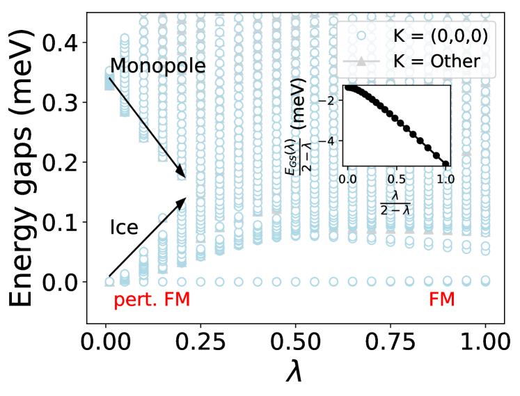
Figure 5: (Color online): Energy (relative to the ground state) versus $\lambda$, the parameter defined in the text, that allows us to tune from the classical ice manifold ($\lambda=0$) to the experimentally relevant parameters ($\lambda=1$). The inset shows the total ground state energy which smoothly evolves from the perturbative to non-perturbative regime.

Relation of YbTO to the ice manifold— We now provide a qualitative interpretation of the existence of an FM by varying $\lambda$ (in Eq. (2)) from $0$ (classical ice) to $1$ (YbTO-relevant parameters) and monitoring the spectrum, our results are shown in Fig. 5. When $\lambda$ is small, perturbative arguments apply due to presence of the gap of order $(2-\lambda)J_{zz}$. The leading order contribution is to second order; the $J_{z\pm}$ term selects the six FM states Ross et al. (2011); Savary and Balents (2012). When $\lambda$ is increased, the energy of the monopole (defect) manifold decreases relative to the highest energy of the ice-like manifold, which itself has split, and around $\lambda\approx 0.25$ the two features meet. However, the ground state is qualitatively unaffected by this high energy feature as the state selection from the ice manifold has already occurred at a much lower energy scale (the inset shows the ground state energy evolving from the perturbative regime to the non-perturbative one). Thus, we suggest that the FM seen in perturbation theory is connected to the FM established earlier in the paper, for the parameters of Ref. Ross et al. (2011). This adiabatic connection suggests YbTO is a near-collinear FM Chang et al. (2012); Yasui et al. (2003).

Conclusion— In summary, quantum mechanical effects are crucial to understanding the zero and finite temperature properties of YbTO. Despite the limitations of finite size ($32$ sites), we observed good agreement between available experimental data and simulations for a wide range of temperatures. In finite [111] fields, we saw a significant increase in $T_{c}$ of $\approx 0.1$ K till $\approx 0.15$ T. The presence of substantial magnetization at small fields suggests YbTO is a FM. This picture is strengthened by connecting our results to those known within second order perturbation theory of the ice manifold.

Finally, we showed the utility of FTLM for large Hilbert spaces, for meaningfully studying certain properties of other pyrochlores at finite temperature, as long as the correlation lengths are sufficiently short. One hopes that recent numerical advances at zero and finite temperature Bruognolo et al. (2017); Claes and Clark (2017); Changlani et al. (2009); Holmes et al. (2016a); Petruzielo et al. (2012); Holmes et al. (2016b); Tubman et al. (2016); Blunt et al. (2015) will push the limits of interesting sizes (of high-dimensional systems) one can go to with some degree of confidence.

Acknowledgements— I thank O. Tchernyshyov and S. Zhang for teaching me the basics of this field of research and for extensive discussions. I gratefully acknowledge C. Broholm, A. Scheie, J. Kindervater, R.R.P. Singh, R. Coldea, M. Gingras, J. Rau, Y. Wan, K. Plumb, S. Säubert, A. Eyal, S. Koohpayeh, L. Jaubert and B. Clark for useful discussions and D. Kochkov for sharing large-scale exact diagonalization tricks. I thank R.R.P. Singh for sharing his NLC data and for critically reading the first draft of this manuscript, B. Gaulin, A. Hallas and J. Gaudet for providing experimental specific heat data sets from their review article, and A. Scheie and K. Arpino for providing data from their published work. This work was supported through the Institute for Quantum Matter at Johns Hopkins University, by the U.S. Department of Energy, Division of Basic Energy Sciences, Grant DE-FG02-08ER46544. I gratefully acknowledge the Johns Hopkins Homewood High Performance Cluster (HHPC) and the Maryland Advanced Research Computing Center (MARCC), funded by the State of Maryland, for computing resources and Yi Li for sharing part of her computer allocation time.

Supplemental Material for "Quantum versus classical effects at zero and finite temperature in the quantum pyrochlore Yb₂Ti₂O₇"

I Low energy effective Hamiltonian

In this section, we discuss details of the relevant spin $1/2$ low-energy effective Hamiltonian on the pyrochlore lattice, with nearest neighbor interactions and Zeeman coupling to an external field ($h=(h_{x},h_{y},h_{z})$) Curnoe (2007); Onoda (2011); Ross et al. (2011),

$$H=\frac{1}{2}\sum_{ij}J^{\mu\nu}_{ij}S^{\mu}_{i}S^{\nu}_{j}-\mu_{B}h^{\mu}\sum_{i}g^{\mu\nu}_{i}S^{\nu}_{i}$$ (S1)

where $i,j$ are nearest neighbors and $\mu,\nu$ refer to $x,y,z$, $S^{\mu}_{i}$ refer to the spin components at site $i$, and $\bf{J}_{ij}$ and $\bf{g}_{i}$ are bond and site dependent interactions and coupling matrices respectively (whose components have been written out in Eq. S1). The pyrochlore lattice has four sublattices which we label as $0,1,2,3$ and we take the relative locations of the sites on a single tetrahedron to be, (in units of lattice constant $a$) ${\bf{r}_{0}}=(1/8,1/8,1/8)$, ${\bf{r}_{1}}=(1/8,-1/8,-1/8)$, ${\bf{r}_{2}}=(-1/8,1/8,-1/8)$ and ${\bf{r}_{3}}=(-1/8,-1/8,1/8)$. Symmetry considerations dictate that $\bf{J}_{ij}$ and $\bf{g}_{i}$ are completely described by four and two scalars respectively. $\bf{J}_{ij}$ depends only on the sublattices that $i,j$ belong to (similarly $\bf{g}_{i}$ depends only on the sublattice of site $i$), and thus we use the notation in terms of $i,j=0,1,2,3$. Also, since $\bf{J}_{ij}=\bf{J}_{ji}^{T}$, only the $i<j$ matrices are written out. The $\bf{J}_{ij}$ matrices are,

$$\bf{J}_{01}\equiv\left(\begin{array}[]{ccc}J_{2}&J_{4}&J_{4}\\ -J_{4}&J_{1}&J_{3}\\ -J_{4}&J_{3}&J_{1}\end{array}\right)\bf{J}_{02}\equiv\left(\begin{array}[]{ccc}J_{1}&-J_{4}&J_{3}\\ J_{4}&J_{2}&J_{4}\\ J_{3}&-J_{4}&J_{1}\end{array}\right)$$

$$\bf{J}_{03}\equiv\left(\begin{array}[]{ccc}J_{1}&J_{3}&-J_{4}\\ J_{3}&J_{1}&-J_{4}\\ J_{4}&J_{4}&J_{2}\end{array}\right)\bf{J}_{12}\equiv\left(\begin{array}[]{ccc}J_{1}&-J_{3}&J_{4}\\ -J_{3}&J_{1}&-J_{4}\\ -J_{4}&J_{4}&J_{2}\end{array}\right)$$

$$\bf{J}_{13}\equiv\left(\begin{array}[]{ccc}J_{1}&J_{4}&-J_{3}\\ -J_{4}&J_{2}&J_{4}\\ -J_{3}&-J_{4}&J_{1}\end{array}\right)\bf{J}_{23}\equiv\left(\begin{array}[]{ccc}J_{2}&-J_{4}&J_{4}\\ J_{4}&J_{1}&-J_{3}\\ -J_{4}&-J_{3}&J_{1}\end{array}\right)$$ (S2)

Defining $g_{+}=\frac{1}{3}(2g_{xy}+g_{z})$ and $g_{-}=\frac{1}{3}(g_{xy}-g_{z})$, the $\bf{g}_{i}$ matrices read as,

$$\bf{g}_{0}\equiv\left(\begin{array}[]{ccc}g_{+}&-g_{-}&-g_{-}\\ -g_{-}&g_{+}&-g_{-}\\ -g_{-}&-g_{-}&g_{+}\end{array}\right)\bf{g}_{1}\equiv\left(\begin{array}[]{ccc}g_{+}&g_{-}&g_{-}\\ g_{-}&g_{+}&-g_{-}\\ g_{-}&-g_{-}&g_{+}\end{array}\right)$$

$$\bf{g}_{2}\equiv\left(\begin{array}[]{ccc}g_{+}&g_{-}&-g_{-}\\ g_{-}&g_{+}&g_{-}\\ -g_{-}&g_{-}&g_{+}\end{array}\right)\bf{g}_{3}\equiv\left(\begin{array}[]{ccc}g_{+}&-g_{-}&g_{-}\\ -g_{-}&g_{+}&g_{-}\\ g_{-}&g_{-}&g_{+}\end{array}\right)$$ (S3)

The interaction part when written in terms of spin directions along the local [111] axes (denoted by ${\mathcal{S}}$), is,

$$H_{int} = \sum_{\langle i,j\rangle}(2-\lambda)J_{zz}\;\;{\mathcal{S}}^{z}_{i}{\mathcal{S}}^{z}_{j}-\lambda J_{\pm}\Big{(}{\mathcal{S}}^{+}_{i}{\mathcal{S}}^{-}_{j}+{\mathcal{S}}^{-}_{i}{\mathcal{S}}^{+}_{j}\Big{)}$$ (S4)

$$+\lambda J_{\pm\pm}\;\;\Big{(}\gamma_{ij}{\mathcal{S}}^{+}_{i}{\mathcal{S}}^{+}_{j}+\gamma^{*}_{ij}{\mathcal{S}}^{-}_{i}{\mathcal{S}}^{-}_{j}\Big{)}$$

$$+\lambda J_{z,\pm}\;\;\Big{[}{\mathcal{S}}^{z}_{i}\Big{(}{\mathcal{S}}^{+}_{j}\zeta_{ij}+{\mathcal{S}}^{-}_{j}\zeta^{*}_{ij}\Big{)}+i\leftrightarrow j\Big{]}$$

where $J_{zz},J_{\pm},J_{\pm\pm},J_{z,\pm}$ are couplings and the parameter $\lambda$ has been introduced by us to tune from the classical ice manifold ($\lambda=0$) to real material relevant parameters ($\lambda=1$). $\zeta_{ij}$ and $\gamma_{ij}$ are bond dependent phases,

$$\zeta\equiv\left(\begin{array}[]{cccc}0&-1&e^{+i\pi/3}&e^{-i\pi/3}\\ -1&0&e^{-i\pi/3}&e^{+i\pi/3}\\ e^{+i\pi/3}&e^{-i\pi/3}&0&-1\\ e^{-i\pi/3}&e^{+i\pi/3}&-1&0\end{array}\right)\gamma=\zeta^{*}$$ (S5)

The relation between $J_{1},J_{2},J_{3},J_{4}$ and $J_{zz},J_{\pm},J_{\pm\pm},J_{z,\pm}$ is,

$$J_{zz} = -\frac{1}{3}(+2J_{1}-J_{2}+2J_{3}+4J_{4})$$

$$J_{\pm} = +\frac{1}{6}(+2J_{1}-J_{2}-J_{3}-2J_{4})$$

$$J_{\pm\pm} = +\frac{1}{6}(+J_{1}+J_{2}-2J_{3}+2J_{4})$$

$$J_{z\pm} = +\frac{1}{3\sqrt{2}}(+J_{1}+J_{2}+J_{3}-J_{4})$$ (S6)

We provide a table of the parameters that were used for the calculations in both notations. For Yb₂Ti₂O₇ (YbTO), parameters from Ref. Ross et al. (2011) and Ref. Thompson et al. (2017), and for Er₂Ti₂O₇ (ErTO), parameters from Ref. Savary et al. (2012) were used. The parameters from one notation are directly converted to the other notation (without accounting for error bars) unless already provided in the reference.

Parameter set	$J_{1}$(meV)	$J_{2}$ (meV)	$J_{3}$ (meV)	$J_{4}$ (meV)	$J_{zz}$ (meV)	$J_{\pm}$ (meV)	$J_{z\pm}$ (meV)	$J_{\pm\pm}$ (meV)	$\;\;g_{xy}\;\;$	$\;\;g_{z}\;\;$
YbTO Ref. Ross et al. (2011)	-0.09	-0.22	-0.29	+0.01	0.17	0.05	-0.14	0.05	4.32	1.8
YbTO Ref. Thompson et al. (2017)	-0.028	-0.326	-0.272	+0.049	0.026	0.074	-0.159	0.048	4.17	2.14
ErTO Ref. Savary et al. (2012)	+0.115	-0.056	-0.099	-0.003	-0.025	0.065	-0.0088	0.042	5.97	2.45

Table 1: Parameter sets used in the paper in two notations for YbTO and ErTO. The reported parameters from one notation are directly converted to the other notation (without accounting for error bars) unless already provided in the reference.

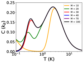
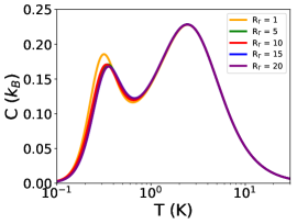
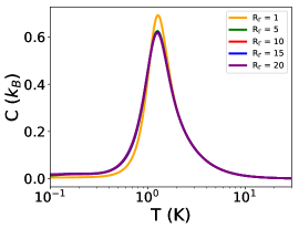
Figure S1: (Color online): Convergence of the heat capacity profiles (per mole of the magnetic ion) on the $32$ site pyrochlore cluster as a function of temperature. The left panel shows results for YbTO for increasing $M$ for fixed $R_{\Gamma}=15$ ($R=120$ total seeds). The center and right panels show results for increasing $R_{\Gamma}$ (for fixed $M=100$) for YbTO and ErTO respectively.

II Details of the numerical calculations

The $32$ site cluster studied in the paper, has $2$ cells in each direction of the FCC primitive lattice vectors. The view of this cluster along the global [111] direction, and the directions in which the periodic boundary conditions are applied have been shown in Fig. 1 of the main text. We have employed its translational symmetries with momentum directions labelled ${\bf{k}}=(k_{1},k_{2},k_{3})$, the former two representing translations perpendicular to the global [111] direction and the latter along [111]. For the $32$ site cluster each $k_{i}=0$ or $k_{i}=\pi$ giving rise to a total of $8$ momentum sectors. The Hilbert space in each momentum sector is approximately $536$ million dimensional. In Fig. 3 and Fig. 5 of the main text, the lowest lying energies are mapped out in all $8$ momentum sectors as a function of parameters in the Hamiltonian (field for Fig. 3 and $\lambda$ for Fig. 5).

Calculations with each starting random vector took roughly $10$ hours on $48$ cores on the MARCC supercomputer for $M=100$ Lanczos iterations. Larger number of iterations were needed ($M=200-400$) for studying low energy spectra. Observables that commute with the Hamiltonian (such as the specific heat) are calculated using the formulae Prelovsek and Bonca (2013),

$$\langle A\rangle = \frac{1}{Z}\sum_{\Gamma}\frac{N_{\Gamma}}{R_{\Gamma}}\sum_{r=1}^{R_{\Gamma}}\sum_{j=1}^{M}\exp(-\beta E_{jr})|\langle r|\psi_{jr}\rangle|^{2}A_{jr}$$ (S7)

$$Z = \sum_{\Gamma}\frac{N_{\Gamma}}{R_{\Gamma}}\sum_{r=1}^{R_{\Gamma}}\sum_{j=1}^{M}\exp(-\beta E_{jr})|\langle r|\psi_{jr}\rangle|^{2}$$ (S8)

where $\beta$ is the inverse temperature, $\Gamma$ is a symmetry (sector) index, $N_{\Gamma}$ is the (sector) Hilbert space size, $|r\rangle$ is a random vector (in the given sector) used to start the Lanczos iteration, $R_{\Gamma}$ is the number of such starting vectors, $\psi_{jr}$ is the $j^{th}$ eigenvector obtained after $M$ iterations (with $|r\rangle$ as the start vector), $E_{jr}$ is the corresponding Ritz eigenenergy and $A_{jr}=\langle\psi_{jr}|A|r\rangle/\langle\psi_{jr}|r\rangle$

In the main text, we also mentioned that the finite temperature Lanczos method (FTLM) works well because only a small number of Krylov space vectors ($M$) and starting vectors ($R_{\Gamma}$ in every symmetry sector) are needed to obtain accurate results. (Note that since there are $8$ symmetry sectors, $R=8R_{\Gamma}$). To validate this claim we show the convergence properties by varying $M$ and fixed $R_{\Gamma}$, and varying $R_{\Gamma}$ at fixed $M$ in Fig. S1.

For example, Fig. S1 shows our results for YbTO when we fix $R_{\Gamma}=15$ and vary $M$. As expected, the high temperature features converged the fastest with increasing $M$, for example, the entire Schottky anomaly centered at $2.4$ K converges by $M=20$. By $M=50$ other lower temperature features have also converged, this is verified by going all the way to $M=100$.

In the central panel, we fix $M=100$ and vary $R_{\Gamma}$. It is remarkable that a single random vector per sector $R_{\Gamma}=1$ is sufficient for reasonably representing the Schottky anomaly. However, to obtain other features quantitatively, one needs $R_{\Gamma}\geq 5$ to converge features on the log scale shown. Finer features associated with the "peak" at $T\approx 0.34$ K show small variations ($0.02$ K) between $R_{\Gamma}=5$ to $R_{\Gamma}=15$ but converge by $R_{\Gamma}=20$. The right panel of the figure shows analogous results for ErTO.

III Comparison of magnetization profiles

In the main text, we showed representative magnetization ($M$) profiles as a function of temperature ($T$) as part of Fig. 4. Here we clarify that quantum effects are crucial for explaining the trends seen in recent experiments in a [111] magnetic field Scheie et al. (2017).

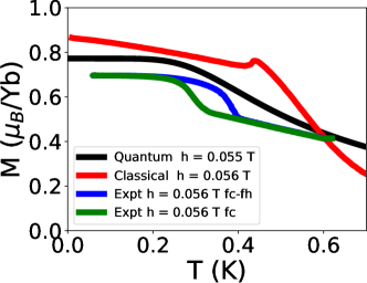
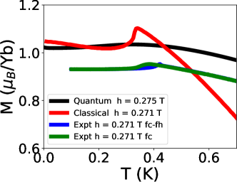
Figure S2: (Color online): Quantum and classical magnetization ($M$), measured along the same direction as the applied [111] magnetic field ($h$) versus temperature ($T$). Comparisons are made to two experimental profiles (with similar field values), left for $h=0.055$ T and right for $h=0.275$ T. fc and fh refer to field cooled and field heated measurements respectively.

Fig. S2 shows our results for two field strengths ($h$). At low temperatures, $M$ vs $T$ is relatively flat, a feature captured quantum mechanically but not classically. Moreover, at $h=0.055$ T the classical kink in the magnetization is at much higher temperature, consistent with a larger $T_{c}$ seen classically. In addition, classically, the change in $M$ with $T$ is more rapid in the paramagnetic regime in comparison to experiments.

In contrast, the quantum calculations largely agree with experiments and correct both these discrepancies. The mild disagreements with experiments are attributed to a combination of finite size effects, inaccurate parameters and presence of magnetic domains in real systems.

References

- Henley (1989) C. L. Henley, Phys. Rev. Lett. 62, 2056 (1989).
- Villain et al. (1980) J. Villain, R. Bidaux, J.-P. Carton, and R. Conte, J. Phys. France 41, 1263 (1980).
- Ross et al. (2011) K. A. Ross, L. Savary, B. D. Gaulin, and L. Balents, Phys. Rev. X 1, 021002 (2011).
- Savary and Balents (2012) L. Savary and L. Balents, Phys. Rev. Lett. 108, 037202 (2012).
- Bloete et al. (1969) H. Bloete, R. Wielinga, and W. Huiskamp, Physica 43, 549 (1969).
- Hermele et al. (2004) M. Hermele, M. P. A. Fisher, and L. Balents, Phys. Rev. B 69, 064404 (2004).
- Bernal and Fowler (1933) J. D. Bernal and R. H. Fowler, The Journal of Chemical Physics 1, 515 (1933).
- Ramirez et al. (1999) A. P. Ramirez, A. Hayashi, R. J. Cava, R. Siddharthan, and B. S. Shastry, Nature 399, 333 (1999).
- Bramwell and Gingras (2001) S. T. Bramwell and M. J. P. Gingras, Science 294, 1495 (2001).
- Pan et al. (2014) L. Pan, S. K. Kim, A. Ghosh, C. M. Morris, K. A. Ross, E. Kermarrec, B. D. Gaulin, S. M. Koohpayeh, O. Tchernyshyov, and N. P. Armitage, Nat. Comm. 5, 4970 (2014).
- Wan and Tchernyshyov (2012) Y. Wan and O. Tchernyshyov, Phys. Rev. Lett. 108, 247210 (2012).
- Applegate et al. (2012) R. Applegate, N. R. Hayre, R. R. P. Singh, T. Lin, A. G. R. Day, and M. J. P. Gingras, Phys. Rev. Lett. 109, 097205 (2012).
- Robert et al. (2015) J. Robert, E. Lhotel, G. Remenyi, S. Sahling, I. Mirebeau, C. Decorse, B. Canals, and S. Petit, Phys. Rev. B 92, 064425 (2015).
- Jaubert et al. (2015) L. D. C. Jaubert, O. Benton, J. G. Rau, J. Oitmaa, R. R. P. Singh, N. Shannon, and M. J. P. Gingras, Phys. Rev. Lett. 115, 267208 (2015).
- Yan et al. (2017) H. Yan, O. Benton, L. Jaubert, and N. Shannon, Phys. Rev. B 95, 094422 (2017).
- Scheie et al. (2017) A. Scheie, J. Kindervater, S. Säubert, C. Duvinage, C. Pfleiderer, H. J. Changlani, S. Zhang, L. Harriger, K. Arpino, S. M. Koohpayeh, O. Tchernyshyov, and C. Broholm, Phys. Rev. Lett. 119, 127201 (2017).
- Chang et al. (2012) L.-J. Chang, S. Onoda, Y. Su, Y.-J. Kao, K.-D. Tsuei, Y. Yasui, K. Kakurai, and M. R. Lees, Nat. Comm. 3, 992 (2012), article.
- Onoda and Tanaka (2011) S. Onoda and Y. Tanaka, Phys. Rev. B 83, 094411 (2011).
- Hayre et al. (2013) N. R. Hayre, K. A. Ross, R. Applegate, T. Lin, R. R. P. Singh, B. D. Gaulin, and M. J. P. Gingras, Phys. Rev. B 87, 184423 (2013).
- Shannon et al. (2012) N. Shannon, O. Sikora, F. Pollmann, K. Penc, and P. Fulde, Phys. Rev. Lett. 108, 067204 (2012).
- Kato and Onoda (2015) Y. Kato and S. Onoda, Phys. Rev. Lett. 115, 077202 (2015).
- Jaklic and Prelovsek (1994) J. Jaklic and P. Prelovsek, Phys. Rev. B 49, 5065 (1994).
- Prelovsek and Bonca (2013) P. Prelovsek and J. Bonca, “Ground state and finite temperature lanczos methods,” in Strongly Correlated Systems: Numerical Methods, edited by A. Avella and F. Mancini (Springer Berlin Heidelberg, Berlin, Heidelberg, 2013) pp. 1–30.
- Thompson et al. (2017) J. D. Thompson, P. A. McClarty, D. Prabhakaran, I. Cabrera, T. Guidi, and R. Coldea, Phys. Rev. Lett. 119, 057203 (2017).
- Arpino et al. (2017) K. E. Arpino, B. A. Trump, A. O. Scheie, T. M. McQueen, and S. M. Koohpayeh, Phys. Rev. B 95, 094407 (2017).
- Pe çanha Antonio et al. (2017) V. Pe çanha Antonio, E. Feng, Y. Su, V. Pomjakushin, F. Demmel, L.-J. Chang, R. J. Aldus, Y. Xiao, M. R. Lees, and T. Brückel, Phys. Rev. B 96, 214415 (2017).
- Savary et al. (2012) L. Savary, K. A. Ross, B. D. Gaulin, J. P. C. Ruff, and L. Balents, Phys. Rev. Lett. 109, 167201 (2012).
- Dalmas de Réotier et al. (2012) P. Dalmas de Réotier, A. Yaouanc, Y. Chapuis, S. H. Curnoe, B. Grenier, E. Ressouche, C. Marin, J. Lago, C. Baines, and S. R. Giblin, Phys. Rev. B 86, 104424 (2012).
- Niven et al. (2014) J. F. Niven, M. B. Johnson, A. Bourque, P. J. Murray, D. D. James, H. A. Dabkowska, B. D. Gaulin, and M. A. White, Proceedings of the Royal Society of London A: Mathematical, Physical and Engineering Sciences 470 (2014), 10.1098/rspa.2014.0387.
- Curnoe (2007) S. H. Curnoe, Phys. Rev. B 75, 212404 (2007).
- Onoda (2011) S. Onoda, Journal of Physics: Conference Series 320, 012065 (2011).
- Hanebaum and Schnack (2014) O. Hanebaum and J. Schnack, The European Physical Journal B 87, 194 (2014).
- Oitmaa et al. (2013) J. Oitmaa, R. R. P. Singh, B. Javanparast, A. G. R. Day, B. V. Bagheri, and M. J. P. Gingras, Phys. Rev. B 88, 220404 (2013).
- Zhitomirsky et al. (2012) M. E. Zhitomirsky, M. V. Gvozdikova, P. C. W. Holdsworth, and R. Moessner, Phys. Rev. Lett. 109, 077204 (2012).
- Hallas et al. (2017) A. M. Hallas, J. Gaudet, and B. D. Gaulin, ArXiv e-prints (2017), arXiv:1708.01312 [cond-mat.str-el] .
- Kumar et al. (2016) K. Kumar, H. J. Changlani, B. K. Clark, and E. Fradkin, Phys. Rev. B 94, 134410 (2016).
- Yasui et al. (2003) Y. Yasui, M. Soda, S. Iikubo, M. Ito, M. Sato, N. Hamaguchi, T. Matsushita, N. Wada, T. Takeuchi, N. Aso, and K. Kakurai, Journal of the Physical Society of Japan 72, 3014 (2003).
- Bruognolo et al. (2017) B. Bruognolo, Z. Zhu, S. R. White, and E. Miles Stoudenmire, ArXiv e-prints (2017), arXiv:1705.05578 [cond-mat.str-el] .
- Claes and Clark (2017) J. Claes and B. K. Clark, Phys. Rev. B 95, 205109 (2017).
- Changlani et al. (2009) H. J. Changlani, J. M. Kinder, C. J. Umrigar, and G. K.-L. Chan, Phys. Rev. B 80, 245116 (2009).
- Holmes et al. (2016a) A. A. Holmes, H. J. Changlani, and C. J. Umrigar, Journal of Chemical Theory and Computation 12, 1561 (2016a).
- Petruzielo et al. (2012) F. R. Petruzielo, A. A. Holmes, H. J. Changlani, M. P. Nightingale, and C. J. Umrigar, Phys. Rev. Lett. 109, 230201 (2012).
- Holmes et al. (2016b) A. A. Holmes, N. M. Tubman, and C. J. Umrigar, Journal of Chemical Theory and Computation 12, 3674 (2016b).
- Tubman et al. (2016) N. M. Tubman, J. Lee, T. Y. Takeshita, M. Head-Gordon, and K. B. Whaley, The Journal of Chemical Physics 145, 044112 (2016).
- Blunt et al. (2015) N. S. Blunt, A. Alavi, and G. H. Booth, Phys. Rev. Lett. 115, 050603 (2015).