Entropic relations for retrodicted quantum measurements

Abstract

Given an arbitrary measurement over a system of interest, the outcome of a posterior measurement can be used for improving the statistical estimation of the system state after the former measurement. Here, we realize an informational-entropic study of this kind of (Bayesian) retrodicted quantum measurement formulated in the context of quantum state smoothing. We show that the (average) entropy of the system state after the retrodicted measurement (smoothed state) is bounded from below and above by the entropies of the first measurement when performed in a selective and non-selective standard predictive ways respectively. For bipartite systems the same property is also valid for each subsystem. Their mutual information, in the case of a former single projective measurement, is also bounded in a similar way. The corresponding inequalities provide a kind of retrodicted extension of Holevo bound for quantum communication channels. These results quantify how much information gain is obtained through retrodicted quantum measurements in quantum state smoothing. While an entropic reduction is always granted, in bipartite systems mutual information may be degraded. Relevant physical examples confirm these features.

I Introduction

Prediction and retrodiction are different and alternative ways of handling information. Respectively, information in the past or in the future is taken into account for performing a probabilistic (Bayesian) statement about a system of interest. In physics, most of the theoretical frames are formulated in a predictive way. The measurement process in quantum mechanics is clearly predictive. The corresponding information changes are well known. Non-selective projective measurements never decrease von Neumann entropy nielsen . Furthermore, the entropy $\mathcal{S}[\rho]\equiv-\mathrm{Tr}[\rho\ln\rho]$ after a measurement performed in a non-selective way is always greater than the (average) entropy of the same measurement performed in a selective way breuerbook , that is, $\mathcal{S}[\sum_{k}p(k)\rho_{k}]\geq\sum_{k}p(k)\mathcal{S}[\rho_{k}],$ where $\rho_{k}$ and $p(k)$ are respectively the system state and probability associated to each outcome $k.$ Their difference is bounded by Shannon entropy $\mathcal{H}[k]\equiv-\sum_{k}p(k)\ln[p(k)]$ of the outcomes probabilities $\{p(k)\},$ $\mathcal{H}[k]\geq\mathcal{S}[\sum_{k}p(k)\rho_{k}]-\sum_{k}p(k)\mathcal{S}[\rho_{k}].$ These statements follows straightforwardly from Klein inequality and the concavity of von Neumann entropy nielsen ; breuerbook . Much less is known when the quantum measurement process is performed in a retrodictive way.

In quantum mechanics, retrodiction was introduced for criticizing the apparent time asymmetry of the measurement process aharonov ; vaidman . Pre- and post-selected measurement ensembles (initial and final states are known) are considered. Questions about intermediate states are characterized through a (retrodictive) Bayesian analysis and the standard Born rule.

Retrodiction also arises in the related formalisms of past quantum states molmer and quantum state smoothing wiseman ; tsang , which can be considered as a quantum extension of classical (Bayesian inference) smoothing techniques jaz ; recipes . Both information in the past and in the future of an open quantum system continuously monitored in time milburn ; carmichaelbook is available. Hence, the system information is described through a pair of operators, the past quantum state, consisting in the system density matrix and an effect operator that takes into account the future information molmer . These objects allow to estimate the outcome probabilities of an intermediate (retrodicted) quantum measurement process taking into account both past and future information. The previous scheme was studied and applied in a wide class of dynamics and physical arrangements tsanPRA ; meschede ; murch ; haroche ; xu ; tan ; naghi ; huard ; decay . The system state (single density matrix) that takes into account both past and future information is called quantum smoothed state wiseman ; retro .

While in general it is argued that extra (future) information improves the estimation of a past (retrodicted) measurement, in contrast with predictive measurements, a rigorous quantification of this informational benefit is lacking. Hence, the goal of this paper is to perform an informational-entropic study of retrodictive quantum measurements. We find upper and lower bounds for the (average) entropy of the retrodicted state (quantum smoothed state). They are defined by the entropies of the same measurement without retrodiction and performed in a non-selective and selective ways respectively. The same kind of relation is obtained for each part of a bipartite system. Their mutual information satisfies similar inequalities whose explicit form (in the case of projective retrodictive measurements) leads to a kind of retrodicted extension of Holevo bound for quantum communication channels nielsen . These features are exemplified with a qubit submitted to strong-weak retrodicted measurements murch and a hybrid quantum-classical optical-like arrange molmer .

The developed results provide a rigorous characterization of the information changes achieved through retrodicted quantum measurements. The analysis is performed in the context of past quantum states and quantum state smoothing molmer ; wiseman ; tsang . We remark that retrodicted measurements were also introduced in alternative ways barnett ; pegg . Some similitudes and differences become clear through the present study.

The paper is outlined as follows. In Sec. II we present the general structure of retrodicted measurements and quantum state smoothing. In Sec. III the general entropic relations are obtained. The case of bipartite system is also characterized through their mutual information. In Sec. IV we study the case of projective measurement performed over a subsystem of a bipartite arrangement. Retrodicted-like Holevo bounds are derived. Examples are worked out in Sec. V. In Sec. VI we provide the Conclusions. Calculus details that support the main results are presented in the Appendices.

II Retrodicted quantum measurements

Here we present the basic scheme (see Fig. 1) corresponding to a retrodicted quantum measurement. It recovers the past quantum state formalism molmer and also allows us to define a quantum smoothed state wiseman ; retro .

A quantum system is characterized by its density matrix $\rho_{I}.$ This object depends on the previous history of the system. In a first step, it is subjected to an arbitrary measurement process nielsen ; breuerbook defined by the set of measurement operators $\{\Omega_{m}\},$ which fulfills $\sum\nolimits_{m}\Omega_{m}^{\dagger}\Omega_{m}=\mathrm{I,}$ where $\mathrm{I}$ is the identity matrix in the system Hilbert space. The system states $\{\rho_{m}\}$ associated to each outcome, and the probability $\{p(m)\}$ of their occurrence, respectively are

$$\rho_{m}=\frac{\Omega_{m}\rho_{I}\Omega_{m}^{\dagger}}{\mathrm{Tr}[\Omega_{m}^{\dagger}\Omega_{m}\rho_{I}]},\ \ \ \ \ p(m)=\mathrm{Tr}[\Omega_{m}^{\dagger}\Omega_{m}\rho_{I}],$$ (1)

where $\mathrm{Tr}[\bullet]$ is the trace operation.

After the first measurement, the system evolves with its own (reversible or irreversible) completely positive dynamics nielsen ; breuerbook and then is subjected to a second arbitrary measurement process. It is defined by a set of operators $\{M_{y}\},$ which satisfy $\sum\nolimits_{y}M_{y}^{\dagger}M_{y}=\mathrm{I.}$ In the following analysis the system dynamics is disregarded, or equivalently, it can be taken into account through a redefinition of the set of operators $\{M_{y}\}.$

The second measurement implies the state transformation $\rho_{m}\rightarrow M_{y}\rho_{m}M_{y}^{\dagger}/\mathrm{Tr}[M_{y}^{\dagger}M_{y}\rho_{m}].$ The (conditional) probability $p(y|m)$ of outcome $y$ given that the first one was $m$ reads

$$p(y|m)=\mathrm{Tr}[M_{y}^{\dagger}M_{y}\rho_{m}]=\frac{\mathrm{Tr}[\Omega_{m}\rho_{I}\Omega_{m}^{\dagger}M_{y}^{\dagger}M_{y}]}{\mathrm{Tr}[\Omega_{m}^{\dagger}\Omega_{m}\rho_{I}]}.$$ (2)

An essential ingredient for defining a retrodicted measurement is to ask about the inverse conditional probability $p(m|y),$ that is, the probability of $m$ given the (posterior) outcome $y.$ This object follows from Bayes rule. Given that the joint probability $p(y,m)$ for the measurement events $m$ and $y$ satisfies $p(y,m)=p(y|m)p(m),$ it reads

$$p(y,m)=\mathrm{Tr}[\Omega_{m}\rho_{I}\Omega_{m}^{\dagger}M_{y}^{\dagger}M_{y}].$$ (3)

Now, by using that $p(y,m)=p(m|y)p(y),$ where

$$p(y)=\sum_{m}p(m,y),$$ (4)

is the probability of outcome $y,$ we obtain

$$p(m|y)=\frac{\mathrm{Tr}[\Omega_{m}\rho_{I}\Omega_{m}^{\dagger}M_{y}^{\dagger}M_{y}]}{\sum_{m^{\prime}}\mathrm{Tr}[\Omega_{m^{\prime}}\rho_{I}\Omega_{m^{\prime}}^{\dagger}M_{y}^{\dagger}M_{y}]}.$$ (5)

This retrodicted probability relies on Bayes rules and standard quantum measurement theory. It arises in pre- and post-selected ensembles (here defined by $\rho_{I}$ and the outcome $y)$ aharonov ; vaidman and also in the past quantum state formalism (see supplemental material in Ref. molmer ). In fact, $p(m|y)$ can be written in terms of the past quantum state $\Xi\equiv(\rho,E)$ where the density and effect operators are $\rho=\rho_{I}$ and $E=M_{y}^{\dagger}M_{y}$ respectively.

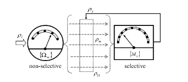
Figure 1: Scheme of retrodicted measurements. The system is subjected to two successive measurement processes defined by the operators $\{\Omega_{m}\}$ and $\{M_{y}\}$ respectively. From the second outcome one infers the probability for the first outcome. The system state at the different stages is explained in the text.

Retrodicted-Quantum smoothed state

The previous analysis does not associate or define a system state to the retrodicted probability $p(m|y).$ This assignation depends on extra assumptions. Similarly to Ref. molmer we assume that the result of the first measurement is hidden to us, that is, the first measurement is a non-selective one nielsen ; breuerbook . Hence, the system state after the first measurement, $\rho_{I}\rightarrow\rho_{\Omega},$ is

$$\rho_{\Omega}=\sum_{m}\rho_{m}\ p(m)=\sum_{m}\Omega_{m}\rho_{I}\Omega_{m}^{\dagger}.$$ (6)

The retrodicted or smoothed quantum state $\rho_{y}$ wiseman ; retro here is defined as the estimation of the system state after the first non-selective measurement given that we know the outcome (labeled by $y$) of the second (selective) measurement. Therefore, we write

$$\rho_{y}\equiv\sum_{m}\rho_{m}\ p(m|y)=\sum_{m}w(m,y)\Omega_{m}\rho_{I}\Omega_{m}^{\dagger}.$$ (7)

Here, $w(m,y)\equiv p(m|y)/p(m)=p(y,m)/[p(y)p(m)],$ which from Eqs. (1) and (5) explicitly reads

$$w(m,y)=\frac{\mathrm{Tr}[\Omega_{m}\rho_{I}\Omega_{m}^{\dagger}M_{y}^{\dagger}M_{y}]}{\mathrm{Tr}[\Omega_{m}^{\dagger}\Omega_{m}\rho_{I}]\sum_{m^{\prime}}\mathrm{Tr}[\Omega_{m^{\prime}}\rho_{I}\Omega_{m^{\prime}}^{\dagger}M_{y}^{\dagger}M_{y}]}.$$ (8)

We remark that the smoothed state $\rho_{y}$ depends of (is conditioned to) the result of the second measurement. Contrarily to the case of pre- and post selected measurements aharonov ; vaidman , where $y$ is fixed, here not any selection is imposed on the second measurement result. Therefore, we can define an average smoothed state $\rho_{M}\equiv\sum_{y}\rho_{y}\ p(y),$ which corresponds to the system state after averaging $\rho_{y}$ over the outcomes $y.$ Using that $p(y)=\sum_{m^{\prime}}\mathrm{Tr}[\Omega_{m^{\prime}}\rho_{I}\Omega_{m^{\prime}}^{\dagger}M_{y}^{\dagger}M_{y}]$ [see Eq. (3)] and that $\sum_{y}M_{y}^{\dagger}M_{y}=\mathrm{I},$ it follows

$$\rho_{M}\equiv\sum_{y}\rho_{y}\ p(y)=\sum_{m}\rho_{m}\ p(m)=\rho_{\Omega}.$$ (9)

Thus, the average smoothed state $\rho_{M}$ recovers the state $\rho_{\Omega}$ corresponding to the state after the first non-selective measurement. A similar property was found in the quantum-classical arrangements studied in Ref. retro .

The analysis of retrodicted quantum measurements performed in Refs. barnett ; pegg also rely on quantum measurement theory and Bayes rule. Nevertheless, the assumptions are different to the previous ones. After the second measurement, the state $\rho_{m}$ are not known. Hence, the state after the first measurement [Eq. (6)] is taken as a state of maximal entropy, $\rho_{\Omega}\simeq\mathrm{I,}$ while $\rho_{y}$ [Eq. (7)] looses its meaning. Hence, the following results do not apply straightforwardly to those models.

III Entropic relations

The retrodicted quantum measurement scheme described previously consists in two, non-selective and selective, successive measurements. Now, the relevant question is how much information gain is obtained from the retrodicted (smoothed) state $\rho_{y}$ [Eq.(7)]. As usual, as an information measure we consider the von Neumann entropy $\mathcal{S}[\rho]=-\mathrm{Tr}[\rho\ln\rho].$ In general, one is interested in establishing upper and lower bounds for $\mathcal{S}[\rho_{y}],$ and to determine how they are related with, for example, the entropies $\mathcal{S}[\rho_{\Omega}]$ or $\mathcal{S}[\rho_{m}].$

Given the arbitrariness of the two measurement processes and given the random nature of the outcome $y,$ it is not possible to establishing any general relation between the entropies $\mathcal{S}[\rho_{y}],$ $\mathcal{S}[\rho_{\Omega}],$ and $\mathcal{S}[\rho_{m}].$ Any relation is in fact possible. Therefore, similarly to the case of standard measurement process nielsen ; breuerbook , any entropy relation must be established by considering averages over the possible measurement outcomes.

By using the concavity of the von Neumann entropy, $\mathcal{S}[\sum_{k}p(k)\rho_{k}]\geq\sum_{k}p(k)\mathcal{S}[\rho_{k}]$ nielsen (with equality if and only if all states $\rho_{k}$ are the same), in Appendix A we derive the following entropy relation

$$\mathcal{S}[\rho_{\Omega}]\geq\sum_{y}p(y)\mathcal{S}[\rho_{y}]\geq\sum_{m}p(m)\mathcal{S}[\rho_{m}].$$ (10)

This is one of the central results of this paper. It demonstrates that the (average) entropy of the system after the retrodicted measurement, $\sum_{y}p(y)\mathcal{S}[\rho_{y}],$ is bounded from above and below by the entropies of its associated non-selective, $\mathcal{S}[\rho_{\Omega}],$ and (average) selective, $\sum_{m}p(m)\mathcal{S}[\rho_{m}],$ measurement entropies. In other words, the retrodictive measurement is more informative than the first non-selective measurement, but is less informative than a selective resolution of the same measurement process.

In Eq. (10), the lower bound is achieved when all states $\{\rho_{m}\}$ are the same, or alternatively when $p(m|y)=\delta_{my},$ that is, both measurement result are completely correlated, $p(y,m)=\delta_{ym}p(m)=\delta_{my}p(y)$ in Eq. (3). On the other hand, the upper bound is fulfilled when all states $\{\rho_{y}\}$ are the same. This last condition occurs when all states $\{\rho_{m}\}$ are identical, or alternatively when $p(m|y)=p(m).$ Hence, both measurement results, $\{m\}$ and $\{y\},$ are statistically independent, $p(y,m)=p(y)p(m)$ in Eq. (3) (see Appendix A).

Interestingly, it is also possible to bound the difference between the terms appearing in Eq. (10). By using the upper bound $\sum_{k}p(k)\mathcal{S}[\rho_{k}]+\mathcal{H}[k]\geq\mathcal{S}[\sum_{k}p(k)\rho_{k}]$ nielsen , where $\mathcal{H}[k]=-\sum_{k}p(k)\ln[p(k)]$ is the Shannon entropy of a probability distribution $\{p(k)\},$ in Appendix A we obtain

$$\mathcal{H}[y]\geq\mathcal{S}[\rho_{\Omega}]-\sum_{y}p(y)\mathcal{S}[\rho_{y}]\geq 0,$$ (11)

while in the other extreme it is valid that

$$\mathcal{H}[m]\geq\sum_{y}p(y)\mathcal{S}[\rho_{y}]-\sum_{m}p(m)\mathcal{S}[\rho_{m}]\geq 0.$$ (12)

In this way, the Shannon entropies $\mathcal{H}[y]$ and $\mathcal{H}[m]$ (associated to the two measurement outcomes) bound the difference between the entropies of the retrodicted and its associated non-selective and selective measurements. Conditions under which the upper bounds of Eqs. (11) and (12) are achieved are also provided in Appendix A.

III.1 Bipartite systems

In many physical arrangements where the retrodicted measurement scheme was studied, the system of interest is a bipartite one. Thus, a relevant question is to determine if the previous entropy inequality [Eq. (10)] remains valid (or not) for each subsystem.

Denoting by $A$ and $B$ each subsystem, their states follow from the partial traces $\rho^{a}=\mathrm{Tr}_{b}[\rho^{ab}],$ and $\rho^{b}=\mathrm{Tr}_{a}[\rho^{ab}],$ where $\rho^{ab}$ is an arbitrary bipartite state. Under the replacements $\rho_{m}\rightarrow\rho_{m}^{a/b},$ $\rho_{y}\rightarrow\rho_{y}^{a/b},$ $\rho_{\Omega}\rightarrow\rho_{\Omega}^{a/b},$ from the demonstrations of Appendix A it is simple to realize that the inequalities Eqs. (10), (11), and (12) remain valid for each subsystem. This result is valid independently of which kind of (bipartite) measurements are performed.

III.2 Mutual information

Another important aspect that can be studied when considering bipartite systems is the change in the mutual information between the subsystems. For a bipartite state $\rho^{ab},$ the mutual information $\mathcal{I}[\rho^{ab}]$ is defined as $\mathcal{I}[\rho^{ab}]\equiv\mathcal{S}[\rho^{a}]+\mathcal{S}[\rho^{b}]-\mathcal{S}[\rho^{ab}].$ As demonstrated in Appendix B, bounds for this object can be derived by using the strong subadditivity property of von Neumann entropy, $\mathcal{S}[\rho_{abc}]+\mathcal{S}[\rho_{a}]\leq\mathcal{S}[\rho_{ab}]+\mathcal{S}[\rho_{ac}].$ Thus, as usual in quantum information results nielsen , the demonstrations rely on introducing an extra ancilla system.

In Appendix B we demonstrate that

$$\mathcal{S}[\rho_{\Omega}^{ab}]-\sum_{y}p(y)\mathcal{S}[\rho_{y}^{ab}]\geq\mathcal{I}[\rho_{\Omega}^{ab}]-\sum_{y}p(y)\mathcal{I}[\rho_{y}^{ab}].$$ (13)

Therefore, the difference between the mutual information corresponding to the non-selective measurement, $\mathcal{I}[\rho_{\Omega}^{ab}],$ and the average mutual information corresponding to the retrodicted one, $\sum_{y}p(y)\mathcal{I}[\rho_{y}^{ab}],$ is bounded by the positive quantity $\mathcal{S}[\rho_{\Omega}^{ab}]-\sum_{y}p(y)\mathcal{S}[\rho_{y}^{ab}]$ [see Eq. (11)]. On the other hand, based on the strong subadditivity condition, it is also possible to show that

$$\sum_{y}p(y)\mathcal{S}[\rho_{y}^{ab}]-\sum_{m}p(m)\mathcal{S}[\rho_{m}^{ab}]\geq$$

$$\sum_{y}p(y)\mathcal{I}[\rho_{y}^{ab}]-\sum_{m}p(m)\mathcal{I}[\rho_{m}^{ab}].$$ (14)

This inequality, which is similar to the previous one, here gives an upper bound for the difference between the (average) mutual information corresponding to the retrodicted measurement, $\sum_{y}p(y)\mathcal{I}[\rho_{y}^{ab}],$ and its (non-retrodicted) selective resolution, $\sum_{m}p(m)\mathcal{I}[\rho_{m}^{ab}].$ From Eq. (12) it follows that the upper bound $\sum_{y}p(y)\mathcal{S}[\rho_{y}^{ab}]-\sum_{m}p(m)\mathcal{S}[\rho_{m}^{ab}]$ is a positive quantity.

General conditions under which the previous bounds [Eqs. (13) and (14)] become equalities are left open equality . On the other hand, notice that only upper bounds were found.

IV Projective measurements in bipartite systems

The previous results are general and apply independently of the nature of the measurement processes (Fig. 1). Here, we consider an arbitrary bipartite system where a first projective measurement is performed on subsystem $B,$ while the posterior one remains arbitrary being performed over subsystem $A.$ Hence, the operators $\{\Omega_{m}\}$ that define the first measurement are written as

$$\Omega_{m}=\mathrm{I}_{a}\otimes|m\rangle\langle m|.$$ (15)

Here, $\mathrm{I}_{a}$ is the identity matrix in the Hilbert space of subsystem $A$ while $\{|m\rangle\}$ is a complete orthogonal base of $B.$ The second measurement is defined by the set of operators $\{M_{y}\},$ which act on the Hilbert space of $A.$

The bipartite state associated to each outcome $\{m\}$ reads [Eq. (1)]

$$\rho_{m}^{ab}=\frac{\langle m|\rho_{I}|m\rangle}{\mathrm{Tr}_{a}[\langle m|\rho_{I}|m\rangle]}\otimes|m\rangle\langle m|\equiv\rho_{m}^{a}\otimes|m\rangle\langle m|.$$ (16)

The state after the non-selective measurements is [Eq. (6)]

$$\rho_{\Omega}^{ab}=\sum_{m}p(m)\rho_{m}^{a}\otimes|m\rangle\langle m|,$$ (17)

while the retrodictive smoothed state becomes [Eq. (7)]

$$\rho_{y}^{ab}=\sum_{m}p(m|y)\rho_{m}^{a}\otimes|m\rangle\langle m|.$$ (18)

From Eqs. (16) to (18) it is possible to demonstrate (Appendix C) that in fact the inequalities (10) and bounds defined by Eqs. (11) and (12) are explicitly satisfied by the bipartite states. Similar expressions are valid for each subsystem.

IV.1 Mutual information

The changes in the mutual information at the different measurement stages are upper bounded by Eqs. (13) and (14). Given the projective character of the first measurement, here it is also possible to find a lower bound to these informational changes.

From Eqs. (13) and Eqs. (16) to (18), in Appendix C we obtain

$$\mathcal{H}\left[m:y\right] \geq \mathcal{I}[\rho_{\Omega}^{ab}]-\sum_{y}p(y)\mathcal{I}[\rho_{y}^{ab}]$$ (19a)

$$= \mathcal{S}[\rho_{\Omega}^{a}]-\sum_{y}p(y)\mathcal{S}[\rho_{y}^{a}]\geq 0.$$ (19b)

where $$\mathcal{H}[m:y]=\mathcal{H}[m]+\mathcal{H}[y]-\mathcal{H}[m,y], \{m\} \{y\}. \sum_{y}p(y)\mathcal{I}[\rho_{y}^{ab}], \mathcal{I}[\rho_{\Omega}^{ab}].$$ is the classical mutual information between the outcomes of both measurements, and The lower bound in the previous expression say us that the (average) mutual information associated to the retrodicted measurement, is smaller than that corresponding to the non-selective measurement, Hence, contrarily to the entropy measure, here the retrodicted measurement leads to a degradation of the mutual information between the subsystems. Similarly to Eq. (19), it is possible to obtain (Appendix C)

$$\mathcal{H}[m|y] \geq \sum_{y}p(y)\mathcal{I}[\rho_{y}^{ab}]-\sum_{m}p(m)\mathcal{I}[\rho_{m}^{ab}]$$ (20a)

$$= \sum_{y}p(y)\mathcal{S}[\rho_{y}^{a}]-\sum_{m}p(m)\mathcal{S}[\rho_{m}^{a}]\geq 0,\ \ \ \ \ \ \$$ (20b)

where, as before, $$\mathcal{H}[m|y] \{m\} \{y\}. \sum_{m}p(m)\mathcal{I}[\rho_{m}^{ab}].$$ is the conditional entropy of outcomes given outcomes Thus, while the mutual information associated to the retrodictive measurement decreases with respect to the non-selective measurement, it is bounded from below by the mutual information of its selective resolution,

IV.2 Retrodicted-like Holevo bound

Interestingly, Eqs. (19) and (20) can be read as a retrodicted version of the well known Holevo bound for quantum communication channels nielsen .

The standard Holevo bound arises in the following context. A sender prepare a quantum alphabet $\{\rho_{m}^{a}\}$ with probabilities $\{p(m)\}.$ A receiver performs a measurement characterized by the operators $\{M_{y}\}$ on the sent letter (state), which gives the result $y.$ The Holevo bound states that for any measurement the receiver may do it is fulfilled that nielsen

$$\mathcal{H}[m:y]\leq\mathcal{S}\left[\sum\nolimits_{m}p(m)\rho_{m}^{a}\right]-\sum\nolimits_{m}p(m)\mathcal{S}[\rho_{m}^{a}].$$ (21)

Hence, the accessible channel information (measured by the mutual information $\mathcal{H}[m:y]$ between the preparation and the measurement outcomes), is upper bounded by $\chi\equiv\mathcal{S}\left[\sum\nolimits_{m}p(m)\rho_{m}^{a}\right]-\sum\nolimits_{m}p(m)\mathcal{S}[\rho_{m}^{a}].$

In the retrodicted measurement scheme (Fig. 1), the preparation $\{\rho_{m}^{a}\}$ with probabilities $\{p(m)\}$ can be associated with the first non-selective measurement, while the receiver measurement corresponds to the second one. With this interpretation at hand, we notice that Eq. (19) rewritten as

$$\mathcal{H}\left[m:y\right]\geq\mathcal{S}\left[\sum\nolimits_{y}p(y)\rho_{y}^{a}\right]-\sum_{y}p(y)\mathcal{S}[\rho_{y}^{a}],$$ (22)

can be read as a retrodicted-like Holevo bound. While Holevo bound (21) gives an upper bound for the accessible information, the retrodicted bound [Eq. (19)] gives a lower bound for $\mathcal{H}[m:y].$ Interestingly, it is written in terms of the (retrodicted) quantum smoothed states $\{\rho_{y}^{a}\}.$ A complementary expression follows straightforwardly from Eq. (20).

V Examples

Different experimental realizations of the retrodicted scheme of Fig. 1 are performed with open quantum systems continuously monitored in time. Hence, their description rely on the formalism of stochastic wave vectors milburn ; carmichaelbook . The results developed in the previous sections can be extended to this context. Nevertheless, for simplicity, we consider examples where only two measurements are performed (Fig. 1). The chosen measurement operators capture the main features of different experimental realizations murch ; molmer .

V.1 Weak and strong retrodicted measurements of a qubit

First, we consider a qubit system (two-level system) that starts in an arbitrary state $\rho_{I},$ which is written as

$$\rho_{I}=\frac{1}{2}(\mathrm{I}+\mathbf{r}_{I}\cdot\mathbf{\sigma}).$$ (23)

Here, $\mathrm{I}$ is the identity matrix while $\mathbf{\sigma}=(\sigma_{x},\sigma_{y},\sigma_{z})$ is defined by Pauli matrixes. The Bloch vector nielsen ; breuerbook is defined as $\mathbf{r}_{I}=r_{I}\mathbf{n},$ where its modulus satisfies $0\leq r_{I}=|\mathbf{r}_{I}|\leq 1$ and $\mathbf{n}=(n_{x},n_{y},n_{z})=(\sin(\theta_{I})\cos(\phi_{I}),\sin(\theta_{I})\sin(\phi_{I}),\cos(\theta_{I})).$ Thus, $\rho_{I}=\rho_{I}(r_{I},\theta_{I},\phi_{I}).$

Similarly to Ref. murch , the first measurement operator is given by $(m\rightarrow V)$

$$\Omega_{V}=(2\pi a^{2})^{-1/4}\exp\left[-\frac{(V-\sigma_{z})^{2}}{4a^{2}}\right],$$ (24)

where $a>0$ is a real free parameter and $V\in(-\infty,+\infty),$ which defines the outcomes of the first measurement. Consistently, $\int_{-\infty}^{+\infty}dV\Omega_{V}^{{\dagger}}\Omega_{V}=\mathrm{I.}$ In the experiment analyzed in murch , the second measurement can be related with an effect operator that takes into account the future stochastic evolution. Instead, here we consider an arbitrary qubit projective measurement $(y=\pm)$ performed in an arbitrary direction, which is defined by the angles $(\theta,\phi).$ Hence,

$$M_{\pm}=|n_{\pm}\rangle\langle n_{\pm}|,$$ (25)

$[M_{\pm}=M_{\pm}(\theta,\phi)]$ where the state vectors $|n_{\pm}\rangle$ are

$$|n_{+}\rangle = \cos\Big{(}\frac{\theta}{2}\Big{)}|+\rangle+\sin\Big{(}\frac{\theta}{2}\Big{)}e^{-i\phi}|-\rangle,$$ (26a)

$$|n_{-}\rangle = -\sin\Big{(}\frac{\theta}{2}\Big{)}|+\rangle+\cos\Big{(}\frac{\theta}{2}\Big{)}e^{+i\phi}|-\rangle.$$ (26b)

Here, $$|\pm\rangle \sigma_{z}.$$ are the eigenstates of

The previous definitions completely set the retrodicted measurement scheme of Fig. 1. It depends on the free parameters $(r_{I},\theta_{I},\phi_{I},a,\theta,\phi).$ Our results guarantee that the inequality (10) is fulfilled independently of their values.

The states associated to a selective resolution of the first measurement, $\rho_{V}=\Omega_{V}\rho_{I}\Omega_{V}^{\dagger}/\mathrm{Tr}[\Omega_{V}^{\dagger}\Omega_{V}\rho_{I}]$ [Eq. (1)], can be calculated in an exact way from the following expression

$$\tilde{\rho}_{V}=\sqrt{\frac{1}{2\pi a^{2}}}\left(\begin{array}[]{cc}\langle+|\rho_{I}|+\rangle e^{-\frac{(V-1)^{2}}{2a^{2}}}&\langle+|\rho_{I}|-\rangle e^{-\frac{(V^{2}+1)}{2a^{2}}}\\ \langle-|\rho_{I}|+\rangle e^{-\frac{(V^{2}+1)}{2a^{2}}}&\langle+|\rho_{I}|+\rangle e^{-\frac{(V+1)^{2}}{2a^{2}}}\end{array}\right),$$ (27)

where $\tilde{\rho}_{V}\equiv\Omega_{V}\rho_{I}\Omega_{V}^{\dagger}.$ From this result it is possible to demonstrate that

$$\lim_{a\rightarrow 0}\rho_{V}=|\pm\rangle\langle\pm|,\ \ \ (V\gtrless 0),\ \ \ \ \ \ \ \lim_{a\rightarrow\infty}\rho_{V}=\rho_{I}.$$ (28)

Thus, in the limit $a\rightarrow 0,$ the operators $\{\Omega_{V}\}$ perform a strong projective measurement in the base of eigenstates of $\sigma_{z}.$ On the other hand, in the limit $a\rightarrow\infty,$ a weak measurement weak is performed, $\rho_{V}=\rho_{I}.$

From Eq. (27), after a straightforward calculation, the state $\rho_{\Omega}=\int_{-\infty}^{\infty}dV\ \Omega_{V}\rho_{I}\Omega_{V}^{\dagger}$ [Eq. (6)] can be written as

$$\rho_{\Omega}=\left(\begin{array}[]{cc}\langle+|\rho_{I}|+\rangle&\langle+|\rho_{I}|-\rangle e^{-\frac{1}{2a^{2}}}\\ \langle-|\rho_{I}|+\rangle e^{-\frac{1}{2a^{2}}}&\langle+|\rho_{I}|+\rangle\end{array}\right).$$ (29)

This expression also reflects the strong and weak feature of the (here non-selective) measurement as a function of the parameter $a.$ In fact, when $a\rightarrow 0$ a diagonal matrix follows, while $\lim_{a\rightarrow\infty}\rho_{\Omega}=\rho_{I}.$

From Eq. (27) it is also simple to obtain the probability density $p(V)=\mathrm{Tr}[\Omega_{V}^{\dagger}\Omega_{V}\rho_{I}]=\mathrm{Tr}[\tilde{\rho}_{V}]$ [Eq. (1)], which is defined by a superposition of two shifted Gaussian distributions weighted by the initial populations $\langle\pm|\rho_{I}|\pm\rangle.$ In general, the joint probability $p(\pm,V)=\mathrm{Tr}[\Omega_{V}\rho_{I}\Omega_{V}^{\dagger}M_{\pm}^{\dagger}M_{\pm}]$ [Eq. (3)] reads

$$p(\pm,V) = +\sqrt{\frac{1}{2\pi a^{2}}}e^{-\frac{(V\mp 1)^{2}}{2a^{2}}}\cos\Big{(}\frac{\theta}{2}\Big{)}^{2}\langle\pm|\rho_{I}|\pm\rangle$$

$$+\sqrt{\frac{1}{2\pi a^{2}}}e^{-\frac{(V\pm 1)^{2}}{2a^{2}}}\sin\Big{(}\frac{\theta}{2}\Big{)}^{2}\langle\mp|\rho_{I}|\mp\rangle$$

$$\pm\sqrt{\frac{1}{2\pi a^{2}}}e^{-\frac{V^{2}+1}{2a^{2}}}\sin(\theta)[e^{+i\phi}\langle+|\rho_{I}|-\rangle+c.c.].$$

From here, it follows the expressions for the retrodicted probabilities $p(V|\pm)=\mathrm{Tr}[\Omega_{V}^{\dagger}\Omega_{V}\rho_{I}M_{\pm}]/p(\pm)$ [Eq. (5)], and the probabilities $p(\pm)=\int_{-\infty}^{+\infty}dV\mathrm{Tr}[\Omega_{V}\rho_{I}\Omega_{V}^{\dagger}M_{\pm}^{\dagger}M_{\pm}]$ associated to the second measurement outcomes [Eq. (4)]. On the other hand, the integral that define the retrodicted smoothed states [Eq. (7)]

$$\rho_{\pm}=\int_{-\infty}^{\infty}dV\ p(V|\pm)\frac{\Omega_{V}\rho_{I}\Omega_{V}^{\dagger}}{\mathrm{Tr}[\Omega_{V}^{\dagger}\Omega_{V}\rho_{I}]},$$ (31)

must be performed in a numerical way.

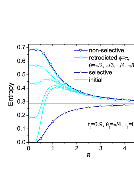
Figure 2: Average entropies corresponding to the qubit retrodicted measurement scheme defined by Eqs. (24) and (25). The entropies are plotted as a function of the parameter $a$ that defines the first measurement. The angles of the second projective measurement are $\phi=\pi$ and, from top to bottom, $\theta=\pi/2,\pi/3,\pi/8,$ and $0.$ The parameters of the initial state $(r_{I},\theta_{I},\phi_{I})$ [Eq. (23)] are indicated in the plot, jointly with its entropy (gray line).

In Fig. 2, for a particular initial condition, we show the entropies associated to the nonselective and selective measurements, $\mathcal{S}[\rho_{\Omega}]$ and $\int_{-\infty}^{+\infty}dVp(V)\mathcal{S}[\rho_{V}]$ respectively, as well as the average entropy of the retrodicted smoothed state, $\sum_{y=\pm}p(y)\mathcal{S}[\rho_{y}].$ Consistently, we observe that, independently of the parameter $a$ and angles $(\theta,\phi)$ that define the first and second measurements respectively [Eqs. (24) and (25)], the inequalities (10) are fulfilled.

In the limit $a\rightarrow\infty$ (weak measurement) all entropies converge to the same value, which is given by the entropy of the initial state (gray line). In fact, in this limit all states $\rho_{V}$ are the same [Eq. (28)], property that guarantees the equality of all (average) entropies in Eq. (10).

In the limit $a\rightarrow 0$ the first measurement corresponds to a strong projective one in the basis $\{|\pm\rangle\}$ of eigenstates of $\sigma_{z}.$ When $\theta=0,$ and arbitrary $\phi,$ the second projective measurement is performed in the same basis $\{|\pm\rangle\}.$ Thus, both measurement outcomes are completely correlated, which leads to the equality of the average entropies of the selective and retrodicted measurements. On the other hand, for $\theta=\pi/2,$ $\phi=\pi,$ the second measurement is performed in the basis of eigenstates of $\sigma_{x}.$ In this case, both measurement outcomes are statistically independent (see Appendix A), which leads to the equality of the average entropies of the non-selective and retrodicted measurements. While the previous properties are strictly fulfilled for $a=0,$ in Fig. 2 they remain approximately valid for $0\leq a\leq a_{s}\approx 0.4.$ Thus, from an entropic point of view, in that interval the first measurement may be considered as a projective one. In fact, in all curves of Fig. 2, the value of the plateau regime around the origin can be estimated by taking into account two successive projective measurements, the first one being in the $z$-direction and the second one in the direction defined by the angles $(\theta,\phi).$

Post-selected expectation values and entropies

Under post-selection murch , the measurement defined by the operator (24) leads to the so-called weak values weak . Here, this feature is analyzed from an entropic point of view.

From the retrodicted measurement scheme it is possible to define the averages

$$\langle V_{\Omega}\rangle\equiv\int_{-\infty}^{+\infty}dVVp(V),\ \ \ \ \ \ \ \langle V_{\pm}\rangle\equiv\int_{-\infty}^{+\infty}dVVp(V|\pm).$$ (32)

Here, $\langle V_{\Omega}\rangle$ gives the (unconditional) average of (the random variable) $V$ associated to the first measurement. On the other hand, $\langle V_{\pm}\rangle$ is the (conditional) average of $V$ given that the second measurement outcomes is $y=\pm.$ In agreement with Eq. (9), they fulfill the relation $\langle V_{\Omega}\rangle=p(+)\langle V_{+}\rangle+p(-)\langle V_{-}\rangle.$ Furthermore, from Eq. (27) it follows $\langle V_{\Omega}\rangle=\langle+|\rho_{I}|+\rangle-\langle-|\rho_{I}|-\rangle=\mathrm{Tr}[\rho_{I}\sigma_{z}]=r_{I}\cos(\theta_{I}).$ Consistently, anomalous weak values are defined by the condition $|\langle V_{\pm}\rangle|>1.$

In Fig. 3(a) and (b) we show the behavior of $\langle V_{\pm}\rangle$ as a function of the parameter $a.$ As expected, by increasing the parameter $a$ (weak measurement limit) the anomalous property $|\langle V_{\pm}\rangle|>1$ may develops. Furthermore, we find that this feature is absent for $0\leq a\leq a_{s}\approx 0.4,$ which correspond to the interval where, from an entropic point of view, the first measurement can be approximated by a strong projective one (plateaus in Fig. 2).

Similarly to expectation values, one can define the conditional entropies $\mathcal{S}[\rho_{\pm}],$ which correspond to the entropies of each post-selected smoothed state, Eq. (31). For the same parameters values, these objects are shown in Fig. 3(c) and (d). We find that $\mathcal{S}[\rho_{\pm}]$ do not fulfill the (average) bounds (10). In addition, we deduce that this feature cannot be related with the anomalous property of the weak expectation values. In fact, in general, any relation may occur, that is, normal or anomalous weak values may develop while the corresponding conditional entropies may or not be bounded by the constraints (10).

V.2 Retrodiction in a bipartite quantum-classical optical-like hybrid system

Retrodiction was studied in different physical arranges where the effective dynamics can be described through a quantum system $(A)$ coupled to unobservable stochastic classical degrees of freedom $(B)$ tsang . The quantum system is continuously monitored in time. For optical ones, its fluorescence signal is observed via photon- or homodyne-detection processes wiseman ; retro . In Ref. molmer , the state of the (two-state) classical system randomly modulate the coherent (fluorescent intensity) system dynamics. In general, one may also consider situations where the classical subsystem modulate any of the characteristic parameters of the quantum evolution sms . These hybrid dynamics can also be studied from the present perspective, that is, through the entropic inequality Eq. (10) and the mutual information inequalities Eqs. (19) and (20).

We consider a hybrid quantum-classical system whose initial bipartite state is

$$\rho_{I}^{ab}=\sum_{\mu}q_{\mu}\rho_{\mu}\otimes|c_{\mu}\rangle\langle c_{\mu}|.$$ (33)

Here, $\{\rho_{\mu}\}$ are different states $(\mathrm{Tr}_{a}[\rho_{\mu}]=1)$ of a quantum two-level system $A,$ while the projectors $\{|c_{\mu}\rangle\langle c_{\mu}|\}$ represent different (countable) macrostates of classical system $B.$ Their statistical weights satisfy $\sum_{\mu}q_{\mu}=1.$ The states $\{\rho_{\mu}\}$ are written as

$$\rho_{\mu}=\frac{1}{2}(\mathrm{I}+\mathbf{r}_{\mu}\cdot\mathbf{\sigma}),$$ (34)

where, similarly to Eq. (23), $\{\mathbf{r}_{\mu}\}$ are Bloch vectors. Hence, $\rho_{\mu}=\rho_{\mu}(r_{\mu},\theta_{\mu},\phi_{\mu}).$

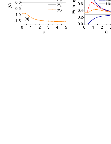
Figure 3: (a)-(b) Unconditional and conditional expectations values [Eq. 32] as a function of the parameter $a.$ (c)-(d) Conditional entropies of the post-selected (smoothed) states [Eq. (31)] jointly with the upper and lower bounds corresponding to non-selective and selective measurements respectively. In (a)-(c), the parameters are $(\theta,\phi)=(\pi/4,\pi)$ while the initial condition is defined by $(r_{I},\theta_{I},\phi_{I})=(0.9,\pi/4,0).$ In (b)-(d), the parameters are $(\theta,\phi)=(\pi/6,0),$ with initial condition $(r_{I},\theta_{I},\phi_{I})=(0.9,\pi/2,0).$

The first (projective) measurement is defined by the operators $(m\rightarrow\mu)$

$$\Omega_{\mu}=|c_{\mu}\rangle\langle c_{\mu}|,$$ (35)

which are associated to each classical macrostate. The operators of the second measurement are $(y=\pm)$

$$M_{+}=|-\rangle\langle+|,\ \ \ \ \ \ \ \ \ M_{-}=|-\rangle\langle-|,$$ (36)

where, as before, $|\pm\rangle$ are the eigenstates of $\sigma_{z},$ and $M_{+}^{{\dagger}}M_{+}+M_{-}^{{\dagger}}M_{-}=\mathrm{I.}$ This generalized measurement nielsen can straightforwardly be read as a photon-detection process. In fact, $M_{+}$ and $M_{-}$ can be associated to the presence and absence of a transition $|+\rangle\rightsquigarrow|-\rangle,$ that is, a photon-detection event. The previous definitions completely set the retrodicted measurement scheme of Fig. 1.

The state of the bipartite system after a measurement performed with the operators $\{\Omega_{\mu}\},$ in a selective and non-selective ways, respectively lead to [Eqs. (1) and (6)]

$$\rho_{\mu}^{ab}=\rho_{\mu}\otimes|c_{\mu}\rangle\langle c_{\mu}|,\ \ \ \ \ \ \ \ \ \ \rho_{\Omega}^{ab}=\rho_{I}^{ab}.$$ (37)

The first expression say us that $\rho_{\mu}$ is the state of $A$ given that $B$ is in the macrostate $\mu.$ Similarly to the experimental situations quoted previously, the second equality represent the inaccessibility of the classical degrees of freedom.

Using that $M_{+}^{{\dagger}}M_{+}=|+\rangle\langle+|$ and $M_{-}^{{\dagger}}M_{-}=|-\rangle\langle-|,$ the joint probabilities Eq. (3) $[p(y,m)\rightarrow p(\pm,\mu)]$ read

$$p(\pm,\mu)=q_{\mu}\langle\pm|\rho_{\mu}|\pm\rangle=q_{\mu}\frac{1}{2}[1\pm r_{\mu}\cos(\theta_{\mu})].$$ (38)

This expression in turn allows us to calculate the retrodicted probabilities $\{p(\mu|\pm)\}$ [Eq. (5)] and $p(\pm)$ [Eq. (4)]. The retrodicted smoothed state read [Eq. (7)]

$$\rho_{\pm}^{ab}=\sum_{\mu}p(\mu|\pm)\rho_{\mu}\otimes|c_{\mu}\rangle\langle c_{\mu}|.$$ (39)

Notice that in contrast with projective measurements in arbitrary bipartite systems [Eq. (18)], here the smoothed state only differs from the initial condition [Eq. (33)] by the replacement $q_{\mu}\rightarrow p(\mu|\pm).$ A similar result was found in Ref. retro .

In order to exemplify the problem we consider a two-state classical system, $\mu=1,2.$ Therefore, the free parameters are $(r_{1},\theta_{1},\phi_{1}),$ $(r_{2},\theta_{2},\phi_{2}),$ for the initial states $\{\rho_{\mu}\}_{\mu=1,2},$ while an extra parameter $q$ gives their weights in the initial bipartite state (33), $q_{1}=q$ and $q_{2}=(1-q).$ Explicit expressions for the entropies and mutual information can be read from Appendix C.

In Fig. 4(a), for a set of particular initial conditions, we plot the entropy of the quantum subsystem $A$ as a function of the weight $q.$ Consistently, as demonstrated in Sec. III, the inequalities (10) are fulfilled by the entropies of the subsystem. In Fig. 4(b) we show the dependence of the (average) mutual information for the non-selective, retrodicted and selective measurements schemes. In agreement with Eqs. (19) and (20), we observe that, while the retrodicted scheme implies an entropic benefit for each subsystem, the retrodicted measurement decreases their mutual information when compared with the non-selective measurement. The difference between these objects is measured by the retrodicted-like Holevo bound (22). On the other hand, the average mutual information for the selective measurement vanishes [see Eq. (37)]. The main features shown in Fig. 4 remain valid for arbitrary initial conditions.

Figure 4: (a) Entropy of the quantum subsystem for the measurement scheme defined by Eqs. (35) and (36). (b) Mutual information of the quantum-classical arrange. The parameter $q$ define the weights of the initial bipartite state Eq. (33). The states of the quantum subsystem $(\rho_{1}$ and $\rho_{2})$ [Eq. (34)] are defined with $(r_{1},\theta_{1},\phi_{1})=(0,0,0),$ and $(r_{2},\theta_{2},\phi_{2})=(1,0,0).$

VI Summary and Conclusions

We performed and informational-entropic study of retrodicted quantum measurements (Fig. 1). Given that a non-selective measurement was performed over a system of interest, a second successive measurement is used for improving the estimation of the possible outcomes of the former one. From the quantum expressions for the outcome probabilities, Bayes rule allows to obtaining the corresponding retrodicted probabilities, Eq. (5). The system state after the retrodicted measurement (smoothed state) results from an addition of the system transformations associated to each measurement outcome with a weight given by the retrodicted probabilities, Eq. (7).

Based on the concavity of von Neumann entropy we proved that, in average, the entropy of the smoothed state is bounded from above and below by the entropies associated to the first non-selective measurement and the entropy corresponding to its selective resolution respectively, Eq. (10). This central result quantifies how much information gain may be obtained from the retrodicted measurement scheme.

For bipartite systems it was shown that, independently of the measurements nature, the same property is valid for the entropy of each subsystem. In addition, based on the strong subadditivity of von Neumann entropy, upper bounds for the mutual information changes were also established, Eqs. (13) and (14).

We specified the previous results for a bipartite system where the measurements are performed over each single system successively, being projective the former one. The retrodicted measurement diminishes the entropy of each subsystem. Nevertheless, their (average) mutual information is diminished with respect to that of the non-selective measurement, Eq. (19). This reduction is bounded from below by the (average) mutual information of the selective resolution of the first measurement, Eq. (20). These inequalities in turn lead to a kind of retrodicted Holevo inequality that bound the (classical) mutual information [Eq. (22)] between the two sets of measurement outcomes.

As explicit examples we worked out the case of a qubit subjected to weak and strong retrodicted measurements. All theoretical results are confirmed by the model. In addition, we find that anomalous weak values arise when, from an entropic point of view, the first measurement cannot be approximated by a strong projective one. On the other hand, we considered a bipartite quantum-classical optical-like hybrid system. Degradation of mutual information under the retrodicted measurement scheme was explicitly confirmed.

The developed results quantify the information changes that follow from a retrodicted measurement. While the entropy of the system of interest is always diminished, implying an information vantage, in bipartite systems mutual information may be degraded. These results provide a solid basis for studying other informational measures that may be of interest is physical arrangements where retrodicted measurements are implemented.

Appendix A Demonstration of entropy inequalities

The entropy inequalities for the retrodicted measurement scheme can be derived as follows. They rely on the concavity of the von Neumann entropy nielsen , $\mathcal{S}[\sum_{k}p(k)\rho_{k}]\geq\sum_{k}p(k)\mathcal{S}[\rho_{k}],$ with equality if and only if all states $\rho_{k}$ for which $p(k)>0$ are identical. Starting from the $\mathcal{S}[\sum_{m}p(m)\rho_{m}],$ and using Eq. (9), it leads to the following inequalities

$$\mathcal{S}\Big{[}\sum_{m}p(m)\rho_{m}\Big{]}\!\! = \!\!\mathcal{S}\Big{[}\sum_{y}p(y)\rho_{y}\Big{]}\geq\sum_{y}p(y)\mathcal{S}[\rho_{y}],\ \ \ \ \ \ \$$ (40a)

$$= \!\sum_{y}p(y)\mathcal{S}\Big{[}\sum_{m}p(m|y)\rho_{m}\Big{]},\ \$$ (40b)

$$\geq \!\sum_{y}p(y)\sum_{m}p(m|y)\mathcal{S}[\rho_{m}],$$ (40c)

$$= \!\sum_{y}\sum_{m}p(m,y)\mathcal{S}[\rho_{m}],$$ (40d)

$$= \!\sum_{m}p(m)\mathcal{S}[\rho_{m}],$$ (40e)

where we have used that $$p(m)=\sum_{y}p(m,y)=\sum_{y}p(m|y)p(y).$$ Taking into account the first and last lines, it follows

$$\mathcal{S}\Big{[}\sum_{m}p(m)\rho_{m}\Big{]}\geq\sum_{y}p(y)\mathcal{S}[\rho_{y}]\geq\sum_{m}p(m)\mathcal{S}[\rho_{m}],$$ (41)

which recovers the entropy inequalities (10).

Given that equality in the concavity entropy inequality is valid if and only if all states with nonvanishing weight are the same, from Eq. (40a) we deduce that the upper bound is achieved when all states $\{\rho_{y}\}$ are the same. This condition happens when all states $\{\rho_{m}\}$ are identical, or alternatively when $p(m|y)=p(m)$ [see definition (7)]. Hence, the joint probability Eq. (3) satisfies $p(y,m)=p(y)p(m).$ This condition implies that both measurement results, $\{m\}$ and $\{y\},$ are statistically independent. This property is fulfilled by projective measurements $\Omega_{m}=|m\rangle\langle m|$ and $M_{y}=|y\rangle\langle y|,$ where the basis of states $\{|m\rangle\}$ and $\{|y\rangle\}$ are such that $|\langle m|y\rangle|^{2}$ is independent of $m$ nota1 .

Similarly, from Eq. (40c) we deduce that the lower bound in Eq. (41) is achieved when all states $\{\rho_{m}\}$ are the same, or alternatively when $p(m|y)=\delta_{my}.$ Hence, the joint probability Eq. (3) satisfies $p(y,m)=\delta_{my}p(y)=\delta_{ym}p(m),$ that is, both measurement results, $\{m\}$ and $\{y\},$ are completely correlated. From Eq. (3), we deduce that this condition is fulfilled by projective measurements $\Omega_{m}=|m\rangle\langle m|$ and $M_{y}=|y\rangle\langle y|,$ where the basis of states $\{|m\rangle\}$ and $\{|y\rangle\}$ are the same, $|\langle m|y\rangle|^{2}=\delta_{my}.$

We notice that statistical independence and complete correlation between both measurement outcomes also give the equality conditions for the entropies of the measurement probabilities $\{p(m)\}$ and their retrodicted version $\{p(m|y)\}.$ They satisfy the classical inequality nielsen

$$\mathcal{H}[m]\geq\mathcal{H}[m|y]\geq 0,$$ (42)

where $\mathcal{H}[m]=-\sum_{m}p(m)\ln[p(m)]$ and $\mathcal{H}[m|y]=-\sum_{y}p(y)\sum_{m}p(m|y)\ln[p(m|y)]$ is the conditional Shannon entropy of outcomes $\{m\}$ given outcomes $\{y\}.$ In fact, $\mathcal{H}[m]=\mathcal{H}[m|y]$ when $p(y,m)=p(y)p(m)$ nielsen . On the other hand, the lower bound $\mathcal{H}[m|y]=0$ occurs when $\{m\}$ is a deterministic function of $\{y\}$ nielsen , which here corresponds to $p(y,m)=\delta_{my}p(y)=\delta_{ym}p(m).$

By using the upper bound nielsen $\sum_{k}p(k)\mathcal{S}[\rho_{k}]+\mathcal{H}[k]\geq\mathcal{S}[\sum_{k}p(k)\rho_{k}],$ with equality if and only if all states $\rho_{k}$ have support on orthogonal subspaces, where $\mathcal{H}[k]=-\sum_{k}p(k)\ln[p(k)],$ under the replacement $k\rightarrow y$ it follows

$$\mathcal{H}[y]\geq\mathcal{S}\Big{[}\sum_{y}p(y)\rho_{y}\Big{]}-\sum_{y}p(y)\mathcal{S}[\rho_{y}].$$ (43)

Taking into account that $\sum_{y}p(y)\rho_{y}=\sum_{m}p(m)\rho_{m}$ [Eq. (9)], the previous expression recovers Eq. (11). This upper bound is achieved when all states $\{\rho_{y}\}$have support on orthogonal subspaces. On the other hand, taking $k\rightarrow m$ the upper entropy bound becomes

$$\mathcal{H}[m] \geq \mathcal{S}\Big{[}\sum_{m}p(m)\rho_{m}\Big{]}-\sum_{m}p(m)\mathcal{S}[\rho_{m}],\ \ \ \$$ (44a)

$$\geq \sum_{y}p(y)\mathcal{S}[\rho_{y}]-\sum_{m}p(m)\mathcal{S}[\rho_{m}],$$ (44b)

where the last inequality is guaranteed by Eq. (41), which in turn recovers Eq. (12). This upper bound is achieved when all states $$\{\rho_{m}\} p(m|y)=p(m).$$ have support on orthogonal subspaces and

Appendix B Demonstration of mutual information inequalities

Here we demonstrate the inequalities that bound the changes in the mutual information of a bipartite arrangement consisting in subsystems $A$ and $B,$ Eqs. (13) and (14). The demonstrations rely on the strong subadditivity property of von Neumann entropy nielsen . Hence, an extra ancilla system $C$ is introduced.

First inequality: The tripartite arrangement is described by the state

$$\rho^{abc}=\sum_{m,y}p(m,y)\rho_{m}^{ab}\otimes|y\rangle\langle y|,$$ (45)

where $p(m,y)$ is an arbitrary joint probability of $m$ and $y.$ Hence, $\sum_{m}p(m,y)=p(y),$ and $\sum_{y}p(m,y)=p(m).$ The set $\{\rho_{m}^{ab}\}$ are states in the $AB$ Hilbert space, $\mathrm{Tr}_{ab}[\rho_{y}^{ab}]=1,$ while $\{|y\rangle\}$ is an orthogonal base of the Hilbert space of $C.$ The marginal state of $AB$ and $C,$ $\rho^{ab}$ and $\rho^{c}$ respectively, read

$$\rho^{ab}=\sum_{m}p(m)\rho_{m}^{ab},\ \ \ \ \ \ \ \rho^{c}=\sum_{y}p(y)|y\rangle\langle y|,$$ (46)

where $\rho^{ab}$ by partial trace defines the states of $A$ and $B,$ $\rho^{a}=\mathrm{Tr}_{b}[\rho^{ab}]$ and $\rho^{b}=\mathrm{Tr}_{a}[\rho^{ab}]$ respectively. The entropy of the tripartite state $\rho^{abc},$ by using that $p(m,y)=p(m|y)p(y),$ can be written as

$$\mathcal{S}[\rho^{abc}]=\mathcal{H}[y]+\sum_{y}p(y)\mathcal{S}[\rho_{y}^{ab}],$$ (47)

where

$$\rho_{y}^{ab}=\sum_{m}p(m|y)\rho_{m}^{ab},$$ (48)

and $\mathcal{H}[y]$ is the classical Shannon entropy of the distribution $\{p(y)\},$ $\mathcal{H}[y]=-\sum_{y}p(y)\ln[p(y)].$ Similarly, the entropies $\mathcal{S}[\rho^{ac}]$ and $\mathcal{S}[\rho^{bc}]$ follows from Eq. (47) under the replacements $\rho_{y}^{ab}\rightarrow\rho_{y}^{a}=\mathrm{Tr}_{b}[\rho_{y}^{ab}]$ and $\rho_{y}^{ab}\rightarrow\rho_{y}^{b}=\mathrm{Tr}_{a}[\rho_{y}^{ab}]$ respectively. Using the strong subadditivity condition $\mathcal{S}[\rho^{abc}]+\mathcal{S}[\rho^{a}]\leq\mathcal{S}[\rho^{ab}]+\mathcal{S}[\rho^{ac}]$ nielsen , it follows

$$\mathcal{S}[\rho^{a}]-\mathcal{S}[\rho^{ab}]\leq\sum_{y}p(y)\mathcal{S}[\rho_{y}^{a}]-\sum_{y}p(y)\mathcal{S}[\rho_{y}^{ab}].$$ (49)

Interchanging the indices $a\leftrightarrow b,$ the previous inequality becomes

$$\mathcal{S}[\rho^{b}]-\mathcal{S}[\rho^{ab}]\leq\sum_{y}p(y)\mathcal{S}[\rho_{y}^{b}]-\sum_{y}p(y)\mathcal{S}[\rho_{y}^{ab}].$$ (50)

The addition of the previous two expressions lead to

$$\mathcal{I}[\rho^{ab}]-\sum_{y}p(y)\mathcal{I}[\rho_{y}^{ab}]\leq\mathcal{S}[\rho^{ab}]-\sum_{y}p(y)\mathcal{S}[\rho_{y}^{ab}],$$ (51)

which recovers Eq. (13), where the mutual information of a bipartite state is $\mathcal{I}[\rho^{ab}]=\mathcal{S}[\rho^{a}]+\mathcal{S}[\rho^{b}]-\mathcal{S}[\rho^{ab}].$

Second inequality: In this case the tripartite arrangement is described by the state

$$\rho_{y}^{abc}=\sum_{m}p(m|y)\rho_{m}^{ab}\otimes|m\rangle\langle m|.$$ (52)

This state parametrically depends on $y.$ $p(m|y)$ is an arbitrary conditional probability of $m$ given $y,$ $\sum_{m}p(m|y)=1.$ The set $\{\rho_{m}^{ab}\}$ are states in the Hilbert space of the bipartite system $AB,$ $\mathrm{Tr}_{ab}[\rho_{y}^{ab}]=1,$ while here $\{|m\rangle\}$ is an orthogonal base of the Hilbert space of $C.$ The marginal state of $AB$ and $C,$ $\rho_{y}^{ab}$ and $\rho_{y}^{c}$ respectively, read

$$\rho_{y}^{ab}=\sum_{m}p(m|y)\rho_{m}^{ab},\ \ \ \ \ \ \rho_{y}^{c}=\sum_{m}p(m|y)|m\rangle\langle m|.$$ (53)

The states of $A$ and $B$ read $\rho_{y}^{a}=\mathrm{Tr}_{b}[\rho_{y}^{ab}]$ and $\rho_{y}^{b}=\mathrm{Tr}_{a}[\rho_{y}^{ab}]$ respectively.

A straightforward calculation leads to

$$\mathcal{S}[\rho_{y}^{abc}]=\mathcal{H}[m]|_{y}+\sum_{m}p(m|y)\mathcal{S}[\rho_{m}^{ab}],$$ (54)

where

$$\mathcal{H}[m]|_{y}\equiv-\sum_{m}p(m|y)\ln[p(m|y)].$$ (55)

The entropies $\mathcal{S}[\rho_{y}^{ac}]$ and $\mathcal{S}[\rho_{y}^{bc}]$ follows from Eq. (54) under the replacements $\rho_{m}^{ab}\rightarrow\rho_{m}^{a}$ and $\rho_{m}^{ab}\rightarrow\rho_{m}^{b}$ respectively.

Using the strong subadditivity condition nielsen $\mathcal{S}[\rho^{abc}]+\mathcal{S}[\rho^{a}]\leq\mathcal{S}[\rho^{ab}]+\mathcal{S}[\rho^{ac}],$ with $\rho^{abc}\rightarrow\rho_{y}^{abc}$ [Eq. (52)], jointly with Eq. (54), lead to

$$\mathcal{S}[\rho_{y}^{a}]-\mathcal{S}[\rho_{y}^{ab}]\leq\sum_{m}p(m|y)\mathcal{S}[\rho_{m}^{a}]-\sum_{m}p(m|y)\mathcal{S}[\rho_{m}^{ab}].$$ (56)

Interchanging $a\leftrightarrow b$ in the strong subadditivity condition, the previous equation becomes

$$\mathcal{S}[\rho_{y}^{b}]-\mathcal{S}[\rho_{y}^{ab}]\leq\sum_{m}p(m|y)\mathcal{S}[\rho_{m}^{b}]-\sum_{m}p(m|y)\mathcal{S}[\rho_{m}^{ab}].$$ (57)

By adding the previous two inequalities, it follows

$$\mathcal{I}[\rho_{y}^{ab}]-\sum_{m}p(m|y)\mathcal{I}[\rho_{m}^{ab}]\leq\mathcal{S}[\rho_{y}^{ab}]-\sum_{m}p(m|y)\mathcal{S}[\rho_{m}^{ab}],$$ (58)

By applying $\sum_{y}p(y)$ to each contribution in the previous inequality, and using that $\sum_{y}p(m|y)p(y)=p(m),$ lead to

$$\sum_{y}p(y)\mathcal{I}[\rho_{y}^{ab}]-\sum_{m}p(m)\mathcal{I}[\rho_{m}^{ab}]$$ (59)

$$\leq \sum_{y}p(y)\mathcal{S}[\rho_{y}^{ab}]-\sum_{m}p(m)\mathcal{S}[\rho_{m}^{ab}],$$

which recovers Eq. (14).

Appendix C Bipartite projective measurements

Here, we apply the main results of Sec. II to the case of bipartite projective measurements presented in Sec. III.

C.1 Entropy inequalities

From Eq. (17), a straightforward calculation gives

$$\mathcal{S}[\rho_{\Omega}^{ab}]=\mathcal{H}[m]+\sum_{m}p(m)\mathcal{S}[\rho_{m}^{a}].$$ (60)

From Eq. (18), the average entropy of the smoothed state reads

$$\sum_{y}p(y)\mathcal{S}[\rho_{y}^{ab}]=\mathcal{H}[m|y]+\sum_{m}p(m)\mathcal{S}[\rho_{m}^{a}],$$ (61)

where $\mathcal{H}[m|y]=-\sum_{y}p(y)\sum_{m}p(m|y)\ln[p(m|y)]=\mathcal{H}[m,y]-\mathcal{H}[y]$ is the conditional entropy of outcomes $\{m\}$ given outcomes $\{y\}.$ From Eq. (16), the average entropy corresponding to the selective resolution of the non-selective measurement is

$$\sum_{m}p(m)\mathcal{S}[\rho_{m}^{ab}]=\sum_{m}p(m)\mathcal{S}[\rho_{m}^{a}].$$ (62)

Using that $0\leq\mathcal{H}[m|y]\leq\mathcal{H}[m]$ nielsen , it follows that the entropy inequalities (10) are fulfilled by the bipartite system.

From Eqs. (60) and (61), jointly with the inequality (11) it follows

$$\mathcal{S}[\rho_{\Omega}^{ab}]-\sum_{y}p(y)\mathcal{S}[\rho_{y}^{ab}]=\mathcal{H}[m:y]\leq\mathcal{H}[y],$$ (63)

where $\mathcal{H}[m:y]=\mathcal{H}[m]-\mathcal{H}[m|y]=\mathcal{H}[m]+\mathcal{H}[y]-\mathcal{H}[m,y],$ is the classical mutual information between the outcomes of both measurements, $\{m\}$ and $\{y\}.$ The demonstration of the inequality $\mathcal{H}[m:y]\leq\mathcal{H}[y]$ can be found in nielsen . In addition, the inequality (12), from Eqs. (61) and (62), reads

$$\sum_{y}p(y)\mathcal{S}[\rho_{y}^{ab}]-\sum_{m}p(m)\mathcal{S}[\rho_{m}^{ab}]=\mathcal{H}[m|y]\leq\mathcal{H}[m].$$ (64)

The demonstration of the inequality $0\leq\mathcal{H}[m|y]\leq\mathcal{H}[m]$ can also be found in nielsen . The previous two equations demonstrate that the general inequalities (11) and (12) are in fact fulfilled.

In the previous expressions the probabilities read $p(m)=\mathrm{Tr}_{a}[\langle m|\rho_{I}|m\rangle]$ [Eq. (1)]. Furthermore, $p(y|m)=\mathrm{Tr}_{a}[M_{y}^{\dagger}M_{y}\rho_{m}^{a}]$ [Eq. (2)], $p(y,m)=\mathrm{Tr}_{a}[\langle m|\rho_{I}|m\rangle M_{y}^{\dagger}M_{y}]$ [Eq. (3)], while the retrodicted probability $p(m|y)$ [Eq. (5)] reads $p(m|y)=\mathrm{Tr}_{a}[\langle m|\rho_{I}|m\rangle M_{y}^{\dagger}M_{y}]/p(y)$ where $p(y)=\sum_{m}\mathrm{Tr}_{a}[\langle m|\rho_{I}|m\rangle M_{y}^{\dagger}M_{y}]$ [Eq. (4)].

Subsystems: The previous results can also be specified for subsystem $A$ and $B.$ From Eqs. (17) and (18), it follows $\rho_{\Omega}^{b}=\sum_{m}p(m)|m\rangle\langle m|,$ and $\rho_{y}^{b}=\sum_{y}p(m|y)|m\rangle\langle m|.$ Furthermore, $\rho_{m}^{b}=|m\rangle\langle m|.$ The inequality Eq. (10), specified for subsystem $B,$ becomes $\mathcal{S}[\rho_{\Omega}^{b}]=\mathcal{H}[m]\geq\sum_{y}p(y)\mathcal{S}[\rho_{y}^{b}]=\mathcal{H}[m|y]\geq\sum_{m}p(m)\mathcal{S}[\rho_{m}^{b}]=0,$ because $\mathcal{S}[\rho_{m}^{b}]=0.$ Hence, $\mathcal{H}[m]\geq\mathcal{H}[m|y]\geq 0,$ which is a well known inequality valid for Shannon entropies nielsen . Instead for subsystem $A,$ Eq. (10) leads to the non-trivial relation

$$\mathcal{S}[\rho_{\Omega}^{a}]\geq\sum_{y}p(y)\mathcal{S}[\rho_{y}^{a}]\geq\sum_{m}p(m)\mathcal{S}[\rho_{m}^{a}],$$ (65)

where $\rho_{\Omega}^{a}=\sum_{m}p(m)\rho_{m}^{a}$ and $\rho_{y}^{a}=\sum_{y}p(m|y)\rho_{m}^{a}$ [see Eqs. (17) and (18)]. This inequality say us that while the first measurement is performed over subsystem $B,$ an information gain is also guaranteed for subsystem $A.$

The inequalities (11) and (12) can also be specified for each subsystem. For subsystem $A$ they become $\mathcal{S}[\rho_{\Omega}^{a}]-\sum_{y}p(y)\mathcal{S}[\rho_{y}^{a}]\leq\mathcal{H}[y],$ and $\sum_{y}p(y)\mathcal{S}[\rho_{y}^{a}]-\sum_{m}p(m)\mathcal{S}[\rho_{m}^{a}]\leq\mathcal{H}[m].$ For subsystem $B$ they lead to the same classical entropic relations found previously.

C.2 Mutual information inequalities

The mutual information under the different measurement schemes are characterized by Eqs. (13) and (14). Each term appearing in these inequalities is explicitly calculated below.

From the entropy expressions (60), (61), and (62), the mutual information associated to the different measurement stages read

$$\mathcal{I}[\rho_{\Omega}^{ab}]=\mathcal{S}[\rho_{\Omega}^{a}]-\sum_{m}p(m)\mathcal{S}[\rho_{m}^{a}],$$ (66)

while

$$\sum_{y}p(y)\mathcal{I}[\rho_{y}^{ab}]=\sum_{y}p(y)\mathcal{S}[\rho_{y}^{a}]-\sum_{m}p(m)\mathcal{S}[\rho_{m}^{a}].$$ (67)

The difference of the previous two equations leads to the lower bound of Eq. (19). On the other hand, from Eq. (16) it follows $\sum_{m}p(m)\mathcal{I}[\rho_{m}^{ab}]=0,$ which in turn lead to the lower bound of Eq. (20).

The upper bounds of Eqs. (19) and (20) follows from the general inequalities (13) and (14) written in terms of Eqs. (63) and (64) respectively.

References

- (1) M. A. Nielsen and I. L. Chuang, Quantum Computation and Quantum Information (Cambridge University Press, Cambridge, England, 2000).
- (2) H. P. Breuer and F. Petruccione, The theory of open quantum systems, (Oxford University press, 2002).
- (3) Y. Aharonov, P. G. Bergman, and J. L. Lebowitz, Time symmetry in the quantum process of measurement, Phys. Rev. 134, B1410 (1964); Y. Aharonov and D. Z. Albert, Is the usual notion of time evolution adequate for quantum-mechanical systems?, Phys. Rev. D 29, 223 (1984); Y. Aharonov and D. Z. Albert, Is the usual notion of time evolution adequate for quantum-mechanical systems? II. Relativistic considerations, Phys. Rev. D 29, 228 (1984).
- (4) Y. Aharonov and L. Vaidman, Properties of a quantum system during the time interval between two measurements, Phys. Rev. A 41,11 (1990); Y. Aharonov and L. Vaidman, Complete description of a quantum system at a given time, J. Phys. A: Math. Gen. 24, 2315 (1991).
- (5) S. Gammelmark, B. Julsgaard, and K. Mølmer, Past Quantum States of a Monitored System, Phys. Rev. Lett. 111, 160401 (2013).
- (6) I. Guevara and H. Wiseman, Quantum State Smoothing, Phys. Rev. Lett. 115, 180407 (2015).
- (7) M. Tsang, Time-symmetric quantum theory of smoothing, Phys. Rev. Lett. 102, 250403 (2009).
- (8) A. H. Jazwinski, Stochastic Processes and Filtering Theory (Academic Press, New York, 1970).
- (9) W. H. Press, S. A. Teukolsky, W. T. Vetterling, and B. P. Flannery, Numerical Recipes: The Art of Scientific Computing, 3rd ed. (Cambridge University Press, New York, 2007).
- (10) H. M. Wiseman and G. J. Milburn, Quantum Measurement and Control (Cambridge University press, 2010).
- (11) H. J. Carmichael, An Open Systems Approach to Quantum Optics, Lecture Notes in Physics, Vol. M18 (Springer, Berlin, 1993); M. B. Plenio and P. L. Knight, The quantum-jump approach to dissipative dynamics in quantum optics, Rev. Mod. Phys. 70, 101 (1998).
- (12) M. Tsang, Optimal waveform estimation for classical and quantum systems via time-symmetric smoothing, Phys. Rev. A 80, 033840 (2009); M. Tsang, Optimal waveform estimation for classical and quantum systems via time-symmetric smoothing. II. Applications to atomic magnetometry and Hardy’s paradox, Phys. Rev. A 81, 013824 (2010); M. Tsang, H. M. Wiseman, and C. M. Caves, Fundamental quantum limit to waveform estimation, Phys. Rev. Lett. 106, 090401 (2011).
- (13) S. Gammelmark, K. Mølmer, W. Alt, T. Kampschulte, and D. Meschede, Hidden Markov model of atomic quantum jump dynamics in an optically probed cavity, Phys. Rev. A 89, 043839 (2014).
- (14) D. Tan, S. J. Weber, I. Siddiqi, K. Mølmer, and K. W. Murch, Prediction and Retrodiction for a Continuously Monitored Superconducting Qubit, Phys. Rev. Lett. 114, 090403 (2015).
- (15) T. Rybarczyk, B. Peaudecerf, M. Penasa, S. Gerlich, B. Julsgaard, K. Mølmer, S. Gleyzes, M. Brune, J. M. Raimond, S. Haroche, and I. Dotsenko, Forward-backward analysis of the photon-number evolution in a cavity, Phys. Rev. A 91, 062116 (2015).
- (16) Q. Xu, E. Greplova, B. Julsgaard, and K. Mølmer, Correlation functions and conditioned quantum dynamics in photodetection theory, Phys. Scr. 90, 128004 (2015).
- (17) D. Tan, M. Naghiloo, K. Mølmer, and K. W. Murch, Quantum smoothing for classical mixtures, Phys. Rev. A 94, 050102(R) (2016).
- (18) N. Foroozani, M. Naghiloo, D. Tan, K. Mølmer and K. W. Murch, Correlations of the Time Dependent Signal and the State of a Continuously Monitored Quantum System, Phys. Rev. Lett. 116, 110401 (2016).
- (19) P. Campagne-Ibarcq, L. Bretheau, E. Flurin, A. Auffèves, F. Mallet, and B. Huard, Observing Interferences between Past and Future Quantum States in Resonance Fluorescence, Phys. Rev. Lett. 112, 180402 (2014).
- (20) D. Tan, N. Foroozani, M. Naghiloo, A. H. Kiilerich, K. Mølmer, and K. W. Murch, Homodyne monitoring of postselected decay, Phys. Rev. A 96, 022104 (2017).
- (21) A. A. Budini, Smoothed quantum-classical states in time-irreversible hybrid dynamics, Phys. Rev. A 96, 032118 (2017).
- (22) T. Pegg and S. M. Barnett, Retrodiction in quantum optics, J. Opt. B: Quantum and Semiclass. Opt. 1, 442 (1999); S. M. Barnett and D. T. Pegg, Optical state truncation, Phys. Rev. A 60, 4965 (1999); S. M. Barnett, D. T. Pegg, and J. Jeffers, Bayes’ Theorem and quantum retrodiction, J. Mod. Opt. 47, 1779 (2000); S. M. Barnett, D. T. Pegg, J. Jeffers, and O. Jedrkiewicz, Atomic retrodiction, J. Phys. B: At. Mol. Opt. Phys. 33, 3047 (2000); S. M. Barnett, D. T. Pegg, J. Jeffers, O. Jedrkiewicz, and R. Loudon, Retrodiction for quantum optical communications, Phys. Rev. A 62, 022313 (2000).
- (23) S. M. Barnett, D. T. Pegg, J. Jeffers, and O. Jedrkiewicz, Master equation for retrodiction of quantum communication signals, Phys. Rev. Lett. 86, 2455 (2001); D. T. Pegg, S. M. Barnett, and J. Jeffers, Quantum retrodiction in open systems, Phys. Rev. A 66, 022106 (2002).
- (24) P. Hayden, R. Jozsa, D. Petz, and A. Winter, Structure of states which satisfy strong subadditivity of quantum entropy with equality, Comm. Math. Phys. 246, 359 (2003); A. Wehrl, General properties of entropy, Rev. Mod. Phys. 50, 221 (1978).
- (25) J. Dressel, M. Malik, F. M. Miatto, A. N. Jordan, and R. W. Boyd, Understanding quantum weak values: Basics and applications, Rev. Mod. Phys. 86, 307 (2014).
- (26) A. A. Budini, Quantum jumps and photon statistics in fluorescent systems coupled to classically fluctuating reservoirs, J. Phys. B 43, 115501 (2010); A. A. Budini, Open quantum system approach to single-molecule spectroscopy, Phys. Rev. A 79, 043804 (2009).
- (27) This occurs, for example, for a qubit system where the measurements operators are and where and are the eigenvectors of the and Pauli matrixes respectively.