Cosmological Parameters For Spatially Flat Dust Filled Universe In Brans-Dicke Theory

Abstract

In this paper, we have investigated late time acceleration for a spatially flat dust filled Universe in Brans-Dicke theory in the presence of a positive cosmological constant $\Lambda$ . Expressions for Hubble’s constant, luminosity distance and apparent magnitude have been obtained for our model. The theoretical results are compared with the observed values of the the latest 287 high red shift ($.3\leq z\leq 1.4$ ) SN Ia supernova data’s taken from Union 2.1 compilation to estimate the present values of the matter and dark energy parameters $(\Omega_{m})_{0}$ and $(\Omega_{\Lambda})_{0}$. We have also estimated the present value of Hubble’s constant $H_{0}$ in the light of a updated sample of Hubble parameter measurements including 19 independent data points. The results are found to be in good agreement with recent astrophysical observations. We have also calculated various physical parameters such as the matter and dark energy densities, the present age of the universe and deceleration parameter. The value for BD-coupling constant $\omega$ is set to be 40000 on the basis of accuracy of the solar system tests and recent experimental evidence.

1 Introduction

The two independent groups headed by Riess and Perlmutter via type Ia supernovae (SNeIa ) (Riess at el  [1997]; Perlmutter at el [1998]), found that our universe is accelerating at present. Several theories have been put forward to explain this remarkable discovery (Spergel et al. [2003]; Bennett et al. [2003];Tegmark et al. [2004]). An exotic bizarre form of the energy called as dark energy is proposed to understand the accelerating expansion. The dark energy is expected to possess a negative pressure, which detracts matters from each other and creates acceleration in the universe. The simplest candidate of dark energy is the positive cosmological constant $\Lambda$ which is considered as a source with equation of state  $p_{\Lambda}=-\rho_{\Lambda}$. The standard Friedmann Robertson Walker ( FRW) model of the universe with cosmological constant as a source of dark energy is often known as $\Lambda$-CDM cosmological model ( Copeland at el.  [2007]; Gron and Hervik [2007]). Basically, the standard FRW model represents decelerating universe but presence of cosmological constant as a source and its specific value makes the model accelerating. It is found that the $\Lambda$-CDM model is in good agreement with latest observations (Abazajian et al. [2004]; Sahni and Starobinsky [2000]). Recently Goswami at el. ( [2015];[2016];[2016]) have developed $\Lambda$-CDM type models for Bianch type I anisotropic universe.
Apart from $\Lambda$-CDM cosmological model, alternative explanations for the accelerated expansion in terms of scalar fields like quintessence ( Caldwell at el [1998]) , K-essence ( Chiba at el.  [2000]) , phantom fields (Caldwell  [2002]) and Chaplin gas (Kamenshchik at el.  [2001]) are available, a number of models involving the cosmological term, especially time-varying Λ have been proposed ( Carvalho at el. [1992]; Wetterich [1995]; Arbab [1997]; Padmanabhan  [2001]; Vishwakarma [2002]; Shapiro and Sola [2004]; Dutta Choudhury and Sil  [2006]).
It is worth to investigate effect of cosmological ‘constant’ in the Brans-Dicke theory of gravity ( Brans and Dicke  [1961]) which describe evolution of the universe that explain accelerating phase of expansion in the current epoch. In a recent paper, Hrycyna and lowski  ([2013]) compared dynamical evolution of the standard cosmological model from the view of both Brans-Dicke and general theory of relativity. Singh and Singh  ([1984]) investigated a cosmological model in Brans-Dicke theory by considering cosmological “constant” as function of scalar field $\phi$. Pimentel  ([1985]) obtained exact cosmological solutions in Brans-Dicke theory with uniform cosmological “constant”. A class of flat FRW cosmological models with cosmological “constant” in Brans-Dicke theory have also been obtained by Azar and Riazi ( [1995]). The age of the universe from a view point of the nucleosynthesis with Λ term in Brans-Dicke theory was investigated by Etoh et al  ([1997]). Azad and Islam ( [2003]) extended the idea of Singh and Singh ( [1984]) to study cosmological constant in Bianchi type I modified Brans-Dicke cosmology. Recently Qiang et al ( [2005]) discussed cosmic acceleration in five dimensional Brans-Dicke theory using interacting Higgs and Brans-Dicke fields. Smolyakov ( [2011]) investigated a model which provides the necessary value of effective cosmological “constant” at the classical level. Embedding general relativity with varying cosmological term in five dimensional Brans-Dicke theory of gravity in vacuum has been discussed by Reyes et al ( [2002]).
In this paper, we have investigated late time acceleration for a spatially flat dust filled Universe in Brans-Dicke theory in the presence of a positive cosmological constant $\Lambda$ . The paper is organized as follows: In section 2, The BD-field equations are developed for a universe filled with cosmic fluid as source of matter in spatially homogeneous and isotropic space-time . In Section 3, we have obtained expression for Gravitational constant in term of red shift by solving BD-field equations. The value for Coupling constant $\omega$ is set to be 40000 on the basis of accuracy of the solar system tests and recent experimental evidence. In this section, we have also obtained expression for Hubble’s constant and relation ship between energy parameters $\Omega_{m}$ and $\Omega_{\Lambda}$. In section 4, expressions for Luminosity distance and apparent magnitude have been obtained . The estimation of energy parameters and Hubble’s constant at present are dealt in the Section 5 and 6. In Section 7, we have obtained various physical parameters such as the matter and dark energy densities, present age of the universe and value of deceleration parameter on the basis of values of $(\Omega_{m})_{0}$, $(\Omega_{\Lambda})_{0}$ & $H_{0}$ obtained by us. The model predicts that acceleration in the universe had begun in the past at $z_{c}=0.6818\thicksim 7.2371\times 10^{9}yrs$ before from present. Finally the conclusions of the paper are presented in section 8. The results of our investigation are consistence with the latest large scale structure measurements by surveys like BOSS, wiggleZ and BAO, and WMAP or Planck results for CMB anisotropies ( Ade et al.  [2016]; Ade et al.  [2013]; Aubourg at el [2015]; Anderson at el  [2014]; Delubac et al. [2015]; Blake et al.  [2012]). WMAP quoted the value of dark energy densities, $\Omega_{\Lambda}$ = $0.7184$, where as the combined WMAP+CMB+BAO+BOSS surveys put $\Omega_{\Lambda}$ = $0.7181$. We have obtained $\Omega_{\Lambda}$ = $0.704$.

2 BD-Field Equation

BD field equations are obtained from following action

$$\delta\int\sqrt{-g}\left\{\phi\left(R-2\Lambda\right)+\omega\frac{\phi_{k}\phi^{k}}{\phi}\right\}$$ (1)

The field equations are

$$R_{ij}-\frac{1}{2}R+\Lambda g_{ij}=-\frac{8\pi}{\phi c^{4}}T_{ij}-\frac{\omega}{\phi^{2}}\left(\phi_{i}\phi_{j}-\frac{1}{2}g_{ij}\phi_{k}\phi^{k}\right)-\frac{1}{\phi}\left(\phi_{i;j}-g_{ij}\Box\phi\right)$$ (2)

$$(2\omega+3)\Box\phi=\frac{8\pi T}{c^{4}}+2\Lambda\phi$$ (3)

We consider FRW spatially homogeneous and isotropic space-time given by

$$ds{}^{2}=c^{2}dt{}^{2}-a(t){}^{2}[dr{}^{2}/(1+kr^{2})+r^{2}({d\theta{}^{2}+sin{}^{2}\theta d\phi{}^{2}})]$$ (4)

Where k=-1 for closed universe, k=1 for open universe and k=0 for spatially flat universe. $a(t)$ is scale factor.
The energy momentum tensor is taken as that of a perfect fluid. This is given by

$$T_{ij}=(p+\rho)u_{i}u_{j}-pg_{ij},$$ (5)

Where $g_{ij}u^{i}u^{j}=1$ and $u^{i}$ is the 4-velocity vector.
In co-moving co-ordinates

$$u^{\alpha}=0,~{}~{}~{}~{}~{}~{}~{}~{}~{}\alpha=1,2,3.$$ (6)

The field equations (2), for the line element (4), are obtained as

$$2\frac{\ddot{a}}{a}+\frac{\dot{a}^{2}}{a^{2}}+\frac{\omega\dot{\phi}^{2}}{2\phi^{2}}+2\frac{\dot{\phi}}{\phi}\frac{\dot{a}}{a}+\frac{\ddot{\phi}}{\phi}=-\frac{8\pi}{\phi c^{2}}p+\frac{kc^{2}}{a^{2}}+\Lambda c^{2}$$ (7)

$$\frac{\dot{a}^{2}}{a^{2}}+\frac{\dot{\phi}}{\phi}\frac{\dot{a}}{a}-\frac{\omega\dot{\phi}^{2}}{6\phi^{2}}=\frac{8\pi}{3\phi c^{2}}\rho+\frac{kc^{2}}{a^{2}}+\frac{\Lambda c^{2}}{3}.$$ (8)

$$\frac{\ddot{\phi}}{\phi}+3\frac{\dot{\phi}}{\phi}\frac{\dot{a}}{a}=\frac{8\pi(\rho-3p)}{(2\omega+3)c^{2}\phi}+\frac{2\Lambda c^{2}}{2\omega+3}$$ (9)

$$\frac{\dot{\rho}}{\rho}+3\gamma\frac{\dot{(a)}}{a}=0$$ (10)

$$\Lambda c^{2}+3\frac{kc^{2}}{a^{2}}=3\frac{\ddot{a}}{a}+3\frac{\dot{a}^{2}}{a^{2}}-\omega\frac{\ddot{\phi}}{\phi}-3\omega\frac{\dot{\phi}}{\phi}\frac{\dot{a}}{a}+\frac{\omega\dot{\phi}^{2}}{2\phi}$$ (11)

Where $\gamma$ is equation of state. $\gamma=1$ for dust dominated universe and $\gamma=4/3$ for radiation filled universe.

2.1 Dust Model

The universe is (as at present) dust-dominated, so we take $p=0$. We define density parameters as

$$\Omega_{m}=\frac{8\pi\rho}{3c^{2}H^{2}\phi},\;\;\Omega_{\Lambda}=\frac{\Lambda c^{2}}{3H^{2}},and\;\;\Omega_{k}=\frac{kc^{2}}{H^{2}a^{2}}$$ (12)

We also define decelerating parameter for scale factor $a$ as

$$q=-\frac{\ddot{a}}{aH^{2}}$$

Equations (7) to (9) and (11), then become

$$\Omega_{m}+\Omega_{\Lambda}+\Omega_{k}=1+\xi-\frac{\omega}{6}\xi^{2}$$ (13)

$$\Omega_{\Lambda}=\frac{\omega+3}{2\omega}\Omega_{m}-\frac{2\omega+3}{2\omega}q+\frac{2\omega+3}{6}\xi^{2}-\frac{2\omega+3}{2\omega}\xi$$ (14)

$$\Omega_{k}=1-\frac{3(\omega+1)}{2\omega}\Omega_{m}+\frac{2\omega+3}{2\omega}q+\frac{4\omega+3}{2\omega}\xi-\frac{\omega+1}{2}\xi^{2}$$ (15)

$$\Omega_{m}=q-\frac{\omega}{3}q_{\phi}+(\omega+1)\xi-\frac{\omega}{3}\xi^{2}$$ (16)

where,

$$\xi=\frac{\dot{\phi}}{\phi H}\;\&\;q_{\phi}=-\frac{\ddot{\phi}}{\phi H^{2}}$$ (17)

The Eq.(13) is the Brans-Dicke analogue of density parameter relation ship of the CDM relativistic model.

2.2 Spatially flat dust model

We consider spatially flat space ($k=0,\Omega_{k}=0$). The Eqs.(15) and (16) give rise to the following equation.

$$q-(\omega+1)q_{\phi}+(3\omega+2)\xi=2$$ (18)

The Eq.(18) has first integral

$$(\omega+1)\frac{\dot{\phi}}{\phi}-\frac{\dot{a}}{a}=\frac{L}{\phi a^{3}}$$ (19)

Where $L$ is constant of integration.

3 Gravitational constant versus redshift relation

The solution Eq.(19) has a singularity at $a=0\ and\ \phi=0$, so we take constant $L=0$. This gives the following power law relation between scalar field $\phi$ and scale factor$\;a$.

$$\xi=\frac{1}{\omega+1},~{}~{}\phi=\phi_{0}\left(\frac{a}{a_{0}}\right)^{\frac{1}{\omega+1}}$$ (20)

Where $\phi_{0}$ and $a_{0}$ are values of scalar field $\phi$ and scale factors $a$ at present. As gravitational constant $G$ is reciprocal of $\phi$ i.e.

$$G=\frac{1}{\phi}\;,$$

and

$$\frac{a_{0}}{a}=(1+z),$$

Where $z$ is the red shift.
So,

$$\frac{{G}}{G_{0}}=\left(1+z\right)^{\frac{1}{\omega+1}}$$

This relation ship shows that $G$ grows toward the past and in fact it diverges at cosmological singularity. Radar observations, Lunar mean motion and the Viking landers on Mars (Narlikar  [2002]) suggest that rate of variation of gravitational constant must be very much slow. The recent experimental evidence shows that $\omega>40000$ (Bertotti, B., et al. [2003]; Felice, A.D. et al. [2006]). Accordingly, we consider large Coupling constant

$$\omega=40000$$ (21)

From (19), the present rate of gravitational constant is given by

$$\left(\frac{\dot{G}}{G}\right)_{0}=-\frac{1}{\omega+1}H_{0}=2.5\times 10^{-15}$$ (22)

where we have taken $H_{0}\simeq 10^{-10}year^{-1}$.  Fig1 exhibits the fact that how  $G/G_{0}$ varies over $\omega$.  For higher values of $\omega$,   $G/G_{0}$ grows very slow over redshift, where as for lower values of $\omega$ it grows fast.

Figure 1: Variation of Gravitatation constant over red shift for different $\omega$’s

3.1 Density parameters

, Eqs. (13) and (20) give

$$\Omega_{m}+\Omega_{\Lambda}=1+\frac{5\omega+6}{6(\omega+1)^{2}}$$ (23)

For $\omega=40000$,  Eq (23) becomes

$$\Omega_{m}+\Omega_{\Lambda}=1.0000208$$ (24)

3.2 Expression for Hubble’s constant

Integration of energy conservation Eq.(10) gives

$$\rho=(\rho)_{0}\left(\dfrac{a_{0}}{a}\right)^{3}$$ (25)

Where, we have taken $\gamma=1$ for dust matter.
Eqs (12),(20), (23) and (25) give expression for Hubble’s constant as

$$H=\frac{H_{0}}{\sqrt{1+\frac{5\omega+6}{6(\omega+1)^{2}}}}\sqrt{(\Omega_{m})_{0}\left(\frac{a_{0}}{a}\right)^{\frac{3\omega+4}{\omega+1}}+(\Omega_{\Lambda})_{0}}$$ (26)

As

$$\frac{a_{0}}{a}=(1+z),$$

Hubble’s constant in term of red shift is given by

$$H=\frac{H_{0}}{\sqrt{1+\frac{5\omega+6}{6(\omega+1)^{2}}}}\sqrt{(\Omega_{m})_{0}(1+z)^{\frac{3\omega+4}{\omega+1}}+(\Omega_{\Lambda})_{0}}$$ (27)

4 Expression for Luminosity Distance

The luminosity distance in metric (4) is as follows

$$D_{L}=a_{0}r(1+z)$$

To get expression for luminosity distance we consider light travailing along radial direction $r$. It satisfies null geodesic given by

$$ds^{2}=c^{2}dt^{2}-a(t)^{2}dr^{2}=0$$

From this, we obtain

$$r=\int_{0}^{r_{s}}dr=\int_{t_{1}}^{t_{0}}\frac{dt}{a(t)}=\int_{z}^{0}\frac{dz}{a\dot{z}}=\frac{1}{a_{0}}\int_{0}^{z}\frac{dz}{H(z)}$$

Where,

$$\dot{z}=\dot{\left(\frac{a_{0}}{a}\right)}=-H\left(\frac{a_{0}}{a}\right)$$

So the luminosity distance $D_{L}$ is given by

$$D_{L}=\frac{c(1+z)\sqrt{1+\frac{5\omega+6}{6(\omega+1)^{2}}}}{H_{0}}\int_{0}^{z}\frac{dz}{\sqrt{[(\Omega_{m})_{0}(1+z)^{\frac{3\omega+4}{\omega+1}}+(\Omega_{\Lambda})_{0}]}}\,$$ (28)

4.1 Expression for Apparent Magnitude

The apparent magnitude of a source of light is related to the luminosity distance via following expression

$$m=16.08+5log_{10}\frac{H_{0}D_{L}}{.026cMpc}$$ (29)

$$log_{10}(\frac{H_{0}D_{L}}{c})=(m-16.08)/5+log_{10}(.026Mpc)$$ (30)

Using (28), we get following expression for apparent magnitude

$$m=16.08+5log_{10}\left(\frac{(1+z)\sqrt{1+\frac{5\omega+6}{6(\omega+1)^{2}}}}{.026}\int_{0}^{z}\frac{dz}{\sqrt{[(\Omega_{m})_{0}(1+z)^{\frac{3\omega+4}{\omega+1}}+(\Omega_{\Lambda})_{0}]}}\right)$$ (31)

5 Estimation of present values of energy parameters

We consider $287$ high red shift ($0.3\leq z\leq 1.4$ ) SN Ia supernova data set of observed apparent magnitudes along with their possible error from union $2.1$ compilation (Suzuki,N. et al.  [2012]). We also obtain a large number of theoretical data set corresponding to $(\Omega_{m})_{0}$ in the range ($0\leq(\Omega_{m})_{0}\leq 1$ ) from equations (21), (24) and (31).

In order to get the best fit theoretical data set of apparent magnitudes, we calculate $\chi^{2}$ by using following statistical formula (Yadav et al. [2012]).

$$\chi_{SN}^{2}=\frac{A-\frac{B^{2}}{C}+log_{10}\left(\frac{C}{2\pi}\right)}{287},$$ (32)

where,

$$A=\overset{287}{\underset{i=1}{\sum}}\frac{\left[\left(m\right)_{ob}-\left(m\right)_{th}\right]^{2}}{\sigma_{i}^{2}},$$ (33)

$$B=\overset{287}{\underset{i=1}{\sum}}\frac{\left[\left(m\right)_{ob}-\left(m\right)_{th}\right]}{\sigma_{i}^{2}},$$ (34)

and

$$C=\overset{287}{\underset{i=1}{\sum}}\frac{1}{\sigma_{i}^{2}}.$$ (35)

Here the sums are taken over data sets of observed and theoretical values of apparent magnitudes of $287$ supernovae.
Using Eqs. (32)-(35), we find that for minimum value of $\chi^{2}=16.6910$, the best fit present values of $\Omega_{m}$ and $\Omega_{\Lambda}$ are given by $(\Omega_{m})_{0}=0.296$ and $(\Omega_{\Lambda})_{0}=0.712$.
Now we repeat the above process with luminosity distance. The observed data set of luminosity distances are obtained from those of apparent magnitude data set given in the union $2.1$ compilation by using equation (28). We get a large number of data sets of theoretical values of luminosity distances corresponding to $(\Omega_{m})_{0}$ in the range ($0\leq(\Omega_{m})_{0}\leq 1$ ) from equation (21), (24) and  (28). We find that for minimum value of $\chi^{2}=0.6545$, the best fit present values of $\Omega_{m}$ and $\Omega_{\Lambda}$ is presented again as $(\Omega_{m})_{0}=0.296$ and $(\Omega_{\Lambda})_{0}=0.704$. The Figures $2$ and $3$ also indicates how the observed values of apparent magnitudes and luminosity distances reach close to the theoretical graphs for $(\Omega_{\Lambda})_{0}$ = 0.704 and $(\Omega_{m})_{0}=0.296$.

Figure 2: Apprent magnitude versus red shift best fit curve

Figure 3: Luminosity distance versus red shift best fit curve

6 Estimation of present values of Hubble’s constant $H_{0}$

We present a data set of the observed values of the Hubble parameters H(z) versus the red shift z with possible error in the form of Table-1. These data points were obtained by various researchers from time to time, by using differential age approach.

Table 1: Hublle’s constant Table

$z$	$H(z)$	$\sigma_{H}$	Reference	Method
0.07	69	19.6	Moresco M. et al., 2012	DA
0.1	69	12	Zhang C. at el., 2014	DA
0.12	68.6	26.2	Moresco M. et al., 2012	DA
0.17	83	8	Zhang C. at el., 2014	DA
0.28	88.8	36.6	Moresco M. et al., 2012	DA
0.4	95	17	Zhang C. at el., 2014	DA
0.48	97	62	Zhang C. at el., 2014	DA
0.593	104	13	Moresco M., 2015	DA
0.781	105	12	Moresco M., 2015	DA
0.875	125	17	Moresco M., 2015	DA
0.88	90	40	Zhang C. at el., 2014	DA
0.9	117	23	Zhang C. at el., 2014	DA
1.037	154	20	Moresco M., 2015	DA
1.3	168	17	Zhang C. at el., 2014	DA
1.363	160	33.6	Moresco M., 2015	DA
1.43	177	18	Zhang C. at el., 2014	DA
1.53	140	14	Zhang C. at el., 2014	DA
1.75	202	40	Zhang C. at el., 2014	DA
1.965	186.5	50.4	Stern D at el.,2010	DA

As per our model, Hubble’s constant H(z) versus red shift ’z’ relation is given by Eq. (27 ). Hubble Space Telescope (HST) observations of Cepheid variables [2014] provides present value of Hubble’s constant in the range $H_{0}=73.8\pm 2.4km/s/Mpc$ . Taking $\omega=40000,(\Omega_{m})_{0}=0.296,(\Omega_{\Lambda})_{0}=0.704$ and using equation (27), a large number of data sets of theoretical values of Hubble’s constant H(z) for red shifts as per table-1 and $H_{0}$ in the range ($69\leq H_{0}\leq 74$ ) are obtained. It should be noted that each data set will consist of $19$ data points and data sets differ due to changing values of $H_{0}$

In order to get the best fit theoretical data set of Hubble’s constant $H(z)$ versus $z$, we calculate $\chi^{2}$ by using following statistical formula.

$$\chi_{SN}^{2}=\overset{19}{\underset{i=1}{\sum}}\frac{\left[\left(H\right)_{ob}-\left(H\right)_{th}\right]^{2}}{\sigma_{i}^{2}},$$ (36)

Using Eq. (36), we find that for minimum value of $\chi^{2}=10.2558$, the best fit present value of Hubble’s constant $H_{0}$ is $72.30$ /s/Mpc. From Figures $4$ and $5$ we also observe the dependence of Hubble’s constant with red shift and scale factors. In the figure $4$, Hubble’s observed data points are closed to the graph corresponding to $(\Omega_{\Lambda})_{0}$ = $0.704$, $(\Omega_{m})_{0}=0.296$ and $H_{0}=72.30$ /s/Mpc . This validates the proximity of observed and theoretical values.

Figure 4: Variation of Hubble’s constant over red shift; Best fit curve

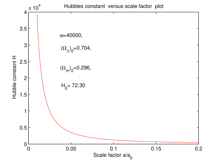
Figure 5: Variation of Hubble’s constant over scale factor

7 Certain physical properties of the universe

7.1 Matter and dark energy densities

The matter and dark energy densities of the universe are related to the energy parameters through following equation

$$\Omega_{m}=\frac{(\rho)_{m}}{\rho_{c}},\Omega_{\Lambda}=\frac{\rho_{\Lambda}}{\rho_{c}}$$ (37)

Where

$$\rho_{c}=\frac{3c^{2}H^{2}}{8\pi G}=\frac{3c^{2}\phi H^{2}}{8\pi}$$ (38)

So,

$$(\rho_{m})_{0}=(\rho_{c})_{0}(\Omega_{m})_{0}=,\;(\rho_{\Lambda})_{0}=(\rho_{c})_{0}(\Omega_{\Lambda})_{0}$$ (39)

Now

$$(\rho_{c})_{0}=\frac{3c^{2}H_{0}^{2}}{8\pi G}=1.88\;h^{2}_{0}\times 10^{-29}\;gm/cm^{3}$$

Therefore, the present value of matter and dark energy densities are given by

$$(\rho_{m})_{0}=0.5565h^{2}_{0}\times 10^{-29}gm/cm^{3}.$$ (40)

And

$$(\rho_{\Lambda})_{0}=\rho_{c}(\Omega_{\Lambda})_{0}=1.3235h^{2}_{0}\times 10^{-29}gm/cm^{3}.$$ (41)

Where we have taken

$$(\Omega_{m})_{0}=0.296\;\&\;(\Omega_{m})_{0}=0.704$$

General expressions for matter and dark energies are given by

$$\rho=(\rho)_{0}\left(\dfrac{a_{0}}{a}\right)^{3}=(\rho)_{0}\left(1+z\right)^{3}$$ (42)

And

$$(\rho_{\Lambda})=\rho_{c}\;\Omega_{\Lambda}.$$ (43)

We see that the current matter and dark energy densities are very close to the values predicted by the various surveys described in the introduction.

7.2 Age of the universe

We begin with the integral

$$t=\intop_{0}^{t}dt=\intop_{0}^{a}\frac{da}{aH}$$

$$t=\intop_{0}^{a}\frac{\sqrt{1+\frac{5\omega+6}{6(\omega+1)^{2}}}da}{aH_{0}\sqrt{(\Omega_{m})_{0}(\frac{a_{0}}{a})^{\frac{3\omega+4}{\omega+1}}+(\Omega_{\Lambda})_{0}}}$$ (44)

Integrating Eq.(44), we get the following expression for age of the universe.

$$H_{0}t=\frac{2\sqrt{1+\frac{5\omega+6}{6(\omega+1)^{2}}}}{\frac{3\omega+4}{\omega+1}\sqrt{(\Omega_{\Lambda})_{0}}}log\left(\sqrt{\frac{(\Omega_{\Lambda})_{0}}{(\Omega_{m})_{0}}\left(\frac{a}{a_{0}}\right)^{\frac{3\omega+4}{\omega+1}}}+\sqrt{1+\frac{(\Omega_{\Lambda})_{0}}{(\Omega_{m})_{0}}\left(\frac{a}{a_{0}}\right)^{\frac{3\omega+4}{\omega+1}}}\right)$$ (45)

In term of red shift, the age is given as,

$$H_{0}t=\frac{2\sqrt{1+\frac{5\omega+6}{6(\omega+1)^{2}}}}{\frac{3\omega+4}{\omega+1}\sqrt{(\Omega_{\Lambda})_{0}}}log\left(\sqrt{\frac{(\Omega_{\Lambda})_{0}}{(\Omega_{m})_{0}}\left(\frac{1}{1+z}\right)^{\frac{3\omega+4}{\omega+1}}}+\sqrt{1+\frac{(\Omega_{\Lambda})_{0}}{(\Omega_{m})_{0}}\left(\frac{1}{1+z}\right)^{\frac{3\omega+4}{\omega+1}}}\right)$$ (46)

The present age of the universe is given by

$$H_{0}t_{0}=\frac{2\sqrt{1+\frac{5\omega+6}{6(\omega+1)^{2}}}}{\frac{3\omega+4}{\omega+1}\sqrt{(\Omega_{\Lambda})_{0}}}log\left(\sqrt{\frac{(\Omega_{\Lambda})_{0}}{(\Omega_{m})_{0}}}+\sqrt{1+\frac{(\Omega_{\Lambda})_{0}}{(\Omega_{m})_{0}}}\right)$$ (47)

For $\omega=40000$, $(\Omega_{\Lambda})_{0}$=$0.704$ and $(\Omega_{m})_{0}=0.296$, $H_{0}t_{0}=0.9677$ . Since $H_{0}^{-1}=9.776h^{-}1$ Gyr = 13.5778 Gyr when $h=0.723$. Therefore $t_{0}$ = $13.0847$ Gyr. This is consistence with most recent WMAP data $t_{0}=13.73_{-0.17}^{+0.13}$ .
In Figures $6$ and $7$, we have shown the variation of time over scale factor and red shift. This also indicated the consistency with recent observations.

Figure 6: Variation of red shift over time

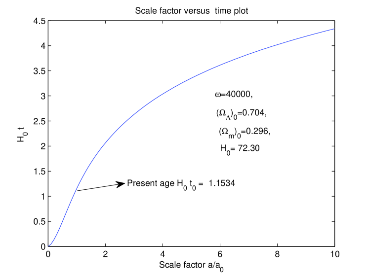
Figure 7: Variation of scale factor over time

7.3 Deceleration parameter

Eqs.(14), (20) and (23) give

$$q=\frac{\omega+2}{2(\omega+1)}-\frac{3(\omega+1)}{2\omega+3}\;\Omega_{\Lambda}$$ (48)

Using Eqs.(26) and (27), we get following expression for deceleration parameter

$$q=\frac{\omega+2}{2(\omega+1)}-\frac{3(\omega+1)}{2\omega+3}\;\left(\Omega_{\Lambda}\right)_{0}\frac{\left(1+\frac{5\omega+6}{6(\omega+1)^{2}}\right)}{\left((\Omega_{m})_{0}\left(\frac{a_{0}}{a}\right)^{\frac{3\omega+4}{\omega+1}}+(\Omega_{\Lambda})_{0}\right)}$$ (49)

In term of redshift it is given by

$$q=\frac{\omega+2}{2(\omega+1)}-\frac{3(\omega+1)}{2\omega+3}\;\left(\Omega_{\Lambda}\right)_{0}\frac{\left(1+\frac{5\omega+6}{6(\omega+1)^{2}}\right)}{\left((\Omega_{m})_{0}\left(1+z\right)^{\frac{3\omega+4}{\omega+1}}+(\Omega_{\Lambda})_{0}\right)}$$ (50)

As the present phase ($z=0$) of the universe is accelerating $q\leq 0\;ie\;\frac{\ddot{a}}{a}\geq 0$ , so we must have

$$(\Omega_{\Lambda})_{0}\geq\dfrac{(2\omega+3)(\omega+2)}{6(\omega+1)^{2}}$$ (51)

For $\omega=40000$, the limit is as follows

$$(\Omega_{\Lambda})_{0}\geq 0.3333$$

which is consistent with the present observed value of $(\Omega_{\Lambda})_{0}=0.704$. Putting $\omega=40000$, $(\Omega_{\Lambda})_{0}$=$0.704$, $(\Omega_{m})_{0}=0.296$ and $z=0$ in Eq.(50), we get the present value of deceleration parameter as

$$q_{0}=-0.5560$$ (52)

The universe attains to the accelerating phase when $z<z_{c}$ where $z=z_{c}\;at\;q=0$ . The Eq.(50) provides

$$z_{c}\cong 0.6818$$ (53)

Thus, the acceleration must have begun in the past at $z_{c}=0.6818\thicksim.5180H^{-1}_{0}yrs\thicksim 7.2371\times 10^{9}yrs$ before from present. We have converted red shift by time from Eq.(46). The figure (8) Shows how deceleration parameter increases from negative to positive over redw shift which means that in the past universe was decelerating, then at a instant $z_{c}\cong 0.6797$ it became stationary there after it starts accelerating.

Figure 8: Variation of decelerating parameter over red shift. It represents accelerating universe at present.

8 Conclusion

We summarize our results by presenting Table-2 which displays the values of cosmological parameters at present obtained by us.

Table 2: Cosmological parameters at present

Cosmological Parameters	Values at Present
BD coupling constant $\omega$	40000
$\left(\frac{\dot{G}}{G}\right)_{0}$	2.5$\times 10^{-15}$
Dark energy parameter $(\Omega_{\Lambda})_{0}$	0.704
Dust energy parameter $(\Omega_{m})_{0}$	0.296
Hubble’s constant $H_{0}$	72.30
Deceleration parameter $(q)_{0}$	-0.5560
Dust energy density $(\rho_{m})_{0}$	$0.5565h^{2}_{0}\times 10^{-29}gm/cm^{3}$
Dark energy density $(\rho_{\Lambda})_{0}$	$1.3235h^{2}_{0}\times 10^{-29}gm/cm^{3}$
Age of the universe $t_{0}$	$13.0847Gyr$

We have found that the acceleration would have begun in the past at $z_{c}=0.6818\thicksim 7.2371\times 10^{9}yrs$ before from present. These results are in good agreements with the various surveys described in the introduction.

References

- [2004] Abazajian K. et al. [SDSS Collaboration], 2004, Astron. J. 128 502.
- [2013 ] Ade P.A.R. et al., 2013, arXiv preprint astro-ph.CO/ 1303.5076 v3.
- [2016] Ade P.A.R. et al. [Planck Collaboration],2016, Planck 2015 results. XIII. Astronomy and Astrophysics, DOI: 10.1051/0004-6361/201526914, arXiv preprint astro-ph.CO/1502.01589.
- [2014] Anderson L. et al. [BOSSCollaboration], 2014, Mon. Not. R. Astron. Soc. 441 24.
- [1997] Arbab A.I., 1997, Gen. Rel. , Grav. 29, 61 .
- [2015] Aubourg E. et al. (BOSS Collaboration),2015, Physical Review, D 92 123516.
- [1995] Azar E.A. and Riazi N.,1995, Astrophys. Space Sci., 226, 1–5 .
- [2003] Azad, A, K. and Islam, J, N., Pramana, 2003, 60, 21–27 .
- [2003] Bennett C.L. et al. [WMAP Collaboration], 2003 Astrophys. J. Suppl. 148 1.
- [2003] Bertotti, B., et al., 2003, Nature, 425, 374.
- [2012] Blake C. et al. [The WiggleZ Dark Energy Survey], 2012, Mon. Not. R. Astron. Soc. 425 405.
- [1961] Brans C. and Dicke R.H., Phys. Rev., 1961, 124, 925 .
- [1998] Caldwell R.R., Dave R. and Steinhardt P.J. , 1998, Phys. Rev. Lett. 80, 1582 .
- [2002] Caldwell R.Rl, 2002, Phys. Lett. 545, 23 .
- [1992] Carvalho J.C., Lima J.A.S. and Waga I, Phys. Rev. D, 1992, 46, 2404 .
- [2000] Chiba T., Okabe T. and Yamaguchi M, 2000, Phys. Rev. D 62, 023511 .
- [2007] Copeland E.J., Sami M., Tsujikawa S., 2007 Int. J. Mod. Phys. D 15 1753.
- [2015] Delubac T. et al. [BOSS Collaboration], 2015, Astron. Astrophys. 574, A59.
- [2006] Dutta Choudhury S.B. and Sil A., 2006, Astrophys. Space Sci. 301, 61 .
- [1997] Etoh T., Hashimoto M, Arai K. and Fujimoto S., 1997, Astron. and Astrophys., 325, 893 .
- [2006] Felice, A.D. et al., 2006, Phys. Rev. D, 74, 103005
- [2015] Goswami G.K. et al ,2015, Int. J. Theo. Phys.,52, 8.
- [2016] Goswami G.K. et al ,2016, Astrophys. Space Sci.,361, 47.
- [2016] Goswami et al ,2016, Astrophys. Space Sci., 361, 119
- [2007] Gron O., and Hervik S., 2007, Einstien’s General Theory of Relativity With Modern Application in Cosmology, (New York: Springer) .
- [2013] Hrycyna O. and Lowski M.S., Phys. Rev. D., 2013, 88, 064018
- [2001] Kamenshchik A.Y., Moschella U. and Pasquier V., 2001, Phys. Lett. B 511, 265 .
- [2012] Moresco M. et al., 2012, JCAP 1208 , 006, arXiv:1201.3609.
- [2015] Moresco M., 2015, Mon. Not. R. Astron. Soc. 450 L16.
- [2002] Narlikar J.V., 2002, An Introduction to Cosmology, (Cambridge University Press) page483
- [2001] Padmanabhan T., 2001, Preprint, gr-qc/0112068.
- [1997] Perlmutter.S et al. [Supernova Cosmology Project Collaboration], 1997, Bull. Am. Astron. Soc. 29 1351.
- [1985] Pimentel L.O., 1985, Astrophys. Space Sci., 112, 175–183 .
- [2005] Qiang Li-e, Yong-ge Ma, Mu-xin Han and Dan Yu, 2005, Phys. Rev. D, 71, 061501 .
- [2002] Reyes L.M. and AguilarJ. E. M., 2002, arxiv:0902.4736 [gr-qc]
- [1998] Riess A. G. et al. [Supernova Search Team Collaboration], 1998, Astron. J. 116 1009.
- [2014] Sahni V., Shafieloo A., Starobinsky A.A.,2014, Astrophys. J. 793 L40.
- [2000] Sahni V. and Starobinsky A.A., 2000, Int. J. Mod. Phys. D 9 373.
- [2004] Shapiro I.L. and Sola J., 2004, Preprint, astroph/ 0401015 .
- [1984] Singh T. and Singh T., J. Math. Phys., 1984, 25, 9 .
- [2011] Smolyakov M.A., 2011, arxiv:0711.3811vz [gr-qc]
- [2003] Spergel D.N. et al. [WMAP Collaboration], 2003, Astrophys. J. Suppl. 148 175.
- [2010] Stern D., Jimenez R., Verde L., Kamionkowski M., Stanford S. A., 2010, JCAP 1002 008.
- [2012] Suzuki,N. et al.,2012, Astrophysical Journal, 746 85.
- [2004] Tegmark M. et al. [SDSS Collaboration], 2004 Phys. Rev. D 69 103501.
- [2002] Vishwakarma R.G., 2002, Class. Quant. Grav. 19, 4747 .
- [1995] Wetterich C., Astron. Astrophys., 1995, 301, 321 .
- [2012] Yadav, A.K. et al.,2012, Eur. Phys. J. Plus 127: 127.
- [2014] Zhang C., Zhang H., Yuan S., Zhang T.J., Sun Y.C., 2014, Astron. Astrophys. 14 1221.