Multilevel ensemble Kalman filtering for spatio-temporal processes

Alexey Chernov HÅkon Hoel Kody J. H. Law Fabio Nobile§  and  Raul Tempone
Abstract.

We design and analyse the performance of a multilevel ensemble Kalman filter method (MLEnKF) for filtering settings where the underlying state-space model is an infinite-dimensional spatio-temporal process. We consider underlying models that needs to be simulated by numerical methods, with discretization in both space and time. The multilevel Monte Carlo (MLMC) sampling strategy, achieving variance reduction through pairwise coupling of ensemble particles on neighboring resolutions, is used in the sample-moment step of MLEnKF to produce an efficient hierarchical filtering method for spatio-temporal models. Under sufficient regularity, MLEnKF is proven to be more efficient for weak approximations than EnKF, asymptotically in the large-ensemble and fine-numerical-resolution limit. Numerical examples support our theoretical findings.


Key words: Monte Carlo, multilevel, filtering, ensemble Kalman filter, stochastic partial differential equations (SPDE).


AMS subject classification: 65C30, 65Y20

Institute for Mathematics, Carl von Ossietzky University Oldenburg, Germany (alexey.chernov@uni-oldenburg.de)
Chair of Mathematics for Uncertainty Quantification, RWTH Aachen University, Aachen, Germany (hoel@uq.rwth-aachen.de)
School of Mathematics, University of Manchester, United Kingdom (kody.law@manchester.ac.uk)
§ Mathematics Institute of Computational Science and Engineering, École polytechnique fédérale de Lausanne, Switzerland (fabio.nobile@epfl.ch)
Chair of Mathematics for Uncertainty Quantification, RWTH Aachen University, Aachen, Germany (tempone@uq.rwth-aachen.de) and Applied Mathematics and Computational Sciences, KAUST, Thuwal, Saudi Arabia.

1. Introduction

Filtering refers to the sequential estimation of the state $u$ and/or parameters of a system through sequential incorporation of online data $y$. The most complete estimation of the state $u_{n}$ at time $n$ is given by its probability distribution conditional on the observations up to the given time $\mathbb{P}(du_{n}|y_{1},\ldots,y_{n})$ [27, 2]. For linear Gaussian systems, the analytical solution may be given in closed form via update formulae for the mean and covariance known as the Kalman filter [31]. More generally, however, closed form solutions typically are not known. One must therefore resort to either algorithms which approximate the probabilistic solution by leveraging ideas from control theory in the data assimilation community [32, 27], or Monte Carlo methods to approximate the filtering distribution itself [2, 15, 11]. The ensemble Kalman filter (EnKF) [9, 17, 35] combines elements of both approaches. In the linear Gaussian case it converges to the Kalman filter solution in the large-ensemble limit [41], and even in the nonlinear case, under suitable assumptions it converges [37, 36] to a limit which is optimal among those which incorporate the data linearly and use a single update iteration [36, 40, 44]. In the case of spatially extended models approximated on a numerical grid, the state space itself may become very high-dimensional and even the linear solves may become intractable, due to the cost of computing the covariance matrix. Therefore, one may be inclined to use the EnKF filter even for linear Gaussian problems in which the solution is computationally intractable despite being given in closed form by the Kalman filter.

The Multilevel Monte Carlo method (MLMC) is a hierarchical and variance-reduction based approximation method initially developed for weak approximations of random fields and stochastic differential equations [21, 18, 19]. Recently, a number of works have emerged which extend the MLMC framework to the setting of Monte Carlo algorithms designed for Bayesian inference. Examples include Markov chain Monte Carlo [14, 22], sequential Monte Carlo samplers [6, 26, 42], particle filters [25, 20], and EnKF [23]. The filtering papers thus far [25, 20, 23] consider only finite-dimensional SDE forward models. In this work, we develop a new multilevel ensemble Kalman filtering method (MLEnKF) for the setting of infinite-dimensional state-space models with evolution in continuous-time. The method consists of a hierarchy of pairwise coupled EnKF-like ensembles on different finite-resolution levels of the underlying infinite-dimensional evolution model that all depend on the same Kalman gain in the update step. The method presented in this work may be viewed as an extension of the finite-dimensional-state-space MLEnKF method [23], which only considered a hierarchy of time-discretization resolution levels.

Under sufficient regularity, the large-ensemble limit of EnKF is equal in distribution to the so-called mean-field EnKF (MFEnKF), cf. [37, 36, 34]. In nonlinear settings, however, MFEnKF is not equal in distribution to the Bayes filter, which is the exact filter distribution. More precisely, the error of EnKF approximating the Bayes filter may be decomposed into a statistical error, due to the finite ensemble size, and a Gaussian bias that is introduced by the Kalman-filter-like update step in EnKF. While the update-step bias error in EnKF is difficult both to quantify and deal with, the statistical error can, in theory, be reduced to arbitrary magnitude. However, the high computational cost of simulations in high-dimensional state space often imposes small ensemble size as a practical constraint. By making use of hierarchical variance-reduction techniques, the MLEnKF method developed in this work is capable of obtaining a much smaller statistical error than EnKF at the same fixed cost.

In addition to design an MLEnKF method for spatio-temporal processes, we provide an asymptotic performance analysis of the method that is applicable under sufficient regularity of the filtering problem and $L^{p}$-strong convergence of the numerical method approximating the underlying model dynamics. Sections 5 and 6 are devoted to a detailed analysis and practical implementation of MLEnKF applied to linear and semilinear stochastic reaction-diffusion equations. In particular, we describe how the pairwise coupling of EnKF-like hierarchies should be implemented for one specific numerical solver (the exponential-Euler method), and provide numerical evidence for the efficiency gains of MLEnKF over EnKF.

Since particle filters are known to often perform better than EnKF, we also include a few remarks on how we believe such methods would compare to MLEnKF in filtering settings with spatial processes. Due to the poor scaling of particle ensemble size in high dimensions, which can even be exponential [7, 38], particle filters are typically not used for spatial processes, or even modestly high-dimensional processes. There has been some work in the past few years which overcomes this issue either for particular examples [5] or by allowing for some bias [4, 48, 45, 49]. But particle filters cannot yet be considered practically applicable for general spatial processes. If there is a well-defined limit of the model as the state-space dimension $d$ grows such that the effective dimension of the target density with respect to the proposal remains finite or even small, then useful particle filters can be developed [33, 39]. As noted in [10], the key criterion which needs to be satisfied is that the proposal and the target are not mutually singular in the limit. MLMC has been applied recently to particle filters, in the context where the approximation arises due to time discretization of a finite-dimensional SDE [25, 20]. It is an interesting open problem to design multilevel particle filters for spatial processes: Both the range of applicability and the asymptotic performance of such a method versus MLEnKF when applied to spatial processes are topics that remain to be studied.

The rest of the paper is organized as follows. Section 2 introduces the filtering problem and notation. The design of the MLEnKF method is presented in section 3. Section 4 studies the weak approximation of MFEnKF by MLEnKF, and shows that in this setting, MLEnKF inherits almost the same favorable asymptotic “cost-to-accuracy” performance as standard MLMC applied to weak approximations of stochastic spatio-temporal processes. Section5 presents a detailed analysis and description of the implementation of MLEnKF for a family of stochastic reaction-diffusion models. Section 6 provides numerical studies of filtering problems with linear and semilinear stochastic reaction-diffusion models that corroborate our theoretical findings. Conclusions and future directions are presented in section 7, and auxiliary theoretical results and technical proofs are provided in Appendices AB and C.

2. Set-up and single level algorithm

2.1. General set-up

Let $(\Omega,\mathcal{F},\mathbb{P})$ be a complete probability space, where $\mathbb{P}$ is a probability measure on the measurable space $(\Omega,\mathcal{F})$. Let $\mathcal{V}$ be a separable Hilbert space with inner product $\langle\cdot,\cdot\rangle_{\mathcal{V}}$ and norm $\|\cdot\|_{\mathcal{V}}=\sqrt{\langle\cdot,\cdot\rangle_{\mathcal{V}}}$. Let $V$ denote a subspace of $\mathcal{V}$ which is closed in the topology induced by the norm $\|\cdot\|_{V}=\sqrt{\langle\cdot,\cdot\rangle_{V}}$, which is assumed to be a stronger norm than $\|\cdot\|_{\mathcal{V}}$. For an arbitrary separable Hilbert space $(\mathcal{K},\|\cdot\|_{\mathcal{K}})$, we denote the associated $L^{p}$-Bochner space by

$$L^{p}(\Omega,\mathcal{K})=\{u:\Omega\rightarrow\mathcal{K}\mid u\text{ is measurable and }\mathbb{E}\mspace{-2.0mu}\left[\|u\|^{p}_{\mathcal{K}}\right]<\infty\},\quad\text{for }p\in[1,\infty),$$

where $\|u\|_{L^{p}(\Omega,\mathcal{K})}=(\mathbb{E}\mspace{-2.0mu}\left[\|u\|^{p}_{\mathcal{K}}\right])^{1/p}$, or the shorthand $\|u\|_{p}$ whenever confusion is not possible. For an arbitrary pair of Hilbert spaces $\mathcal{K}_{1}$ and $\mathcal{K}_{2}$, the space of bounded linear mappings from the former space into the latter is denoted by

$$L(\mathcal{K}_{1},\mathcal{K}_{2})\mathrel{\mathop{:}}=\left\{H:\mathcal{K}_{1}\to\mathcal{K}_{2}\mid H\text{ is linear and }\|H\|_{L(\mathcal{K}_{1},\mathcal{K}_{2})}<\infty\right\},$$

where

$$\|H\|_{L(\mathcal{K}_{1},\mathcal{K}_{2})}\mathrel{\mathop{:}}=\sup_{x\in\mathcal{K}_{1}\setminus\{0\}}\frac{\|Hx\|_{\mathcal{K}_{2}}}{\|x\|_{\mathcal{K}_{1}}}.$$

In finite dimensions, $(\mathbb{R}^{m},\langle\cdot,\cdot\rangle)$ represents the $m$-dimensional Euclidean vector space with norm $|\cdot|\mathrel{\mathop{:}}=\sqrt{\langle\cdot,\cdot\rangle}$, and for matrices $A\in L(\mathbb{R}^{m_{1}},\mathbb{R}^{m_{2}})$, $|A|:=\|A\|_{L(\mathbb{R}^{m_{1}},\mathbb{R}^{m_{2}})}$.

2.1.1. The filtering problem

Given $u_{0}\in\cap_{p\geq 2}L^{p}(\Omega,V)$ and the mapping $\Psi:L^{p}(\Omega,V)\times\Omega\rightarrow L^{p}(\Omega,V)$, we consider the discrete-time dynamics

$$u_{n+1}(\omega)=\Psi(u_{n},\omega),\quad\text{for}\quad n=0,1,\ldots,N-1.$$ (1)

and the sequence of observations

$$y_{n}(\omega)=Hu_{n}(\omega)+\eta_{n}(\omega),\quad n=1,2,\ldots,N.$$ (2)

Here, $H\in L(\mathcal{V},\mathbb{R}^{m})$, the sequence $\{\eta_{n}\}$ consists of independent and identically $N(0,\Gamma)-$distributed random variables with $\Gamma\in\mathbb{R}^{m\times m}$ positive definite. In the sequel, the explicit dependence on $\omega$ will be suppressed where confusion is not possible. A general filtering objective is to track the signal $u_{n}$ given a fixed sequence of observations $Y_{n}:=(y_{1},y_{2},\ldots,y_{n})$, i.e., to track the distribution of $u_{n}|Y_{n}$ for $n=1,\ldots$. In this work, however, we restrict ourselves to considering the more specific objective of approximating $\mathbb{E}\mspace{-2.0mu}\left[\varphi(u_{n})|Y_{n}\right]$ for a given quantity of interest (QoI) $\varphi:\mathcal{V}\to\mathbb{R}$. The index $n$ will be referred to as time, whether the actual time between observations is 1 or not (in the examples in Section5 and beyond it will be called $T$), but this will not cause confusion since time is relative.

2.1.2. The dynamics

We consider problems in which $\Psi$ is the finite-time evolution of an SPDE, e.g. (35), and we will assume that $\Psi$ cannot be evaluated exactly, but that there exists a sequence $\{\Psi^{\ell}:L^{p}(\Omega,\mathcal{V})\times\Omega\to L^{p}(\Omega,\mathcal{V})\}_{\ell=0}^{\infty}$ of approximations to the solution $\Psi:=\Psi^{\infty}$ satisfying the following uniform-in-$\ell$ stability properties

Assumption 1.

For every $p\geq 2$, it holds that $\Psi:L^{p}(\Omega,V)\times\Omega\to L^{p}(\Omega,V)$, and for all $u,v\in L^{p}(\Omega,\mathcal{V})$, the solution operators $\{\Psi^{\ell}\}_{\ell=0}^{\infty}$ satisfy the following conditions: there exists a constant $0<c_{\Psi}<\infty$ depending on $p$ such that

  • (i)

    $\|\Psi^{\ell}(u)-\Psi^{\ell}(v)\|_{L^{p}(\Omega,\mathcal{V})}{\leq}c_{\Psi}\|u-v\|_{L^{p}(\Omega,\mathcal{V})}$ , and

  • (ii)

    $\|\Psi^{\ell}(u)\|_{L^{p}(\Omega,\mathcal{V})}\leq c_{\Psi}(1+\|u\|_{L^{p}(\Omega,\mathcal{V})})$.

For notational simplicity, we restrict ourselves to settings in which the map $\Psi(\cdot)$ does not depend on $n$, but the results in this work do of course extend easily to non-autonomous settings when the assumptions on $\{\Psi_{n}\}_{n=1}^{N}$ are uniform with respect to $n$.

Remark 1.

The two approximation spaces $V\subset\mathcal{V}$ are introduced in order to obtain convergence rates for numerical simulation methods $\Psi^{\ell}$ that are discretized in physical or state space. See Assumption 2(i)-(ii) and inequality (41) for an example of how this may be obtained in practice.

2.1.3. The Bayes filter

The pair of discrete-time stochastic processes $(u_{n},y_{n})$ constitutes a hidden Markov model, and the exact (Bayes-filter) distribution of $u_{n}|Y_{n}$ may in theory be determined iteratively through the system of prediction-update equations

$\displaystyle\mathbb{P}(du_{n}|Y_{n})$ $\displaystyle=\frac{1}{Z(Y_{n})}{\mathcal{L}(u_{n};y_{n})\mathbb{P}(du_{n}|Y_{n-1})},$
$\displaystyle\mathbb{P}(du_{n}|Y_{n-1})$ $\displaystyle=\int_{u_{n-1}\in\mathcal{V}}\mathbb{P}(du_{n}|u_{n-1})\mathbb{P}(du_{n-1}|Y_{n-1}),$
$\displaystyle\mathcal{L}(u_{n};y_{n})$ $\displaystyle=\exp\Big{\{}-\frac{1}{2}|\Gamma^{-1/2}(y_{n}-Hu_{n})|^{2}\Big{\}},$
$\displaystyle Z(Y_{n})$ $\displaystyle=\int_{u_{n}\in\mathcal{V}}\mathcal{L}(u_{n};y_{n})\mathbb{P}(du_{n}|Y_{n-1}).$

When the state space is infinite-dimensional and the dynamics cannot be evaluated exactly, however, this is an extremely challenging problem. Consequently, we will here restrict ourselves to constructing weak approximation methods of the mean-field EnKF, cf. Section 2.4.

2.2. Some details on Hilbert spaces, Hilbert-Schmidt operators, and Cameron-Martin spaces

For two arbitrary separable Hilbert spaces $\mathcal{K}_{1}$ and $\mathcal{K}_{2}$, the tensor product $\mathcal{K}_{1}\otimes\mathcal{K}_{2}$ is also a Hilbert space. For rank-1 tensors, its inner product is defined by

$$\langle u\otimes v,u^{\prime}\otimes v^{\prime}\rangle_{\mathcal{K}_{1}\otimes\mathcal{K}_{2}}=\langle u,u^{\prime}\rangle_{\mathcal{K}_{1}}\langle v,v^{\prime}\rangle_{\mathcal{K}_{2}}\qquad\forall u,u^{\prime}\in\mathcal{K}_{1},\quad\forall v,v^{\prime}\in\mathcal{K}_{2},$$

which extends by linearity to any tensor of finite rank. The Hilbert space $\mathcal{K}_{1}\otimes\mathcal{K}_{2}$ is the completion of this set with respect to the induced norm

$$\|u\otimes v\|_{\mathcal{K}_{1}\otimes\mathcal{K}_{2}}=\|u\|_{\mathcal{K}_{1}}\|v\|_{\mathcal{K}_{2}}.$$ (3)

Let $\{e_{k}\}$ and $\{\hat{e}_{k}\}$ be orthonormal bases for $\mathcal{K}_{1}$ and $\mathcal{K}_{2}$, respectively, and observe that finite sums of rank-1 tensors of the form $X\mathrel{\mathop{:}}=\sum_{i,j}\alpha_{ij}e_{i}\otimes\hat{e}_{j}\in\mathcal{K}_{1}\otimes\mathcal{K}_{2}$ can be identified with a bounded linear mapping

$$T_{X}:\mathcal{K}_{2}^{*}\to\mathcal{K}_{1}\quad\text{with}\quad T_{X}(f)\mathrel{\mathop{:}}=\sum_{i,j}\alpha_{ij}f(\hat{e}_{j})e_{i},\quad\text{for }f\in\mathcal{K}_{2}^{*}.$$ (4)

For two bounded linear operators $A,B:\mathcal{K}_{2}^{*}\to\mathcal{K}_{1}$ we recall the definition of the Hilbert-Schmidt inner product and norm

$$\langle A,B\rangle_{HS}=\sum_{k}\langle A\hat{e}^{*}_{k},B\hat{e}^{*}_{k}\rangle_{\mathcal{K}_{1}},\qquad|A|_{HS}=\langle A,A\rangle_{HS}^{1/2},$$

where $\{\hat{e}^{*}_{k}\}$ is the orthonormal basis of $\mathcal{K}_{2}^{*}$ satisfying $\hat{e}^{*}_{k}(\hat{e}_{j})=\delta_{jk}$ for all $j,k$ in the considered index set. A bounded linear operator $A:\mathcal{K}_{2}^{*}\to\mathcal{K}_{1}$ is called a Hilbert-Schmidt operator if $|A|_{HS}<\infty$ and $HS(\mathcal{K}_{2}^{*},\mathcal{K}_{1})$ is the space of all such operators. In view of (4),

$$\begin{split}|T_{X}|_{HS}^{2}&=\sum_{k}\left\langle\sum_{i,j}\alpha_{ij}e^{*}_{k}(\hat{e}_{j})e_{i},\sum_{i^{\prime},j^{\prime}}\alpha_{i^{\prime}j^{\prime}}e^{*}_{k}(\hat{e}_{j^{\prime}})e_{i^{\prime}}\right\rangle_{\mathcal{K}_{1}}\\ &=\sum_{i,j}|\alpha_{ij}|^{2}\\ &=\|X\|_{\mathcal{K}_{1}\otimes\mathcal{K}_{2}}.\end{split}$$

By completion, the space $\mathcal{K}_{1}\otimes\mathcal{K}_{2}$ is isometrically isomorphic to $HS(\mathcal{K}_{2}^{*},\mathcal{K}_{1})$ (and also to $HS(\mathcal{K}_{2},\mathcal{K}_{1})$ by the Riesz representation theorem). For an element $A\in\mathcal{K}_{1}\otimes\mathcal{K}_{2}$ we identify the norms

$$\|A\|_{\mathcal{K}_{1}\otimes\mathcal{K}_{2}}=|A|_{HS},$$

and such elements will interchangeably be considered either as members of $\mathcal{K}_{1}\otimes\mathcal{K}_{2}$ or of $HS(\mathcal{K}_{2}^{*},\mathcal{K}_{1})$. When viewed as $A\in HS(\mathcal{K}_{2}^{*},\mathcal{K}_{1})$, the mapping $A:\mathcal{K}_{2}^{*}\to\mathcal{K}_{1}$ is defined by

$$Af\mathrel{\mathop{:}}=\sum_{i,j}A_{ij}f(\hat{e}_{j})e_{i},\quad\text{for }f\in\mathcal{K}_{2}^{*},$$

where $A_{ij}\mathrel{\mathop{:}}=\langle e_{i},A\hat{e}_{j}^{*}\rangle_{\mathcal{K}_{1}}$, and when viewed as $A\in\mathcal{K}_{1}\otimes\mathcal{K}_{2}$, we use tensor-basis representation

$$A=\sum_{i,j}A_{ij}e_{i}\otimes\hat{e}_{j}.$$

The covariance operator for a pair of random variables $Z,X\in L^{2}(\Omega,V)$ is denoted by

$$\mathrm{Cov}[Z,X]\mathrel{\mathop{:}}=\mathbb{E}\mspace{-2.0mu}\left[(Z-\mathbb{E}\mspace{-2.0mu}\left[Z\right])\otimes(X-\mathbb{E}\mspace{-2.0mu}\left[X\right])\right]\in V\otimes V,$$

and whenever $Z=X$, we employ the shorthand $\mathrm{Cov}[Z]\mathrel{\mathop{:}}=\mathrm{Cov}[Z,Z]$. For completeness and later reference, let us prove that said covariance belongs to $V\otimes V$.

Proposition 1.

If $u\in L^{2}(\Omega,V)$, then $C:=\mathrm{Cov}[u]\in V\otimes V$.

Proof.

By Jensen’s inequality,

$$\begin{split}\|C\|_{V\otimes V}&=\|\mathbb{E}\mspace{-2.0mu}\left[(u-\mathbb{E}\mspace{-2.0mu}\left[u\right])\otimes(u-\mathbb{E}\mspace{-2.0mu}\left[u\right])\right]\|_{V\otimes V}\\ &\leq\mathbb{E}\mspace{-2.0mu}\left[\left\|(u-\mathbb{E}\mspace{-2.0mu}\left[u\right])\otimes(u-\mathbb{E}\mspace{-2.0mu}\left[u\right])\right\|_{V\otimes V}\right]\\ &=\left\|u-\mathbb{E}\mspace{-2.0mu}\left[u\right]\right\|_{L^{2}(\Omega,V)}^{2}\\ &=\|u\|_{L^{2}(\Omega,V)}^{2}-\left\|\mathbb{E}\mspace{-2.0mu}\left[u\right]\right\|_{V}^{2}<\infty.\end{split}$$

2.3. Ensemble Kalman filtering

EnKF is an ensemble-based extension of Kalman filtering to nonlinear settings. Let $\{\hat{v}_{0,i}\}_{i=1}^{M}$ denote an ensemble of $M$ i.i.d. particles with $\hat{v}_{0,i}\stackrel{{\scriptstyle D}}{{=}}u_{0}$. The initial distribution $\mathbb{P}_{u_{0}}$ can thus be approximated by the empirical measure of $\{\hat{v}_{0,i}\}_{i=1}^{M}$. By extension, let $\{\hat{v}_{n,i}\}_{i=1}^{M}$ denote the ensemble-based approximation of the updated distribution $u_{n}|Y_{n}$ (at $n=0$ we employ the convention $Y_{0}=\emptyset$, so that $u_{0}=u_{0}|Y_{0}$). Given an updated ensemble $\{\hat{v}_{n,i}\}_{i=1}^{M}$, the ensemble-based approximation of the prediction distribution $u_{n+1}|Y_{n}$ is obtained through simulating each particle one observation time ahead:

$$v_{n+1,i}=\Psi(\hat{v}_{n,i}),\quad i=1,2,\ldots,M.$$ (5)

We will refer to $\{\hat{v}_{n+1,i}\}_{i=1}^{M}$ as the prediction ensemble at time $n+1$, and we also note that in many settings, the exact dynamics $\Psi$ in (5) have to be approximated by a numerical solver.

Next, given $\{\hat{v}_{n+1,i}\}_{i=1}^{M}$ and a new observation $y_{n+1}$, the ensemble-based approximation of the updated distribution $u_{n+1}|Y_{n+1}$ is obtained through updating each particle path

$$\begin{split}\tilde{y}_{n+1,i}&=y_{n+1}+\eta_{n+1,i},\\ \hat{v}_{n+1,i}&=(I-K^{\rm MC}_{n+1}H)v_{n+1,i}+K^{\rm MC}_{n+1}\tilde{y}_{n+1,i},\end{split}$$ (6)

where $\{\eta_{n+1,i}\}_{i=1}^{M}$ is an independent and identically $N(0,\Gamma)-$distributed sequence, the Kalman gain

$$K^{\rm MC}_{n+1}=\left(C_{n+1}^{\rm MC}H^{*}\right)(S^{\rm MC}_{n+1})^{-1}$$

is a function of

$$S^{\rm MC}_{n+1}=HC_{n+1}^{\rm MC}H^{*}+\Gamma,$$

the adjoint observation operator $H^{*}\in L(\mathbb{R}^{m},\mathcal{V}^{*})$, defined by

$$(H^{*}a)(w)=\langle a,Hw\rangle\quad\text{for all}\quad a\in\mathbb{R}^{m}\quad\text{and}\quad w\in\mathcal{V},$$

and the prediction covariance

$$\begin{split}C_{n+1}^{\rm MC}&=\mathrm{Cov}_{M}[v_{n+1}]\ ,\end{split}$$

with

$$\mathrm{Cov}_{M}[u_{n},v_{n}]\mathrel{\mathop{:}}=\frac{M}{M-1}\left(E_{M}[u_{n}\otimes v_{n}]-E_{M}[u_{n}]\otimes E_{M}[v_{n}]\right)\,$$ (7)
$$E_{M}[v_{n}]\mathrel{\mathop{:}}=\frac{1}{M}\sum_{i=1}^{M}v_{n,i}\,$$

and the shorthand $\mathrm{Cov}_{M}[u_{n}]\mathrel{\mathop{:}}=\mathrm{Cov}_{M}[u_{n},u_{n}]$.

We introduce the following notation for the empirical measure of the updated ensemble $\{\hat{v}_{n,i}\}_{i=1}^{M}$:

$$\hat{\mu}^{\rm MC}_{n}=\frac{1}{M}\sum_{i=1}^{M}\delta_{\hat{v}_{n,i}},$$ (8)

and for any QoI $\varphi:\mathcal{V}\rightarrow\mathbb{R}$, let

$$\hat{\mu}_{n}^{\rm MC}[\varphi]:=\int\varphi d\hat{\mu}^{\rm MC}_{n}=\frac{1}{M}\sum_{i=1}^{M}\varphi(\hat{v}_{n,i}).$$

Due to the update formula (6), all ensemble particles are correlated to one another after the first update. Even in the linear Gaussian case, the ensemble will not remain Gaussian after the first update. Nonetheless, it has been shown that the in the large-ensemble limit, EnKF converges in $L^{p}(\Omega)$ to the correct (Bayes-filter) Gaussian in the linear and finite-dimensional case [41, 37], with the rate $\mathcal{O}(M^{-1/2})$ for Lipschitz-functional QoI with polynomial growth at infinity. Furthermore, in the nonlinear cases admitted by Assumption 1, EnKF converges in the same sense and with the same rate to a mean-field limiting distribution described below.

Remark 2.

The perturbed observations $\tilde{y}_{n,i}$ were originally introduced in [9] to correct the variance-deflation-type error that appeared in its absence in implementations following the original formulation of EnKF [16]. It has become known as the perturbed observation implementation.

2.4. Mean-field Ensemble Kalman Filtering

In order to describe and study convergence properties of EnKF in the large-ensemble limit, we now introduce the mean-field EnKF (MFEnKF) [36]: Let $\hat{\bar{v}}_{0}\sim\mathbb{P}_{u_{0}}$ and

$$\qquad\qquad\quad\mbox{Predict}\;\left\{\begin{array}[]{lll}\bar{v}_{n+1}&=\Psi(\hat{\bar{v}}_{n}),\\ \bar{m}_{n+1}&=\mathbb{E}\mspace{-2.0mu}\left[\bar{v}_{n+1}\right],\\ \bar{C}_{n+1}&=\mathbb{E}\mspace{-2.0mu}\left[({\bar{v}}_{n+1}-\bar{m}_{n+1})\otimes({\bar{v}}_{n+1}-\bar{m}_{n+1})\right]\end{array}\right.$$ (9)
$$\mbox{Update}\left\{\begin{array}[]{llll}\bar{S}_{n+1}&=H\bar{C}_{n+1}H^{*}+\Gamma\\ \bar{K}_{n+1}&=\bar{C}_{n+1}H^{*}\bar{S}_{n+1}^{-1}\\ {\tilde{y}}_{n+1}&=y_{n+1}+\eta_{n+1}\\ \hat{\bar{v}}_{n+1}&=(I-\bar{K}_{n+1}H){\bar{v}}_{n+1}+\bar{K}_{n+1}{\tilde{y}}_{n+1}.\\ \end{array}\right.$$ (10)

Here $\eta_{n}$ are i.i.d. draws from $N(0,\Gamma).$ In the finite-dimensional state-space setting, it was shown in [37] and [36] that for nonlinear state-space models and nonlinear models with additive Gaussian noise, respectively, EnKF converges to MFEnKF with the $L^{p}(\Omega)$ convergence rate $\mathcal{O}(M^{-1/2})$, as long as the models satisfy a Lipschitz criterion, similar to (but stronger than) Assumption 1. And in [23], we showed for that MLEnKF converges toward MFEnKF with a higher rate than EnKF does in said finite-dimensional setting. The work [34] extended convergence results to infinite-dimensional state space for square-root filters. In this work, the aim is to prove convergence of the MLEnKF for infinite-dimensional state space, with the same favorable asymptotic cost-to-accuracy performance as in [23].

The following $L^{p}$-boundedness properties ensures the existence of the MFEnKF-process and its mean-field Kalman gain, and they will be needed when studying the properteis of MLEnKF:

Proposition 2.

Assume the initial data of the hidden Markov model (1) and (2) satisfies $u_{0}\in\cap_{p\geq 2}L^{p}(\Omega,V)$. Then the MFEnKF process (9)–(10) satisfies $\bar{v}_{n},\hat{\bar{v}}_{n}\in\cap_{p\geq 2}L^{p}(\Omega,V)$ and $\|\bar{K}_{n}\|_{L(\mathbb{R}^{m},V)}<\infty$ for all $n\in\mathbb{N}$.

Proof.

Since $\hat{\bar{v}}_{0}=u_{0}$, the property clearly holds for $n=0$. Given $\hat{\bar{v}}_{n}\in L^{p}(\Omega,V)$, Assumption 1 guarantees $\bar{v}_{n+1}\in L^{p}(\Omega,V)$. By Proposition 1, $\bar{C}_{n+1}\in V\otimes V$. Since $H\bar{C}_{n+1}H^{*}\geq 0$ and $\Gamma>0$, it follows that $H^{*}\bar{S}_{n+1}^{-1}\in L(\mathbb{R}^{m},\mathcal{V}^{*})$ as

$$\begin{split}\|H^{*}\bar{S}_{n+1}^{-1}\|_{L(\mathbb{R}^{m},\mathcal{V}^{*})}&\leq\|H^{*}\|_{L(\mathbb{R}^{m},\mathcal{V}^{*})}|\bar{S}_{n+1}^{-1}|\\ &\leq\|H\|_{L(\mathcal{V},\mathbb{R}^{m})}|\Gamma^{-1}|\\ &<\infty.\end{split}$$

Furthermore, since $\mathcal{V}^{*}\subset V^{*}$ it also holds that $\|H^{*}\bar{S}_{n+1}^{-1}\|_{L(\mathbb{R}^{m},V^{*})}<\infty$ and

$$\begin{split}\|\bar{K}_{n+1}\|_{L(\mathbb{R}^{m},V)}&\leq\|\bar{C}_{n+1}\|_{L(V^{*},V)}\|H^{*}\bar{S}_{n+1}^{-1}\|_{L(\mathbb{R}^{m},V^{*})}\\ &\leq\|\bar{C}_{n+1}\|_{V\otimes V}\|H^{*}\bar{S}_{n+1}^{-1}\|_{L(\mathbb{R}^{m},V^{*})}\\ &<\infty.\end{split}$$

The result follows by recalling that $V\subset\mathcal{V}$ and by the triangle inequality:

$\displaystyle\|\hat{\bar{v}}_{n+1}\|_{L^{p}(\Omega,V)}$ $\displaystyle\leq\|\bar{v}_{n+1}\|_{L^{p}(\Omega,V)}$
$\displaystyle\quad+\|\bar{K}_{n+1}\|_{L(\mathbb{R}^{m},V)}\left(\|H\bar{v}_{n+1}\|_{L^{p}(\Omega,\mathbb{R}^{m})}+\|\tilde{y}_{n+1}\|_{L^{p}(\Omega,\mathbb{R}^{m})}\right)$
$\displaystyle<\infty.$

We conclude this section with some remarks on tensorized representations of the Kalman gain and related auxiliary operators that will be useful when developing MLEnKF algorithms in Section 3.3.

2.4.1. The Kalman gain and auxiliary operators

Introducing complete orthonormal bases $\{e_{i}\}_{i=1}^{m}$ for $\mathbb{R}^{m}$, and $\{\phi_{j}\}$ for $\mathcal{V}$, it follows that $H\in L(\mathcal{V},\mathbb{R}^{m})$ can be written

$$H=\sum_{i=1}^{m}\sum_{j=1}^{\infty}H_{ij}e_{i}\otimes\phi_{j}^{*}$$

with $H_{ij}\mathrel{\mathop{:}}=\langle e_{i},H\phi_{j}\rangle$. And since $\|H\|_{L(\mathcal{V},\mathbb{R}^{m})}<\infty$, it holds that

$$\sum_{j=1}^{\infty}H_{ij}\phi_{j}^{*}\in\mathcal{V}^{*},\quad\text{for all }i\in\{1,2,\ldots,m\}.$$

For the covariance matrix, it holds almost surely that ${C}^{\mathrm{MC}}_{n+1}\in V\otimes V\subset\mathcal{V}\otimes\mathcal{V}$, so it may be represented by

$${C}^{\mathrm{MC}}_{n+1}=\sum_{i,j=1}^{\infty}C_{n+1,ij}^{{\rm MC}}\phi_{i}\otimes\phi_{j},\quad\text{where}\quad C_{n+1,ij}^{{\rm MC}}\mathrel{\mathop{:}}=\langle\phi_{i},{C}^{\mathrm{MC}}_{n+1}\phi_{j}^{*}\rangle_{\mathcal{V}}.$$

For the auxiliary operator, it holds almost surely that

$$R^{\rm MC}_{n+1}\mathrel{\mathop{:}}=C_{n+1}^{\rm MC}H^{*}\in L(\mathbb{R}^{m},V),$$

so it can be represented by

$$R^{\rm MC}_{n+1}=\sum_{i=1}^{m}\sum_{j=1}^{\infty}R^{{\rm MC}}_{n+1,ij}\phi_{i}\otimes e_{j},\quad\text{where}\quad R^{{\rm MC}}_{n+1,ij}=\sum_{k=1}^{\infty}C_{n+1,ik}^{{\rm MC}}H_{jk}.$$

Lastly, since $(S^{\rm MC})^{-1}\in L(\mathbb{R}^{m},\mathbb{R}^{m})$ and $K^{{\rm MC}}\in L(\mathbb{R}^{m},V)$ almost surely, it holds that

$$S^{\rm MC}_{n+1,ij}=\left(\sum_{k=1}^{\infty}H_{ik}R^{{\rm MC}}_{n+1,kj}\right)+\Gamma_{ij}\text{ and }K^{{\rm MC}}_{n+1,ij}=\sum_{k=1}^{m}R^{{\rm MC}}_{n+1,ik}\left((S^{\rm MC}_{n+1})^{-1}\right)_{kj}.$$

3. Multilevel EnKF

3.1. Notation and assumptions

Recall that $\{\phi_{k}\}_{k=1}^{\infty}$ represents a complete orthonormal basis for $\mathcal{V}$ and consider the hierarchy of subspaces $\mathcal{V}_{\ell}={\rm span}\{\phi_{k}\}_{k=1}^{N_{\ell}}$, where $\{N_{\ell}\}$ is an exponentially increasing sequence of natural numbers further described below in Assumption 2. By construction, $\mathcal{V}_{0}\subset\mathcal{V}_{1}\subset\dots\subset\mathcal{V}$. We define a sequence of orthogonal projection operators $\{\mathcal{P}_{\ell}:\mathcal{V}\to\mathcal{V}_{\ell}\}$ by

$$\mathcal{P}_{\ell}v\mathrel{\mathop{:}}=\sum_{j=1}^{N_{\ell}}\langle\phi_{j},v\rangle_{\mathcal{V}}\phi_{j}\in\mathcal{V}_{\ell}.$$

It trivially follows that $\mathcal{V}_{\ell}$ is isometrically isomorphic to $\mathbb{R}^{N_{\ell}}$, so that any element $v^{\ell}\in\mathcal{V}_{\ell}$ will, when convenient, be viewed as the unique corresponding element of $\mathbb{R}^{N_{\ell}}$ whose $k$-th component is given by $\langle\phi_{k},v^{\ell}\rangle_{\mathcal{V}}$ for $k\in\{1,2,\ldots,N_{\ell}\}$. For the practical construction of numerical methods, we also introduce a second sequence of projection operators $\{\Pi_{\ell}:\mathcal{V}\to\mathcal{V}_{\ell}\}$, e.g., interpolant operators, which are assumed to be close to the corresponding orthogonal projectors and to satisfy the constraint $\Pi_{\ell}\mathcal{V}=\mathcal{P}_{\ell}\mathcal{V}=\mathcal{V}_{\ell}$. This framework can accommodate spectral methods, for which typically $\Pi_{\ell}=\mathcal{P}_{\ell}$, as well as finite element type approximations, for which $\Pi_{\ell}$ more commonly will be taken as an interpolant operator. In the latter case, the basis $\{\phi_{j}\}$ will be a hierarchical finite element basis, cf. [47, 8].

We now introduce two additional assumptions on the hierarchy of dynamics and two assumptions on the projection operators that will be needed in order to prove the convergence of MLEnKF and its superior efficiency compared to EnKF. For two non-negative sequences $\{f_{\ell}\}$ and $\{g_{\ell}\}$, the notation $f_{\ell}\lesssim g_{\ell}$ means there exist a constant $c>0$ such that $f_{\ell}\leq cg_{\ell}$ holds for all $\ell\in\mathbb{N}\cup\{0\}$, and the notation $f_{\ell}\eqsim g_{\ell}$ means that both $f_{\ell}\lesssim g_{\ell}$ and $g_{\ell}\lesssim f_{\ell}$ are true.

Assumption 2.

Assume the initial data of the hidden Markov model (1) and (2) satisfies $u_{0}\in\cap_{p\geq 2}L^{p}(\Omega,V)$. Consider a hierarchy of solution operators $\{\Psi^{\ell}:L^{p}(\Omega,\mathcal{V})\times\Omega\to L^{p}(\Omega,\mathcal{V}_{\ell})\}$ for which Assumption 1 holds that are associated to a hierarchy of subspaces $\{\mathcal{V}_{\ell}\}$ with resolution dimension $N_{\ell}\eqsim\kappa^{\ell}$ for some $\kappa>1$. Let $h_{\ell}\eqsim N_{\ell}^{-1/d}$ and $\Delta t_{\ell}\eqsim h_{\ell}^{\gamma_{t}}$, for some $\gamma_{t}>0$, respectively denote the spatial and the temporal resolution parameter on level $\ell$. For a given set of exponent rates $\beta,\gamma_{x},\gamma_{t}>0$, the following conditions are fulfilled:

  1. (i)

    $\|\Psi^{\ell}(u)-\Psi(u)\|_{L^{p}(\Omega,\mathcal{V})}\lesssim(1+\|u\|_{L^{p}(\Omega,V)})h_{\ell}^{\beta/2}$,
    for all $p\geq 2$ and $u\in\cap_{p\geq 2}L^{p}(\Omega,V)$,

  2. (ii)

    for all $u\in V$,

    $$\|(I-\mathcal{P}_{\ell})u\|_{\mathcal{V}}\lesssim\|u\|_{V}h_{\ell}^{\beta/2}\quad\text{and}\quad\|(\Pi_{\ell}-\mathcal{P}_{\ell})u\|_{\mathcal{V}}\lesssim\|u\|_{V}h^{\beta/2}_{\ell},$$
  3. (iii)

    the computational cost of applying $\Pi_{\ell}$ to any element of $\mathcal{V}$ is $\mathcal{O}(N_{\ell})$ and that of applying $\Psi^{\ell}$ to any element of $\mathcal{V}$ is

    $$\text{Cost}(\Psi^{\ell})\eqsim h_{\ell}^{-(d\gamma_{x}+\gamma_{t})},$$

    where $d$ denotes the dimension of the spatial domain of elements in $\mathcal{V}$, and $d\gamma_{x}+\gamma_{t}\geq d$.

3.2. The MLEnKF method

MLEnKF computes particle paths on a hierarchy of finite-dimensional function spaces with accuracy levels determined by the solvers $\{\Psi^{\ell}:L^{p}(\Omega,\mathcal{V})\times\Omega\to L^{p}(\Omega,\mathcal{V}_{\ell})\}$. Let $v^{\ell}_{n}$ and $\hat{v}^{\ell}_{n}$ respectively represent prediction and updated ensemble state at time $n$ of a particle on resolution level $\ell$, i.e., with dynamics governed by $\Psi^{\ell}$. For an ensemble-size sequence $\{M_{\ell}\}_{\ell=0}^{L}\subset\mathbb{N}\setminus\{1\}$ that is further described in (18), the initial setup for MLEnKF consists of a hierarchy of ensembles $\{\hat{v}^{0}_{0,i}\}_{i=1}^{M_{0}}$ and $\{(\hat{v}^{\ell-1}_{0,i},\hat{v}^{\ell}_{0,i})_{i=1}^{M_{\ell}}\}_{\ell=1}^{L}$. For $\ell=0$, $\{\hat{v}^{0}_{0,i}\}_{i=1}^{M_{0}}$ is a sequence of i.i.d. random variables with $\hat{v}^{0}_{0,i}\sim\mathbb{P}_{\Pi_{0}u_{0}}$, and for $\ell\geq 1$, $\{(\hat{v}^{\ell}_{0,i},\hat{v}^{\ell-1}_{0,i})\}_{i=1}^{M_{\ell}}$ is a sequence of i.i.d. random variable 2-tuples with $\hat{v}^{\ell}_{0,i}\sim\mathbb{P}_{\Pi_{\ell}u_{0}}$ and pairwise coupling through $\hat{v}^{\ell-1}_{0,i}=\Pi_{\ell-1}\hat{v}^{\ell}_{0,i}$. MLEnKF approximates the initial reference distribution $\mathbb{P}_{u_{0}|Y_{0}}$ (recalling the convention $Y_{0}=\emptyset$, so that $u_{0}|Y_{0}=u_{0}$) by the multilevel-Monte-Carlo-based and signed empirical measure

$$\hat{\mu}^{\rm ML}_{0}=\frac{1}{M_{0}}\sum_{i=1}^{M_{0}}\delta_{\hat{v}^{0}_{0,i}}+\sum_{\ell=1}^{L}\frac{1}{M_{\ell}}\sum_{i=1}^{M_{\ell}}(\delta_{\hat{v}^{\ell}_{0,i}}-\delta_{\hat{v}^{\ell-1}_{0,i}}).$$

Similar to EnKF, the mapping

$$\{(\hat{v}^{0}_{n,i})_{i=1}^{M_{0}},\{(\hat{v}^{\ell-1}_{n,i},\hat{v}^{\ell}_{n,i})_{i=1}^{M_{\ell}}\}_{\ell=1}^{L}\}\mapsto\{(\hat{v}^{0}_{n+1,i})_{i=1}^{M_{0}},\{(\hat{v}^{\ell-1}_{n+1,i},\hat{v}^{\ell}_{n+1,i})_{i=1}^{M_{\ell}}\}_{\ell=1}^{L}\}$$

represents the transition of the MLEnKF hierarchy of ensembles over one prediction-update step and

$$\hat{\mu}^{\rm ML}_{0}=\frac{1}{M_{0}}\sum_{i=1}^{M_{0}}\delta_{\hat{v}^{0}_{n,i}}+\sum_{\ell=1}^{L}\frac{1}{M_{\ell}}\sum_{i=1}^{M_{\ell}}(\delta_{\hat{v}^{\ell}_{n,i}}-\delta_{\hat{v}^{\ell-1}_{n,i}}),$$

represents the empirical distribution of the updated MLEnKF at time $n$. The MLEnKF prediction step consists of simulating all particle paths on all resolution one observation-time forward:

$$v^{0}_{n+1,i}=\Psi^{0}(\hat{v}^{0}_{n,i},\omega_{0,i}),$$

for $\ell=0$ and $i=1,2,\ldots,M_{0}$, and the pairwise coupling

$$\begin{split}v^{\ell-1}_{n+1,i}&=\Psi^{\ell-1}(\hat{v}^{\ell-1}_{n,i},\omega_{\ell,i}),\\ v^{\ell}_{n+1,i}&=\Psi^{\ell}(\hat{v}^{\ell}_{n,i},\omega_{\ell,i}),\end{split}$$ (11)

for $\ell=1,\ldots,L$ and $i=1,2,\ldots,M_{\ell}$. Note here that the driving noise in the second argument of the dynamics $\Psi^{\ell-1}$ and $\Psi^{\ell}$ is pairwise coupled, and otherwise independent. For the update step, the MLEnKF prediction covariance matrix is given by the following multilevel sample-covariance estimator

$$\begin{split}C^{\mathrm{ML}}_{n+1}&=\sum_{\ell=0}^{L}\mathrm{Cov}_{M_{\ell}}[v^{\ell}_{n+1}]-\mathrm{Cov}_{M_{\ell}}[v^{\ell-1}_{n+1}],\end{split}$$ (12)

and the multilevel Kalman gain is defined by

$$K^{\mathrm{ML}}_{n+1}=C^{\mathrm{ML}}_{n+1}H^{*}(S^{\rm ML}_{n+1})^{-1},\text{ where }S^{\rm ML}_{n+1}:=(HC^{\mathrm{ML}}_{n+1}H^{*})^{+}+\Gamma,$$ (13)

where

$$(HC^{\mathrm{ML}}_{n+1}H^{*})^{+}:=\sum_{\begin{subarray}{c}i=1\\ \lambda_{i}\geq 0\end{subarray}}^{m}\lambda_{i}q_{i}q_{i}^{\mkern-1.6mu\mathsf{T}},$$ (14)

with $(\lambda_{j},q_{j})_{j=1}^{m}$ denoting the eigenpairs of $HC^{\mathrm{ML}}_{n+1}H^{*}\in\mathbb{R}^{m\times m}$. The new observation $y_{n+1}$ is assimilated into the hierarchy of ensembles by the following multilevel extension of EnKF at the zeroth level:

$$\begin{split}\tilde{y}^{0}_{n+1,i}&=y_{n+1}+\eta^{0}_{n+1,i}\\ \hat{v}^{0}_{n+1,i}&=(I-\Pi_{0}K^{\mathrm{ML}}_{n+1}H){v}^{0}_{n+1,i}+\Pi_{0}K^{\mathrm{ML}}_{n+1}\tilde{y}^{0}_{n+1,i},\end{split}$$

for $i=1,2,\ldots,M_{0}$ with $\{\eta^{0}_{n+1,i}\}_{i=1}^{M_{0}}$ , and for each of the higher levels, $\ell=1,\ldots,L$, the pairwise coupling of perturbed observations

$$\begin{split}\tilde{y}^{\ell}_{n+1,i}&=y_{n+1}+\eta^{\ell}_{n+1,i}\\ \hat{v}^{\ell-1}_{n+1,i}&=(I-\Pi_{\ell-1}K^{\mathrm{ML}}_{n+1}H){v}^{\ell-1}_{n+1,i}+\Pi_{\ell-1}K^{\mathrm{ML}}_{n+1}\tilde{y}^{\ell}_{n+1,i},\\ \hat{v}^{\ell}_{n+1,i}&=(I-\Pi_{\ell}K^{\mathrm{ML}}_{n+1}H){v}^{\ell}_{n+1,i}+\Pi_{\ell}K^{\mathrm{ML}}_{n+1}\tilde{y}^{\ell}_{n+1,i},\end{split}$$ (15)

for $i=1,\ldots,M_{\ell}$, with the sequence $\{\eta^{\ell}_{n+1,i}\}_{i,\ell}$ being independent and identically $N(0,\Gamma)-$distributed. It is precisely the multiplication with the Kalman gain in the update step that correlates all the MLEnKF particles. In comparison to standard MLMC where all samples except the pairwise coupled ones are independent, the this global correlation in MLEnKF substantially complicates the convergence analysis of the method.

Remark 3.

Although unlikely, the multilevel sample prediction covariance $C^{\mathrm{ML}}_{n+1}$ may have negative eigenvalues and, worst case, this could lead to $S^{\rm ML}_{n+1}=HC^{\mathrm{ML}}_{n+1}H^{*}+\Gamma$ becoming a singular matrix. The impetus for replacing the matrix $(HC^{\mathrm{ML}}_{n+1}H^{*})$ with its positive semidefinite “counterpart” $(HC^{\mathrm{ML}}_{n+1}H^{*})^{+}$ in the Kalman gain formula (13) is to ensure that $S^{\rm ML}_{n+1}$ is invertible and to obtain the bound $|(S^{\rm ML}_{n+1})^{-1}|\leq|\Gamma^{-1}|$.

The following notation denotes the (signed) empirical measure of the multilevel ensemble $\{(\hat{v}^{\ell-1}_{n,i},\hat{v}^{\ell}_{n,i})_{i=1}^{M_{\ell}}\}_{\ell=0}^{L}$:

$$\hat{\mu}^{\rm ML}_{n}=\frac{1}{M_{0}}\sum_{i=1}^{M_{0}}\delta_{\hat{v}^{0}_{n,i}}+\sum_{\ell=1}^{L}\frac{1}{M_{\ell}}\sum_{i=1}^{M_{\ell}}(\delta_{\hat{v}^{\ell}_{n,i}}-\delta_{\hat{v}^{\ell-1}_{n,i}}),$$ (16)

and for any QoI $\varphi:\mathcal{V}\rightarrow\mathbb{R}$, let

$$\hat{\mu}_{n}^{\rm ML}[\varphi]:=\int\varphi d\hat{\mu}^{\rm ML}_{n}=\sum_{\ell=0}^{L}\frac{1}{M_{\ell}}\sum_{i=1}^{M_{\ell}}\left(\varphi(\hat{v}^{\ell}_{n,i})-\varphi(\hat{v}^{\ell-1}_{n,i})\right).$$

We conclude this section with an estimate that relates to the computational cost of one MLEnKF update step.

Proposition 3.

Given an MLEnKF hierarchy of prediction ensembles

$$\{(v^{0}_{n+1,i})_{i=1}^{M_{0}},\{(v^{\ell-1}_{n+1,i},v^{\ell}_{n+1,i})_{i=1}^{M_{\ell}}\}_{\ell=1}^{L}\},$$

the cost of constructing the multilevel Kalman Gain $K^{\mathrm{ML}}_{n+1}$ is proportional to $\sum_{\ell=0}^{L}mN_{\ell}M_{\ell}$. And if Assumption 2(iii) holds, then the cost of updating the $\ell$-th level ensemble

$$(v^{\ell-1}_{n+1,i},v^{\ell}_{n+1,i})_{i=1}^{M_{\ell}}\mapsto(v^{\ell-1}_{n+1,i},\hat{v}^{\ell}_{n+1,i})_{i=1}^{M_{\ell}}$$

by (15) is proportional to $mN_{\ell}M_{\ell}$.

Proof.

Notice that it is not required to compute the full multilevel prediction covariance $C^{\rm ML}_{n+1}$ in order to build the MLEnKF Kalman gain, but rather only

$$R^{\rm ML}_{n+1}:=C^{\mathrm{ML}}_{n+1}H^{*}=\sum_{\ell=0}^{L}\Big{(}\mathrm{Cov}_{M_{\ell}}[v^{\ell}_{n+1},Hv^{\ell}_{n+1}]-\mathrm{Cov}_{M_{\ell}}[v^{\ell-1}_{n+1},Hv^{\ell-1}_{n+1}]\Big{)}.$$ (17)

(The advantage of storing $R^{\rm ML}_{n+1}\in\mathbb{R}^{N_{L}\times m}$ rather than $C^{\rm ML}_{n+1}\in\mathbb{R}^{N_{L}\times N_{L}}$ is the dimensional reduction obtained for large $L$, since then $N_{L}\gg m$.)

For the Kalman gain, the cost of computing $\mathrm{Cov}_{M_{\ell}}[v^{\ell}_{n+1},Hv^{\ell}_{n+1}]\in\mathbb{R}^{N_{\ell}\times m}$, is proportional to $mN_{\ell}M_{\ell}$. There are also the insignificant one-time costs of constructing and inverting $S^{\rm ML}_{n+1}$, and the matrix multiplication $R^{\rm ML}_{n+1}(S^{\rm ML}_{n+1})^{-1}$. In total, these costs are proportional to $N_{L}m^{2}$.

The cost of updating the $\ell$-th level ensemble by (15) contains the one-time cost of the matrix multiplications $\Pi_{\ell}K^{\mathrm{ML}}_{n+1}$ which by Assumption 2(iii) is proportional to $mN_{\ell}$. For each particle, the cost of computing $H{v}^{\ell}_{n+1,i}$ is proportional to $N_{\ell}$, since ${v}^{\ell}_{n+1,i}\in\mathcal{V}_{\ell}$, and the cost of computing $(\Pi_{\ell}K^{\mathrm{ML}}_{n+1})(H{v}^{\ell}_{n+1,i})$ and $(\Pi_{\ell}K^{\mathrm{ML}}_{n+1})\tilde{y}^{\ell}_{n+1,i}$ are both proportional to $mN_{\ell}$.

3.3. MLEnKF algorithms

A subtlety with computing (17) efficiently is that the summands will be elements of different sized tensor spaces since

$$\mathrm{Cov}_{M_{\ell}}[v^{\ell-1}_{n},Hv^{\ell-1}_{n}]\in\mathbb{R}^{N_{\ell-1}\times m}\quad\text{while}\quad\mathrm{Cov}_{M_{\ell}}[v^{\ell}_{n},Hv^{\ell}_{n}]\in\mathbb{R}^{N_{\ell}\times m}$$

for $\ell=1,2,\ldots,L$. The algorithm presented below efficiently computes (17) through performing all arithmetic operations in the tensor space of lowest possible dimension available at the current stage of computations. When Proposition 3 applies, the computational cost of the algorithm is $\mathcal{O}(m\sum_{\ell=0}^{L}M_{\ell}N_{\ell})$. For ease of exposition, we will in the sequel employ the convention $v^{-1}_{n,i}=\hat{v}^{-1}_{n,i}=0$ for all $n,i$.

Algorithm 1 Computing the auxiliary variable $R^{\rm ML}_{n}$
  Input: Observation operator $H\in L(\mathcal{V},\mathbb{R}^{m})$ and prediction ensemble $\{(v^{\ell-1}_{n,i},v^{\ell}_{n,i})_{i=1}^{M_{\ell}}\}_{\ell=0}^{L}$.
  Output: $R^{\rm ML}_{n}$.
  Initialize $R^{\rm ML}_{n}=0\in\mathbb{R}^{N_{L}\times m}$.
  for $\ell=0$ to $L-1$ do
     Update the submatrix $R^{\rm ML}_{n}(1:N_{\ell},:)\in\mathbb{R}^{N_{\ell}\times m}$ consisting of the $N_{\ell}$ first rows and all columns of $R^{\rm ML}_{n}$ as follows:
$$R^{\rm ML}_{n}(1:N_{\ell},:)=R^{\rm ML}_{n}(1:N_{\ell},:)+\mathrm{Cov}_{M_{\ell}}[v^{\ell}_{n},Hv^{\ell}_{n}]-\mathrm{Cov}_{M_{\ell+1}}[v^{\ell}_{n},Hv^{\ell}_{n}].$$
  end for
  Lastly, add finest level sample covariance:
$$R^{\rm ML}_{n}=R^{\rm ML}_{n}+\mathrm{Cov}_{M_{L}}[v^{L}_{n},Hv^{L}_{n}].$$
  return  $R^{\rm ML}_{n}$.

In Algorithm 2, we summarize the main steps for one predict-update iteration of the MLEnKF method.

Algorithm 2 MLEnKF predict-update iteration
  Input: Hierarchy of projection operators $\{\Pi_{\ell}:\mathcal{V}\to\mathcal{V}_{\ell}\}$, observation $H\in L(\mathcal{V},\mathbb{R}^{m})$, observation noise covariance matrix $\Gamma$, and multilevel update ensemble $\{(\hat{v}^{\ell-1}_{n,i},\hat{v}^{\ell}_{n,i})_{i=1}^{M_{\ell}}\}_{\ell=0}^{L}$.
  Output: multilevel update ensemble $\{(\hat{v}^{\ell-1}_{n+1,i},\hat{v}^{\ell}_{n+1,i})_{i=1}^{M_{\ell}}\}_{\ell=0}^{L}$.
  Predict:
  for $\ell=0$ to $L$ do
     for $i=0$ to $M_{\ell}$ do
        Compute particle pair paths $(v^{\ell-1}_{n+1,i},v^{\ell}_{n+1,i})$ according to (11).
     end for
  end for
  Update:
  Compute $R^{\rm ML}_{n+1}$ by Algorithm 1, and $K^{\rm ML}_{n+1}$ by (13) (using that $R^{\rm ML}_{n+1}=C^{\mathrm{ML}}_{n+1}H^{*}$).
  for $\ell=0$ to $L$ do
     for $i=0$ to $M_{\ell}$ do
        Generate the perturbed observation $\tilde{y}^{\ell}_{n+1,i}$ and update the particle pair $(\hat{v}^{\ell-1}_{n+1,i},\hat{v}^{\ell}_{n+1,i})$ by (15).
     end for
  end for
  return  $\{(\hat{v}^{\ell-1}_{n+1,i},\hat{v}^{\ell}_{n+1,i})_{i=1}^{M_{\ell}}\}_{\ell=0}^{L}$.

4. Theoretical Results

In this section we derive theoretical results on the approximation error and computational cost of weakly approximating the MFEnKF filtering distribution by MLEnKF. We begin by stating the main theorem of this paper. It gives an upper bound for the computational cost of achieving a sought accuracy in $L^{p}(\Omega)$-norm when using the MLEnKF method to approximate the expectation of a QoI. The theorem may be considered an extension to spatially extended models of the earlier work [23].

Theorem 1 (MLEnKF accuracy vs. cost).

Consider a Lipschitz continuous QoI $\varphi:\mathcal{V}\to\mathbb{R}$ and suppose Assumption 2 holds. For a given $\varepsilon>0$, let $L$ and $\{M_{\ell}\}_{\ell=0}^{L}$ be defined under the constraints $L=\lceil 2{\color[rgb]{0,0,0}{d}}\log_{\kappa}(\varepsilon^{-1})/\beta\rceil$ and

$${\color[rgb]{0,0,0}{M_{\ell}\eqsim\begin{cases}h_{\ell}^{(\beta+d\gamma_{x}+\gamma_{t})/2}h^{-\beta}_{L},&\text{if}\quad\beta>d\gamma_{x}+\gamma_{t},\\ h_{\ell}^{(\beta+d\gamma_{x}+\gamma_{t})/2}L^{2}h^{-\beta}_{L},&\text{if}\quad\beta=d\gamma_{x}+\gamma_{t},\\ h_{\ell}^{(\beta+d\gamma_{x}+\gamma_{t})/2}h^{-(\beta+d\gamma_{x}+\gamma_{t})/2}_{L},&\text{if}\quad\beta<d\gamma_{x}+\gamma_{t}.\end{cases}}}$$ (18)

Then, for any $p\geq 2$ and $n\in\mathbb{N}$,

$$\|\hat{\mu}^{\rm ML}_{n}[\varphi]-\hat{\bar{\mu}}_{n}[\varphi]\|_{L^{p}(\Omega)}\lesssim|\log(\varepsilon)|^{n}\varepsilon,$$ (19)

where we recall that $\hat{\mu}^{\rm ML}_{n}$ denotes the MLEnKF empirical measure (16), and $\hat{\bar{\mu}}_{n}$ denotes the mean-field EnKF distribution at time $n$ (meaning $\hat{\bar{v}}_{n}\sim\hat{\bar{\mu}}_{n}$).

The computational cost of the MLEnKF estimator

$$\mathrm{Cost}\left(\hat{\mu}^{\rm ML}_{n}[\varphi]\right):=\sum_{\ell=0}^{L}M_{\ell}\mathrm{Cost}\left(\Psi^{\ell}\right)$$

satisfies

$$\mathrm{Cost}\left(\hat{\mu}^{\rm ML}_{n}[\varphi]\right)\eqsim\begin{cases}\varepsilon^{-2},&\text{if}\quad\beta>d\gamma_{x}+\gamma_{t},\\ \varepsilon^{-2}\left|\log(\varepsilon)\right|^{3},&\text{if}\quad\beta=d\gamma_{x}+\gamma_{t},\\ \varepsilon^{-2(d\gamma_{x}+\gamma_{t})/\beta},&\text{if}\quad\beta<d\gamma_{x}+\gamma_{t}.\end{cases}$$

The proof of this theorem is presented at the end of this section, and it depends upon the intermediary results presented prior to the proof.

Remark 4.

The constraint $d\gamma_{x}+\gamma_{t}\geq d$ in Assumption 2(iii) was imposed to ensure that the computational cost of the forward simulation, Cost$(\Psi^{\ell})\eqsim h_{\ell}^{-(d\gamma_{x}+\gamma_{t})}$, is either linear or superlinear in $N_{\ell}$. In view of Proposition 3, the share of the total cost of a single predict and update step assigned to level $\ell$ is proportional to $M_{\ell}\text{Cost}(\Psi^{\ell})$. This cost estimate is used as input in the standard-MLMC-constrained-optimization approach to determining $M_{\ell}$, cf. (18). However, it is important to observe that in settings with high dimensional observations, $m\geq N_{0}$, the input in said optimization problem needs to be modified accordingly, as then the cost on the lower levels will be dominated by $m$ rather than Cost$(\Psi^{\ell})$.

The first result we present is a collection of direct consequences of Assumption 2:

Proposition 4.

If Assumption 2 holds, then for all $u,v\in\cap_{p\geq 2}L^{p}(\Omega,V)$, and globally Lipschitz QoI $\varphi:\mathcal{V}\to\mathbb{R}$,

  • (i)

    $\|\Psi^{\ell}(v)-\Psi^{\ell-1}(v)\|_{L^{p}(\Omega,\mathcal{V})}\lesssim(1+\|v\|_{L^{p}(\Omega,V)})h_{\ell}^{\beta/2}$, for all $p\geq 2$,

  • (ii)

    $\left|\mathbb{E}\mspace{-2.0mu}\left[\varphi(\Psi^{\ell}(u))-\varphi(\Psi(v))\right]\right|\lesssim\|u-v\|_{L^{p}(\Omega,\mathcal{V})}+(1+\|u\|_{L^{p}(\Omega,V)})h_{\ell}^{\beta/2}$, for all $p\geq 2$,

  • (iii)

    and for all $n\geq 1$, the MFEnKF prediction covariance (9) satisfies

    $$\|(I-\Pi_{\ell})\bar{C}_{n}\|_{\mathcal{V}\otimes\mathcal{V}}\lesssim\|\Psi(\hat{\bar{v}}_{n-1})\|_{L^{2}(\Omega,V)}h_{\ell}^{\beta/2}.$$
Proof.

Property (i) follows from Assumption 2(i) and the triangle inequality. Property (ii) follows from the Lipschitz continuity of $\varphi$ followed by the triangle inequality, Assumption 1(i), and Assumption 2(i). For property (iii), Proposition 2, Jensen’s inequality, definition (3), and Hölder’s inequality implies that

$$\begin{split}\|(I-\Pi_{\ell})\bar{C}_{n}\|_{\mathcal{V}\otimes\mathcal{V}}&=\|\mathbb{E}\mspace{-2.0mu}\left[(I-\Pi_{\ell})(\bar{v}_{n}-\mathbb{E}\mspace{-2.0mu}\left[\bar{v}_{n}\right])\otimes(\bar{v}_{n}-\mathbb{E}\mspace{-2.0mu}\left[\bar{v}_{n}\right])\right]\|_{\mathcal{V}\otimes\mathcal{V}}\\ &\leq\|(I-\Pi_{\ell})(\bar{v}_{n}-\mathbb{E}\mspace{-2.0mu}\left[\bar{v}_{n}\right])\|_{L^{2}(\Omega,\mathcal{V})}\|\bar{v}_{n}-\mathbb{E}\mspace{-2.0mu}\left[\bar{v}_{n}\right]\|_{L^{2}(\Omega,\mathcal{V})}\\ &\leq\|(I-\Pi_{\ell})\bar{v}_{n}\|_{L^{2}(\Omega,\mathcal{V})}\|\bar{v}_{n}\|_{L^{2}(\Omega,\mathcal{V})}.\end{split}$$

Since $(I-\mathcal{P}_{\ell})\bar{v}_{n}=(I-\mathcal{P}_{\ell})\Psi(\hat{\bar{v}}_{n-1})$, Assumption 2(ii) implies that

$$\begin{split}\|(I-\Pi_{\ell})\Psi(\hat{\bar{v}}_{n-1})\|_{L^{2}(\Omega,\mathcal{V})}&\leq\|(I-\mathcal{P}_{\ell})\Psi(\hat{\bar{v}}_{n-1})\|_{L^{2}(\Omega,\mathcal{V})}+\|(\Pi_{\ell}-\mathcal{P}_{\ell})\Psi(\hat{\bar{v}}_{n-1})\|_{L^{2}(\Omega,\mathcal{V})}\\ &\leq 2\|\Psi(\hat{\bar{v}}_{n-1})\|_{L^{2}(\Omega,V)}h^{\beta/2}_{\ell}.\end{split}$$

Similar to the analysis in [23] and [37, 36, 41], we next introduce an auxiliary mean-field multilevel ensemble $\{(\bar{v}^{\ell-1}_{n,i},\bar{v}^{\ell}_{n,i})_{i=1}^{M_{\ell}}\}_{\ell=0}^{L}$, where every particle pair $(\bar{v}^{\ell-1}_{n,i},\bar{v}^{\ell}_{n,i})$ evolves by the respective forward mappings $\Psi^{\ell-1}$ and $\Psi^{\ell}$ using the same driving noise realization as the corresponding MLEnKF particle pair $(v^{\ell-1}_{n,i},v^{\ell}_{n,i})$. Note however that in the update of the mean-field multilevel ensemble, the limiting form MFEnKF covariance $\bar{C}_{n}$ and Kalman gain $\bar{K}_{n}$ from equations (9) and (10) are used rather than corresponding ones based on sample moments of the multilevel ensemble itself. That is, the initial condition for each is coupled particle pair is identical to that of MLEnKF:

$$(\hat{\bar{v}}^{\ell-1}_{0,i},\hat{\bar{v}}^{\ell}_{0,i})=(\hat{v}^{\ell-1}_{0,i},\hat{v}^{\ell}_{0,i})$$ (20)

and one prediction-update iteration is given by

$$\mspace{-250.0mu}\mbox{Prediction}\;\left\{\begin{array}[]{ll}\bar{v}^{\ell-1}_{n+1,i}&=\Psi^{\ell-1}(\hat{\bar{v}}^{\ell-1}_{n,i},\omega_{\ell,i}),\\ \bar{v}^{\ell}_{n+1,i}&=\Psi^{\ell}(\hat{\bar{v}}^{\ell}_{n,i},\omega_{\ell,i}),\end{array}\right.$$ (21)
$$\mspace{27.0mu}\mbox{Update}\left\{\begin{array}[]{lll}{\tilde{y}}_{n+1,i}^{\ell}&=y_{n+1}+\eta_{n+1,i}^{\ell},\\ \hat{\bar{v}}_{n+1,i}^{\ell-1}&=(I-\Pi_{\ell-1}\bar{K}_{n+1}H){\bar{v}}_{n+1,i}^{\ell-1}+\Pi_{\ell-1}\bar{K}_{n+1}{\tilde{y}}_{n+1,i}^{\ell},\\ \hat{\bar{v}}_{n+1,i}^{\ell}&=(I-\Pi_{\ell}\bar{K}_{n+1}H){\bar{v}}_{n+1,i}^{\ell}+\Pi_{\ell}\bar{K}_{n+1}{\tilde{y}}_{n+1,i}^{\ell},\end{array}\right.$$ (22)

for $\ell=0,1,\ldots,L$ and $i=1,2,\ldots,M_{\ell}$ (similar to before, we employ the convention $\bar{v}^{-1}=\hat{\bar{v}}^{-1}\mathrel{\mathop{:}}=0$). By similar reasoning as in Proposition 2, it can be shown that also $\bar{v}^{\ell}_{n}$, $\hat{\bar{v}}^{\ell}_{n}\in\cap_{p\geq 2}L^{p}(\Omega,V)$ for any $\ell,n\in\mathbb{N}\cup\{0\}$. One may think of the auxiliary mean-field multilevel ensemble as “shadowing” the MLEnKF ensemble.

Before bounding the difference between the multilevel and mean-field Kalman gains by the two next lemmas, let us recall that they respectively are given by

$$K^{\rm ML}_{n}=C^{\rm ML}_{n}H^{*}((HC^{\rm ML}_{n}H^{*})^{+}+\Gamma)^{-1}\quad\text{and}\quad\bar{K}_{n}=\bar{C}_{n}H^{*}(H\bar{C}_{n}H^{*}+\Gamma)^{-1}.$$
Lemma 1.

For the matrix $(HC^{\rm ML}_{n}H^{*})^{+}:\mathbb{R}^{m\times m}$ defined by (14) with the spectral decomposition eigenpairs $(\lambda_{j},q_{j})_{j=1}^{m}$ it holds that

$\displaystyle|(HC^{\rm ML}_{n}H^{*})^{+}-HC^{\rm ML}_{n}H^{*}|\leq\left\|H\right\|^{2}_{L(\mathcal{V},\mathbb{R}^{m})}\left\|C^{\rm ML}_{n}-\bar{C}_{n}\right\|_{\mathcal{V}\otimes\mathcal{V}}.$ (23)
Proof.

Since $(HC^{\rm ML}_{n}H^{*})^{+}-H\bar{C}_{n}H^{*}$ is self-adjoint and positive semi-definite,

$$\begin{split}|(HC^{\rm ML}_{n}H^{*})^{+}-HC^{\rm ML}_{n}H^{*}|&=\max_{\|q\|_{\mathbb{R}^{m}}=1}q^{*}\Big{(}(HC^{\rm ML}_{n}H^{*})^{+}-HC^{\rm ML}_{n}H^{*}\Big{)}q\\ &=\max(-\min_{j;\lambda_{j}<0}\lambda_{j},0).\end{split}$$

It remains to verify the lemma when $\{j\mid\lambda_{j}<0\}\neq\emptyset$. Let the normalized eigenvector associated to the eigenvalue $\min_{\{j;\lambda_{j}<0\}}\lambda_{j}$ be denoted $q_{\max}$. Then, since $(HR^{\rm ML}_{n})^{+}q_{\max}=0$ and the mean-field covariance $\bar{C}_{n}$ is self-adjoint and positive semi-definite,

$$\begin{split}|(HC^{\rm ML}_{n}H^{*})^{+}-HC^{\rm ML}_{n}H^{*}|&=-q_{\max}^{*}HC^{\rm ML}_{n}H^{*}q_{\max}\\ &\leq q_{\max}^{*}H\bar{C}_{n}H^{*}q_{\max}-q_{\max}HC_{n}^{\rm ML}H^{*}q_{\max}\\ &\leq|H(\bar{C}_{n}-C_{n}^{\rm ML})H^{*}|\\ &\leq\left\|H\right\|^{2}_{L(\mathcal{V},\mathbb{R}^{m})}\left\|\bar{C}_{n}-C_{n}^{\rm ML}\right\|_{L(\mathcal{V},\mathcal{V})}\\ &\leq\left\|H\right\|^{2}_{L(\mathcal{V},\mathbb{R}^{m})}\left\|\bar{C}_{n}-C_{n}^{\rm ML}\right\|_{\mathcal{V}\otimes\mathcal{V}}.\end{split}$$

The next step is to bound the Kalman gain error in terms of the covariance error.

Lemma 2.

There exists a positive constant $\tilde{c}_{n}<\infty$, depending on $\left\|H\right\|_{L(\mathcal{V},\mathbb{R}^{m})}$, $|\Gamma^{-1}|$, and $\left\|\bar{K}_{n}\right\|_{L(\mathbb{R}^{m},\mathcal{V})}$, such that

$$\left\|K^{\rm ML}_{n}-\bar{K}_{n}\right\|_{L(\mathbb{R}^{m},\mathcal{V})}\leq\tilde{c}_{n}\left\|{C}^{\rm ML}_{n}-\bar{C}_{n}\right\|_{\mathcal{V}\otimes\mathcal{V}}.$$
Proof.

The proof of this lemma as is similar to that of [23, Lemma 3.4]. For completeness, we have included a proof in Appendix C. ∎

The next lemma bounds the distance between the prediction covariance matrices of MLEnKF and MFEnKF. For that purpose, let us first recall that the dynamics for the mean-field multilevel ensemble $\{(\bar{v}^{\ell-1}_{n,i},\bar{v}^{\ell}_{n,i})_{i=1}^{M_{\ell}}\}_{\ell=0}^{L}$ is described in equations (21) and (22), and introduce the auxiliary matrix

$$\bar{C}^{\rm ML}_{n}\mathrel{\mathop{:}}=\sum_{\ell=0}^{L}\mathrm{Cov}_{M_{\ell}}[\bar{v}^{\ell}_{n}]-\mathrm{Cov}_{M_{\ell}}[\bar{v}^{\ell-1}_{n}].$$ (24)
Lemma 3.

For any $\varepsilon>0$, let $L$ and $\{M_{\ell}\}_{\ell=0}^{L}$ be defined as in Theorem 1. If Assumption 2 holds, then for any $p\geq 2$ and $n\in\mathbb{N}$,

$$\|C^{\rm ML}_{n}-\bar{C}_{n}\|_{L^{p}(\Omega,\mathcal{V}\otimes\mathcal{V})}\lesssim\varepsilon+\|C^{\rm ML}_{n}-\bar{C}^{\rm ML}_{n}\|_{L^{p}(\Omega,\mathcal{V}\otimes\mathcal{V})}.$$ (25)
Proof.

Introducing the auxiliary covariance matrix

$$\bar{C}^{L}_{n}\mathrel{\mathop{:}}=\mathrm{Cov}[\bar{v}^{L}_{n}]$$

and using the triangle inequality,

$$\|C^{\rm ML}_{n}-\bar{C}_{n}\|_{p}\leq\|\bar{C}^{L}_{n}-\bar{C}_{n}\|_{p}+\|\bar{C}^{\rm ML}_{n}-\bar{C}^{L}_{n}\|_{p}+\|C^{\rm ML}_{n}-\bar{C}^{\rm ML}_{n}\|_{p}.$$

The result follows by Lemmas 4 and 5. ∎

Lemma 4.

For any $\varepsilon>0$, let $L$ be defined as in Theorem 1. If Assumption 2 holds, then for any $n\in\mathbb{N}$ and $p\geq 2$,

$$\max\left(\|\bar{v}_{n}^{\ell}-\bar{v}_{n}\|_{L^{p}(\Omega,\mathcal{V})},\|\hat{\bar{v}}_{n}^{\ell}-\hat{\bar{v}}_{n}\|_{L^{p}(\Omega,\mathcal{V})}\right)\lesssim h^{\beta/2}_{\ell},$$ (26)
$$\max\left(\|\bar{v}_{n}^{\ell}-\bar{v}_{n}^{\ell-1}\|_{L^{p}(\Omega,\mathcal{V})},\|\hat{\bar{v}}_{n}^{\ell}-\hat{\bar{v}}_{n}^{\ell-1}\|_{L^{p}(\Omega,\mathcal{V})}\right)\lesssim h_{\ell}^{\beta/2},\quad\forall\ell\in\mathbb{N},$$ (27)
$$\|\bar{C}^{L}_{n}-\bar{C}_{n}\|_{\mathcal{V}\otimes\mathcal{V}}\lesssim\varepsilon.$$ (28)
Proof.

Recall that initial data of the limit mean-field methods is given by $\hat{\bar{v}}_{0}\sim\hat{\mu}_{0}$ and that $\hat{\bar{v}}^{\ell}_{0}=\Pi_{\ell}\hat{\bar{v}}_{0}$, so that by Assumption 2(ii),

$$\|\hat{\bar{v}}_{0}-\hat{\bar{v}}^{\ell}_{0}\|_{L^{p}(\Omega,\mathcal{V})}\lesssim\|\hat{\bar{v}}_{0}\|_{L^{p}(\Omega,V)}h_{\ell}^{\beta/2}.$$

By Assumptions 1(i) and 2(i),

$$\|\bar{v}_{n}-\bar{v}^{\ell}_{n}\|_{L^{p}(\Omega,\mathcal{V})}\lesssim\|\hat{\bar{v}}_{n-1}-\hat{\bar{v}}^{\ell}_{n-1}\|_{L^{p}(\Omega,\mathcal{V})}+(1+\|\hat{\bar{v}}_{n-1}\|_{L^{p}(\Omega,V)})h_{\ell}^{\beta/2},$$

and by Proposition 4(iii),

$$\begin{split}\|\hat{\bar{v}}_{n}-\hat{\bar{v}}^{\ell}_{n}\|_{{L^{p}(\Omega,\mathcal{V})}}&\leq\left\|I-\bar{K}_{n}H\right\|_{L(\mathcal{V},\mathcal{V})}\|\bar{v}_{n}^{\ell}-\bar{v}_{n}\|_{{L^{p}(\Omega,\mathcal{V})}}+\|(I-\Pi_{\ell})\bar{K}_{n}(H\bar{v}_{n}^{\ell}+\tilde{y}_{n})\|_{L^{p}(\Omega,\mathcal{V})}\\ &\leq c\left(\|\bar{v}_{n}^{\ell}-\bar{v}_{n}\|_{L^{p}(\Omega,\mathcal{V})}+\|(I-\Pi_{\ell})\bar{C}_{n}\|_{\mathcal{V}\times\mathcal{V}}\right)\\ &\lesssim\|\bar{v}_{n}^{\ell}-\bar{v}_{n}\|_{L^{p}(\Omega,\mathcal{V})}+\|\Psi(\hat{\bar{v}}_{n-1})\|_{L^{2}(\Omega,V)}h_{\ell}^{\beta/2}.\end{split}$$

Inequality (26) consequently holds by induction, and thus also (27) by the triangle inequality. To prove inequality (28),

$$\begin{split}&\|\bar{C}^{L}_{n}-\bar{C}_{n}\|_{\mathcal{V}\otimes\mathcal{V}}\\ &=\left\|\mathbb{E}\mspace{-2.0mu}\left[(\bar{v}^{L}_{n}-\mathbb{E}\mspace{-2.0mu}\left[\bar{v}^{L}_{n}\right])\otimes(\bar{v}^{L}_{n}-\mathbb{E}\mspace{-2.0mu}\left[\bar{v}^{L}_{n}\right])-(\bar{v}_{n}-\mathbb{E}\mspace{-2.0mu}\left[\bar{v}_{n}\right])\otimes(\bar{v}_{n}-\mathbb{E}\mspace{-2.0mu}\left[\bar{v}_{n}\right])\right]\right\|_{\mathcal{V}\otimes\mathcal{V}}\\ &=\left\|\mathbb{E}\mspace{-2.0mu}\left[(\bar{v}^{L}_{n}-\mathbb{E}\mspace{-2.0mu}\left[\bar{v}^{L}_{n}\right])\otimes(\bar{v}^{L}_{n}-\mathbb{E}\mspace{-2.0mu}\left[\bar{v}_{n}\right])-(\bar{v}_{n}-\mathbb{E}\mspace{-2.0mu}\left[\bar{v}_{n}^{L}\right])\otimes(\bar{v}_{n}-\mathbb{E}\mspace{-2.0mu}\left[\bar{v}_{n}\right])\right]\right\|_{\mathcal{V}\otimes\mathcal{V}}\\ &\leq\left\|(\bar{v}^{L}_{n}-\mathbb{E}\mspace{-2.0mu}\left[\bar{v}^{L}_{n}\right])\otimes(\bar{v}^{L}_{n}-\mathbb{E}\mspace{-2.0mu}\left[\bar{v}_{n}\right])-(\bar{v}_{n}-\mathbb{E}\mspace{-2.0mu}\left[\bar{v}_{n}^{L}\right])\otimes(\bar{v}_{n}-\mathbb{E}\mspace{-2.0mu}\left[\bar{v}_{n}\right])\right\|_{L^{1}(\Omega,\mathcal{V}\otimes\mathcal{V})}\\ &\leq(\|\bar{v}^{L}_{n}-\mathbb{E}\mspace{-2.0mu}\left[\bar{v}^{L}_{n}\right]\|_{2}+\|(\bar{v}_{n}-\mathbb{E}\mspace{-2.0mu}\left[\bar{v}_{n}\right])\|_{2})\|\bar{v}^{L}_{n}-\bar{v}_{n}\|_{2}\\ &\lesssim\varepsilon.\end{split}$$

We complete the proof of Lemma 3 by deriving the following bound for $\|\bar{C}^{\rm ML}_{n}-\bar{C}^{L}_{n}\|_{p}$ :

Lemma 5 (Multilevel i.i.d. sample covariance error).

For any $\varepsilon>0$, let $L$ and $\{M_{\ell}\}_{\ell=0}^{L}$ be defined as in Theorem 1. If Assumption 2 holds, then for any $p\geq 2$ and $n\in\mathbb{N}$,

$$\|\bar{C}^{\rm ML}_{n}-\bar{C}^{L}_{n}\|_{L^{p}(\Omega,\mathcal{V}\otimes\mathcal{V})}\lesssim\varepsilon,$$

where we recall that $\bar{C}^{L}_{n}\mathrel{\mathop{:}}=\mathrm{Cov}[\bar{v}^{L}_{n}]$.

Proof.

Since the sample covariances in (24) are unbiased,

$$\mathbb{E}\mspace{-2.0mu}\left[\bar{C}^{\rm ML}_{n}\right]=\mathrm{Cov}[\bar{v}^{L}_{n}]=\sum_{\ell=0}^{L}\mathrm{Cov}[\bar{v}^{\ell}_{n}]-\mathrm{Cov}[\bar{v}^{\ell-1}_{n}],$$

and therefore

$$\begin{split}\|\bar{C}^{\rm ML}_{n}&-\bar{C}^{L}_{n}\|_{p}=\|\bar{C}^{\rm ML}_{n}-\mathbb{E}\mspace{-2.0mu}\left[\bar{C}^{\rm ML}_{n}\right]\|_{p}.\end{split}$$

Next, introduce the linear centering operator $\Upsilon:L^{1}(\Omega,\mathcal{V}\otimes\mathcal{V})\to L^{1}(\Omega,\mathcal{V}\otimes\mathcal{V})$, defined by $\Upsilon\left(Y\right)=Y-\mathbb{E}\mspace{-2.0mu}\left[Y\right]$. Then, by equation (24),

$$\begin{split}\|\bar{C}^{\rm ML}_{n}-&\mathbb{E}\mspace{-2.0mu}\left[\bar{C}^{\rm ML}_{n}\right]\|_{p}=\bigg{\|}\sum_{\ell=0}^{L}\Upsilon\left(\mathrm{Cov}_{M_{\ell}}[\bar{v}^{\ell}_{n}]-\mathrm{Cov}_{M_{\ell}}[\bar{v}^{\ell-1}_{n}]\right)\bigg{\|}_{p}\\ &\leq\sum_{\ell=0}^{L}\big{\|}\Upsilon\left(\mathrm{Cov}_{M_{\ell}}[\bar{v}^{\ell}_{n}]-\mathrm{Cov}_{M_{\ell}}[\bar{v}^{\ell-1}_{n}]\right)\big{\|}_{p}\\ &\leq\sum_{\ell=0}^{L}\left(\big{\|}\Upsilon\left(\mathrm{Cov}_{M_{\ell}}[\bar{v}^{\ell}_{n},\Delta_{\ell}\bar{v}_{n}]\right)\big{\|}_{p}+\big{\|}\Upsilon\left(\mathrm{Cov}_{M_{\ell}}[\Delta_{\ell}\bar{v}_{n},\bar{v}^{\ell-1}_{n}]\right)\big{\|}_{p}\right),\end{split}$$

where $\Delta_{\ell}\bar{v}_{n}:=\bar{v}_{n}^{\ell}-\bar{v}_{n}^{\ell-1}$ with the convention $\bar{v}_{n}^{-1}=0$, and

$$\begin{split}\Upsilon\left(\mathrm{Cov}_{M_{\ell}}[\bar{v}^{\ell}_{n},\Delta_{\ell}\bar{v}_{n}]\right)&=\mathrm{Cov}_{M_{\ell}}[\bar{v}^{\ell}_{n},\Delta_{\ell}\bar{v}_{n}]-\mathrm{Cov}[\bar{v}^{\ell}_{n},\Delta_{\ell}\bar{v}_{n}],\\ \Upsilon\left(\mathrm{Cov}_{M_{\ell}}[\Delta_{\ell}\bar{v}_{n},\bar{v}^{\ell-1}_{n}]\right)&=\mathrm{Cov}_{M_{\ell}}[\Delta_{\ell}\bar{v}_{n},\bar{v}^{\ell-1}_{n}]-\mathrm{Cov}[\Delta_{\ell}\bar{v}_{n},\bar{v}^{\ell-1}_{n}].\\ \end{split}$$

By Lemmas 4 and 10 (the latter lemma is located in Appendix A),

$$\begin{split}\|\bar{C}^{\rm ML}_{n}-\mathbb{E}\mspace{-2.0mu}\left[\bar{C}^{\rm ML}_{n}\right]\|_{p}&\leq 2\sum_{\ell=0}^{L}\frac{c}{\sqrt{M_{\ell}}}(\|\bar{v}_{n}^{\ell}\|_{2p}+\|\bar{v}_{n}^{\ell-1}\|_{2p})\|\Delta_{\ell}\bar{v}_{n}\|_{2p}\\ &\lesssim\sum_{\ell=0}^{L}\frac{1}{\sqrt{M_{\ell}}}\|\Delta_{\ell}\bar{v}_{n}\|_{2p}\lesssim\sum_{\ell=0}^{L}M_{\ell}^{-1/2}h_{\ell}^{\beta/2}\lesssim\varepsilon.\end{split}$$

We now turn to bounding the last term of the right-hand side of inequality (25).

Lemma 6.

For any $\varepsilon>0$, let $L$ and $\{M_{\ell}\}_{\ell=0}^{L}$ be defined as in Theorem 1. If Assumption 2 holds, then for any $p\geq 2$ and $n\in\mathbb{N}$,

$$\begin{split}\|C^{\rm ML}_{n}-\bar{C}^{\rm ML}_{n}\|_{L^{p}(\Omega,\mathcal{V}\otimes\mathcal{V})}\leq&8\sum_{l=0}^{L}\|v_{n}^{\ell}-\bar{v}_{n}^{\ell}\|_{L^{2p}(\Omega,\mathcal{V})}(\|v_{n}^{\ell}\|_{L^{2p}(\Omega,\mathcal{V})}+\|\bar{v}_{n}^{\ell}\|_{L^{2p}(\Omega,\mathcal{V})}).\end{split}$$ (29)
Proof.

From the definitions of the sample covariance (7) and multilevel sample covariance (12), one obtains the bounds

$$\begin{split}\|C^{\rm ML}_{n}-\bar{C}^{\rm ML}_{n}\|_{p}&\leq\sum_{\ell=0}^{L}\Big{(}\|\mathrm{Cov}_{M_{\ell}}[v_{n}^{\ell}]-\mathrm{Cov}_{M_{\ell}}[\bar{v}_{n}^{\ell}]\|_{p}\\ &+\|\mathrm{Cov}_{M_{\ell}}[v_{n}^{\ell-1}]-\mathrm{Cov}_{M_{\ell}}[\bar{v}_{n}^{\ell-1}]\|_{p}\Big{)},\end{split}$$

and

$$\begin{split}\left\|\mathrm{Cov}_{M_{\ell}}[v_{n}^{\ell}]-\mathrm{Cov}_{M_{\ell}}[\bar{v}_{n}^{\ell}]\right\|_{p}&\leq\frac{M_{\ell}}{M_{\ell}-1}\left\|E_{M_{\ell}}[v_{n}^{\ell}\otimes v_{n}^{\ell}]-E_{M_{\ell}}[\bar{v}_{n}^{\ell}\otimes\bar{v}_{n}^{\ell}]\right\|_{p}\\ &+\frac{M_{\ell}}{M_{\ell}-1}\left\|E_{M_{\ell}}[v_{n}^{\ell}]\otimes E_{M_{\ell}}[v_{n}^{\ell}]-E_{M_{\ell}}[\bar{v}_{n}^{\ell}]\otimes E_{M_{\ell}}[\bar{v}_{n}^{\ell}]\right\|_{p}\\ &=\mathrel{\mathop{:}}I_{1}+I_{2}.\end{split}$$

The bilinearity of the sample covariance yields that

$$I_{1}\leq 2\left\|E_{M_{\ell}}[(v_{n}^{\ell}-\bar{v}_{n}^{\ell})\otimes v_{n}^{\ell}]\right\|_{p}+2\left\|E_{M_{\ell}}[\bar{v}_{n}^{\ell}\otimes(v_{n}^{\ell}-\bar{v}_{n}^{\ell})]\right\|_{p}$$ (30)

and

$$I_{2}\leq 2\left\|E_{M_{\ell}}[(v_{n}^{\ell}-\bar{v}_{n}^{\ell})]\otimes E_{M_{\ell}}[v_{n}^{\ell}]\right\|_{p}+2\left\|E_{M_{\ell}}[\bar{v}_{n}^{\ell}{{]}}\otimes E_{M_{\ell}}[(v_{n}^{\ell}-\bar{v}_{n}^{\ell})]\right\|_{p}.$$

For bounding $I_{1}$ we use Jensen’s and Hölder’s inequalities:

$$\begin{split}\left\|E_{M_{\ell}}[(v_{n}^{\ell}-\bar{v}_{n}^{\ell})\otimes v_{n}^{\ell}]\right\|_{p}^{p}&=\mathbb{E}\mspace{-2.0mu}\left[\left\|E_{M_{\ell}}[(v_{n}^{\ell}-\bar{v}_{n}^{\ell})\otimes v_{n}^{\ell}]\right\|_{\mathcal{V}\otimes\mathcal{V}}^{p}\right]\\ &\leq\mathbb{E}\mspace{-2.0mu}\left[E_{M_{\ell}}\Big{[}\left\|v_{n}^{\ell}-\bar{v}_{n}^{\ell}\right\|_{\mathcal{V}}^{p}\left\|v_{n}^{\ell}\right\|_{\mathcal{V}}^{p}\Big{]}\right]\\ &=\mathbb{E}\mspace{-2.0mu}\left[\left\|v_{n}^{\ell}-\bar{v}_{n}^{\ell}\right\|_{\mathcal{V}}^{p}\left\|v_{n}^{\ell}\right\|_{\mathcal{V}}^{p}\right]\\ &\leq\left\|v_{n}^{\ell}-\bar{v}_{n}^{\ell}\right\|_{2p}^{p}\left\|v_{n}^{\ell}\right\|_{2p}^{p}.\end{split}$$

The second summand of inequality (30) is bounded similarly, and we obtain

$$I_{1}\leq 2\left\|v_{n}^{\ell}-\bar{v}_{n}^{\ell}\right\|_{2p}\left(\left\|v_{n}^{\ell}\right\|_{2p}+\left\|\bar{v}_{n}^{\ell}\right\|_{2p}\right).$$

The $I_{2}$ term can also be bounded with similar steps as in the preceding argument so that also

$$I_{2}\leq 2\left\|v_{n}^{\ell}-\bar{v}_{n}^{\ell}\right\|_{2p}\left(\left\|v_{n}^{\ell}\right\|_{2p}+\left\|\bar{v}_{n}^{\ell}\right\|_{2p}\right).$$

The proof is finished by summing the contributions of $I_{1}$ and $I_{2}$ over all levels. ∎

The propagation of error in update steps of MLEnKF is governed by the magnitude $\|\bar{C}_{n}-C_{n}^{\rm ML}\|_{p}$, i.e., the distance between the MFEnKF prediction covariance and the MLEnKF prediction covariance. The next lemma makes use of Lemma 6 to bound the distance between the mean-field multilevel ensemble $\{(\hat{\bar{v}}^{\ell-1}_{n,i},\hat{\bar{v}}^{\ell}_{n,i})_{i=1}^{M_{\ell}}\}_{\ell=0}^{L}$ and the MLEnKF ensemble $\{(\hat{v}^{\ell-1}_{n,i},\hat{v}^{\ell}_{n,i})_{i=1}^{M_{\ell}}\}_{\ell=0}^{L}$.

Lemma 7 (Distance between ensembles.).

For any $\varepsilon>0$, let $L$ and $\{M_{\ell}\}_{\ell=0}^{L}$ be defined as in Theorem 1. If Assumption 2 holds, then for any $p\geq 2$ and $n\in\mathbb{N}$,

$$\sum_{\ell=0}^{L}\|\hat{v}_{n}^{\ell}-\hat{\bar{v}}_{n}^{\ell}\|_{L^{p}(\Omega,\mathcal{V})}\lesssim|\log(\varepsilon)|^{n}\varepsilon.$$ (31)
Proof.

The proof is similar to that of [23, Lemma 3.10]. For completeness, a proof is given in Appendix C. ∎

With the bound between MLEnKF and its multilevel MFEnKF shadow, that conveniently for analysis consists of independent particles, we are finally ready to prove the main result.

Proof of Theorem 1.

By the triangle inequality,

$\displaystyle\|\hat{\mu}^{\rm ML}_{n}[\varphi]-\hat{\bar{\mu}}_{n}[\varphi]\|_{p}$ $\displaystyle\leq\|\hat{\mu}^{\rm ML}_{n}[\varphi]-\hat{\bar{\mu}}^{\rm ML}_{n}[\varphi]\|_{p}+\|\hat{\bar{\mu}}^{\rm ML}_{n}[\varphi]-\hat{\bar{\mu}}^{L}_{n}[\varphi]\|_{p}$
$\displaystyle+\|\hat{\bar{\mu}}^{L}_{n}[\varphi]-\hat{\bar{\mu}}_{n}[\varphi]\|_{p},$ (32)

where $\hat{\bar{\mu}}^{\rm ML}_{n}$ denotes the empirical measure associated to the mean-field multilevel ensemble $\{(\hat{\bar{v}}^{\ell-1}_{n,i},\hat{\bar{v}}^{\ell}_{n,i}))_{i=1}^{M_{\ell}}\}_{\ell=0}^{L}$, and $\hat{\bar{\mu}}^{L}_{n}$ denotes the probability measure associated to $\hat{\bar{v}}^{L}$. The two first summands on the right-hand side above relate to the statistical error, whereas the last relates to the bias.

By the Lipschitz continuity of the QoI $\varphi$, the triangle inequality, Lemma 7, and using the conventions $\varphi(\hat{v}_{n}^{-1})=0$ and $\varphi(\hat{\bar{v}}_{n}^{-1})=0$, the first term satisfies the following bound

$$\begin{split}\left\|\hat{\mu}^{\rm ML}_{n}[\varphi]-\hat{\bar{\mu}}^{\rm ML}_{n}[\varphi]\right\|_{p}&=\left\|\sum_{\ell=0}^{L}E_{M_{\ell}}\big{[}\varphi(\hat{v}_{n}^{\ell})-\varphi(\hat{v}_{n}^{\ell-1})-(\varphi(\hat{\bar{v}}_{n}^{\ell})-\varphi(\hat{\bar{v}}_{n}^{\ell-1}))\big{]}\right\|_{p}\\ &\leq\sum_{\ell=0}^{L}\left(\left\|\varphi(\hat{v}_{n}^{\ell})-\varphi(\hat{\bar{v}}_{n}^{\ell})\right\|_{p}+\left\|\varphi(\hat{v}_{n}^{\ell-1})-\varphi(\hat{\bar{v}}_{n}^{\ell-1})\right\|_{p}\right)\\ &\leq c_{\varphi}\sum_{\ell=0}^{L}\left(\left\|\hat{v}_{n}^{\ell}-\hat{\bar{v}}_{n}^{\ell}\right\|_{p}+\left\|\hat{v}_{n}^{\ell-1}-\hat{\bar{v}}_{n}^{\ell-1}\right\|_{p}\right)\\ &\lesssim|\log(\varepsilon)|^{n}\varepsilon.\end{split}$$

For the second summand of (32), we employ the telescoping property

$$\hat{\bar{\mu}}^{L}_{n}[\varphi]=\sum_{\ell=0}^{L}\mathbb{E}\mspace{-2.0mu}\left[\varphi(\hat{\bar{\mu}}^{\ell}_{n})-\varphi(\hat{\bar{\mu}}^{\ell-1}_{n})\right],$$

and Lemmas 4 and 9 to obtain

$$\begin{split}\left\|\hat{\bar{\mu}}^{\rm ML}_{n}[\varphi]-\hat{\bar{\mu}}^{L}_{n}[\varphi]\right\|_{p}&\leq\sum_{\ell=0}^{L}\left\|E_{M_{\ell}}\Big{[}\varphi(\hat{\bar{v}}_{n}^{\ell})-\varphi(\hat{\bar{v}}_{n}^{\ell-1})-\mathbb{E}\mspace{-2.0mu}\left[\varphi(\hat{\bar{v}}_{n}^{\ell})-\varphi(\hat{\bar{v}}_{n}^{\ell-1})\right]\Big{]}\right\|_{p}\\ &\leq c\sum_{\ell=0}^{L}M_{\ell}^{-1/2}\left\|\varphi(\hat{\bar{v}}_{n}^{\ell})-\varphi(\hat{\bar{v}}_{n}^{\ell-1})\right\|_{p}\\ &\leq\tilde{c}\sum_{\ell=0}^{L}M_{\ell}^{-1/2}\|\hat{\bar{v}}_{n}^{\ell}-\hat{\bar{v}}_{n}^{\ell-1}\|_{p}\\ &\lesssim\sum_{\ell=0}^{L}M_{\ell}^{-1/2}h_{\ell}^{\beta/2}\lesssim\varepsilon.\end{split}$$

Finally, the bias term in (32) satisfies

$$\begin{split}\|\hat{\bar{\mu}}^{L}_{n}[\varphi]-\hat{\bar{\mu}}_{n}[\varphi]\|_{p}=|\hat{\bar{\mu}}^{L}_{n}[\varphi]-\hat{\bar{\mu}}_{n}[\varphi]|=\left|\mathbb{E}\mspace{-2.0mu}\left[\varphi(\hat{\bar{v}}^{L}_{n})-\varphi(\hat{\bar{v}}_{n})\right]\right|\lesssim\varepsilon,\end{split}$$ (33)

where the last step follows from the Lipschitz continuity of the QoI and Lemma 4. ∎

Remark 5.

Theorem 1 shows the cost-to-accuracy performance of MLEnKF with a disconcerting logarithmic penalty factor in (19) that grows geometrically in $n$. The same penalty appears in the work [23], yet the numerical experiments there indicate a rate of convergence that is uniform in $n$. The discrepancy between theory and practice may be an artifact of conservative bounds used in the proof of said theorem. By imposing further regularity constraints on the dynamics and the QoI, we were able to obtain an error bound without said logarithmic penalty factor for an alternative finite-dimensional-state-space MLEnKF method with local-level Kalman gains [24]. As an alternative to imposing further regularity constraints, we also suspect that ergodicity of the MFEnKF process may be used to avoid the geometrically growing the logarithmic penalty factor. Recently, there has been much work on the stability of EnKF [12, 13, 46].

We conclude this section with a result on the cost-to-accuracy performance of EnKF. It shows that MLEnKF generally outperforms EnKF.

Theorem 2 (EnKF accuracy vs. cost).

Consider a Lipschitz continuous QoI $\varphi:\mathcal{V}\to\mathbb{R}$, and suppose Assumption 2 holds. For a given $\varepsilon>0$, let $L$ and $M$ be defined under the respective constraints $L=\lceil 2{\color[rgb]{0,0,0}{d}}\log_{\kappa}(\varepsilon^{-1})/\beta\rceil$ and $M\eqsim\varepsilon^{-2}$. Then, for any $n\in\mathbb{N}$ and $p\geq 2$,

$$\|\hat{\mu}^{\rm MC}_{n}[\varphi]-\hat{\bar{\mu}}_{n}[\varphi]\|_{L^{p}(\Omega,\mathcal{V})}\lesssim\varepsilon,$$

where $\hat{\mu}^{\rm MC}_{n}$ denotes the EnKF empirical measure, cf. equation (8), with particle evolution given by the EnKF predict and update formulae at resolution level $L$ (i.e., using the numerical approximation $\Psi^{L}$ in the prediction and the projection operator $\Pi_{L}$ in the update).

The computational cost of the EnKF estimator

$$\mathrm{Cost}\left(\hat{\mu}^{\rm MC}_{n}[\varphi]\right):=M\mathrm{Cost}\left(\Psi^{L}\right)$$

satisfies

$$\mathrm{Cost}\left(\hat{\mu}^{\rm MC}_{n}[\varphi]\right)\eqsim\varepsilon^{-2(1+(d\gamma_{x}{\color[rgb]{0,0,0}{+\gamma_{t}}})/\beta)}.$$
Sketch of proof.

By the triangle inequality,

$$\begin{split}\|\hat{\bar{\mu}}_{n}[\varphi]-\hat{\mu}^{\rm MC}_{n}[\varphi]\|_{L^{p}(\Omega)}&\leq\left\|\hat{\bar{\mu}}_{n}[\varphi]-\hat{\bar{\mu}}_{n}^{L}[\varphi]\right\|_{L^{p}(\Omega)}+\left\|\hat{\bar{\mu}}^{L}[\varphi]-\hat{\bar{\mu}}_{n}^{\rm MC}[\varphi]\right\|_{L^{p}(\Omega)}\\ &+\left\|\hat{\bar{\mu}}_{n}^{\rm MC}[\varphi]-\hat{\mu}^{\rm MC}_{n}[\varphi]\right\|_{L^{p}(\Omega)}=\mathrel{\mathop{:}}I+II+III,\end{split}$$

where $\hat{\bar{\mu}}_{n}^{\rm MC}$ denotes the empirical measure associated to the EnKF ensemble $\{\hat{\bar{v}}^{L}_{n,i}\}_{i=1}^{M}$ and $\hat{\bar{\mu}}^{L}_{n}$ denotes the empirical measure associated to $\hat{\bar{v}}^{L}_{n}$. It follows by inequality (33) that $I\lesssim\varepsilon$.

For the second term, the Lipschitz continuity of the QoI $\varphi$ implies there exists a positive scalar $c_{\varphi}$ such that $|\varphi(x)|\leq c_{\varphi}(1+\left\|x\right\|_{\mathcal{V}})$. Since $\hat{\bar{v}}_{n}^{L}\in L^{p}(\Omega,V)$ for any $n\in\mathbb{N}$ and $p\geq 2$, it follows by Lemma 9 (on the Hilbert space $\mathbb{R}$) that

$$\begin{split}II\leq\left\|E_{M}[\varphi(\hat{\bar{v}}^{L}_{n})]-\mathbb{E}\mspace{-2.0mu}\left[\varphi(\hat{\bar{v}}^{L}_{n})\right]\right\|_{L^{p}(\Omega)}\leq M^{-1/2}c_{\varphi}\left\|\hat{\bar{v}}^{L}_{n}\right\|_{L^{p}(\Omega,\mathcal{V})}\lesssim\varepsilon.\end{split}$$

For the last term, let us first assume that for any $p\geq 2$ and $n\in\mathbb{N}$,

$$\left\|\hat{v}_{n}^{L}-\hat{\bar{v}}_{n}^{L}\right\|_{L^{p}(\Omega,\mathcal{V})}\lesssim\varepsilon,$$ (34)

for the single particle dynamics $\hat{v}_{n,1}^{L}$ and $\hat{\bar{v}}_{n,1}^{L}$ respectively associated to the EnKF ensemble $\{\hat{v}_{n,i}^{L}\}_{i=1}^{M}$ and the mean-field EnKF ensemble $\{\hat{\bar{v}}_{n,i}^{L}\}_{i=1}^{M}$. Then the Lipschitz continuity of $\varphi$, the fact that $\hat{v}_{n,1}^{L},\hat{\bar{v}}_{n,1}^{L}\in L^{p}(\Omega,V)$ for any $n\in\mathbb{N}$ and $p\geq 2$ holds (when assuming (34)), and the triangle inequality yield that

$$\begin{split}III=\left\|E_{M}[\varphi(\hat{v}_{n}^{L})-\varphi(\hat{\bar{v}}_{n}^{L})]\right\|_{L^{p}(\Omega)}\leq c_{\varphi}\left\|\hat{v}_{n}^{L}-\hat{\bar{v}}_{n}^{L}\right\|_{L^{p}(\Omega,\mathcal{V})}\lesssim\varepsilon.\end{split}$$

All that remains is to verify (34), but we omit this as it can be done by similar steps as for the proof of inequality (31).

5. MLEnKF-adapted numerical methods for a class of stochastic partial differential equations

In this section we develop an MLEnKF-adapted version of the exponential Euler method, for the purpose of solving a family of stochastic reaction-diffusion equations. For a relatively large class of problems, we derive an $L^{p}(\Omega,\mathcal{V})$-convergence rate $\beta$ for pairwise coupled numerical solutions, cf. Assumption 2, which will needed when implementing MLEnKF.

5.1. The stochastic reaction-diffusion eqquation

We consider the following stochastic partial differential equation (SPDE)

$$\begin{split}du&=(\Delta u+f(u))dt+BdW,\qquad(t,x)\in(0,T]\times(0,1),\\ u(0,\cdot)&=u_{0},\\ u(t,0)&=u(t,1)=0,\mspace{164.0mu}t\in(0,T],\end{split}$$ (35)

where $T>0$, and the reaction $f$, the cylindrical Wiener process $W$ and the linear smoothing operator $B$ will be described below. Our base-space is $\mathcal{K}=L^{2}(0,1)$, we denote by $A:D(A)=H^{2}(0,1)\cap H^{1}_{0}(0,1)\to\mathcal{K}$ the Laplace operator $\Delta$ with zero-valued Dirichlet boundary conditions and $H^{k}(0,1)$ denotes the Sobolev space of order $k\in\mathbb{N}$. A spectral decomposition of $-A$ yields the sequence of eigenpairs $\{(\lambda_{j},\phi_{j})\}_{j\in\mathbb{N}}$ where $-A\phi_{j}=\lambda_{j}\phi_{j}$ with $\phi_{j}\mathrel{\mathop{:}}=\sqrt{2}\sin(j\pi x)$ and $\lambda_{j}=\pi^{2}j^{2}$. $\mathcal{K}=\overline{\text{span}\{\phi_{j}\}}$, it follows that

$$Av=\sum_{j\in\mathbb{N}}-\lambda_{j}\langle\phi_{j},v\rangle_{\mathcal{K}}\phi_{j},\quad\forall v\in D(A),$$

and eigenpairs of the spectral decomposition give rise to the following family of Hilbert spaces parametrized over $r\in\mathbb{R}$:

$$\begin{split}\mathcal{K}_{r}\mathrel{\mathop{:}}=D((-A)^{r})=\Big{\{}v:[0,1]\to\mathbb{R}\mid&v\text{ is }\mathcal{B}([0,1])/\mathcal{B}(\mathbb{R})\text{-measurable}\\ &\text{and }\sum_{j\in\mathbb{N}}\lambda^{2r}_{j}\left|\langle\phi_{j},v\rangle_{\mathcal{K}}\right|^{2}<\infty\Big{\}},\end{split}$$

with norm $\|\cdot\|_{\mathcal{K}_{r}}\mathrel{\mathop{:}}=\|(-A)^{r}(\cdot)\|_{\mathcal{K}}$. Associated with the probability space $(\Omega,\mathcal{F},\mathbb{P})$ and normal filtration $\{\mathcal{F}_{t}\}_{t\in[0,T]}$, the $I_{\mathcal{K}}$-cylindrical Wiener process is defined by

$$W(t,\cdot)=\sum_{j\in\mathbb{N}}W_{j}(t)\phi_{j},$$

where $\{W_{j}:[0,T]\times\Omega\to\mathbb{R}\}_{j\in\mathbb{N}}$ is a sequence of independent $\mathcal{F}_{t}/\mathcal{B}(\mathbb{R})$-adapted standard Wiener processes. The smoothing operator is defined by

$$B\mathrel{\mathop{:}}=\sum_{j\in\mathbb{N}}\lambda_{j}^{-b}\phi_{j}\otimes\phi_{j},$$ (36)

with the smoothing paramter $b\geq 0$. It may be shown that $B\mathcal{K}_{r}=\mathcal{K}_{r+b}$, and this implies that $B$ becomes progressively more smoothing the higher the value of $b$.

In the remaining part of this section, we assume the following conditions on the nested Hilbert spaces $V\subset\mathcal{V}$ and regularity conditions on the initial data $u_{0}$ and the reaction term $f$ hold:

Assumption 3.

The Hilbert spaces $V\subset\mathcal{V}$ are of the form $\mathcal{V}=\mathcal{K}_{r_{1}}$ and $V=\mathcal{K}_{r_{2}}$ for a pair of parameters $r_{1},r_{2}\in\mathbb{R}$ satisfying

$$\max(0,b-1/4)\leq r_{1}<r_{2}<b+1/4,$$

the initial data $u_{0}$ is $\mathcal{F}_{0}/\mathcal{B}(V)$-measurable and $u_{0}\in\cap_{p\geq 2}L^{p}(\Omega,V)$, and the reaction satisfies

$$f\in\mathrm{Lip}(\mathcal{K}_{r_{1}})\mathrel{\mathop{:}}=\left\{g\in C(\mathcal{K}_{r_{1}},\mathcal{K}_{r_{1}})\,\Big{|}\,\sup_{u,v\in\mathcal{K}_{r_{1}},u\neq v}\frac{\|g(u)-g(v)\|_{\mathcal{K}_{r_{1}}}}{\|u-v\|_{\mathcal{K}_{r_{1}}}}<\infty\right\}.$$

Under Assumption 3 there exists an up to modifications unique $(\Omega,\mathcal{F},\mathbb{P},\{\mathcal{F}_{t}\}_{t\in[0,T]})$-mild solution of (35), which in this setting corresponds to a mapping $u:[0,T]\times[0,1]\times\Omega\to\mathbb{R}$ that is an $\mathcal{F}_{t}/\mathcal{B}(\mathcal{K}_{r_{2}})$-predictable stochastic process satisfying

$$u(t)=e^{At}u(0)+\int_{0}^{t}e^{A(t-s)}f(u(s))ds+\int_{0}^{t}e^{A(t-s)}BdW_{s}$$ (37)

$\mathbb{P}$-almost surely for all $t\in[0,T]$. Moreover, for any $p\geq 2$ and $r\in[r_{1},r_{2}]$, it holds that

$$\|u(T,\cdot)\|_{L^{p}(\Omega,\mathcal{K}_{r})}\leq C(1+\|u_{0}\|_{L^{p}(\Omega,\mathcal{K}_{r})}),$$ (38)

where $C>0$ depends on $p$, $r$, and $T$, cf. [28].

Remark 6.

The Dirichlet zero-valued boundary conditions imposed in (35) only make pointwise sense provided $u(t,\cdot)\in\mathcal{K}_{1/2+\delta}$ for some $\delta>0$ and all $t\in(0,T]$, $\mathbb{P}$-almost surely. In lower-reglarity settings, e.g., when $u(t,\cdot)\notin C(0,1)$, said boundary condition should be interpreted in mild rather than pointwise sense.

5.2. The filtering problem

We consider a discrete-time filtering problem of the form (1) and (2) with the above SPDE as underlying model with $\Psi(u_{n})$ denoting the mild solution of (35) at $T>0$ given the initial data $u_{n}\in\cap_{p\geq 2}L^{p}(\Omega,V)$. The underlying dynamics at observation times $0,T,2T,\ldots$ is thus described by the dynamics

$$u_{n+1}=\Psi(u_{n}),$$

and the finite-dimensional partial observation of $u_{n}$ at time $nT$ is given by

$\displaystyle y_{n}=Hu_{n}+\eta_{n},\quad\eta_{n}\sim N(0,\Gamma)\leavevmode\nobreak\ \leavevmode\nobreak\ {\rm i.i.d.}\perp u_{n},$ (39)

where $Hu=[H_{1}(u),\dots,H_{m}(u)]^{\mkern-1.6mu\mathsf{T}}\in\mathbb{R}^{m}$ with $H_{i}\in\mathcal{V}^{*}$ for $i=1,2,\ldots,m$. Note further that Assumption 3 implies that $V\subset\mathcal{K}_{0}=\mathcal{K}$, so we may represent the mild solution in the basis $\{\phi_{j}\}$ at any observation time $nT$:

$$u_{n}=\sum_{j\in\mathbb{N}}u_{n}^{(j)}\phi_{j},\quad\text{where}\quad u_{n}^{(j)}\mathrel{\mathop{:}}=\langle u_{n+1},\phi_{j}\rangle_{\mathcal{K}}.$$

5.3. Spatial truncation

Before introducing a fully discrete MLEnKF approximation method for the filtering problem, let us warm up by having a quick look at an exact-in-time-truncated-in-space approximation method. It consists of the hierarchy of subspaces $\mathcal{V}_{\ell}=\mathcal{P}_{\ell}\mathcal{V}=\text{span}(\{\phi_{k}\}_{k=1}^{N_{\ell}})$, $\Pi_{\ell}=\mathcal{P}_{\ell}$ and

$$\Psi^{\ell}(u_{n})\mathrel{\mathop{:}}=\mathcal{P}_{\ell}u_{n+1}=\sum_{j=1}^{N_{\ell}}u_{n+1}^{(j)}\phi_{j},\quad\text{for any}\quad u_{n}\in\mathcal{V}.$$

To verify that this approximation method can be used in the MLEnKF framework, it remains to verify Assumptions 1 and 2(i)-(ii), and to determine the rate parameter $\beta>0$. The equation (37), the regularity $f\in\rm{Lip}(\mathcal{K}_{r_{1}})$, the inequality

$$\sup_{v\in\mathcal{K}_{r}\setminus\{0\}}\frac{\|e^{At}v\|_{\mathcal{K}_{r}}}{\|v\|_{\mathcal{K}_{r}}}\leq 1,\quad\text{for all}\quad r\in\mathbb{R}\quad\text{and}\quad t\geq 0,$$ (40)

and Jensen’s inequality imply that for any $p\geq 2$, there exists a $C>0$ such that

$$\begin{split}&\|\Psi^{\ell}(u_{0})-\Psi^{\ell}(v_{0})\|_{L^{p}(\Omega,\mathcal{V})}\leq\|\Psi(u_{0})-\Psi(v_{0})\|_{L^{p}(\Omega,\mathcal{V})}\\ &\leq\|u_{0}-v_{0}\|_{L^{p}(\Omega,\mathcal{V})}+\left\|\int_{0}^{T}e^{A(t-s)}(f(u(s))-f(v(s)))ds\right\|_{L^{p}(\Omega,\mathcal{V})}\\ &\leq\|u_{0}-v_{0}\|_{L^{p}(\Omega,\mathcal{V})}+\int_{0}^{T}\|f(u(s))-f(v(s))\|_{L^{p}(\Omega,\mathcal{V})}ds\\ &=\|u_{0}-v_{0}\|_{L^{p}(\Omega,\mathcal{V})}+C\int_{0}^{T}\|u(s)-v(s)\|_{L^{p}(\Omega,\mathcal{V})}ds.\end{split}$$

Hence by Gronwall’s inequality,

$$\|\Psi^{\ell}(u_{0})-\Psi^{\ell}(v_{0})\|_{L^{p}(\Omega,\mathcal{V})}\leq C\|u_{0}-v_{0}\|_{L^{p}(\Omega,\mathcal{V})},$$

which verifies Assumption 1(i). Assumption 1(ii) follows from (38). To verify that Assumption 2(i) holds with rate $\beta=4(r_{2}-r_{1})$, observe that for any $p\geq 2$,

$$\begin{split}\|\Psi^{\ell}(u_{0})-\Psi(u_{0})\|_{L^{p}(\Omega,\mathcal{V})}&=\|\sum_{j>N_{\ell}}\lambda_{j}^{r_{1}}u_{1}^{(j)}\phi_{j}\|_{L^{p}(\Omega,\mathcal{K})}\\ &\leq\lambda_{N_{\ell}}^{-(r_{2}-r_{1})}\|\sum_{j>N_{\ell}}\lambda_{j}^{r_{2}}u_{1}^{(j)}\phi_{j}\|_{L^{p}(\Omega,\mathcal{K})}\\ &\lesssim N_{\ell}^{-2(r_{2}-r_{1})}\|u_{1}\|_{L^{p}(\Omega,V)}\\ &\lesssim(1+\|u_{0}\|_{L^{p}(\Omega,V)})h_{\ell}^{2(r_{2}-r_{1})},\end{split}$$ (41)

where the last inequality follows from (38) and $h_{\ell}\eqsim N_{\ell}^{-1}$. Assumption 2(ii) follows by a similar shift-space argument. (Relating to Assumption 2(iii), we leave the question of the computational cost of this method open for the time being, but see Section 6.2 for treatment in one example.)

5.4. A fully-discrete approximation method

The fully-discrete approximation method consists of Galerkin approximation in space and numerical integration in time by the exponential Euler scheme, cf. [29, 30]. Given a timestep $\Delta t_{\ell}=T/J_{\ell}$, let $\{U_{\ell,k}\}_{k=0}^{J_{\ell}}\subset\mathcal{V}_{\ell}$ with $U_{\ell,0}=\mathcal{P}_{\ell}u_{0}$ denote the numerical approximation SPDE (35) on level $\ell$. It is given by the scheme

$$\begin{split}U_{\ell,k+1}&=e^{A_{\ell}\Delta t_{\ell}}U_{\ell,k}+A_{\ell}^{-1}\left(e^{A_{\ell}\Delta t_{\ell}}-I\right)f_{\ell}(U_{\ell,k})\\ &+\underbrace{\mathcal{P}_{\ell}\int_{k\Delta t_{\ell}}^{(k+1)\Delta t_{\ell}}e^{A((k+1)\Delta t_{\ell}-s)}BdW(s)}_{=\mathrel{\mathop{:}}R_{\ell,k}},\end{split}$$

where $A_{\ell}\mathrel{\mathop{:}}=\mathcal{P}_{\ell}A$ and $f_{\ell}\mathrel{\mathop{:}}=\mathcal{P}_{\ell}f$. The $j$-th mode of the scheme $U^{(j)}_{\ell,k}\mathrel{\mathop{:}}=\langle U_{\ell,k},\phi_{j}\rangle_{\mathcal{K}}$ for $j=1,2,\ldots,N_{\ell}$, is given by

$$U_{\ell,k+1}^{(j)}=e^{-\lambda_{j}\Delta t_{\ell}}U_{\ell,k}^{(j)}+\frac{1-e^{-\lambda_{j}\Delta t_{\ell}}}{\lambda_{j}}\left(f_{\ell}(U_{\ell,k})\right)^{(j)}+R_{\ell,k}^{(j)},$$ (42)

for $k=0,1,\ldots,J_{\ell}-1$ with i.i.d.

$$R_{\ell,k}^{(j)}\sim N\left(0,\frac{1-e^{-2\lambda_{j}\Delta t_{\ell}}}{2\lambda_{j}^{1+2b}}\right),$$ (43)

for $j\in\{1,2,\ldots,N_{\ell}\}$, $k\in\{0,1,\ldots,J_{\ell}-1\}$ and $\ell=0,1,\ldots$ In view of the mode-wise numerical solution, the $\ell$-th level solution operator for the fully-discrete approximation method is defined by

$$\widetilde{\Psi}^{\ell}(u_{0})\mathrel{\mathop{:}}=\sum_{j=1}^{N_{\ell}}U_{\ell,J_{\ell}}^{(j)}\phi_{j}.$$

5.4.1. Coupling of levels

For a hierarchy of temporal resolutions $\{\Delta t_{\ell}=T/J_{\ell}\}$ with $J_{\ell}=2^{\ell}J_{0}$, pairwise correlated solutions $(\widetilde{\Psi}^{\ell-1}(u_{0}),\widetilde{\Psi}^{\ell}(u_{0}))$ are obtained through first generating the fine-level driving noise $\{R_{\ell,k}\}_{k}$ and the solution $\widetilde{\Psi}^{\ell}(u_{0})$ by (42) and thereafter computing the coarse level solution conditioned on $\{R_{\ell,k}\}_{k}$. Since $J_{\ell}=2J_{\ell-1}$, it follows that

$$\begin{split}&\mathcal{P}_{\ell-1}\int_{k\Delta t_{\ell-1}}^{(k+1)\Delta t_{\ell-1}}e^{A((k+1)\Delta t_{\ell-1}-s)}BdW(s)\\ &=e^{A_{\ell-1}\Delta t_{\ell}}\mathcal{P}_{\ell-1}\int_{2k\Delta t_{\ell}}^{(2k+1)\Delta t_{\ell}}e^{A((2k+1)\Delta t_{\ell}-s)}BdW(s)\\ &\quad+\mathcal{P}_{\ell-1}\int_{(2k+1)\Delta t_{\ell}}^{2(k+1)\Delta t_{\ell}}e^{A((k+1)\Delta t_{\ell-1}-s)}BdW(s).\end{split}$$

Consequently

$$\begin{split}R_{\ell-1,k}\Big{|}(R_{\ell,2k},R_{\ell,2k+1})&=e^{A_{\ell-1}\Delta t_{\ell}}\mathcal{P}_{\ell-1}R_{\ell,2k}+\mathcal{P}_{\ell-1}R_{\ell,2k+1},\end{split}$$

and the conditional coarse-level solution $\widetilde{\Psi}^{\ell-1}(u_{0})|\{R_{\ell,k}\}_{k}$ is of the form

$$\begin{split}U_{\ell-1,k+1}&=e^{A_{\ell-1}\Delta t_{\ell-1}}U_{\ell-1,k}+A_{\ell-1}^{-1}\left(e^{A_{\ell-1}\Delta t_{\ell-1}}-I\right)f_{\ell-1}(U_{\ell-1,k})\\ &\quad+e^{A_{\ell-1}\Delta t_{\ell}}\mathcal{P}_{\ell-1}R_{\ell,2k}+\mathcal{P}_{\ell-1}R_{\ell,2k+1}\end{split}$$

for $k=0,1,\ldots,J_{\ell-1}-1$, and with the initial condition $U_{\ell-1,0}=\mathcal{P}_{\ell-1}u_{0}$. In other words, the scheme for the $j$-th mode of the coarse level solution is given by

$$\begin{split}U_{\ell-1,k+1}^{(j)}&=e^{-\lambda_{j}\Delta t_{\ell-1}}U_{\ell-1,k}^{(j)}+\frac{1-e^{-\lambda_{j}\Delta t_{\ell-1}}}{\lambda_{j}}\left(f_{\ell-1}(U_{\ell-1,k})\right)^{(j)}\\ &+e^{-\lambda_{j}\Delta t_{\ell}}R_{\ell,2k}^{(j)}+R_{\ell,2k+1}^{(j)},\end{split}$$ (44)

for $j=1,2,\ldots,N_{\ell-1}$ and $k=0,1,\ldots,J_{\ell-1}-1$, and the coarse level solution takes the form

$$\widetilde{\Psi}^{\ell-1}(u_{0})=\sum_{j=1}^{N_{\ell-1}}U_{\ell-1,J_{\ell-1}}^{(j)}\phi_{j}.$$

This coupling approach may be viewed as an extension of the multilevel coupling of Ornstein–Uhlenbeck processes for stochastic differential equations [43].

5.4.2. Assumptions and convergence rates

To show that the fully-discrete numerical method may be used in MLEnKF, it remains to verify that Assumptions 1 and 2(i)-(ii) hold.

Assumption 1(i): Let $U_{\ell,k}$ and $\bar{U}_{\ell,k}$ denote solutions at time $t=k\Delta t_{\ell}$ of the scheme (42) with respective initial data $U_{\ell,0}=\mathcal{P}_{\ell}u_{0}$ and $\bar{U}_{\ell,0}=\mathcal{P}_{\ell}v_{0}$ fpr some $u_{0},v_{0}\in L^{p}(\Omega,\mathcal{V})$. Then, by (40), and the properties: (a) for all $\ell\geq 0$ and $v\in\mathcal{V}_{\ell}$

$$\|A_{\ell}^{-1}(e^{A_{\ell}\Delta t_{\ell}}-I)v\|_{\mathcal{V}}=\left\|\int_{0}^{\Delta t_{\ell}}e^{A_{\ell}s}vds\right\|_{\mathcal{V}}\leq\int_{0}^{\Delta t_{\ell}}\|e^{As}v\|_{\mathcal{V}}ds\leq\|v\|_{\mathcal{V}}\Delta t_{\ell},$$

and (b) $f\in\rm{Lip}(\mathcal{V},\mathcal{V})$; there exists a $C>0$ such that

$$\begin{split}\|U_{\ell,J_{\ell}}-\bar{U}_{\ell,J_{\ell}}\|_{L^{p}(\Omega,\mathcal{V})}&\leq(1+C\Delta t_{\ell})\|U_{\ell,J_{\ell}-1}-\bar{U}_{\ell,J_{\ell}-1}\|_{L^{p}(\Omega,\mathcal{V})}\\ &\leq(1+C\Delta t_{\ell})^{T/\Delta t_{\ell}}\|\mathcal{P}_{\ell}(u_{0}-v_{0})\|_{L^{p}(\Omega,\mathcal{V})}\\ &\leq e^{CT}\|u_{0}-v_{0}\|_{L^{p}(\Omega,\mathcal{V})}.\end{split}$$

Consequently, for every $p\geq 2$, there exists a $c_{\Psi}>0$ such that

$$\left\|\widetilde{\Psi}^{\ell}(u_{0})-\widetilde{\Psi}^{\ell}(v_{0})\right\|_{p}\leq c_{\Psi}\left\|u_{0}-v_{0}\right\|_{p}$$

holds for all $\ell\geq 0$ and $u_{0},v_{0}\in L^{p}(\Omega,\mathcal{V})$.

Assumption 1(ii): Under the regularity constraints imposed by Assumption 3, it holds for all $\ell\in\mathbb{N}$ and $U_{\ell,k}=\sum_{j=1}^{N_{\ell}}U^{(j)}_{\ell,k}\phi_{k}$ that

$$\max_{k\in\{0,1,\ldots,J_{\ell}\}}\|U_{\ell,k}\|_{L^{p}(\Omega,\mathcal{K}_{r})}\leq C(1+\|u_{0}\|_{L^{p}(\Omega,\mathcal{K}_{r})}),\quad\forall p\geq 2\text{ and }r\in[r_{1},r_{2}),$$

where $C>0$ depends on $r$ and $p$, but not on $\ell$, cf. [28, Lemma 8.2.21].

Assumption 2(i): We begin by introducing the auxiliary $\ell$-th level exact-in-time Galerkin approximation

$$u^{\ell}(t)\mathrel{\mathop{:}}=e^{A_{\ell}t}u_{0}+\int_{0}^{t}e^{A_{\ell}(t-s)}f_{\ell}(u^{\ell}(s))ds+\int_{0}^{t}e^{A_{\ell}(t-s)}dW_{s},\quad t\in[0,T],$$

and the notation $\widehat{\Psi}^{\ell}(u_{0})\mathrel{\mathop{:}}=u^{\ell}(T)$. Assumption 3 and [28, Corollary 8.1.12] imply that for any $p\geq 2$ and $r\in[r_{1},r_{2}]$

$$\sup_{\ell\geq 0}\left\|\widehat{\Psi}^{\ell}(u_{0})\right\|_{L^{p}(\Omega,\mathcal{K}_{r})}\lesssim(1+\left\|u_{0}\right\|_{L^{p}(\Omega,\mathcal{K}_{r})}).$$

The triangle inequality and (41) yield that

$$\left\|\Psi(u_{0})-\widetilde{\Psi}^{\ell}(u_{0})\right\|_{L^{p}(\Omega,\mathcal{V})}\leq\left\|\Psi(u_{0})-\widehat{\Psi}^{\ell}(u_{0})\right\|_{L^{p}(\Omega,\mathcal{V})}+\left\|\widehat{\Psi}^{\ell}(u_{0})-\widetilde{\Psi}^{\ell}(u_{0})\right\|_{L^{p}(\Omega,\mathcal{V})},$$

and by [28, Corollary 8.1.11-12 and Theorem 8.2.25]111In the notation of the lecture notes [28], the parameters $\gamma$, $\beta$ and $\eta$, which describe different properties than in this paper, take the values $\gamma=r_{1}$, $\beta=b-1/4$ and $\eta=2(\gamma-\beta)$., it respectively holds that for any $p\geq 2$

$$\left\|\Psi(u_{0})-\widehat{\Psi}^{\ell}(u_{0})\right\|_{L^{p}(\Omega,\mathcal{V})}\lesssim(1+\|u_{0}\|_{L^{p}(\Omega,V)})N_{\ell}^{2(r_{1}-r_{2})},$$

and

$$\left\|\widehat{\Psi}^{\ell}(u_{0})-\widetilde{\Psi}^{\ell}(u_{0})\right\|_{L^{p}(\Omega,\mathcal{V})}\lesssim(1+\|u_{0}\|_{L^{p}(\Omega,\mathcal{V})})J_{\ell}^{r_{1}-r_{2}}.$$ (45)

This verifies Assumption 2(i) as it leads to the following bound: for any $p\geq 2$,

$$\|\Psi(u_{0})-\widetilde{\Psi}^{\ell}(u_{0})\|_{L^{p}(\Omega,\mathcal{V})}\lesssim(1+\|u_{0}\|_{L^{p}(\Omega,V)})(N_{\ell}^{2(r_{1}-r_{2})}+J_{\ell}^{r_{1}-r_{2}}).$$

Assumption 2(ii) only depends on the projection operator, and thus follows from (41).

5.5. Linear forcing

For the remaining part of this section consider the linear case $f(u)=u$ of the filtering problem in Section 5.2. We derive explicit values for the rate exponents $\beta$, $\gamma_{x}$ and $\gamma_{t}$ when applying MLEnKF with either the exact-in-time-truncated-in-space approximation method in Section 5.3 or the fully-discrete approximation method in Section 5.4.

The exact solution of the $j$-th mode for this linear case is

$\displaystyle u_{n+1}^{(j)}=e^{(1-\lambda_{j})T}u_{n}^{(j)}+\xi_{n}^{(j)},\quad\xi_{n}^{(j)}\sim N\left[0,\frac{\lambda_{j}^{-2b}}{2(\lambda_{j}-1)}(1-e^{2(1-\lambda_{j})T})\right]\perp u_{n}^{(j)}.$

Although we see that the underlying dynamics can be solved exactly, the filtering problem is still non-trivial since correlations between the modes $\{u_{n+1}^{(j)}\}_{j}$ will arise from the assimilation of observations (39), unless the observation operator is of the special form $H(\cdot)=[H_{1}(\cdot),\ldots,H_{m}(\cdot)]^{\mkern-1.6mu\mathsf{T}}$ with all operator components of the form $H_{i}=\phi_{j}^{*}$ for some $j\in\mathbb{N}$.

Since the Galerkin and spatial approximation methods coincide in the linear setting, meaning $\Psi^{\ell}=\widehat{\Psi}^{\ell}$, it holds by (41) that for any $p\geq 2$,

$$\|\Psi(u_{0})-\widehat{\Psi}^{\ell}(u_{0})\|_{L^{p}(\Omega,\mathcal{V})}\lesssim(1+\|u_{0}\|_{L^{p}(\Omega,V)})N_{\ell}^{2(r_{1}-r_{2})}.$$ (46)

Let us next show that the time discretization convergence rate (45) is improved from $r_{1}-r_{2}$ in the above nonlinear setting to $1$ in the linear setting. We begin by studying the properties of the sequence $\{\mathcal{P}_{\ell}\widetilde{\Psi}^{m}(u_{0})\}_{m=\ell}^{\infty}$ for a fixed $\ell\in\mathbb{N}$. The $j$-th mode projected difference of coupled solutions for $m>\ell$ is given by

$$\langle\mathcal{P}_{\ell}(\widetilde{\Psi}^{m}(u_{0})-\widetilde{\Psi}^{m-1}(u_{0})),\phi_{j}\rangle_{\mathcal{K}}=\begin{cases}U^{(j)}_{m,J_{m}}-U^{(j)}_{m-1,J_{m-1}},&\text{if }j\leq N_{\ell},\\ 0&\text{otherwise},\end{cases}$$

and the difference can be bounded as follows:

Lemma 8.

Consider the SPDE (35) with $f(u)=u$, and other assumptions as stated in section 5.1. Then for any $\bar{u}_{0}\in L^{2}(\Omega,\mathcal{V})$ and $m\in\mathbb{N}$, the sequence

$$I_{m,j}\mathrel{\mathop{:}}=\left\langle\mathcal{P}_{m-1}\left(\widetilde{\Psi}^{m}(\bar{u}_{0})-\widetilde{\Psi}^{m-1}(\bar{u}_{0})\right),\phi_{j}\right\rangle_{\mathcal{K}},\quad j=1,2,\ldots$$

can be split into three parts

$$I_{m,j}=I_{m,j,1}+I_{m,j,2}+I_{m,j,3},$$

where $I_{m,j,1},I_{m,j,2},$ and $I_{m,j,3}$ for every $j=1,2,\ldots$ is a triplet of mutually independent random variables and $I_{m,j,1}=I_{m,j,2}=I_{m,j,3}=0$ for all $j>N_{m-1}$. Furthermore, there exists a constant $c>0$ that depends on $T>0$ and $\lambda_{1}>1$ such that for any $m\in\mathbb{N}$ and all $j\leq N_{m-1}$,

$$|I_{m,j,1}|\leq c|\bar{u}_{0}^{(j)}|\Delta t_{m},$$

and $I_{m,j,2}$ and $I_{m,j,3}$ are mean zero-valued Gaussians with variance bounded by

$$\max\left(\mathbb{E}\mspace{-2.0mu}\left[I_{m,j,2}^{2}\right],\mathbb{E}\mspace{-2.0mu}\left[I_{m,j,3}^{2}\right]\right)\leq c\frac{\Delta t_{m}^{2}}{\lambda_{j}^{1+2b}}.$$ (47)
Proof.

See Appendix B. ∎

By Lemma 8 and Assumption 3, there exists a $C>0$ depending on $p$, $T$, $\lambda_{1}$ and $b+1/4-r_{1}$ such that for any $m>\ell$ and $u_{0}\in\cap_{p\geq 2}L(\Omega,V)$,

$$\begin{split}&\left\|\mathcal{P}_{\ell}\left(\widetilde{\Psi}^{m}(u_{0})-\widetilde{\Psi}^{m-1}(u_{0})\right)\right\|_{L^{p}(\Omega,\mathcal{V})}^{2}\leq\left\|\mathcal{P}_{m-1}\left(\widetilde{\Psi}^{m}(u_{0})-\widetilde{\Psi}^{m-1}(u_{0})\right)\right\|_{L^{p}(\Omega,\mathcal{V})}^{2}\\ &\leq\left\|\sum_{j=1}^{\infty}(I_{m,j,1}+I_{m,j,2}+I_{m,j,3})\phi_{j}\right\|_{L^{p}(\Omega,\mathcal{V})}^{2}\\ &\leq 3\left\|\sum_{j=1}^{\infty}I_{m,j,1}\phi_{j}\right\|_{L^{p}(\Omega,\mathcal{V})}^{2}+3\left\|\sum_{j=1}^{\infty}I_{m,j,2}\phi_{j}\right\|_{L^{p}(\Omega,\mathcal{V})}^{2}+3\left\|\sum_{j=1}^{\infty}I_{m,j,3}\phi_{j}\right\|_{L^{p}(\Omega,\mathcal{V})}^{2}\\ &\leq 3c^{2}\Delta t_{m}^{2}\left\|u_{0}\right\|_{L^{p}(\Omega,\mathcal{V})}^{2}+3\left\|\sum_{j=1}^{\infty}I_{m,j,2}^{2}\langle\phi_{j},\phi_{j}\rangle_{\mathcal{V}}\right\|_{L^{p/2}(\Omega)}+3\left\|\sum_{j=1}^{\infty}I_{m,j,3}^{2}\langle\phi_{j},\phi_{j}\rangle_{\mathcal{V}}\right\|_{L^{p/2}(\Omega)}\\ &\leq 3c^{2}\Delta t_{m}^{2}\left\|u_{0}\right\|_{L^{p}(\Omega,\mathcal{V})}^{2}+3\sum_{j=1}^{\infty}\left(\left\|I_{m,j,2}^{2}\right\|_{L^{p/2}(\Omega)}+\left\|I_{m,j,2}^{2}\right\|_{L^{p/2}(\Omega)}\right)\lambda_{j}^{2r_{1}}\\ &\leq 3c^{2}\Delta t_{m}^{2}\left(\left\|u_{0}\right\|_{L^{p}(\Omega,\mathcal{V})}^{2}+2\sum_{j=1}^{\infty}\lambda_{j}^{2(r_{1}-b)-1}\right)\\ &\leq C\left(1+\left\|u_{0}\right\|_{L^{p}(\Omega,\mathcal{V})}\right)^{2}\Delta t_{m}^{2}.\end{split}$$ (48)

Here, the sixth inequality follows from $I_{m,j,2}$ and $I_{m,j,3}$ being mean-zero-valued Gaussians with variance bounded by (47), which implies that for any $p\geq 2$, there exists a constant $C>0$ depending on $p$ such that

$$\max_{r\in\{2,3\}}\left\|I_{m,j,r}^{2}\right\|_{L^{p/2}(\Omega)}=\max_{r\in\{2,3\}}\left\|I_{m,j,r}\right\|_{L^{p}(\Omega)}^{2}\leq C\frac{\Delta t_{m}^{2}}{\lambda_{j}^{1+2b}}$$

holds for all $j\in\mathbb{N}$. And the last inequality follows from the assumption $r_{1}<b+1/4$, which implies that $2(r_{1}-b)-1<-1/2$ and hence

$$\sum_{j=1}^{\infty}\lambda_{j}^{2(r_{1}-b)-1}<\sum_{j=1}^{\infty}(j^{2})^{2(r_{1}-b)-1}<\infty.$$

From inequality (48) we deduce that $\{\mathcal{P}_{\ell}\widetilde{\Psi}^{m}(u_{0})\}_{m=\ell}^{\infty}$ is $L^{p}(\Omega,\mathcal{V})$-Cauchy and that there exists a constant $C>0$ depending on $p$, $T$, $\lambda_{1}$ and $b+1/4-r_{1}$ such that

$$\begin{split}\|\mathcal{P}_{\ell}\Psi(u_{0})-\widetilde{\Psi}^{\ell}(u_{0})\|_{L^{p}(\Omega,\mathcal{V})}&\leq\sum_{m=\ell+1}^{\infty}\|\mathcal{P}_{\ell}(\widetilde{\Psi}^{m}(u_{0})-\widetilde{\Psi}^{m-1}(u_{0}))\|_{L^{p}(\Omega,\mathcal{V})}\\ &\leq C(1+\|u_{0}\|_{L^{p}(\Omega,\mathcal{V})})\sum_{m=\ell+1}^{\infty}\Delta t_{m}\\ &\leq C(1+\|u_{0}\|_{L^{p}(\Omega,\mathcal{V})})\Delta t_{\ell}\sum_{k=1}^{\infty}2^{-k}\\ &=C(1+\|u_{0}\|_{L^{p}(\Omega,\mathcal{V})})J_{\ell}^{-1}.\end{split}$$ (49)

In view of the preceding inequality and (46) we obtain the following $L^{p}$-strong convergence rate for the fully discrete scheme:

Theorem 3.

Consider the SPDE (35) with $f(u)=u$ and other assumptions as stated in section 5.1. Then for all $p\geq 2$ and $\ell\in\mathbb{N}\cup\{0\}$, there exists a $C>0$ such that

$$\|\Psi(u_{0})-\widetilde{\Psi}^{\ell}(u_{0})\|_{L^{p}(\Omega,\mathcal{V})}\leq C(1+\|u_{0}\|_{L^{p}(\Omega,V)})(N_{\ell}^{2(r_{1}-r_{2})}+J_{\ell}^{-1}),\quad\forall\ell\geq 0,$$ (50)

where $C$ depends on $r_{1},r_{2}$ and $p$, but not on $\ell$.

Remark 7.

To the best of our knowledge, the $L^{p}$-strong time-discretization convergence rate (49) is an improvement of the literature in two ways. First, for $p=2$, it is slightly higher than $\mathcal{O}(\log(\Delta t^{-1})\Delta t)$, which is the best rate in the literature, cf. [29]. And second, this is the first proof of order 1 $L^{p}$-strong time-discretization convergence rate for any $p\geq 2$.

5.5.1. Error equilibration

The temporal and spatial discretization errors of (50) are equlibrated through determining the base $\kappa>1$ that induces a sequence $\{N_{\ell}=N_{0}\kappa^{\ell}\}$ such that $N_{\ell}^{2(r_{1}-r_{2})}\eqsim J_{\ell}^{-1}\eqsim 2^{-\ell}$. The solution is $\kappa=2^{(r_{2}-r_{1})/2}$, which yields the following $L^{p}$-strong convergence rate in (50):

$$\|\Psi(u_{0})-\widetilde{\Psi}^{\ell}(u_{0})\|_{L^{p}(\Omega,\mathcal{V})}\lesssim(1+\|u_{0}\|_{L^{p}(\Omega,V)})h_{\ell}^{2(r_{2}-r_{1})}.$$

In view of Assumption 2, MLEnKF with the fully-discrete approximation method yields the convergence rate $\beta=4(r_{2}-r_{1})$ and the computational cost rates $\gamma_{x}=1$ and $\gamma_{t}=2(r_{2}-r_{1})$ in the considered linear setting.

Remark 8 (MLEnKF time).

Note that one could consider applying the SDE version of [23] to a fixed finite approximation of the SPDE. However, in this case we would be incurring a fixed baseline cost associated to that discretization. In comparison to using a single level method, there would be a gain in efficiency, as a result of using the multilevel identity with respect to the time discretization. But this would be still substantially less efficient than accounting also for the spatial approximation in the multilevel method, as we do in the method considered here.

6. Numerical examples

In this section we present numerical performance studies of EnKF and MLEnKF applied to two different filtering problems with underlying dynamics given by the SPDE (35). In the first example, the reaction term of the SPDE is linear, and in the second example we consider a nonlinear, and thus more challenging, reaction term.

6.1. Discretization parameters and the relationship between computational cost and accuracy

If we neglect the logarithmic factor in (19), as is motivated by Remark 5, then Theorems 1 and 2 respectively imply the following relations between mean squared error (MSE) and computational cost

$$\mathrm{Cost}\left(\hat{\mu}^{\rm ML}_{n}[\varphi]\right)^{\min(1,\beta/(d\gamma_{x}+\gamma_{t}))}\|\hat{\mu}^{\rm ML}_{n}[\varphi]-\hat{\bar{\mu}}_{n}[\varphi]\|_{2}^{2}\lesssim\begin{cases}1&\text{if }\beta\neq d\gamma_{x}+\gamma_{t},\\ L^{3}&\text{if }\beta=d\gamma_{x}+\gamma_{t},\end{cases}$$

and

$$\mathrm{Cost}\left(\hat{\mu}^{\rm MC}_{n}[\varphi]\right)^{\beta/(\beta+d\gamma_{x}+\gamma_{t})}\|\hat{\mu}^{\rm MC}_{n}[\varphi]-\hat{\bar{\mu}}_{n}[\varphi]\|_{2}^{2}\lesssim 1.$$

In other words,

$$\|\hat{\mu}^{\rm ML}_{n}[\varphi]-\hat{\bar{\mu}}_{n}[\varphi]\|_{2}^{2}\lesssim\begin{cases}\mathrm{Cost}\left(\hat{\mu}^{\rm ML}_{n}[\varphi]\right)^{-1}&\text{if }\beta>d\gamma_{x}+\gamma_{t},\\ L^{3}\mathrm{Cost}\left(\hat{\mu}^{\rm ML}_{n}[\varphi]\right)^{-1}&\text{if }\beta=d\gamma_{x}+\gamma_{t},\\ \mathrm{Cost}\left(\hat{\mu}^{\rm ML}_{n}[\varphi]\right)^{-\beta/(d\gamma_{x}+\gamma_{t})}&\text{if }\beta<d\gamma_{x}+\gamma_{t},\end{cases}$$ (51)

and

$$\|\hat{\mu}^{\rm MC}_{n}[\varphi]-\hat{\bar{\mu}}_{n}[\varphi]\|_{2}^{2}\lesssim\mathrm{Cost}\left(\hat{\mu}^{\rm MC}_{n}[\varphi]\right)^{-\beta/(\beta+d\gamma_{x}+\gamma_{t})}.$$ (52)

For all test problems, we use the observation-time interval $T=1/2$, $N=40$ observation times, $N_{\ell}=2^{\ell+2}$, and, when relevant $J_{\ell}=2^{\ell+2}$ (i.e., for the fully-discrete numerical method). The approximation error, which we refer to as the mean squared error (MSE), is defined as the sum of the squared QoI error over the observation times and averaged over 100 realizations of the respective filtering methods. That is,

$$\text{MSE(MLEnKF)}\mathrel{\mathop{:}}=\frac{1}{100}\sum_{i=1}^{100}\sum_{n=0}^{N}\left|\hat{\mu}^{\rm ML}_{n,i}[\varphi]-\hat{\bar{\mu}}_{n}[\varphi]\right|^{2}\approx\sum_{n=0}^{N}\|\hat{\mu}^{\rm ML}_{n}[\varphi]-\hat{\bar{\mu}}_{n}[\varphi]\|_{2}^{2},$$

where $\{\hat{\mu}^{\rm ML}_{\cdot,i}[\varphi]\}_{i=1}^{100}$ is a sequence of i.i.d. QoI evaluations induced from i.i.d. realizations of the MLEnKF. And similarly,

$$\text{MSE(EnKF)}\mathrel{\mathop{:}}=\frac{1}{100}\sum_{i=1}^{100}\sum_{n=0}^{N}\left|\hat{\mu}^{\rm MC}_{n,i}[\varphi]-\hat{\bar{\mu}}_{n}[\varphi]\right|^{2}\approx\sum_{n=0}^{N}\|\hat{\mu}^{\rm MC}_{n}[\varphi]-\hat{\bar{\mu}}_{n}[\varphi]\|_{2}^{2}.$$

In the examples below we numerically verify that the considered numerical methods respectively fulfill (51) and (52), when the above computational cost expressions are replaced/approximated by the wall-clock runtime of the computer implementations of the respective methods. More precisely, we numerically verify that the following approximate asymptotic inequalities hold:

$$\text{MSE(MLEnKF)}\lessapprox\begin{cases}\text{Runtime(MLEnKF)}^{-1}&\text{if }\beta>d\gamma_{x}+\gamma_{t},\\ L^{3}\text{Runtime(MLEnKF)}^{-1}&\text{if }\beta=d\gamma_{x}+\gamma_{t},\\ \text{Runtime(MLEnKF)}^{-\beta/(d\gamma_{x}+\gamma_{t})}&\text{if }\beta<d\gamma_{x}+\gamma_{t},\end{cases}$$ (53)

and

$$\|\hat{\mu}^{\rm MC}_{n}[\varphi]-\hat{\bar{\mu}}_{n}[\varphi]\|_{2}^{2}\lessapprox\text{Runtime(EnKF)}^{-\beta/(\beta+d\gamma_{x}+\gamma_{t})}.$$ (54)

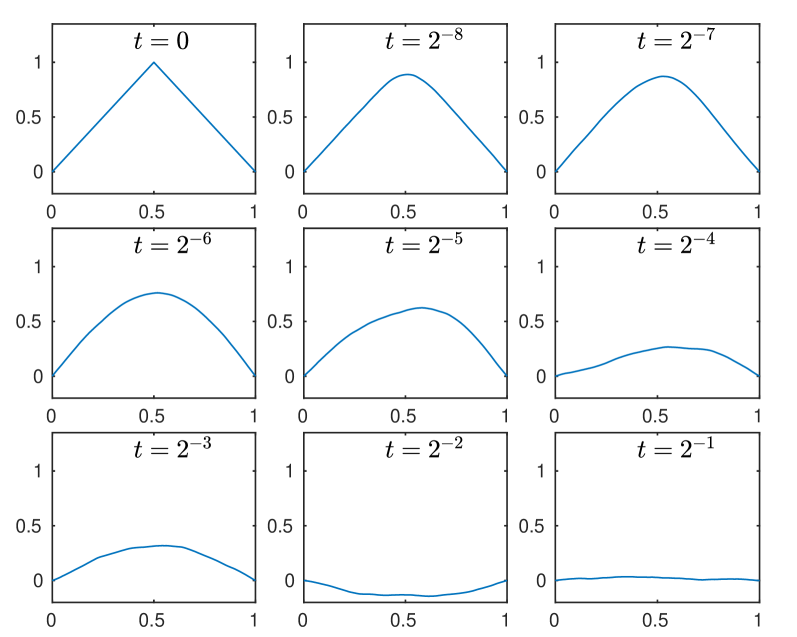
6.2. Linear filtering problems

We consider the filtering problem in Section 5.2 with the linear forcing $f(u)=u$ in the underlying dynamics (35), smoothing parameter $b=1/2$, approximation space parameters $r_{1}=1/4+\upsilon$ and $r_{2}=3/4-\upsilon$ with $\upsilon=10^{-4}$, observation functional

$$H=\delta_{0.5}=\sqrt{2}\sum_{j=1}^{\infty}\sin(j\pi/2)\phi_{j}^{*},$$

observation noise parameter $\Gamma=0.5$, QoI

$$\varphi=1^{*}=\sum_{j\in\mathbb{N}}\frac{\sqrt{2}(1-\cos(j\pi))}{j\pi}\phi_{j}^{*},$$ (55)

and initial data

$$u_{0}(x)=1-2\left|x-\frac{1}{2}\right|=\sum_{j\in\mathbb{N}}(-1)^{j-1}\frac{4\sqrt{2}}{((2j-1)\pi)^{2}}\phi_{2j-1}(x).$$

We note that $H,\varphi\in\mathcal{V}^{*}$ and $u_{0}\in V$. Figure 1 illustrates one exact-in-time simulation of the SPDE.

Refer to caption
Figure 1. Exact-in-time simulation of the SPDE in Section 6.2 over one observation-time interval with spatial resolution $N_{10}=2^{12}$.

By the approximation $\beta=2(r_{2}-r_{1})\approx 2$, application of the error equilibration in Section 5.5.1 yields ($d\gamma_{x}=1$,$\gamma_{t}=1$) for the fully-discrete method and ($d\gamma_{x}=1$, $\gamma_{t}=0$) for the spatially-discrete method. Figure 2 and the left subfigure of Figure 3 display the runtime-to-MSE performance for the spatially-discrete and fully-discrete methods, respectively.

Refer to caption
Figure 2. Runtime-to-MSE comparison for the filtering problem in Section 6.2 using the spatially-discrete method.

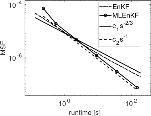
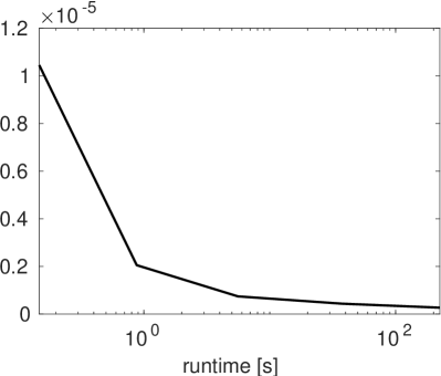
The right subfigure of Figure 3 displays the graph of

$$(\text{Runtime(MLEnKF)},\,\text{MSE(MLEnKF)}\times\text{Runtime(MLEnKF)}/L^{3}),$$

(where MSE(MLEnKF) in the second argument denotes the “MSE” obtained for a given “Runtime”). The numerical observations are consistent with the approximate theoretical predictions (53) and (54).

Refer to caption
Refer to caption
Figure 3. Left: Runtime-to-MSE comparison for the filtering problem in Section 6.2 using the fully-discrete numerical method. Right: Graph of $(\text{Runtime(MLEnKF)},\,\text{MSE(MLEnKF)}\times\text{Runtime(MLEnKF)}/L^{3})$ for the fully-discrete numerical method. Note the y-axis here, and in future such plots, has linear scaling.

The reference-solution sequence $\{\hat{\bar{\mu}}_{n}[\varphi]\}_{n=1}^{N}$ that is needed to estimate the MSE in the above figures, is approximated by Kalman filtering the subspace $\mathcal{V}_{12}\subset\mathcal{V}$, which is an $N_{12}=2^{14}$-dimensional subspace. This yields an accurate approximation, since when the underlying dynamics (35) is linear with Gaussian additive noise, the full-space Kalman filter distribution equals the reference MFEnKF distribution $\hat{\bar{\mu}}$. Furthermore, EnKF and MLEnKF solutions are computed with ensemble particles at no higher spatial resolution than $\mathcal{V}_{9}$ in the cost-to-accuracy studies.

6.3. A nonlinear filtering problem

We seek the mild solution to the following nonlinear SPDE with periodic boundary conditions

$$\begin{split}du&=\left((\Delta-I)u+\sin(\pi u)\right)dt+BdW,\qquad(t,x)\in(0,T]\times(0,1),\\ u(0,x)&=4(x-1/2)^{2}\\ u(t,0)&=u(t,1),\mspace{240.0mu}t\in(0,T],\end{split}$$ (56)

where $W$ and $B$ are described below. Here, the operator $-A=(I-\Delta)$ is defined as a mapping $A:H^{2}(0,1)\cap H^{1}_{\text{per}}(0,1)\to\mathcal{K}=L^{2}(0,1)$, where $H^{1}_{\text{per}}(0,1):=\{f\in H(0,1)\mid(f-f(0))\in H^{1}_{0}(0,1)\}$. The periodic boundary condition is different from the zero-valued boundary condition in (35), and, in order to spectrally decompose $-A$, we now express the base-space $\mathcal{K}=L^{2}(0,1)$ by the closure of the span of the Fourier basis

$$\phi_{k}(x)=\begin{cases}1,&k=1,\\ \sqrt{2}\cos(2k\pi x),&k=2,4,6\ldots\,,\\ \sqrt{2}\sin(2(k-1)\pi x),&k=3,5,7,\ldots\end{cases}$$ (57)

The operator $-A$ is spectrally decomposed by

$$-A\phi_{k}=\lambda_{k}\phi_{k}$$

with

$$\lambda_{k}=\begin{cases}1,&k=1,\\ 1+(2k\pi)^{2},&k=2,4,6,\ldots\,,\\ 1+(2(k-1)\pi)^{2}&k=3,5,7,\ldots\end{cases}$$

As in Section 5.1, we introduce the family of Hilbert spaces parametrized in
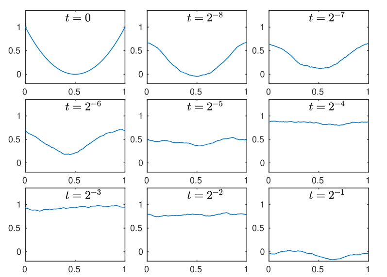
 r𝑟r\in\mathbb{R}

$$\begin{split}\mathcal{K}_{r}\mathrel{\mathop{:}}=D((-A)^{r})=\Big{\{}v:[0,1]\to\mathbb{R}\mid&v\text{ is }\mathcal{B}([0,1])/\mathcal{B}(\mathbb{R})\text{-measurable}\\ &\text{and }\sum_{j\in\mathbb{N}}\lambda^{2r}_{j}\left|\langle\phi_{j},v\rangle_{\mathcal{K}}\right|^{2}<\infty\Big{\}},\end{split}$$

with norm $\|\cdot\|_{\mathcal{K}_{r}}\mathrel{\mathop{:}}=\|(-A)^{r}(\cdot)\|_{\mathcal{K}}$. As smoothing operator $B$, we consider (36) with parameter $b=1/4$, where $W$ denotes an $I_{\mathcal{K}}$-cylindrical Wiener process (both $B$ and $W$ are of course expanded in the currently considered basis (57)). We consider the approximation spaces

$$\mathcal{V}=\mathcal{K}_{0}\quad\text{and}\quad V=\mathcal{K}_{(1-\nu)/2},$$

where $\nu=10^{-4}$, the QoI (55) and the observation operator

$$H=1_{x>0.5}^{*}=\frac{1}{2}\phi_{0}^{*}+\sum_{k=1}^{\infty}\frac{\sqrt{2}}{\pi k}\phi_{2k+1}^{*}.$$

The spectral representation of the initial data

$$u(0,\cdot)=\frac{1}{3}+\sum_{k=1}\frac{2\sqrt{2}}{(\pi k)^{2}}\phi_{2k}(\cdot)$$

implies that $u(0,\cdot)\in\mathcal{K}_{(1-\nu)/2}$. Figure 4 illustrates one simulation of the SPDE by the numerical scheme described below.

Refer to caption
Figure 4. Simulation of the SPDE (56) over one observation-time interval by the numerical scheme in Section 6.3.1 on resolutions $N_{10}=J_{10}=2^{12}$.

By the Lipschitz-continuity of the reaction term, it follows that Assumption 3 is fulfilled. Moreover, the well-posedness theory for the zero-valued boundary condition for the SPDE (35) extends to the current setting, and so does the theory for the fully-discrete exponential Euler method in Section 5.4, cf. [28].

6.3.1. Numerical scheme

We apply the coupled fully discrete approximation method described in Section 5.4, but, due to the nonlinearity of the reaction term $f(u)=\sin(\pi u)$, the spectral representation in the coupled scheme (42) and (44) needs to be approximated. Namely, the approximation of $[(f_{\ell}(U_{\ell,k}))^{(1)},\ldots,(f_{\ell}(U_{\ell,k}))^{(N_{\ell})}]$ is obtained by application of the fast Fourier transform (FFT) as follows:

  1. 1.

    Given the spectral representation $[U_{\ell,k}^{(1)},\ldots,U_{\ell,k}^{(N_{\ell})}]$ compute the physical-space-on-uniform-mesh representation by the inverse FFT

    $$[U_{\ell,k}(0),U_{\ell,k}(1/N_{\ell}),\ldots,U_{\ell,k}(1-N_{\ell}^{-1})]=\text{IFFT}[U_{\ell,k}^{(1)},\ldots,U_{\ell,k}^{(N_{\ell})}].$$
  2. 2.

    Evaluate the nonlinear reaction term in physical space and approximate the spectral representation by FFT

    $$[(f_{\ell}(U_{\ell,k}))^{(1)},\ldots,(f_{\ell}(U_{\ell,k}))^{(N_{\ell})}]\\ \approx\text{FFT}[f(U_{\ell,k}(0)),f(U_{\ell,k}(1/N_{\ell})),\ldots,f(U_{\ell,k}(1-N_{\ell}^{-1}))].$$

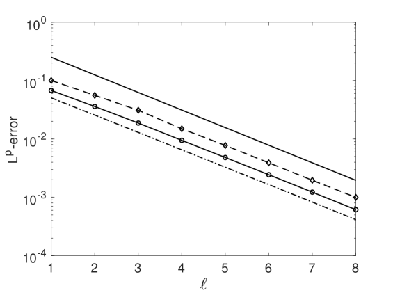
The spectral approximation of the coarse-level reaction term is obtained analogously. Due to the FFT approximation error in step 2. above, we cannot directly obtain the rate parameter $\beta$ from the analysis in Section 5.4. To infer $\beta$, we instead perform numerical studies of the $L^{p}(\Omega,\mathcal{V})$-convergence rate of the coupled-level difference of the FFT-based fully-discrete method $\widetilde{\Psi}^{\ell}(u)-\widetilde{\Psi}^{\ell-1}(u)$ towards 00, where the expectation is estimated with the Monte Carlo method with $M=10^{5}$ samples:

$$\left(\frac{1}{M}\sum_{i=1}^{M}\|\widetilde{\Psi}^{\ell}(u_{0};\omega_{i})-\widetilde{\Psi}^{\ell-1}(u_{0};\omega_{i})\|_{\mathcal{V}}^{p}\right)^{1/p}\approx\|\widetilde{\Psi}^{\ell}(u)-\widetilde{\Psi}^{\ell-1}(u)\|_{L^{p}(\Omega,\mathcal{V})}$$ (58)

Recalling that $h_{\ell}^{-1}\eqsim N_{\ell}\eqsim J_{\ell}=2^{2+\ell}$ for the numerical solver $\widetilde{\Psi}^{\ell}$, we infer from the results of the numerical study (58), which is provided in Figure 5, that

$$\|\widetilde{\Psi}^{\ell}(u)-\Psi(u)\|_{p}\lessapprox h_{\ell}^{\beta/2}$$ (59)

with $\beta=2$. Further numerical studies, which we do not include here, indicate that the right hand side of (59) may be decomposed into $\mathcal{O}(N_{\ell}^{-1}+J_{\ell}^{-1})$. On the basis of these observations, the configuration of discretization parameters for this problem, $N_{\ell}\eqsim J_{\ell}$, is in alignment with the efficiency-optimized error equilibration strategy in Section 5.5.1.

Refer to caption
Figure 5. Numerical estimates of the error $\|\widetilde{\Psi}^{\ell}(u_{0})-\widetilde{\Psi}^{\ell-1}(u_{0})\|_{p}$ by the Monte Carlo method (58) for $p=2$ (dash-dot), $p=4$ (solid-circle), and $p=8$ (dash-diamond). The solid line represents the reference function $f(\ell)=2^{-(\ell+1)}$.

The left subfigure in Figure 6 displays the results of the runtime-to-MSE studies of EnKF and MLEnKF.

Refer to caption
Refer to caption
Figure 6. Left: Runtime-to-MSE for the nonlinear filtering problem in Section 6.3.1 using the fully-discrete method. Right: Graph of $(\text{Runtime(MLEnKF)},\,\text{MSE(MLEnKF)}\times\text{Runtime(MLEnKF)}/L^{3})$ for the fully-discrete method.

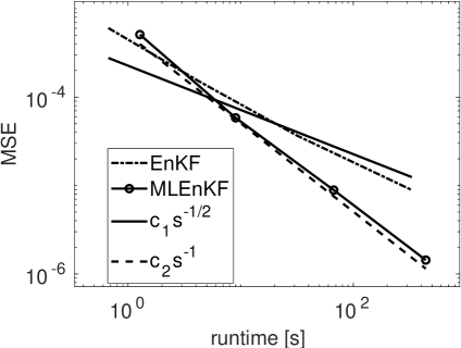
As pseudo-reference solution, we use the approximation

$$\frac{1}{200}\sum_{i=1}^{200}\mu^{\rm{ML}}_{n,i}[\varphi]\approx\hat{\bar{\mu}}_{n}[\varphi],\quad n=1,2,\ldots,40,$$

with the MLEnKF estimator $\mu^{\rm{ML}}_{n,i}[\varphi]$ here being computed on a finer resolution than all those considered in the runtime-to-MSE study. The right subfigure in Figure 6 displays the graph of

$$(\text{Runtime(MLEnKF)},\,\text{MSE(MLEnKF)}\times\text{Runtime(MLEnKF)}/L^{3}).$$

Once again, the numerical observations are consistent with the theoretical asymptotical behavior predicted by (53) and (54).

Remark 9 (MLEnKF versus Multilevel particle filters).

To the best of our knowledge, there does not exist a general multilevel particle filter for SPDE to this date. When the effective dimension on level $\ell$ is $N_{\ell}$, the general requirement for particle filters is that the ensemble size on that level is bounded from below by $ce^{N_{\ell}}$ particles, for some constant $c>0$. Effective dimension refers to the dimension of the space over which importance sampling needs to be performed [3, 10, 1]. For example, in the case of full observations, the effective dimension can be equal to the state-space dimension. For MLEnKF, on the other hand, the level $\ell$ ensemble size is always bounded from above by $\mathcal{O}(L^{2}N_{\ell}^{(\beta-d\gamma_{x}-\gamma_{t})/(2d)})$, even with full observations. The set of MLEnKF-tractable problems is therefore substantially larger than the set of problems tractable by particle filters.

7. Conclusion

We have presented the design and analysis of a multilevel EnKF method for infinite-dimensional spatio-temporal processes depending on a hierarchical decomposition of both the spatial and the temporal parameters. We have proved theoretically and provided numerical evidence that under suitable assumptions, a similar asymptotic cost-to-accuracy is obtained for MLEnKF as that one obtains for standard multilevel Monte Carlo methods. This result has potential for broad impact across application areas in which there has been a recent explosion of interest in EnKF, for example weather prediction and subsurface exploration.

Appendix A Marcinkiewicz–Zygmund inequalities for separable Hilbert spaces

In order to prove Lemma 5, we will need the following two lemmas for extending the Marcinkiewicz–Zygmund inequality from finite-dimensional state-spaces to separable Hilbert spaces.

Lemma 9.

[34, Theorem 5.2] Let $2\leq p<\infty$ and $X_{i}\in L^{p}(\Omega,\mathcal{V})$ be i.i.d. samples of $X\in L^{p}(\Omega,\mathcal{V})$. Then

$$\|E_{M}[X]-\mathbb{E}\mspace{-2.0mu}\left[X\right]\|_{L^{p}(\Omega,\mathcal{V})}\leq\frac{c_{p}}{\sqrt{M}}\|X-\mathbb{E}\mspace{-2.0mu}\left[X\right]\|_{L^{p}(\Omega,\mathcal{V})}$$ (60)

where $c_{p}$ only depends on $p$.

Proof.

Let $r_{1},r_{2},\ldots$ denote a sequence of real-valued i.i.d. random variables with $P(r_{i}=\pm 1)=1/2$. A Banach space $\mathcal{K}$ is said to be of R-type $q$ if there exists a $c>0$ such that for every $\bar{n}\in\mathbb{N}$ and for all (deterministic) $x_{1},x_{2},\ldots,x_{\bar{n}}\in\mathcal{K}$,

$$\mathbb{E}\mspace{-2.0mu}\left[\Big{\|}\sum_{i=1}^{\bar{n}}r_{i}x_{i}\Big{\|}_{\mathcal{K}}\right]\leq c\left(\sum_{i=1}^{\bar{n}}\|x_{i}\|_{\mathcal{K}}^{q}\right)^{1/q}.$$

It is clear that all Hilbert spaces (and for our interest $\mathcal{V}$, in particular) are of R-type 2, since their norms are induced by an inner product. Following the proofs of [50, Proposition 2.1 and Corollary 2.1], let $\{X_{i}^{\prime}\}$ denote an additional sequence of i.i.d. samples of $X\in L^{p}(\Omega,\mathcal{V})$ for which the collection of r.v. $\{X_{i}\}\cup\{X_{i}^{\prime}\}$ also is i.i.d. Introducing the symmetrization $\widetilde{X}_{i}\mathrel{\mathop{:}}=(X_{i}-X_{i}^{\prime})$, and noting that

$$\mathbb{E}\mspace{-2.0mu}\left[X_{i}-\mathbb{E}\mspace{-2.0mu}\left[X\right]\right]=\mathbb{E}\mspace{-2.0mu}\left[\mathbb{E}\mspace{-2.0mu}\left[\widetilde{X}_{i}\mid X_{i}\right]\right],$$

we derive by the conditional Jensen’s inequality that

$$\mathbb{E}\mspace{-2.0mu}\left[\left\|\sum_{i=1}^{\bar{n}}X_{i}-\mathbb{E}\mspace{-2.0mu}\left[X\right]\right\|_{\mathcal{V}}^{p}\right]\leq\mathbb{E}\mspace{-2.0mu}\left[\left\|\mathbb{E}\mspace{-2.0mu}\left[\sum_{i=1}^{\bar{n}}\widetilde{X}_{i}\Bigg{|}\{X_{i}\}_{i=1}^{\bar{n}}\right]\right\|_{\mathcal{V}}^{p}\right]\\ \leq\mathbb{E}\mspace{-2.0mu}\left[\left\|\sum_{i=1}^{\bar{n}}\widetilde{X}_{i}\right\|_{\mathcal{V}}^{p}\right]=\mathbb{E}\mspace{-2.0mu}\left[\left\|\sum_{i=1}^{\bar{n}}r_{i}\widetilde{X}_{i}\right\|_{\mathcal{V}}^{p}\right]\leq c\mathbb{E}\mspace{-2.0mu}\left[\left(\sum_{i=1}^{\bar{n}}\left\|\widetilde{X}_{i}\right\|_{\mathcal{V}}^{2}\right)^{p/2}\right]\\ \leq c2^{p}\,\mathbb{E}\mspace{-2.0mu}\left[\left(\sum_{i=1}^{\bar{n}}\left\|X_{i}-\mathbb{E}\mspace{-2.0mu}\left[X\right]\right\|_{\mathcal{V}}^{2}\right)^{p/2}\right].$$

And by another application of Hölder’s inequality,

$$\begin{split}\mathbb{E}\mspace{-2.0mu}\left[\left\|\sum_{i=1}^{M}\frac{X_{i}-\mathbb{E}\mspace{-2.0mu}\left[X\right]}{M}\right\|_{\mathcal{V}}^{p}\right]&\leq\hat{c}M^{-p}\mathbb{E}\mspace{-2.0mu}\left[\left(\sum_{i=1}^{M}\left\|X_{i}-\mathbb{E}\mspace{-2.0mu}\left[X\right]\right\|_{\mathcal{V}}^{2}\right)^{p/2}\right]\\ &\leq\hat{c}M^{-p/2}\mathbb{E}\mspace{-2.0mu}\left[\left\|X-\mathbb{E}\mspace{-2.0mu}\left[X\right]\right\|_{\mathcal{V}}^{p}\right].\end{split}$$

Lemma 10.

Let $X,Y\in L^{p}(\Omega,\mathcal{V})$, for some $p\geq 2$. Then, for any $1\leq r,s\leq\infty$ satisfying $1/r+1/s=1$, it holds that

$$\begin{split}\|\mathrm{Cov}_{M}[X,Y]-\mathrm{Cov}[X,Y]\|_{L^{p}(\Omega,\mathcal{V}\otimes\mathcal{V})}\leq\frac{c}{\sqrt{M}}\|X\|_{L^{pr}(\Omega,\mathcal{V})}\|Y\|_{L^{ps}(\Omega,\mathcal{V})}\end{split}$$

where the upper bound for the constant $c=\dfrac{M}{M-1}\bigg{(}2c_{p}+\dfrac{c_{pr}c_{ps}+1}{\sqrt{M}}\bigg{)}$ only depends on $r,s$ and $p$.

Proof.

Since $\mathrm{Cov}[X,Y]=\mathrm{Cov}[X-\mathbb{E}\mspace{-2.0mu}\left[X\right],Y-\mathbb{E}\mspace{-2.0mu}\left[Y\right]]$ and $\mathrm{Cov}_{M}[X,Y]=\mathrm{Cov}_{M}[X-\mathbb{E}\mspace{-2.0mu}\left[X\right],Y-\mathbb{E}\mspace{-2.0mu}\left[Y\right]]$, cf. (7), we may without loss of generality assume that $\mathbb{E}\mspace{-2.0mu}\left[X\right]=\mathbb{E}\mspace{-2.0mu}\left[Y\right]=0$. Using the triangle inequality,

$$\begin{split}&\frac{M-1}{M}\|\mathrm{Cov}_{M}[X,Y]-\mathrm{Cov}[X,Y]\|_{p}\\ &\leq\|E_{M}[X\otimes Y]-\mathbb{E}\mspace{-2.0mu}\left[X\otimes Y\right]\|_{p}+\|E_{M}[X]\otimes E_{M}[Y]\|_{p}+\frac{1}{M}\|\mathbb{E}\mspace{-2.0mu}\left[X\otimes Y\right]\|_{\mathcal{V}\otimes\mathcal{V}}.\end{split}$$

Estimate (60) and Hölder’s inequality yield

$$\begin{split}\|E_{M}[X\otimes Y]-\mathbb{E}\mspace{-2.0mu}\left[X\otimes Y\right]\|_{p}&\leq\frac{c_{p}}{\sqrt{M}}\|X\otimes Y-\mathbb{E}\mspace{-2.0mu}\left[X\otimes Y\right]\|_{p}\\ &\leq\frac{2c_{p}}{\sqrt{M}}\|X\otimes Y\|_{p}\leq\frac{2c_{p}}{\sqrt{M}}\|X\|_{pr}\|Y\|_{ps}.\end{split}$$

Similarly, since $\mathbb{E}\mspace{-2.0mu}\left[X\right]=\mathbb{E}\mspace{-2.0mu}\left[Y\right]=0$ by assumption, we obtain by (60) and Hölder’s inequality

$$\begin{split}\|E_{M}[X]\otimes E_{M}[Y]\|_{p}\leq\|E_{M}[X]\|_{pr}\|E_{M}[Y]\|_{ps}\leq\frac{c_{pr}c_{ps}}{M}\|X\|_{pr}\|Y\|_{ps}.\end{split}$$

And, finally, for the last term

$$\frac{1}{M}\|\mathbb{E}\mspace{-2.0mu}\left[X\otimes Y\right]\|_{\mathcal{V}\otimes\mathcal{V}}\leq\frac{1}{M}\|X\otimes Y\|_{L^{1}(\Omega,\mathcal{V}\otimes\mathcal{V})}\leq\frac{1}{M}\|X\|_{L^{pr}(\Omega,\mathcal{V})}\|Y\|_{L^{ps}(\Omega,\mathcal{V})}.$$

Appendix B Proof of Lemma 8

Proof.

Introducing the function $g:(1,\infty)\times(0,\infty)\to\mathbb{R}$ defined by

$$g(\lambda,s)=e^{-\lambda s}+\frac{1-e^{-\lambda s}}{\lambda},$$

consecutive iterations of the scheme (42) for $j\leq N_{m}$ yield

$$\begin{split}U^{(j)}_{m,J_{m}}&=g(\lambda_{j},\Delta t_{m})U^{(j)}_{m,J_{m}-1}+R_{m,J_{m}-1}\\ &=\left(g(\lambda_{j},\Delta t_{m})\right)^{2}U_{m,J_{m}-2}^{(j)}+g(\lambda_{j},\Delta t_{m})R_{m,J_{m}-2}^{(j)}+R_{m,J_{m}-1}^{(j)}\\ &=\ldots\\ &=\left(g(\lambda_{j},\Delta t_{m})\right)^{J_{m}}U_{m,0}^{(j)}+\sum_{k=0}^{J_{m}-1}\left(g(\lambda_{j},\Delta t_{m})\right)^{J_{m}-(k+1)}R_{m,k}^{(j)},\end{split}$$

where we recall that the initial data is given by $U_{m,0}=\mathcal{P}_{m}\bar{u}_{0}$ with $\bar{u}_{0}\in L^{2}(\Omega,\mathcal{V})$. And since $J_{m}=2J_{m-1}$, consecutive iterations of the coupled coarse scheme (44) for $j\leq N_{m-1}$ yield

$$\begin{split}U^{(j)}_{m-1,J_{m-1}}&=g(\lambda_{j},\Delta t_{m-1})U^{(j)}_{m-1,J_{m-1}-1}+e^{-\lambda_{j}\Delta t_{m}}R_{m,J_{m}-2}^{(j)}+R_{m,J_{m}-1}^{(j)}\\ &=\left(g(\lambda_{j},\Delta t_{m-1})\right)^{2}U^{(j)}_{m-1,J_{m-1}-2}\\ &\quad+g(\lambda_{j},\Delta t_{m-1})\left(e^{-\lambda_{j}\Delta t_{m}}R_{m,J_{m}-4}^{(j)}+R_{m,J_{m}-3}^{(j)}\right)\\ &\quad+e^{-\lambda_{j}\Delta t_{m}}R_{m,J_{m}-2}^{(j)}+R_{m,J_{m}-1}^{(j)}\\ &=\ldots\\ &=\left(g(\lambda_{j},\Delta t_{m-1})\right)^{J_{m-1}}U_{m-1,0}^{(j)}\\ &+\sum_{k=0}^{J_{m-1}-1}\left(g(\lambda_{j},\Delta t_{m-1})\right)^{J_{m-1}-(k+1)}\left(e^{-\lambda_{j}\Delta t_{m}}R_{m,2k}^{(j)}+R_{m,2k+1}^{(j)}\right).\end{split}$$

The $j$-th mode final time difference of the coupled solutions for $j\leq N_{m-1}$ thus becomes

$$\begin{split}&U^{(j)}_{m,J_{m}}-U^{(j)}_{m-1,J_{m-1}}=\left(\left(g(\lambda_{j},\Delta t_{m})\right)^{2J_{m-1}}-\left(g(\lambda_{j},\Delta t_{m-1})\right)^{J_{m-1}}\right)U_{\ell,0}^{(j)}\\ &+\sum_{k=0}^{J_{m-1}-1}\left(\left(g(\lambda_{j},\Delta t_{m})\right)^{2k}-\left(g(\lambda_{j},\Delta t_{m-1})\right)^{k}\right)R_{m,J_{m}-2k+1}^{(j)}\\ &+\sum_{k=0}^{J_{m-1}-1}\Bigg{(}\left(g(\lambda_{j},\Delta t_{m})\right)^{2k}g(\lambda_{j},\Delta t_{m})-\left(g(\lambda_{j},\Delta t_{m-1})\right)^{k}e^{-\lambda_{j}\Delta t_{m}}\Bigg{)}R_{m,J_{m}-2(k+1)}^{(j)}\\ &=\mathrel{\mathop{:}}I_{m,j,1}+I_{m,j,2}+I_{m,j,3}.\end{split}$$ (61)

For bounding these three terms, we need to estimate the difference between powers of $\left(g(\lambda_{j},\Delta t_{m})\right)^{2}$ and $g(\lambda_{j},\Delta t_{m-1})$. Note first that

$$\begin{split}\left(g(\lambda_{j},\Delta t_{m})\right)^{2}&=e^{-2\lambda_{j}\Delta t_{m}}+2e^{-\lambda_{j}\Delta t_{m}}\frac{1-e^{-\lambda_{j}\Delta t_{m}}}{\lambda_{j}}+\left(\frac{1-e^{-\lambda_{j}\Delta t_{m}}}{\lambda_{j}}\right)^{2}\\ &=\underbrace{e^{-\lambda_{j}\Delta t_{m-1}}+\frac{1-e^{-\lambda_{j}\Delta t_{m-1}}}{\lambda_{j}}}_{=g(\lambda_{j},\Delta t_{m-1})}+(1-\lambda_{j})\left(\frac{1-e^{-\lambda_{j}\Delta t_{m}}}{\lambda_{j}}\right)^{2}.\end{split}$$ (62)
Remark 10.

Equations (61) and (62) show that to leading order, the additive noise from two consecutive iterations of the fine scheme equals the additive noise from one corresponding iteration of the coupled coarse scheme. The strong coupling of the coarse and fine schemes is crucial for achieving the order 1 a priori time discretization convergence rate.

Since $\inf_{j\in\mathbb{N}}\lambda_{j}=\lambda_{1}>1$, it holds for all $j\in\mathbb{N}$ that

$$\left(g(\lambda_{j},\Delta t_{m})\right)^{2}<g(\lambda_{j},\Delta t_{m-1})<1$$ (63)

and

$$\left|\left(g(\lambda_{j},\Delta t_{m})\right)^{2}-g(\lambda_{j},\Delta t_{m-1})\right|<\left(1-e^{-\lambda_{j}\Delta t_{m}}\right)\frac{1-e^{-\lambda_{j}\Delta t_{m}}}{\lambda_{j}}\leq\left(1-e^{-\lambda_{j}\Delta t_{m}}\right)\Delta t_{m}.$$

By the mean value theorem, it holds for any $j,k\geq 1$ that

$$\begin{split}&\left|\left(g(\lambda_{j},\Delta t_{m})\right)^{2k}-\left(g(\lambda_{j},\Delta t_{m-1})\right)^{k}\right|\leq\left(g(\lambda_{j},\Delta t_{m-1})\right)^{k-1}k\left(1-e^{-\lambda_{j}\Delta t_{m}}\right)\Delta t_{m}.\end{split}$$ (64)

Furthermore,

$$\sup_{\lambda\geq\lambda_{1}}\lambda e^{-\lambda s}\leq\frac{e^{-1}}{s},\quad\text{for any}\quad s>0.$$ (65)

By (63), (64),, (65), the mean value theorem and recalling that $\Delta t_{m-1}=2\Delta t_{m}$, it holds for any $1<k\leq J_{m-1}$ and $j\geq 1$ and some $\theta_{jk}\in[0,1]$ that

$$\begin{split}&\left|\left(g(\lambda_{j},\Delta t_{m})\right)^{2k}-\left(g(\lambda_{j},\Delta t_{m-1})\right)^{k}\right|\leq\left(e^{-\lambda_{j}\Delta t_{m-1}}+\frac{1-e^{-\lambda_{j}\Delta t_{m-1}}}{\lambda_{j}}\right)^{k-1}k\lambda_{j}\Delta t_{m}^{2}\\ &\leq e^{-\lambda_{j}(k-1)\Delta t_{m-1}}k\lambda_{j}\Delta t_{m}^{2}\\ &+\left(e^{-\lambda_{j}\Delta t_{m-1}}+\theta_{jk}\frac{1-e^{-\lambda_{j}\Delta t_{m-1}}}{\lambda_{j}}\right)^{k-2}(k-1)k\Delta t_{m-1}\Delta t_{m}^{2}\\ &\leq\frac{e^{-1}k}{(k-1)\Delta t_{m-1}}\Delta t_{m}^{2}+\frac{T^{2}}{2}\Delta t_{m}\\ &\leq\frac{1+T^{2}}{2}\Delta t_{m}.\end{split}$$ (66)

From (66), we conclude that for $j\leq N_{m-1}$,

$$\left|I_{m,j,1}\right|\leq\frac{1+T^{2}}{2}|U_{\ell,0}^{(j)}|\Delta t_{m}.$$

For bounding the terms $I_{m,j,2}$ and $I_{m,j,3}$, note by (61) that both terms are linear combinations of i.i.d. Gaussians from the sequence

$$R^{(j)}_{m,k}\sim N\left(0,\frac{1-e^{-\lambda_{j}\Delta t_{m}}}{2\lambda_{j}^{1+2b}}\right),\quad k=0,1,\ldots,J_{m}-1,$$

cf. (43), and hence, both terms mean zero-valued Gaussians. Furthermore, $I_{m,j,2}$ and $I_{m,j,3}$ are mutually independent as any summand of the former term is independent of any summand from the latter. Consequently, $I_{m,j,2}+I_{m,j,3}$ is a mean zero-valued Gaussian with variance

$$\mathbb{E}\mspace{-2.0mu}\left[(I_{m,j,2}+I_{m,j,3})^{2}\right]=\mathbb{E}\mspace{-2.0mu}\left[I_{m,j,2}^{2}\right]+\mathbb{E}\mspace{-2.0mu}\left[I_{m,j,3}^{2}\right].$$

By the mutual independence of all terms in $I_{m,j,2}$, it holds for $j\leq N_{m-1}$ that

$$\begin{split}\mathbb{E}\mspace{-2.0mu}\left[I_{m,j,2}^{2}\right]&=\sum_{k=0}^{J_{m-1}-1}\left(\left(g(\lambda_{j},\Delta t_{m})\right)^{2k}-\left(g(\lambda_{j},\Delta t_{m-1})\right)^{k}\right)^{2}\mathbb{E}\mspace{-2.0mu}\left[\left(R_{m,J_{m}-2k+1}^{(j)}\right)^{2}\right]\\ &\leq\frac{1-e^{-\lambda_{j}\Delta t_{m}}}{2\lambda_{j}^{1+2b}}\sum_{k=0}^{\infty}\left(\left(g(\lambda_{j},\Delta t_{m})\right)^{2k}-\left(g(\lambda_{j},\Delta t_{m-1})\right)^{k}\right)^{2}\\ &=\frac{1-e^{-\lambda_{j}\Delta t_{m}}}{2\lambda_{j}^{1+2b}}\sum_{k=0}^{\infty}\Bigg{[}\left(g(\lambda_{j},\Delta t_{m})\right)^{4k}+\left(g(\lambda_{j},\Delta t_{m-1})\right)^{2k}\\ &\qquad\qquad\qquad\qquad\qquad-2\left(\left(g(\lambda_{j},\Delta t_{m})\right)^{2}g(\lambda_{j},\Delta t_{m-1})\right)^{k}\Bigg{]}.\end{split}$$ (67)

By the strict inequality (63), we are dealing with three sums of geometric series:

$$\sum_{k=0}^{\infty}\left(\left(g(\lambda_{j},\Delta t_{m})\right)^{2}g(\lambda_{j},\Delta t_{m-1})\right)^{k}=\frac{1}{1-g(\lambda_{j},\Delta t_{m-1})\left(g(\lambda_{j},\Delta t_{m})\right)^{2}},$$
$$\begin{split}\sum_{k=0}^{\infty}\left(g(\lambda_{j},\Delta t_{m})\right)^{4k}&=\frac{1}{1-\left(g(\lambda_{j},\Delta t_{m})\right)^{4}},\end{split}$$

and

$$\begin{split}\sum_{k=0}^{\infty}\left(g(\lambda_{j},\Delta t_{m-1})\right)^{2k}&=\frac{1}{1-\left(g(\lambda_{j},\Delta t_{m-1})\right)^{2}}\,\,.\end{split}$$

By applying $g(\lambda_{j},\Delta t_{m})<g(\lambda_{j},\Delta t_{m-1})<1$ and the mean value theorem,

$$\begin{split}&\sum_{k=0}^{\infty}\left(g(\lambda_{j},\Delta t_{m})\right)^{4k}+\left(g(\lambda_{j},\Delta t_{m-1})\right)^{2k}=\frac{2-\left(g(\lambda_{j},\Delta t_{m})\right)^{4}-\left(g(\lambda_{j},\Delta t_{m-1})\right)^{2}}{\left(1-\left(g(\lambda_{j},\Delta t_{m})\right)^{4}\right)\left(1-\left(g(\lambda_{j},\Delta t_{m-1})\right)^{2}\right)}\\ &=\frac{2\left(1-\left(g(\lambda_{j},\Delta t_{m})\right)^{2}g(\lambda_{j},\Delta t_{m-1})\right)-\left(\left(g(\lambda_{j},\Delta t_{m})\right)^{2}-g(\lambda_{j},\Delta t_{m-1})\right)^{2}}{\left(1-\left(g(\lambda_{j},\Delta t_{m})\right)^{2}g(\lambda_{j},\Delta t_{m-1})\right)^{2}-\left(\left(g(\lambda_{j},\Delta t_{m})\right)^{2}-g(\lambda_{j},\Delta t_{m-1})\right)^{2}}\\ &\leq\frac{2}{1-g(\lambda_{j},\Delta t_{m-1})\left(g(\lambda_{j},\Delta t_{m})\right)^{2}}+\frac{2}{\left(1-g(\lambda_{j},\Delta t_{m})\right)^{3}}\frac{\left(1-e^{-\lambda_{j}\Delta t_{m}}\right)^{4}}{\lambda_{j}^{2}}\,\end{split}$$

where the second summand in the last inequality follows from (62). By (67), we obtain that for all $j\leq N_{m-1}$,

$$\begin{split}\mathbb{E}\mspace{-2.0mu}\left[I_{m,j,2}^{2}\right]&\leq\frac{1}{\left(1-g(\lambda_{j},\Delta t_{m})\right)^{3}}\frac{\left(1-e^{-\lambda_{j}\Delta t_{m}}\right)^{5}}{\lambda_{j}^{3+2b}}\\ &\leq\frac{\lambda_{j}^{3}}{(\lambda_{j}-1)^{3}\left(1-e^{-\lambda_{j}\Delta t_{m}}\right)^{3}}\frac{\left(1-e^{-\lambda_{j}\Delta t_{m}}\right)^{3}}{\lambda_{j}^{1+2b}}\Delta t_{m}^{2}\\ &\leq\left(\frac{\lambda_{1}}{\lambda_{1}-1}\right)^{3}\frac{\Delta t_{m}^{2}}{\lambda_{j}^{1+2b}}.\end{split}$$

The last term is bounded by a similar argument: For all $j\leq N_{m-1}$,

$$\begin{split}&\mathbb{E}\mspace{-2.0mu}\left[I_{m,j,3}^{2}\right]=\sum_{k=0}^{J_{m-1}-1}\Bigg{(}\left(g(\lambda_{j},\Delta t_{m})\right)^{2k}\left(e^{-\lambda_{j}\Delta t_{m}}+\frac{1-e^{-\lambda_{j}\Delta t_{m}}}{\lambda_{j}}\right)\\ &\qquad\qquad-\left(g(\lambda_{j},\Delta t_{m-1})\right)^{k}e^{-\lambda_{j}\Delta t_{m}}\Bigg{)}^{2}\mathbb{E}\mspace{-2.0mu}\left[\left(R_{m,J_{m}-2(k+1)}^{(j)}\right)^{2}\right]\\ &\leq\frac{1-e^{\lambda_{j}\Delta t_{m}}}{\lambda_{j}^{1+2b}}\sum_{k=0}^{\infty}\Bigg{[}\left(\left(g(\lambda_{j},\Delta t_{m})\right)^{2k}-\left(g(\lambda_{j},\Delta t_{m-1})\right)^{k}\right)^{2}\\ &\qquad\qquad\qquad\qquad\qquad\qquad+\left(g(\lambda_{j},\Delta t_{m})\right)^{2k}\left(\frac{1-e^{\lambda_{j}\Delta t_{m}}}{\lambda_{j}}\right)^{2}\Bigg{]}\\ &\leq 3\left(\frac{\lambda_{1}}{\lambda_{1}-1}\right)^{3}\frac{\Delta t_{m}^{2}}{\lambda_{j}^{1+2b}}.\end{split}$$

Here, the last inequality follows by observing that as for $\mathbb{E}\mspace{-2.0mu}\left[I_{m,j,2}^{2}\right]$,

$$\frac{1-e^{\lambda_{j}\Delta t_{m}}}{\lambda_{j}^{1+2b}}\sum_{k=0}^{\infty}\left(\left(g(\lambda_{j},\Delta t_{m})\right)^{2k}-\left(g(\lambda_{j},\Delta t_{m-1})\right)^{k}\right)^{2}\leq 2\left(\frac{\lambda_{1}}{\lambda_{1}-1}\right)^{3}\frac{\Delta t^{2}_{m}}{\lambda_{j}^{1+2b}},$$

and

$$\begin{split}\frac{\left(1-e^{\lambda_{j}\Delta t_{m}}\right)^{3}}{\lambda_{j}^{3+2b}}\sum_{k=0}^{\infty}\left(g(\lambda_{j},\Delta t_{m})\right)^{2k}&\leq\frac{(1-e^{\lambda_{j}\Delta t_{m}})}{\lambda_{j}^{1+2b}}\frac{1}{1-g(\lambda_{j},\Delta t_{m})}\Delta t^{2}_{m}\\ &=\frac{(1-e^{\lambda_{j}\Delta t_{m}})}{\lambda_{j}^{1+2b}}\frac{\lambda_{j}}{(\lambda_{j}-1)(1-e^{\lambda_{j}\Delta t_{m}})}\Delta t^{2}_{m}\\ &\leq\frac{\lambda_{1}}{\lambda_{1}-1}\frac{\Delta t^{2}_{m}}{\lambda_{j}^{1+2b}}\leq\left(\frac{\lambda_{1}}{\lambda_{1}-1}\right)^{3}\frac{\Delta t^{2}_{m}}{\lambda_{j}^{1+2b}}.\end{split}$$

Appendix C Additional proofs for completeness

Proof of Lemma 2.

Recalling the notation $R_{n}^{\rm ML}=C^{\rm ML}_{n}H^{*}$ and introducing the auxiliary operator $\bar{R}_{n}\mathrel{\mathop{:}}=\bar{C}_{n}H^{*}$, we have

$$\begin{split}\bar{K}_{n}-K^{\rm ML}_{n}&=\bar{R}_{n}(H\bar{R}_{n}+\Gamma)^{-1}-R^{\rm ML}_{n}((HR_{n}^{\rm ML})^{+}+\Gamma)^{-1}\\ &=\bar{R}_{n}((H\bar{R}_{n}+\Gamma)^{-1}-((HR_{n}^{\rm ML})^{+}+\Gamma)^{-1})\\ &\quad+(\bar{C}_{n}-C^{\rm ML}_{n})H^{*}((HR^{\rm ML}_{n})^{+}+\Gamma)^{-1}.\end{split}$$

Using the equality

$$(H\bar{R}_{n}+\Gamma)^{-1}-((HR_{n}^{\rm ML})^{+}+\Gamma)^{-1}=(H\bar{R}_{n}+\Gamma)^{-1}((HR_{n}^{\rm ML})^{+}-H\bar{R}_{n})((HR^{\rm ML}_{n})^{+}+\Gamma)^{-1},$$

we further obtain

$$\begin{split}\bar{K}_{n}-K^{\rm ML}_{n}&=\bar{R}_{n}(H\bar{R}_{n}+\Gamma)^{-1}((HR_{n}^{\rm ML})^{+}-H\bar{R}_{n})((HR^{\rm ML}_{n})^{+}+\Gamma)^{-1}\\ &\quad+(\bar{C}_{n}-C^{\rm ML}_{n})H^{*}((HR^{\rm ML}_{n})^{+}+\Gamma)^{-1}\\ &=\bar{K}_{n}((HR_{n}^{\rm ML})^{+}-H\bar{R}_{n})((HR^{\rm ML}_{n})^{+}+\Gamma)^{-1}\\ &\quad+(\bar{C}_{n}-C^{\rm ML}_{n})H^{*}((HR^{\rm ML}_{n})^{+}+\Gamma)^{-1}.\end{split}$$

Next, since $(HR^{\rm ML}_{n})^{+}$ and $\Gamma$ respectively are positive semi-definite and positive definite,

$$|((HR^{\rm ML}_{n})^{+}+\Gamma)^{-1}|\leq|\Gamma^{-1}|<\infty,$$

and it follows by inequality (23) and

$$\begin{split}|(HR_{n}^{\rm ML})^{+}-H\bar{R}_{n}|&\leq|(HR_{n}^{\rm ML})^{+}-HR_{n}^{\rm ML}|+|H(R_{n}^{\rm ML}-\bar{R}_{n})|\\ &=|(HR_{n}^{\rm ML})^{+}-HR_{n}^{\rm ML}|+|H(C_{n}^{\rm ML}-\bar{C}_{n})H^{*}|\end{split}$$

that

$$\begin{split}\left\|\bar{K}_{n}-K^{\mathrm{ML}}_{n}\right\|_{L(\mathbb{R}^{m},\mathcal{V})}&\leq\left(1+2\left\|\bar{K}_{n}\right\|_{L(\mathbb{R}^{m},\mathcal{V})}\left\|H\right\|_{L(\mathcal{V},\mathbb{R}^{m})}\right)\\ &\times|\Gamma^{-1}|\left\|H\right\|_{L(\mathcal{V},\mathbb{R}^{m})}\underbrace{\left\|\bar{C}_{n}-{C}^{\rm ML}_{n}\right\|_{L(\mathcal{V}^{*},\mathcal{V})}}_{\leq\left\|\bar{C}_{n}-{C}^{\rm ML}_{n}\right\|_{\mathcal{V}\otimes\mathcal{V}}}.\end{split}$$

Proof of Lemma 7.

We will use an induction argument to show that for arbitrary fixed $N\in\mathbb{N}$ and $p\geq 2$, it holds for all $n\leq N$ that

$$\sum_{\ell=0}^{L}\|\hat{v}_{n}^{\ell}-\hat{\bar{v}}_{n}^{\ell}\|_{L^{p^{\prime}}(\Omega,\mathcal{V})}\lesssim|\log(\varepsilon)|^{n}\varepsilon,\quad\forall p^{\prime}\leq 4^{N-n}p.$$

The result then follows by the arbitrariness of $N$ and $p$.

By (20), we have that $\hat{v}_{0}^{\ell}=\hat{\bar{v}}_{0}^{\ell}$, so that for any $p^{\prime}\geq 2$,

$$\sum_{\ell=0}^{L}\|\hat{v}_{0}^{\ell}-\hat{\bar{v}}_{0}^{\ell}\|_{p^{\prime}}=0.$$

Fix $p\geq 2$ and $N\in\mathbb{N}$, and assume that

$$\sum_{\ell=0}^{L}\left\|\hat{v}_{n-1}^{\ell}-\hat{\bar{v}}_{n-1}^{\ell}\right\|_{p^{\prime}}\lesssim|\log(\varepsilon)|^{n-1}\varepsilon,\quad\forall p^{\prime}\leq 4^{N+1-n}p.$$

Then, by Assumption 1(i),

$$\sum_{\ell=0}^{L}\|v_{n}^{\ell}-\bar{v}_{n}^{\ell}\|_{p^{\prime}}\leq\sum_{\ell=0}^{L}c_{\Psi}\|\hat{v}_{n-1}^{\ell}-\hat{\bar{v}}_{n-1}^{\ell}\|_{p^{\prime}}\lesssim|\log(\varepsilon)|^{n-1}\varepsilon,\quad\forall p^{\prime}\leq 4^{N+1-n}p.$$ (68)

Furthermore, by Lemma 2,

$$\begin{split}\left\|\hat{v}_{n}^{\ell}-\hat{\bar{v}}_{n}^{\ell}\right\|_{\mathcal{V}}&\leq\left\|I-\Pi_{\ell}\bar{K}_{n}H\right\|_{L(\mathcal{V},\mathcal{V})}\left\|v_{n}^{\ell}-\bar{v}_{n}^{\ell}\right\|_{\mathcal{V}}\\ &\quad+\tilde{c}_{n}\left\|C^{\rm ML}_{n}-\bar{C}_{n}\right\|_{\mathcal{V}\otimes\mathcal{V}}|\tilde{y}_{n}^{\ell}-Hv_{n}^{\ell}|,\end{split}$$

for all $\ell=0,\ldots,L$. Hölder’s inequality then implies

$$\begin{split}\|\hat{v}_{n}^{\ell}-\hat{\bar{v}}_{n}^{\ell}\|_{p^{\prime}}&\leq\left\|I-\Pi_{\ell}\bar{K}_{n}H\right\|_{L(\mathcal{V},\mathcal{V})}\|v_{n}^{\ell}-\bar{v}_{n}^{\ell}\|_{p^{\prime}}\\ &\quad+\tilde{c}_{n}\|{C}^{\rm ML}_{n}-\bar{C}_{n}\|_{L^{2p^{\prime}}(\Omega,\mathcal{V}\otimes\mathcal{V})}(\|\tilde{y}_{n}^{\ell}\|_{2p^{\prime}}+\left\|H\right\|_{L(\mathcal{V},\mathbb{R}^{m})}\|v_{n}^{\ell}\|_{2p^{\prime}}).\end{split}$$ (69)

Plugging (68) into the right-hand side of (29) and using Lemma 3, we obtain that for all $p^{\prime}\leq 4^{N-n}p$.

$$\begin{split}\|C^{\rm ML}_{n}-\bar{C}^{\rm ML}_{n}\|_{2p^{\prime}}&\lesssim\varepsilon+\sum_{l=0}^{L}\|v_{n}^{\ell}-\bar{v}_{n}^{\ell}\|_{4p^{\prime}}(\|v_{n}^{\ell}\|_{4p^{\prime}}+\|\bar{v}_{n}^{\ell}\|_{4p^{\prime}})\\ &\lesssim|\log(\varepsilon)|^{n-1}\varepsilon.\end{split}$$

Summing over the levels in (69), it holds for all $p^{\prime}\leq 4^{N-n}p$ that

$\displaystyle\sum_{\ell=0}^{L}\|\hat{v}_{n}^{\ell}-\hat{\bar{v}}_{n}^{\ell}\|_{p^{\prime}}$ $\displaystyle\lesssim\sum_{\ell=0}^{L}\Big{\{}\|v_{n}^{\ell}-\bar{v}_{n}^{\ell}\|_{p^{\prime}}+|\log(\varepsilon)|^{n-1}\varepsilon(\|\tilde{y}_{n}^{\ell}\|_{2p^{\prime}}+\left\|H\right\|_{L(\mathcal{V},\mathbb{R}^{m})}\|v_{n}^{\ell}\|_{2p^{\prime}})\Big{\}}$
$\displaystyle\lesssim|\log(\varepsilon)|^{n-1}\varepsilon\Big{(}1+\sum_{\ell=0}^{L}(\|\tilde{y}_{n}^{\ell}\|_{2p^{\prime}}+\left\|H\right\|_{L(\mathcal{V},\mathbb{R}^{m})}\|v_{n}^{\ell}\|_{2p^{\prime}})\Big{)}$
$\displaystyle\lesssim|\log(\varepsilon)|^{n}\varepsilon.$


Acknowledgements Research reported in this publication received support from the Alexander von Humboldt Foundation, KAUST CRG4 Award Ref:2584. HH acknowledges support by RWTH Aachen University and by Norges Forskningsråd, research project 214495 LIQCRY. RT is a member of the KAUST SRI Center for Uncertainty Quantification in Computational Science and Engineering. KJHL was a staff scientist in the Computer Science and Mathematics Division at Oak Ridge National Laboratory (ORNL) while much of this research was done and was additionally supported by ORNL Laboratory Directed Research and Development Strategic Hire and Seed grants. KJHL additionally acknowledges the support of the School of Mathematics at the University of Manchester.

References

  • [1] S Agapiou, Omiros Papaspiliopoulos, D Sanz-Alonso, AM Stuart, et al., Importance sampling: Intrinsic dimension and computational cost, Statistical Science, 32 (2017), pp. 405–431.
  • [2] Alan Bain and Dan Crisan, Fundamentals of stochastic filtering, vol. 60, Springer Science & Business Media, 2008.
  • [3] Thomas Bengtsson, Peter Bickel, Bo Li, et al., Curse-of-dimensionality revisited: Collapse of the particle filter in very large scale systems, in Probability and statistics: Essays in honor of David A. Freedman, Institute of Mathematical Statistics, 2008, pp. 316–334.
  • [4] Alexandros Beskos, Dan Crisan, Ajay Jasra, et al., On the stability of sequential Monte Carlo methods in high dimensions, The Annals of Applied Probability, 24 (2014), pp. 1396–1445.
  • [5] Alexandros Beskos, Dan Crisan, Ajay Jasra, Kengo Kamatani, and Yan Zhou, A stable particle filter for a class of high-dimensional state-space models, Advances in Applied Probability, 49 (2017), pp. 24–48.
  • [6] Alexandros Beskos, Ajay Jasra, Kody Law, Raul Tempone, and Yan Zhou, Multilevel sequential Monte Carlo samplers, Stochastic Processes and their Applications, 127 (2017), pp. 1417–1440.
  • [7] Peter Bickel, Bo Li, Thomas Bengtsson, et al., Sharp failure rates for the bootstrap particle filter in high dimensions, in Pushing the limits of contemporary statistics: Contributions in honor of Jayanta K. Ghosh, Institute of Mathematical Statistics, 2008, pp. 318–329.
  • [8] Susanne C. Brenner and L. Ridgway Scott, The mathematical theory of finite element methods, vol. 15 of Texts in Applied Mathematics, Springer, New York, third ed., 2008.
  • [9] Gerrit Burgers, Peter Jan van Leeuwen, and Geir Evensen, Analysis scheme in the ensemble Kalman filter, Monthly weather review, 126 (1998), pp. 1719–1724.
  • [10] Sourav Chatterjee, Persi Diaconis, et al., The sample size required in importance sampling, The Annals of Applied Probability, 28 (2018), pp. 1099–1135.
  • [11] Pierre Del Moral, Feynman-Kac Formulae: Genealogical and Interacting Particle Systems with Applications, Springer, 2004.
  • [12] Pierre Del Moral, Aline Kurtzmann, and Julian Tugaut, On the stability and the uniform propagation of chaos of a class of extended ensemble Kalman–Bucy filters, SIAM Journal on Control and Optimization, 55 (2017), pp. 119–155.
  • [13] Pierre Del Moral and Julian Tugaut, On the stability and the uniform propagation of chaos properties of ensemble Kalman-Bucy filters, arXiv preprint arXiv:1605.09329, (2016).
  • [14] Tim J Dodwell, Chris Ketelsen, Robert Scheichl, and Aretha L Teckentrup, A hierarchical multilevel Markov chain Monte Carlo algorithm with applications to uncertainty quantification in subsurface flow, SIAM/ASA Journal on Uncertainty Quantification, 3 (2015), pp. 1075–1108.
  • [15] Arnaud Doucet, Simon Godsill, and Christophe Andrieu, On sequential Monte Carlo sampling methods for Bayesian filtering, Statistics and computing, 10 (2000), pp. 197–208.
  • [16] Geir Evensen, Sequential data assimilation with a nonlinear quasi-geostrophic model using Monte Carlo methods to forecast error statistics, Journal of Geophysical Research: Oceans (1978–2012), 99 (1994), pp. 10143–10162.
  • [17]  , The ensemble Kalman filter: Theoretical formulation and practical implementation, Ocean dynamics, 53 (2003), pp. 343–367.
  • [18] M. B. Giles, Multilevel Monte Carlo path simulation, Oper. Res., 56 (2008), pp. 607–617.
  • [19] M. B. Giles and L. Szpruch, Antithetic multilevel Monte Carlo estimation for multi-dimensional SDEs without Lévy area simulation, Ann. Appl. Probab., 24 (2014), pp. 1585–1620.
  • [20] Alastair Gregory, CJ Cotter, and Sebastian Reich, Multilevel ensemble transform particle filtering, SIAM Journal on Scientific Computing, 38 (2016), pp. A1317–A1338.
  • [21] Stefan Heinrich, Multilevel Monte Carlo methods, in Large-scale scientific computing, Springer, 2001, pp. 58–67.
  • [22] Viet Ha Hoang, Christoph Schwab, and Andrew M Stuart, Complexity analysis of accelerated mcmc methods for Bayesian inversion, Inverse Problems, 29 (2013), p. 085010.
  • [23] Håkon Hoel, Kody Law, and Raul Tempone, Multilevel ensemble Kalman filter, SIAM Journal of Numerical Analysis, 54 (2016), pp. 1813–1839.
  • [24] Håkon Hoel, Gaukhar Shaimerdenova, and Raul Tempone, Multilevel ensemble Kalman filtering with local-level Kalman gains, arXiv preprint arXiv:2002.00480, (2020).
  • [25] Ajay Jasra, Kengo Kamatani, Kody JH Law, and Yan Zhou, Multilevel particle filters, SIAM Journal on Numerical Analysis, 55 (2017), pp. 3068–3096.
  • [26] Ajay Jasra, Kody JH Law, and Yan Zhou, Forward and inverse uncertainty quantification using multilevel Monte Carlo algorithms for an elliptic nonlocal equation, International Journal for Uncertainty Quantification, 6 (2016).
  • [27] A.H. Jazwinski, Stochastic processes and filtering theory, vol. 63, Academic Pr, 1970.
  • [28] Arnulf Jentzen, Stochastic partial differential equations: Analysis and numerical approximations, Lecture notes, ETH Zurich, summer semester, (2016).
  • [29] Arnulf Jentzen and Peter E Kloeden, Overcoming the order barrier in the numerical approximation of stochastic partial differential equations with additive space–time noise, Proceedings of the Royal Society A: Mathematical, Physical and Engineering Sciences, 465 (2009), pp. 649–667.
  • [30]  , Taylor approximations for stochastic partial differential equations, SIAM, 2011.
  • [31] Rudolph Emil Kalman et al., A new approach to linear filtering and prediction problems, Journal of basic Engineering, 82 (1960), pp. 35–45.
  • [32] E. Kalnay, Atmospheric Modeling, Data Assimilation and Predictability, Cambridge, 2003.
  • [33] Nikolas Kantas, Alexandros Beskos, and Ajay Jasra, Sequential Monte Carlo Methods for High-Dimensional Inverse Problems: A Case Study for the Navier–Stokes Equations, SIAM/ASA Journal on Uncertainty Quantification, 2 (2014), pp. 464–489.
  • [34] Evan Kwiatkowski and Jan Mandel, Convergence of the square root ensemble Kalman filter in the large ensemble limit, SIAM/ASA Journal on Uncertainty Quantification, 3 (2015), pp. 1–17.
  • [35] KJH Law, AM Stuart, and KC Zygalakis, Data assimilation: A mathematical introduction, Springer Texts in Applied Mathematics, (2015).
  • [36] Kody JH Law, Hamidou Tembine, and Raul Tempone, Deterministic mean-field ensemble Kalman filtering, SIAM Journal on Scientific Computing, 38 (2016), pp. A1251–A1279.
  • [37] François Le Gland, Valérie Monbet, Vu-Duc Tran, et al., Large sample asymptotics for the ensemble Kalman filter, The Oxford Handbook of Nonlinear Filtering, (2011), pp. 598–631.
  • [38] Bo Li, Thomas Bengtsson, and Peter Bickel, Curse of dimensionality revisited: the collapse of importance sampling in very large scale systems, IMS Collections: Probability and Statistics: Essays in Honor of David Freedman, 2 (2008), pp. 316–334.
  • [39] Francesc Pons Llopis, Nikolas Kantas, Alexandros Beskos, and Ajay Jasra, Particle filtering for stochastic Navier–Stokes signal observed with linear additive noise, SIAM Journal on Scientific Computing, 40 (2018), pp. A1544–A1565.
  • [40] David G Luenberger, Optimization by vector space methods, John Wiley & Sons, 1968.
  • [41] Jan Mandel, Loren Cobb, and Jonathan D Beezley, On the convergence of the ensemble Kalman filter, Applications of Mathematics, 56 (2011), pp. 533–541.
  • [42] Pierre Del Moral, Ajay Jasra, Kody JH Law, and Yan Zhou, Multilevel sequential Monte Carlo samplers for normalizing constants, ACM Transactions on Modeling and Computer Simulation (TOMACS), 27 (2017), p. 20.
  • [43] Eike H Müller, Rob Scheichl, and Tony Shardlow, Improving multilevel Monte Carlo for stochastic differential equations with application to the langevin equation, Proceedings of the Royal Society A: Mathematical, Physical and Engineering Sciences, 471 (2015), p. 20140679.
  • [44] Oliver Pajonk, Bojana V Rosić, Alexander Litvinenko, and Hermann G Matthies, A deterministic filter for non-Gaussian Bayesian estimation–applications to dynamical system estimation with noisy measurements, Physica D: Nonlinear Phenomena, 241 (2012), pp. 775–788.
  • [45] Patrick Rebeschini, Ramon Van Handel, et al., Can local particle filters beat the curse of dimensionality?, The Annals of Applied Probability, 25 (2015), pp. 2809–2866.
  • [46] Xin T Tong, Andrew J Majda, and David Kelly, Nonlinear stability and ergodicity of ensemble based Kalman filters, Nonlinearity, 29 (2016), p. 657.
  • [47] Karsten Urban, Wavelets in numerical simulation: problem adapted construction and applications, vol. 22, Springer Science & Business Media, 2012.
  • [48] P.J. van Leeuwen, Nonlinear data assimilation in geosciences: an extremely efficient particle filter, Quarterly Journal of the Royal Meteorological Society, 136 (2010), pp. 1991–1999.
  • [49] Jonathan Weare, Particle filtering with path sampling and an application to a bimodal ocean current model, Journal of Computational Physics, 228 (2009), pp. 4312–4331.
  • [50] Wojbor A. Woyczyński, On Marcinkiewicz-Zygmund laws of large numbers in Banach spaces and related rates of convergence, Probab. Math. Statist., 1 (1980), pp. 117–131 (1981).