Gaia-like astrometry and gravitational waves

Abstract

This paper discusses the effects of gravitational waves on high-accuracy astrometric observations such as those delivered by Gaia. Depending on the frequency of gravitational waves, two regimes for the influence of gravitational waves on astrometric data are identified: the regime when the effects of gravitational waves directly influence the derived proper motions of astrometric sources and the regime when those effects mostly appear in the residuals of the standard astrometric solution. The paper is focused on the second regime while the known results for the first regime are briefly summarized.

The deflection of light due to a plane gravitational wave is then discussed. Starting from a model for the deflection we derive the corresponding partial derivatives and summarize some ideas for the search strategy of such signals in high-accuracy astrometric data. In order to reduce the dimensionality of the parameter space the use of vector spherical harmonics is suggested and explained. The explicit formulas for the VSH expansion of the astrometric signal of a plain gravitational wave are derived.

Finally, potential sensitivity of Gaia astrometric data is discussed. Potential astrophysical sources of gravitational waves that can be interesting for astrometric detection are identified.

I Introduction

The main goal of Gaia-like global astrometry is to determine positions, proper motions (together with special solutions for non-single stars), and parallaxes of celestial objects. However, observational astrometric data can be used to search for other effects. Examples here are various tests of general relativity (e.g., the PPN parameter $\gamma$ or the quadrupole light deflection due to Jupiter). One more possibility is to search for the astrometric signatures of gravitational waves of various frequencies.

It is known that the prospects for an astrometric detection of gravitational waves are not very promising (see (Schutz, 2010) and references therein). Nevertheless, it is interesting to elaborate the details of what can be expected from the current microarcsecond astrometric projects (first of all, from Gaia). It is clear that this theory, ideas and algorithms will be even more important for the next-generation sub-microarcsecond astrometric missions that are being actively discussed (e.g. (Malbet el al., 2012; The Theia Collaboration et al., 2017; Hobbs et al., 2016)) and hopefully will be realized in the future. Although any sort of astrometry can be used to detect gravitational waves, in this paper we pay special attention to Gaia-like global astrometry from space.

The use of high-accuracy astrometry to detect various kinds of gravitational waves was discussed by many authors (Braginsky et al., 1990; Pyne et al., 1996; Gwinn et al., 1997; Makarov, 2010; Book & Flanagan, 2011; Mignard & Klioner, 2012, and references therein). The first subject of these studies was the effect of stochastic background of ultra-low-frequency primordial gravitational waves on the propagation of light as seen in astrometry, pulsar timing and other observational techniques. Then, triggered by some false claims in the literature, astrometric effects of gravitational waves from localized sources have been studied in great details (Damour & Esposito-Farèse, 1998; Kopeikin et al., 1999; Blanchet et al., 2001; Schutz, 2010, and references therein). Starting from the very beginning of the space astrometry project Gaia it was clear that Gaia can potentially put an interesting limit on the energy flux of primordial gravitational waves (ESA, 2000; Klioner, 2004; Mignard & Klioner, 2012). Finally, the idea to search for higher-frequency gravitational waves in the residuals of the astrometric solution of Gaia emerged around 2008 (MignardKlioner, 2010; Klioner, 2013, 2015). An early attempt to implement an algorithm to search for gravitational waves in astrometric data was undertaken in (Geyer, 2014).

Gaia implements a special sort of astrometric instrument: a scanning astrometric space telescope (ESA, 2000; Gaia Collaboration, Prusti et al., 2016). The observational data represent exact times of observations of astrometric sources at some predefined fiducial lines in two fields of view. From these data several kinds of parameters should be estimated: source parameters (the standard parametrization includes 5 parameters per source: two components of the position, two components of the proper motion, and parallax), attitude parameters defining the attitude of the instrument as function of time, and calibration parameters describing properties of the observational instrument (if needed, as function of time as well). All these parameters should be determined in a complicated robust least squares estimation process. The estimated values of the parameters are called below “astrometric solution” or “standard astrometric solution”. In principle, the values of parameters don’t depend (or depend only insignificantly) on the details of the estimation process. In Gaia, a special sort of the estimation process called “Astrometric Global Iterative Solution” (AGIS) (Lindegren et al., 2012) is used. AGIS is flexible and computationally extremely efficient. It is the invention of AGIS that made Gaia computationally feasible. However, on the matter of principle, one can think of other approaches.

In the case of Gaia, additional information can be extracted from observational data by including additional effects directly into the astrometric model and fitting the corresponding parameters directly in AGIS. However, this is not always the best way, especially if the corresponding additional effect is substantially non-linear with respect to the parameters that should be determined from observations. This is the case for the astrometric effects caused by gravitational waves, where a non-linear global optimization is required. The AGIS method is suitable for non-linear local optimization (Lindegren et al., 2012). It means that AGIS assumes that the initial values of all parameters are close enough to the true ones. In the case of gravitational waves, no reasonable apriori values for the wave parameters are known. For this reason, a different strategy is needed. It is the purpose of this paper to discuss how high-accuracy astrometric data can be used for the search for gravitational waves, to give some theoretical background of the astrometric signals from gravitational waves, and to summarize some ideas and algorithms useful for such a search. This is the first paper in a series of publications devoted to the search of gravitational waves in high-accuracy astrometric data. Subsequent papers will give further details of the algorithms and their implementations, describe detailed analysis of the interaction of the gravitational-wave signal and the standard astrometric solution, and, finally, show the results of the search attempts using the real astrometric data of Gaia.

Section II sketches two regimes of the interaction of a gravitational wave and the astrometric solution. Section III is devoted to the deflection of light due to a plane gravitational wave of a given frequency and direction. The formulas for the partial derivatives with respect to the parameters of the gravitational wave are given in Section IV. A sketch of the algorithm that uses the vector spherical harmonics (VSH) to reduce the parameter space for the global optimization problem is presented in Sections V and VI. Section VII contains a discussion for the frequency range accessible by Gaia astrometry as well as a basic sensitivity analysis for Gaia. In Section VIII, it is argued that binary supermassive black holes in remote galaxies seem to be the most promising sources for astrometric detection of gravitational waves. Finally, Section IX summarizes the results and discusses the prospects of the field.

II Regimes of the interaction between gravitational waves and the astrometric solution

It is generally clear that gravitational waves being time-dependent (periodic) gravitational fields cause a time-dependent (periodic) deflection of light. This additional deflection of light leads to time-dependent (periodic) shifts of apparent positions of celestial sources. This is confirmed by detailed analytical studies of the effect (Pyne et al., 1996; Book & Flanagan, 2011, and references therein). As long as gravitational waves remain undetected and their characteristics are unknown, it is computationally impossible to include the effects of gravitational waves in the corresponding astrometric models. The reason for this is the substantially non-linear character of the model for the astrometric effects of gravitational waves. Therefore, the effects of gravitational waves remain unmodeled and may influence astrometric solutions. Depending on the relation between the period of a gravitational wave and the time span covered by observations one can apriori see two ways how the effects of a gravitational wave can influence the astrometric solution.

If the period of a gravitational wave is much larger than the time span covered by the observational data, the time-dependent deflection of light can be sufficiently well described by linear motions of sources on the sky. A linear motion is a part of the standard astrometric model for the apparent motion of celestial sources. In this case a significant part of the effects of gravitational waves changes the proper motions of the sources and only a small part of the effects (if at all) goes to the residuals of an astrometric solution. The theory of these changes due to gravitational waves has been developed by a number of authors (Braginsky et al., 1990; Pyne et al., 1996; Book & Flanagan, 2011). The theory was used to give upper estimates for the energy flux of the primordial gravitational waves using geodetic VLBI observations (Gwinn et al., 1997; Titov, Lambert & Gontier, 2010; Titov & Lambert, 2013; Mignard & Klioner, 2012). An estimate of what can be expected from Gaia in this area was given in (Mignard & Klioner, 2012) for the expected pre-launch accuracy and was corrected for the post-launch estimation of the accuracy in (Klioner, 2015): Gaia, for the nominal observation period of 5 years, is expected to give the upper estimate of the energy of the gravitational waves at the level of $\Omega_{\rm gw}<0.00012\,h_{100}^{-2}$ of the closure energy of the Universe for frequencies $\nu<6.4\times 10^{-9}$ Hz. Here $h_{100}=H/(100\,{\rm km}/{\rm s}\,{\rm Mpc}^{-1})$, $H$ being the Hubble constant. This is at least 80 times better than the current best estimate provided by geodetic VLBI (Mignard & Klioner, 2012, see the discussion of the VLBI results in Section 7.2). This regime is not further discussed in this paper.

If the period of a gravitational wave is considerably smaller than the time span of the data, an important part of its signal should go to the residuals of the astrometric solution. As discussed e.g. in (Klioner, 2014; Butkevich et al., 2017), if one neglects the second-order effects due to the finite size of the fields of view the across-scan part of an arbitrary signal only modifies the across-scan attitude of the solution. Similarly, half of the sum of the along-scan signal in two fields of view also only modifies the along-scan attitude. These effects on the attitude as well as “differential” effects due to the finite size of the fields of view do influence the astrometric parameters, but only as second-order effects. It is only the remaining along-scan signal (the deviation of the signal in each field of view from the mean value between the two fields of view) that directly influences the effective basic angle between the fields of view and, therefore, potentially alters the astrometric solution and its along-scan residuals. Source parameters, attitude and standard calibration parameters cannot fully absorb a periodic signal. Most of the gravitational wave signal is expected to survive in the residuals. This represents the second regime of the interaction of a gravitational wave signal and astrometric solution.

In principle, one can think of a third regime when the period of gravitational waves is comparable with the time span covered with observations. In this case both the source parameters and the residuals should be affected by the gravitational wave signal. One could expect that this is the most difficult case.

Obviously, a detailed investigation is needed to clarify the quantitative characteristics of these regimes. By means of dedicated numerical simulations of the astrometric solution in the presence of gravitational wave signal in the data one can analyze the exact character of the interaction between the gravitational wave and the astrometric solution. The results of these simulations will be published separately.

III The deflection formula from a plane gravitational wave

Here we consider an observer moving in the solar system and a plane gravitational wave propagating through the solar system and disturbing the metric tensor in the vicinity of the solar system. The presence of a gravitational wave results in an additional deflection of light from remote sources (stars and quasars). In the case of a single plane gravitational wave of a fixed frequency, the additional deflection of light is periodic in time, follows a certain pattern with respect to the observed direction and can be directly detected by the observer.

The deflection of a light ray due to a plane gravitational wave is discussed in details be many authors (Pyne et al., 1996; Book & Flanagan, 2011; Schutz, 2009, and reference therein). It is well known that the deflection of light due to a gravitational wave depends on the strain of the gravitational wave both at the observer and at the source of light. In case of space astrometry one observes stars in our Galaxy and compact extragalactic objects (bright stars in the nearby galaxies, compact remote galaxies, and QSOs), so that the gravitational wave in question does have some non-zero strain at the location of a typical source. Those source-related effects cannot be directly computed since the distances to the stars are not known sufficiently accurate (even using the results of astrometry). On the other hand, because observations are performed according to a certain observational schedule (Gaia Collaboration, Prusti et al., 2016) unrelated to the gravitational wave and because the stars seen close to each other by an observer have in most cases different distances, the source-related effects only represent some additional random noise. In the case of Gaia, this additional random noise can be expected to be several orders of magnitude lower than the normal random observational noise (e.g. about 300 $\mu$as for a star of Gaia magnitude $G=15$ (Lindegren et al., 2016; Fabricius et al., 2016)). From this point of view, astrometric detection of gravitational waves is independent of the distant source limit discussed e.g. in Section II.G of (Book & Flanagan, 2011). The source-related effects will be completely ignored in this paper. If a better approach for the source-related effects in astrometry can be found is an open question to be further investigated.

Standard relativistic astrometric models (e.g., Klioner, 2003) take into account the deflection of light due to solar system bodies. In the spirit of the post-Newtonian approximation scheme used in those models, the perturbations of the metric tensor due to a gravitational wave can be considered as purely additive. This also agrees with the fact that the gravitational fields due to gravitational waves are weak and can be considered in a linear regime. The effects that are neglected in this linear approximation are utterly small and can be safely neglected even at the accuracy level of 0.001 $\mu$as for any realistic gravitational waves. The level of 1 nanoarcsecond (0.001 $\mu$as) is mentioned here as an ultimate accuracy goal of all future astrometric projects discussed up to now.

Both Pyne et al. (1996) and Book & Flanagan (2011) considered the case of an observer at rest, e.g. at the barycentre of solar system, so that the barycentric coordinates of the observer ${\bf x}_{\rm obs}$ vanish. On the contrary, for the case of a plane gravitational wave observed over longer period of time it is important to take into account the phase changes of the observed wave due to the barycentric motion of observer in the solar system. Here we consider the practical case of slowly moving observer, so that its barycentric velocity is much smaller that the velocity of light $c$.

Using all these considerations the variation of the direction towards an astrometric source due to a plane gravitational wave can be written as (Pyne et al., 1996; Book & Flanagan, 2011)

$$\delta u^{i} = {u^{i}+p^{i}\over 2\,(1+{\bf u}\cdot{\bf p})}\,h_{jk}\,u^{j}\,u^{k}-{1\over 2}\,h_{ij}\,u^{j}\,,$$ (1)

where $h_{ij}$ is the metric perturbation due to the gravitational wave (Schutz, 2009; Pyne et al., 1996)

$$h_{ij} = h^{+}\,p_{ij}^{+}\,\cos\bigr{(}2\pi\,\nu\,(t-{1\over c}\,{\bf p}\cdot{\bf x}_{\rm obs}-t^{+})\bigr{)}+h^{\times}\,p_{ij}^{\times}\,\cos\bigr{(}2\pi\,\nu\,(t-{1\over c}\,{\bf p}\cdot{\bf x}_{\rm obs}-t^{\times})\bigr{)}\,,$$ (2)

$$p_{ij}^{+} = \left({\bf P}\,{\bf e}^{+}\,{\bf P}^{\rm T}\right)_{ij}\,,$$ (3)

$$p_{ij}^{\times} = \left({\bf P}\,{\bf e}^{\times}\,{\bf P}^{\rm T}\right)_{ij}\,,$$ (4)

${\bf p}$ is the direction of propagation of the gravitational wave, ${\bf e}^{+}$ and ${\bf e}^{\times}$ are the polarization matrices, $h^{+}$ and $h^{\times}$ are the corresponding strain parameters, ${\bf P}$ is a special rotational matrix, and $\nu$ is the frequency of the gravitational wave. The notations are further explained below.

Vector ${\bf u}$ is the direction from the observer to the source at the moment of observation. In our approximation we can neglect the light deflection due to solar system and consider that ${\bf u}=-{\bf k}$, where ${\bf k}$ is the coordinate vector from the source to the observer at the moment of observation $t$ as calculated by the relativistic astrometric model (e.g. Gaia Relativity Model (GREM) (Klioner, 2003, 2004)) from the source parameters and the position of the observer ${\bf x}_{\rm obs}={\bf x}_{\rm obs}(t)$. Both source parameters and ${\bf x}_{\rm obs}$ are defined in the underlying relativistic reference system called Barycentric Celestial Reference System (BCRS) and described e.g. in (Soffel et al., 2003). The correction $\delta{\bf u}$ is perpendicular to ${\bf u}$ ($\delta{\bf u}\cdot{\bf u}=0$) and represent the perturbation of the direction towards the source as observed by a fictitious observer that is at rest with respect to the BCRS and co-located with the real (moving) observer. From the point of view of the relativistic model used for Gaia, $\delta u^{i}$ given by Eq. (1) should be added to the direction of light propagation before correcting for aberration (Klioner, 2003, Section 5).

A plane gravitational wave is fully defined by 7 scalar parameters: $\nu$ is the frequency of the gravitational wave, $h^{+}$ and $h^{\times}$ are the amplitudes of the two polarization modes of the gravitational wave, $t^{+}$ and $t^{\times}$ are the time epochs defining the phases of the two polarization modes, and ${\bf p}$ is the direction of propagation of the gravitational wave that can be parametrized as

$${\bf p} = \begin{pmatrix}\cos\alpha_{\rm gw}\,\cos\delta_{\rm gw}\\ \sin\alpha_{\rm gw}\,\cos\delta_{\rm gw}\\ \sin\delta_{\rm gw}\end{pmatrix}\,,$$ (5)

where $(\alpha_{\rm gw},\delta_{\rm gw})$ are the right ascension and declination of the direction of propagation. It is clear that the right ascension and declination of the source of the gravitational wave read

$$\alpha_{\rm gw\,source}=\left(\alpha_{\rm gw}+\pi\right)\bmod 2\pi\,,$$ (6)

$$\delta_{\rm gw\,source}=-\delta_{\rm gw}\,.$$ (7)

The polarization matrices are defined as:

$${\bf e}^{+} = \left(\,\,\begin{array}[]{rrr}1&\phantom{--}0&\phantom{-}0\\[1.0pt] 0&-1&0\\[1.0pt] 0&0&0\end{array}\,\,\right),$$ (11)

$${\bf e}^{\times} = \left(\,\,\begin{array}[]{rrr}0&\phantom{--}1&\phantom{-}0\\[1.0pt] 1&0&0\\[1.0pt] 0&0&0\end{array}\,\,\right)\,,$$ (15)

and the rotational matrix ${\bf P}$ is defined as:

$${\bf P} = {\bf R}_{z}\left({\pi\over 2}-\alpha_{\rm gw}\right)\,{\bf R}_{x}\left({\pi\over 2}-\delta_{\rm gw}\right)\,{\bf R}_{z}\left(\pi\right)\noindent$$ (16)

$$= \left({\begin{array}[]{rrr}-\sin\alpha_{\rm gw}&-\cos\alpha_{\rm gw}\,\sin\delta_{\rm gw}&\cos\alpha_{\rm gw}\,\cos\delta_{\rm gw}\\ \cos\alpha_{\rm gw}&-\sin\alpha_{\rm gw}\,\sin\delta_{\rm gw}&\sin\alpha_{\rm gw}\,\cos\delta_{\rm gw}\\ 0&\cos\delta_{\rm gw}&\sin\delta_{\rm gw}\end{array}}\right)\,,$$ (20)

where

$${\bf R}_{z}(\varepsilon) = \begin{pmatrix}\cos\varepsilon&\sin\varepsilon&0\\ -\sin\varepsilon&\cos\varepsilon&0\\ 0&0&1\end{pmatrix}\,,$$ (21)

$${\bf R}_{x}(\varepsilon) = \begin{pmatrix}1&0&0\cr 0&\cos\varepsilon&\sin\varepsilon\\ 0&-\sin\varepsilon&\cos\varepsilon\\ \end{pmatrix}\,.$$ (22)

Note that ${\bf P}$ is a rotational matrix between the reference system in which the gravitational wave propagates in the direction of $z$ axis and our normal reference system in which the propagation direction is ${\bf p}$:

$${\bf p} = {\bf P}\,\begin{pmatrix}0\\ 0\\ 1\end{pmatrix}\,.$$ (23)

The rightmost rotation ${\bf R}_{z}\left(\pi\right)$ in the definition (16) of ${\bf P}$ doesn’t change the matrices $p_{ij}^{+}$ and $p_{ij}^{\times}$ as appear in (2). Therefore, the definition of ${\bf P}$ could be simplified and this was used e.g. in (Pyne et al., 1996). However, we prefer to retain the definition (16) since the columns of matrix ${\bf P}$ coincide with the vectors of the local triad defined by $(\alpha_{\rm gw},\delta_{\rm gw})$ (see e.g. Section 2.1 of (Mignard & Klioner, 2012)).

It is convenient to replace the two phases $t^{+}$ and $t^{\times}$ by two additional strain parameters:

$$h_{ij} = p_{ij}^{+}\,\left(h^{+}_{c}\cos\Phi+h^{+}_{s}\sin\Phi\right)+p_{ij}^{\times}\,\left(h^{\times}_{c}\cos\Phi+h^{\times}_{s}\sin\Phi\right)\,,$$ (24)

$$\Phi = 2\pi\,\nu\,(t-{1\over c}\,{\bf p}\cdot{\bf x}_{\rm obs})\,.$$ (25)

Here both the amplitude and phase are parametrized by four independent parameters $h^{+}_{c}$, $h^{+}_{s}$, $h^{\times}_{c}$ and $h^{\times}_{s}$. Obviously, these parameters depend also on the chosen zero-point for the time coordinate $t$.

IV Partial derivatives and the intrinsic non-linearity of the model

For practical calculations both the correction $\delta u^{i}$ and its partial derivatives with respect to the parameters are needed. The model of the deflection $\delta u^{i}$ due to a gravitational wave contains a total of 7 parameters. Four parameters – the amplitudes $h^{+}_{c}$, $h^{+}_{s}$, $h^{\times}_{c}$ and $h^{\times}_{s}$ – enter the model in a perfectly linear way, and this can be used to optimize the calculations:

$$\delta u^{i} = {\partial\delta u^{i}\over\partial h^{+}_{c}}\,h^{+}_{c}+{\partial\delta u^{i}\over\partial h^{+}_{s}}\,h^{+}_{s}+{\partial\delta u^{i}\over\partial h^{\times}_{c}}\,h^{\times}_{c}+{\partial\delta u^{i}\over\partial h^{\times}_{s}}\,h^{\times}_{s}\,,$$ (26)

where

$${\partial\delta u^{i}\over\partial h^{+}_{c}} = \delta^{i}_{+}\,\cos\Phi\,,$$ (27)

$${\partial\delta u^{i}\over\partial h^{+}_{s}} = \delta^{i}_{+}\,\sin\Phi\,,$$ (28)

$${\partial\delta u^{i}\over\partial h^{\times}_{c}} = \delta^{i}_{\times}\,\cos\Phi\,,$$ (29)

$${\partial\delta u^{i}\over\partial h^{\times}_{s}} = \delta^{i}_{\times}\,\sin\Phi\,,$$ (30)

$$\delta^{i}_{+} = f^{ijk}\,p_{jk}^{+}\,,$$ (31)

$$\delta^{i}_{\times} = f^{ijk}\,p_{jk}^{\times}\,,$$ (32)

$$f^{ijk} = {1\over 2}\,\left({u^{i}+p^{i}\over 1+{\bf u}\cdot{\bf p}}\,u^{j}\,u^{k}-\delta^{ij}\,u^{k}\right)\,.$$ (33)

Note that in the limit ${\bf u}\to-{\bf p}$ there is no degeneracy and all partial derivatives and $\delta u^{i}$ go to zero. The parameters $\alpha_{\rm gw}$ and $\delta_{\rm gw}$ describing the direction of the gravitational wave as well as the frequency $\nu$ of the gravitational wave enter the model in a substantially non-linear way. The derivative with respect to $\nu$ is easy to compute as:

$${\partial\delta u^{i}\over\partial\nu} = {\Phi\over\nu}\,\left(-{\partial\delta u^{i}\over\partial h^{+}_{s}}\,h^{+}_{c}+{\partial\delta u^{i}\over\partial h^{+}_{c}}\,h^{+}_{s}-{\partial\delta u^{i}\over\partial h^{\times}_{s}}\,h^{\times}_{c}+{\partial\delta u^{i}\over\partial h^{\times}_{c}}\,h^{\times}_{s}\right)\,.$$ (34)

The derivatives with respect to $\alpha_{\rm gw}$ and $\delta_{\rm gw}$ are straightforward to calculate. These derivatives cannot save any calculations of other derivatives and $\delta u^{i}$ itself and are not given here explicitly. In astrometry, one usually uses the differential in right ascension as a true arc (e.g. Lindegren et al., 2012, Section 5.1.3), thus computing ${1\over\cos\delta_{\rm gw}}\,{\partial u^{i}\over\partial\alpha_{\rm gw}}$ often denoted as ${\partial u^{i}\over\partial\alpha^{*}_{\rm gw}}$. This derivative is degenerate at the poles $\delta_{\rm gw}=\pm\pi/2$. The degeneracy is only a problem of parametrization and has no deeper mathematical or physical meaning. Therefore, for the fit of $(\alpha_{\rm gw},\delta_{\rm gw})$, one should avoid starting points located too close to the poles. If this is necessary or happens in the process of iterations of a non-linear least squares optimizer, one can use e.g. the Scaled MOdeling of Kinematics (SMOK) as described in (Michalik et al., 2014, Appendix A).

Because of the intrinsic non-linearity of the model and the fact that apriori we do not have any good initial approximation for all 7 parameters, it is clear that finding optimal values of these parameters represents a global non-linear optimization problem. Even if the parameter space has moderate dimensionality, the optimization problem appears to be computationally difficult.

V The use of the vector spherical harmonics to detect gravitational waves in astrometric data

To improve the computational complexity of the search for gravitational waves in astrometric data one should attempt to reduce the number of non-linear parameters of the model exposed above as much as possible. One promising way to do this is to use the technique of vector spherical harmonics (VSH) in combination with an iso-latitude sky pixelization scheme (e.g. HEALPix (Górsky et al., 2005)) that allows one to accelerate the computation of VSH fits for given data.

General idea is to use the expansion of a vector field $\delta u^{i}$ in vector spherical harmonics (e.g. (Mignard & Klioner, 2012)) at any given moment of time. Such an expansion would allow to detect the signal from gravitational waves in a rotationally invariant way, so that both the amplitudes $h^{+}_{c}$, $h^{+}_{s}$, $h^{\times}_{c}$, and $h^{\times}_{s}$ and the direction of gravitational wave $(\alpha_{\rm gw},\delta_{\rm gw})$ are all estimated simultaneously. Clearly, the VSHs are more suitable to describe time-independent vector fields of a sphere. Otherwise VSH coefficients themselves become time-dependent and one should estimate a function of time for each VSH coefficient instead of a constant. This is obviously possible, but would lead to a substantial loss of accuracy. Fortunately, there is a way to use the VSH expansion for the vector field $\delta u^{i}$ in an efficient way using a simple approximation.

Let us first represent the field $\delta u^{i}$ in the following way:

$$\delta u^{i} = V^{i}_{c}\,\cos\Phi+V^{i}_{s}\,\sin\Phi\,,$$ (35)

where ${\bf V}_{c}$ and ${\bf V}_{s}$ are two time-independent vector fields depending on the 6 parameters of the gravitational wave $h^{+}_{c}$, $h^{+}_{s}$, $h^{\times}_{c}$, $h^{\times}_{s}$, $\alpha_{\rm gw}$, and $\delta_{\rm gw}$ and on the observed direction $(\alpha,\delta)$: ${\bf V}_{c/s}={\bf V}_{c/s}(\alpha,\delta\,;\,h^{+}_{c},h^{+}_{s},h^{\times}_{c},h^{\times}_{s},\alpha_{\rm gw},\delta_{\rm gw})$. Omitting the explicit dependence on the parameters of gravitational wave and using the notations introduced in Section IV one gets

$$V^{i}_{c}(\alpha,\delta) = \delta^{i}_{+}\,h^{+}_{c}+\delta^{i}_{\times}\,h^{\times}_{c}\,,$$ (36)

$$V^{i}_{s}(\alpha,\delta) = \delta^{i}_{+}\,h^{+}_{s}+\delta^{i}_{\times}\,h^{\times}_{s}\,.$$ (37)

The term $\delta t=-{1\over c}\,{\bf p}\cdot{\bf x}_{\rm obs}(t)$ in $\Phi$ appearing in (35) results in a change of the phase under sine and cosine. For Gaia $\delta t$ is a quasi-periodic function with a main period of 1 year (due to the motion of Gaia around the Sun) and an amplitude of maximally 514 seconds. The frequencies $\nu$ that are of interest for Gaia are such that the corresponding period exceeds 1.5 rotational periods of Gaia (see Section VII below): $\nu\leq 3\times 10^{-5}\ {\rm Hz}$. This means that $\delta t$ leads to a quasi-periodic change of the phase with a main period of 1 years and the maximal amplitude of $|2\pi\,\nu\,\delta t|<0.1\,{\rm rad}=5.8^{\circ}$. This effect leads to a change of the gravitational wave signal of a magnitude of maximally 10% of the main effect for the highest considered frequencies $\nu$. The effect is small enough and can be neglected as a first approximation, which corresponds to considering a fictitious observer located at the solar system barycentre. In this way we separate the dependence on time from the angular one:

$$\delta u^{i} \approx V^{i}_{c}\,\cos\Phi_{0}+V^{i}_{s}\,\sin\Phi_{0}\,,$$ (38)

$$\Phi_{0} = 2\pi\,\nu\,t\,.$$ (39)

This approximation can be used to search for the signal and to get rough estimates of the parameters of gravitational waves. For the refinement of the parameters, the full model should be used again (see below).

The first goal of the data processing in this approach is to estimate ${\bf V}_{c}$ and ${\bf V}_{s}$ for reasonably many directions on the sky. Observational data are residuals of the standard astrometric solution and can be interpreted as values of $\delta u^{i}$ disturbed by observational noise and errors of the astrometric solution itself. If the frequency $\nu$ is assumed, $\Phi_{0}(t)$ is known, so that vector fields ${\bf V}_{c}$ and ${\bf V}_{s}$ for a given direction $(\alpha,\delta)$ can be estimated provided that sufficient number of observations are available. Eq. (38) taken for one moment of time gives at most 2 equations (see below) for 4 unknown components of ${\bf V}_{c}$ and ${\bf V}_{s}$ (recall that $\delta{\bf u}$, ${\bf V}_{c}$, and ${\bf V}_{s}$ are orthogonal to ${\bf u}$). Therefore, one observation for a given $(\alpha,\delta)$ is not sufficient to estimate ${\bf V}_{c}$ and ${\bf V}_{s}$.

At any given moment of time an astrometric instrument observes only relatively small region(s) of the sky. In particular, Gaia has two fields of view and at any moment of time observes sources within two regions on the sky of about $0.7^{\circ}\times 0.7^{\circ}$. Each direction on the sky is observed many times at different epochs, so that usual source parameters – positions, proper motions and parallaxes – can be obtained from the data. In order to estimate ${\bf V}_{c}$ and ${\bf V}_{s}$ for a given position $(\alpha,\delta)$ on the sky one can combine (1) all observations of a given source or (2) observations of all sources within a given pixel on the sky. In the first approach, one determines ${\bf V}_{c}$ and ${\bf V}_{s}$ for the position of a given source at some reference epoch and neglects all variations of the apparent position of that source. In the second one, ${\bf V}_{c}$ and ${\bf V}_{s}$ are estimated for the centre of a pixel on the sky and the variation of the gravitational wave signal within that pixel is neglected. Considering that the gravitational wave signal is a large-scale pattern slowly changing over the sky (see Section VI), one can hope to reach a good level of approximation even if relatively large pixels (e.g. of several degrees) are used. This way to determine ${\bf V}_{c}$ and ${\bf V}_{s}$ for given $(\alpha,\delta)$ would work for step-stare astrometry with two-dimensional observations.

Astrometric scanning instruments like Gaia bring one more complication: the observations have strong asymmetry in the accuracies along and across the scanning direction (Lindegren et al., 2012; Gaia Collaboration, Prusti et al., 2016). Moreover, the across-scan observations are used to determine the attitude of the satellite and cannot be used in further fits. Therefore, only along-scan observations should be used and Eq. (38) should be modified to give only one equation per observation:

$$\delta_{\rm AL}={\bf s}\cdot\delta{\bf u} \approx {\bf s}\cdot{\bf V}_{c}\,\cos\Phi_{0}+{\bf s}\cdot{\bf V}_{s}\,\sin\Phi_{0}\,,$$ (40)

where ${\bf s}={\bf s}(t)$ defines the scan direction, so that $\delta_{\rm AL}$ is the along-scan effect of the gravitational wave. Each position on the sky is observed many times at different moments of time $t$ and with different scan directions ${\bf s}(t)$ as prescribed by the observational schedule called “scanning law” (Gaia Collaboration, Prusti et al., 2016). This means that for each moment of time only a projection of the vector fields on the scanning direction in two observing directions can be seen. The vector fields ${\bf V}_{c}$ and ${\bf V}_{s}$ should then be restored from a set of projections for different moments of time. This again can be done either for each source separately or for some pixels on the sky.

In case of scanning instruments and in particular for Gaia with its huge amount of observations (about $10^{12}$ for 5 years of observations), it is advantageous to compress the residuals of astrometric solution by computing a weighted mean of the along-scan residuals from all observations obtained in a given field of view within some short interval of time. Within this small interval of time both the observed direction as well as the scanning direction can be considered as constant. This effectively defines observational normal points and significantly decreases the volume of data to be used e.g. to determine ${\bf V}_{c}$ and ${\bf V}_{s}$. For example, instead of $10^{12}$ observations expected from Gaia within 5 years of nominal mission, one gets only about $3\times 10^{8}$ normal points for time intervals of 1 s or only $2\times 10^{7}$ normal points for 15 s. The duration of the time intervals is a parameters that can be optimized. Each normal point consists of averaged sky position $(\overline{\alpha},\overline{\delta})$, averaged reference time $\overline{t}$, averaged scan direction $\overline{{\bf s}}$ and averaged along-scan residual $\overline{r}_{\rm AL}$. According to $(\overline{\alpha},\overline{\delta})$ these normal points can be then attributed to a sky pixel, so that several data points are used to estimate ${\bf V}_{c}$ and ${\bf V}_{s}$ as described above.

In this way, we compress the data in two steps: (1) producing averaged normal points over certain time intervals, and (2) computing ${\bf V}_{c}$ and ${\bf V}_{s}$ from those normal points for some pixels on the sky. Note that the first step is independent of the model of gravitational wave, e.g. independent of the assumed frequency $\nu$ of the gravitational wave, while the second step should be repeated for each frequency $\nu$ that needs to be checked.

Once determined for an assumed frequency $\nu$, ${\bf V}_{c}$ and ${\bf V}_{s}$ can be analyzed using usual scheme of the VSHs. These vector fields and in particular their VSH expansions contain all the information needed to estimate six parameters of the gravitational wave $h^{+}_{c}$, $h^{+}_{s}$, $h^{\times}_{c}$, $h^{\times}_{s}$, $\alpha_{\rm gw}$, $\delta_{\rm gw}$ or conclude that there is no statistically significant signal for a given frequency (Mignard & Klioner, 2012, Section 5.2). To speed up the VSH analysis it is of great advantage to use an iso-latitude sky pixelization scheme like HEALPix (Górsky et al., 2005).

This VSH analysis should be performed for a grid of frequencies $\nu$. The computations for different frequencies are obviously independent from each other. The overall algorithm is therefore embarrassingly parallel and the data are compact enough to allow a quick and efficient search for gravitational waves in astrometric data. Moreover, one can further optimize the algorithm in the style of FFT by using an equidistant grid in frequencies $\nu_{k}=k\,\Delta\nu$, $k=1,\dots K$, and the standard recurrence formulas for $\cos\nu_{k}$ and $\sin\nu_{k}$ in terms of $\cos\Delta\nu$ and $\sin\Delta\nu$. In this way each computational node would compute the fits of ${\bf V}_{c}$ and ${\bf V}_{s}$ for all considered frequencies for a certain HEALPix pixel.

Thus the proposed detection algorithm consists in (1) computing normal points of the along-scan residuals for some sufficiently short time intervals, (2) computing averaged values of the vector fields ${\bf V}_{c}$ and ${\bf V}_{s}$ over a HEALPix pixels on the sky for a grid of frequencies $\nu_{k}$, and (3) VSH analysis of the computed vector fields against the analytical model of the astrometric signal of a gravitational wave. In the case of detection, the algorithm delivers preliminary estimates of all 7 parameters of the gravitation wave. These values can be used for the final optimization of all 7 parameters of the gravitational wave using a robust least-square fit directly in AGIS or some local non-linear optimization (e.g. Leverberg-Marquardt (Press et al., 1992)) in a separate data processing step. At this last stage of the parameter determination, the approximations of the search algorithm – ignoring the additional term in the phase of the gravitation wave depending of the barycentric position of observer, averaging the along-scan residuals over certain intervals of time, estimating an averaged values of the vector fields ${\bf V}_{c}$ and ${\bf V}_{s}$ for some sky pixels – are no longer used. Even if these assumptions bias the initial estimates of the gravitational wave parameters, the last stage eliminates those biases.

Obviously, the consequences of all the approximations used in the algorithm should be carefully investigated. Further details of the algorithm, its implementation and performance will be published elsewhere.

In the preprint (Moore et al., 2017) the authors suggest to use a Bayesian technique to search for gravitational waves in the astrometric data. In order to speed up the Bayesian search that is relatively slow in its nature, the authors suggest to compress the data before the search by replacing the actual observations with their unweighted average over certain Voronoi cells on the sky defined through a set of artificial points. In principle, in spite of obvious differences, this idea is similar to the use of the HEALPix sky pixelization to speed up data analysis and VSH expansions which is one of the standard applications of the HEALPix scheme (Górsky et al., 2005) and also used in the present paper. Unfortunately, the work (Moore et al., 2017) fails to adequately account for important properties of Gaia observations. In particular, the authors consider that (1) observations of all stars are performed simultaneously, (2) the observations are two-dimensional, (3) the interaction with the astrometric solution occurs only via proper motions (namely, the authors ignore parallaxes as well as attitude and calibration parameters). Finally the model for observational uncertainties of Gaia data is too simplistic. For all these reasons the results of (Moore et al., 2017), while being interesting for the selected toy model, are not adequate for the real Gaia astrometry.

VI VSH expansion of the astrometric signal of a gravitational wave

We analyze now the properties of VSH expansions of the vector fields ${\bf V}_{c}$ and ${\bf V}_{s}$ resulting from a plane gravitational wave. The VSH formalism used below is formulated in (Mignard & Klioner, 2012) and is based on the standard VSH theory exposed e.g. in (Gelfand et al, 1963). Each of the two vector fields can be represented as

$${\bf V}(\alpha,\delta)=\sum_{l=1}^{\infty}\,\sum_{m=-l}^{l}\,\bigl{(}t_{lm}\mathbf{T}_{lm}+s_{lm}\mathbf{S}_{lm}\bigr{)}\,,$$ (41)

where $\mathbf{S}_{lm}$ and $\mathbf{T}_{lm}$ are the spheroidal and toroidal VSHs, and $t_{lm}$ and $s_{lm}$ are the corresponding time-independent coefficients that can be estimated from the data for ${\bf V}$. Since the vector fields ${\bf V}_{c}$ and ${\bf V}_{s}$ are real, the expansion can be simplified as

$${\bf V}(\alpha,\delta) = \sum_{l=1}^{\infty}\,\Biggl{(}t_{l0}{\bf T}_{l0}+s_{l0}{\bf S}_{l0}+2\sum_{m=1}^{l}\,\left(t^{\Re}_{lm}{\bf T}^{\Re}_{lm}-t^{\Im}_{lm}{\bf T}^{\Im}_{lm}+s^{\Re}_{lm}{\bf S}^{\Re}_{lm}-s^{\Im}_{lm}{\bf S}^{\Im}_{lm}\right)\Biggr{)}\,,$$ (42)

where subscripts $\Re$ and $\Im$ denote real and imaginary parts of complex quantities. In particular, ${\bf T}^{\Re}_{lm}=\Re({\bf T}_{lm})$, ${\bf T}^{\Re}_{lm}=\Im({\bf T}_{lm})$, ${\bf S}^{\Re}_{lm}=\Re({\bf S}_{lm})$, ${\bf S}^{\Im}_{lm}=\Im({\bf S}_{lm})$. The coefficients $t^{\Re}_{lm}$, $t^{\Im}_{lm}$, $s^{\Re}_{lm}$, and $s^{\Im}_{lm}$ are real numbers (note that $t^{\Im}_{l0}=s^{\Im}_{l0}=0$) and are defined as

$$t^{\Re}_{lm} = \int_{S}\,{\bf V}\cdot{\bf T}^{\Re}_{lm}\,dS\,,$$ (43)

$$t^{\Im}_{lm} = -\int_{S}\,{\bf V}\cdot{\bf T}^{\Im}_{lm}\,dS\,,$$ (44)

$$s^{\Re}_{lm} = \int_{S}\,{\bf V}\cdot{\bf S}^{\Re}_{lm}\,dS\,,$$ (45)

$$s^{\Im}_{lm} = -\int_{S}\,{\bf V}\cdot{\bf S}^{\Im}_{lm}\,dS\,,$$ (46)

where for any function $f$ the integral $\int_{S}f\,dS$ is computed over the whole sphere as $\int_{S}f\,dS=\int\limits_{0}^{2\pi}d\alpha\,\int\limits_{-\pi/2}^{\pi/2}d\delta\,\cos\delta\,f\,$. Further details can be found e.g. in (Mignard & Klioner, 2012; Klioner, 2012).

In order to investigate the explicit form of the VSH coefficients in (42) as functions of the parameters of the gravitational wave, it is advantageous to write Eq. (38) as

$$\delta u^{i} \approx \delta^{i}_{+}\,\left(h^{+}_{c}\,\cos\Phi_{0}+h^{+}_{s}\,\sin\Phi_{0}\right)+\delta^{i}_{\times}\,\left(h^{\times}_{c}\,\cos\Phi_{0}+h^{\times}_{s}\,\sin\Phi_{0}\right)\,,$$ (47)

and then compute the VSH expansion (42) with (43)–(46) for two vector fields $\delta^{i}_{+}$ and $\delta^{i}_{\times}$ that depend only on the position on the sky $(\alpha,\delta)$ and on the propagation direction $(\alpha_{\rm gw},\delta_{\rm gw})$ of the gravitational wave as parameters. Moreover, the transformation laws of the VSH coefficients $(t_{lm},s_{lm})$ under spatial rotations given in detail e.g. in Section 3 of (Mignard & Klioner, 2012), can be used to obtain the VSH expansion in arbitrary reference system. Therefore, the theoretical analysis here can consider the simplest case and assume that $\delta_{\rm gw}=\pi/2$ and $\alpha_{\rm gw}=3\pi/2$. In this case, ${\bf P}$ is the unit matrix, ${\bf p}=(0,0,1)$ and one gets

$$\delta^{i}_{+}=\begin{pmatrix}-\cos\alpha\,\cos\delta\,\left(\sin^{2}\alpha+{1\over 2}\cos 2\alpha\,\sin\delta\right)\\[3.0pt] \sin\alpha\,\cos\delta\,\left(\cos^{2}\alpha-{1\over 2}\cos 2\alpha\,\sin\delta\right)\\[3.0pt] {1\over 2}\,\cos 2\alpha\,\cos^{2}\delta\end{pmatrix}={1\over 2}\,\sin 2\alpha\,\cos\delta\,e^{i}_{\alpha}+{1\over 2}\,\cos 2\alpha\,\cos\delta\,e^{i}_{\delta}\,,$$ (48)

$$\delta^{i}_{\times}=\begin{pmatrix}\sin\alpha\,\cos\delta\,\left(\cos^{2}\alpha\,(1-\sin\delta)-{1\over 2}\right)\\[3.0pt] \cos\alpha\,\cos\delta\,\left(\sin^{2}\alpha\,(1-\sin\delta)-{1\over 2}\right)\\[3.0pt] {1\over 2}\,\sin 2\alpha\,\cos^{2}\delta\end{pmatrix}=-{1\over 2}\,\cos 2\alpha\,\cos\delta\,e^{i}_{\alpha}+{1\over 2}\,\sin 2\alpha\,\cos\delta\,e^{i}_{\delta}\,.$$ (49)

where $e_{\alpha}^{i}$ and $e_{\delta}^{i}$ are vectors of the local triad:

$${\bf u} = \begin{pmatrix}\cos\alpha\,\cos\delta\\ \sin\alpha\,\cos\delta\\ \sin\delta\end{pmatrix}\,,$$ (50)

$${\bf e}_{\alpha} = {1\over\cos\delta}\,{\partial\over\partial\alpha}{\bf u}=\begin{pmatrix}-\sin\alpha\\ \phantom{-}\cos\alpha\\ 0\end{pmatrix}\,,$$ (51)

$${\bf e}_{\delta} = {\bf u}\times{\bf e}_{\alpha}={\partial\over\partial\delta}\,{\bf u}=\begin{pmatrix}-\cos\alpha\,\sin\delta\,\\ -\sin\alpha\,\sin\delta\\ \cos\delta\end{pmatrix}\,.$$ (52)

Note that vectors $\delta^{i}_{\times}$ and $\delta^{i}_{+}$ are orthogonal to each other and to vector $u^{i}$ at any point $(\alpha,\delta)$, and $|\delta^{i}_{\times}|=|\delta^{i}_{+}|={1\over 2}\,\cos\delta$. These vectors can be directly used in (43)–(46). Some partial results can be found in (Book & Flanagan, 2011). In general, the non-zero VSH coefficients in the expansion (42) for $\delta^{i}_{\times}$ and $\delta^{i}_{+}$ read:

$${\rm for}\ \delta^{i}_{+}:\qquad t^{\Im}_{l2}=-s^{\Re}_{l2}=f_{l},\ l\geq 2\,,$$ (53)

$${\rm for}\ \delta^{i}_{\times}:\qquad t^{\Re}_{l2}=+s^{\Im}_{l2}=f_{l},\ l\geq 2\,,$$ (54)

$$f_{l}=(-1)^{l}\,{2\over l\,(l+1)}\,\sqrt{(2l+1)\,\pi\over(l-1)\,(l+2)},\ l\geq 2\,.$$ (55)

All other VSH coefficients vanish (this includes also all coefficients with $l=1$). We note here that according to the definition of Eqs. (53)–(54), $f_{l}$ for $l=1$ is undefined. Coefficients $f_{l}$ are depicted on Fig. 2. The vector fields $\delta^{i}_{\times}$ and $\delta^{i}_{+}$ are depicted on Fig 1. General deflection pattern due to a plane gravitational wave is a time-dependent linear combination (47) of two shown vector fields considered in a suitable spatial orientation. In particular, the VSH expansion of the vector fields and the rotation-invariant powers of the toroidal and spheroidal components of the degree $l$ (Mignard & Klioner, 2012, Section 5.2) are equal to each other and read

$${\bf V}_{c}=2\sum_{l=2}^{\infty}\,f_{l}\left(h^{\times}_{c}\,\left({\bf T}^{\Re}_{l2}-{\bf S}^{\Im}_{l2}\right)-h^{+}_{c}\,\left({\bf T}^{\Im}_{l2}+{\bf S}^{\Re}_{l2}\right)\right)\,,$$ (56)

$${\bf V}_{s}=2\sum_{l=2}^{\infty}\,f_{l}\left(h^{\times}_{s}\,\left({\bf T}^{\Re}_{l2}-{\bf S}^{\Im}_{l2}\right)-h^{+}_{s}\,\left({\bf T}^{\Im}_{l2}+{\bf S}^{\Re}_{l2}\right)\right)\,,$$ (57)

$$\left.P_{l}^{t}\right|_{c}=\left.P_{l}^{s}\right|_{c}=2\,f_{l}^{2}\left(\left(h^{+}_{c}\right)^{2}+\left(h^{\times}_{c}\right)^{2})\right)\,,$$ (58)

$$\left.P_{l}^{t}\right|_{s}=\left.P_{l}^{s}\right|_{s}=2\,f_{l}^{2}\left(\left(h^{+}_{s}\right)^{2}+\left(h^{\times}_{s}\right)^{2})\right)\,.$$ (59)

Note that

$$\sum_{l=2}^{\infty}f_{l}^{2}={\pi\over 6}\,$$ (60)

and the relative power of the toroidal and spheroidal terms (both separately and the sum of them) at order $l$ for both vector fields reads

$$g_{l} = P_{l}^{t}/\sum_{l=2}^{\infty}P_{l}^{t}=P_{l}^{s}/\sum_{l=2}^{\infty}P_{l}^{s}=(P_{l}^{t}+P_{l}^{s})/\sum_{l=2}^{\infty}(P_{l}^{t}+P_{l}^{s})$$ (61)

$$= \left({\pi\over 6}\right)^{-1}\,f_{l}^{2}={24\,(2l+1)\over(l-1)\,l^{2}\,(l+1)^{2}\,(l+2)}\,,\ l\geq 2\,.$$

This gives a simple explicit formula for the coefficients that Book & Flanagan (2011) denoted as $\alpha_{l}^{EE}$ and $\alpha_{l}^{BB}$ and calculated numerically: $\alpha_{l}^{EE}=\alpha_{l}^{BB}=g_{l}$. This generalizes the results of (Book & Flanagan, 2011; Pyne et al., 1996).

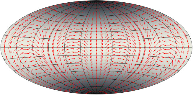
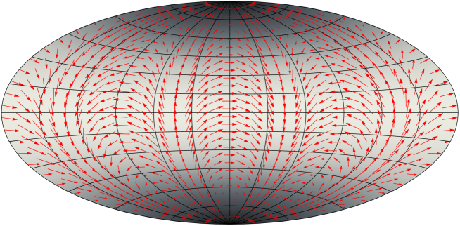
Figure 1: Vector fields $\delta^{i}_{+}$ (upper pane) and $\delta^{i}_{\times}$ (lower pane) for a gravitational wave propagating towards the north pole $\delta_{\rm gw}=\pi/2$. The maps use an Aitoff projection in equatorial coordinates $(\alpha,\delta)$, with origin $\alpha=\delta=0$ at the centre and $\alpha$ increasing from right to left. The gray-scale in the background shows the magnitude of the vector field (the lighter the bigger), which is equal to $\frac{1}{2}\,\cos\delta$ in both cases.

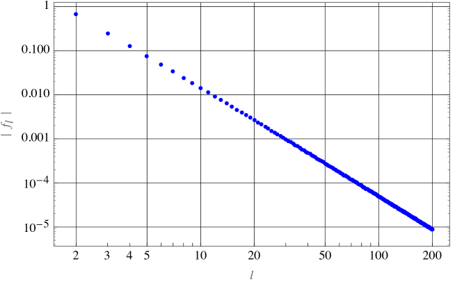
Figure 2: The absolute values of the coefficients $f_{l}$. The values of $f_{l}$ are related to the relative amplitudes of the astrometric signal from a gravitational wave at different VSH orders as given by Eqs. (56)–(57) and are more relevant for astrometric detection than the values of $g_{l}$ shown on Fig. 1 of (Book & Flanagan, 2011).

Having the observational data for ${\bf V}_{c}$ and ${\bf V}_{s}$ for certain locations on the sky (see Section V), one can fit the coefficients $t_{lm}$ and $s_{lm}$ using a sort of least squares estimator. Many details of this procedure is given in e.g. Section 5 of (Mignard & Klioner, 2012). In this way for a given frequency $\nu$ one gets two sets of the coefficients $(t^{c}_{lm},s^{c}_{lm})$ and $(t^{s}_{lm},s^{s}_{lm})$ for ${\bf V}_{c}$ and ${\bf V}_{s}$, respectively. These sets of coefficients can be used to decide if a signal from a gravitational wave is detected in the data (see again Section 5 of (Mignard & Klioner, 2012)). In addition to the standard statistical criteria, the symmetries of the signal and in particular the fact that the power is equal in the toroidal and spheroidal harmonics at each order as well as the decrease of the power with $l$ given by (61) can be used to distinguish the signal due to gravitational waves from other kinds of signals. If a signal is detected for some frequency $\nu$ the VSH coefficients can be converted back to the 6 parameters $h^{+}_{c}$, $h^{+}_{s}$, $h^{\times}_{c}$ and $h^{\times}_{s}$, $\alpha_{\rm gw}$, and $\delta_{\rm gw}$ using the model above and the transformation laws of the coefficients under rotations as described e.g. in (Mignard & Klioner, 2012, Section 3). To increase the signal-to-noise ratio when computing $(\alpha_{\rm gw},\delta_{\rm gw})$ one can also analyze the formal sum ${\bf V}_{c}+{\bf V}_{s}$. As discussed in Section V these estimated values of the gravitational wave parameters should be used for a final fit of those parameters directly in the astrometric solution.

VII Possible frequency limits and sensitivity of Gaia astrometry

The frequency $\nu$ of the signal that can be potentially detected by Gaia is not arbitrary. The upper limit for $\nu$ comes from the fact that the Gaia instrument should be calibrated from the same data. Although the details of the calibration are not fully known it is likely that the calibration will attempt to eliminate all periodic signals in the data with periods smaller than 1.5–2 rotational periods. Considering the best case one concludes that $\nu\leq 3\times 10^{-5}$ Hz. The lower limit for $\nu$ is related to the fact that the slow variations of position are well represented by proper motions – the first regime discussed in Section II. In the second regime, which we consider now, the period of gravitational waves should be (much) smaller than the time span of observations. Again considering the the best case and the planned mission duration of 5 yr one gets $\nu\geq 6.4\times 10^{-9}$ Hz. Finally, one gets

$$6.4\times 10^{-9}\ {\rm Hz}\leq\nu\leq 3\times 10^{-5}\,{\rm Hz}\,.$$ (62)

We note here that the lower limit for the frequency can be better (lower) in reality since the regimes discussed in Section II don’t have strict boundaries. It is clear that if the period of the gravitational wave is exactly equal to the time span of observations the astrometric solution is unable to adsorb the corresponding astrometric signal by proper motions which are linear in time. This is the third regime mentioned in Section II. Therefore, one can expect that the lower limit for the frequency can be lowered to about $3\times 10^{-9}$ Hz.

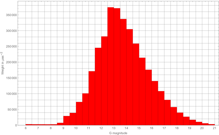
Figure 3: The distribution of the statistical weight of Gaia observations as function of Gaia magnitude $G$. Each bin shows the statistical weight of observations of sources in the corresponding interval of G. Here the post-launch estimates of the errors of Gaia observations were used. A version of this figure for the pre-launch error estimates and for only 10% of sources can be seen as Fig. 2 of (Hobbs et al., 2010).

Another goal of this Section is to discuss the sensitivity that can be expected from Gaia data. The expected astrometric accuracy of Gaia observations can be found at http://www.cosmos.esa.int/web/gaia/science-performance#astrometric%20performance. This accuracy can be converted to the expected uncertainties of a single observation of Gaia as function of the Gaia magnitude $G$ as defined (Jordi et al., 2010). Then a model of the Universe (Robin et al., 2012) can be used to compute the number of sources expected in each small interval in $G$. Combining the uncertainties of observations with the star counts one can calculate that the total statistical weight of all Gaia observations for stars up to magnitude $G=20$ reads (Klioner & Steidelmüller, 2012; Klioner, 2015)

$$W_{\rm full}=3.4\times 10^{6}\,{\hbox{\rm$\mu$as}}^{-2}\,.$$ (63)

Fig. 3 shows the distribution of the statistical weights of observations in certain intervals in $G$. One can see that sources with $12\leq G\leq 15$ are the most important for the determination. As with other global parameters in Gaia (e.g. the PPN $\gamma$) one can come to the idea to use only bright stars with, say, $G\leq 16$. This would considerably reduce the amount of observations (one can expect about $10^{8}$ such sources) while almost retaining the final accuracy of determination: $W_{\rm full}^{G\leq 16}=3.0\times 10^{6}\,{\hbox{\rm$\mu$as}}^{-2}$. However, such a selection of source is dangerous in the presence of calibration errors that are often strongly depend on the magnitude and related parameters. The idea to compute normal points presented above makes such a selection unnecessary.

We are interested in sensitivity of Gaia data to the overall amplitude of the gravitational wave $h=\sqrt{\left(h^{+}_{c}\right)^{2}+\left(h^{+}_{s}\right)^{2}+\left(h^{\times}_{c}\right)^{2}+\left(h^{\times}_{s}\right)^{2}}$. For any scalar parameter $h$ to be fitted to the Gaia data, the maximal possible accuracy of its determination is $\left(W_{\rm full}\right)^{-1/2}$. This lower estimate holds if the partial derivatives with respect to the parameter are equal to unity for all observations. Therefore,

$$\sigma_{h}\geq\left(W_{\rm full}\right)^{-1/2}=5.4\times 10^{-4}\,\hbox{\rm$\mu$as}=2.6\times 10^{-15}\,.$$ (64)

Obviously, the actual sensitivity will be lower because of various correlations and systematic errors. One can write

$$\sigma_{h}\approx 2.6\times 10^{-15}\,Q\,,$$ (65)

where $Q$ is a numerical factor depending on the details of Gaia observations. As a plain guess it is reasonable to assume that $Q\sim 10-1000$. This factor reflects the fact that the same observation are used to fit the source, attitude and calibration parameters (see Section I) as well as some systematic errors. Note, however, that this should not be interpreted as a claim of real sensitivity of Gaia. This only gives an estimate of the best possible sensitivity.

The actual sensitivity curve (including the actual frequency limits) should be determined by detailed end-to-end numerical simulations involving in particular the interaction between the astrometric signal of a gravitational wave and the standard astrometric solution. The results of these simulations will be the subject of a separate publication.

VIII Sources of gravitational waves for space astrometry

It is clear that the most promising sources of gravitational waves for astrometric detection are supermassive binary black holes in the centres of galaxies. Recently, such systems were often discussed in the literature (see, e.g., (Yonemaru et.al., 2016; Graham et al., 2015a, b; Merritt, 2017)). It is believed that binary supermassive black holes are a relatively common product of interaction and merging of galaxies in the typical course of their evolution. This sort of objects can give gravitational waves with both frequencies and amplitudes potentially within the reach of space astrometry. Moreover, the gravitational waves from those objects can often be considered to have virtually constant frequency and amplitude during the whole period of observations of several years. A binary system with a chirp mass ${\cal M}$ on a circular orbit with the orbital period $P$ emits gravitational waves of the period $P_{\rm gw}=P/2$ and strain (Jaranowski & Królak, 2009; Buonanno, 2007)

$$h = {4\,\pi^{2/3}\over c^{4}}\,{\left(G{\cal M}\right)}^{5/3}\,P_{\rm gw}^{-2/3}\,r^{-1}$$ (66)

$$= 1.19\times 10^{-14}\,\left({{\cal M}\over 10^{9}\,M_{\odot}}\right)^{5/3}\,\left({P_{\rm gw}\over 1\ {\rm yr}}\right)^{-2/3}\,\left({r\over 100\ {\rm Mpc}}\right)^{-1}\,,$$

where $r$ is the (luminosity) distance to the source, $G$ is the Newtonian constant of gravitation, and $M_{\odot}$ is the Solar mass. This equation gives the strain for both polarizations in the direction perpendicular to the orbital plane. Two polarizations have different dependence on the inclination of the orbit (Jaranowski & Królak, 2009). For eccentric orbits the strain is moderately increased approximately as $h\propto(1-e^{2})^{-1}$. However, eccentricity of the orbit is not expected to play a big role since eccentricity decreases during the evolution and one should generally expect small eccentricities. The above estimate is derived in the linear approximation of general relativity, which means that it is valid when

$$P_{\rm gw}\gg 10^{\rm h}\,\left({{\cal M}\over 10^{9}\,M_{\odot}}\right)\,.$$ (67)

This is the condition that the semi-major axis of the orbit is much larger than the sum of the Schwarzschild radii of the components. It is well known that such a massive binary system loses energy due to gravitational radiation, so that its orbital period decreases (inspiralling orbit) and the frequency of gravitational wave $\nu_{\rm gw}=1/P_{\rm gw}$ increases. The derivative $\dot{\nu}_{\rm gw}$ can be computed from the energy balance between the emitted gravitational waves and the orbital motion (Jaranowski & Królak, 2009; Buonanno, 2007):

$$\dot{\nu}_{\rm gw}={96\over 5}\pi^{8/3}\,{\left({G{\cal M}\over c^{3}}\right)}^{5/3}\,\nu_{\rm gw}^{11/3}=5.83\times 10^{-12}\ {\rm Hz/yr}\,\left({{\cal M}\over 10^{9}\,M_{\odot}}\right)^{5/3}\,\left({P_{\rm gw}\over 1\ {\rm yr}}\right)^{-11/3}\,.$$ (68)

Integrating this equation one gets that the time to coalescence $\tau=t_{\rm coal}-t_{\rm obs}$ (in this approximation $\nu_{\rm gw}$ goes to infinity at the coalescence) reads (Jaranowski & Królak, 2009; Buonanno, 2007):

$$\tau = {3\over 8}\,{\nu_{\rm gw}\over\dot{\nu}_{\rm gw}}={5\over 256}\,\pi^{-8/3}\,{\left({G{\cal M}\over c^{3}}\right)}^{-5/3}\,P_{\rm gw}^{8/3}=2039\ {\rm yr}\,\left({{\cal M}\over 10^{9}\,M_{\odot}}\right)^{-5/3}\,\left({P_{\rm gw}\over 1\ {\rm yr}}\right)^{8/3}\,.$$ (69)

Here $\nu_{\rm gw}$, $\dot{\nu}_{\rm gw}$ and $P_{\rm gw}$ are evaluated at the moment of observation $t_{\rm obs}$. Eqs. (66) and (69) give a useful insight of what sort of binary systems can be within the reach of space astrometry: the strain (66) should be large (say, $\gtrsim 10^{-13}$ for Gaia) and the time to coalescence should be large enough to guarantee almost constant frequency of gravitational wave during the whole period of observations (of 5–10 years for Gaia).

It is clear that the known candidates for binary supermassive black holes are rather speculative. Nevertheless, it seems to be useful to give estimates of the expected strain of the gravitational waves from those sources. Substituting the corresponding parameters of the candidates (Valtonen et al., 2016; Graham et al., 2015a; Yonemaru et.al., 2016) into the formulas above one gets strains of about $h\sim 2\times 10^{-16}$ with a period of 6 yr for OJ287 assuming the chirp mass of $8\times 10^{8}\,M_{\odot}$, $h\lesssim 5\times 10^{-16}$ with a period of 2.6 yr for PG 1302–102, and $h<1.3\times 10^{-12}\,\left(P/\,1\,{\rm yr}\right)^{-2/3}$ for M87 assuming equal mass components. Although we cannot identify promising sources of gravitational waves for Gaia astrometry now, it is important to note that $h$ is proportional to ${\cal M}^{5/3}/r$ so that moderate increase in the chirp mass can compensate greater distances. Currently one suspects supermassive black holes with masses $>10^{10}\,M_{\odot}$ in a number of galaxies. Some of them may turn out to be binary systems and represent sources of gravitational waves for high-accuracy astrometry.

IX Concluding remarks

In this report we summarized the model for astrometric effects of a plane gravitational wave with constant frequency. The model and the most important partial derivatives are given by Eqs. (3)–(22) and (25)–(34).

The search algorithm based on the data normal points and VSH analysis described in Sections V and VI is very promising to reduce the computational complexity of the search for gravitational waves in the observational data especially in combination with the HEALPix pixelization (Górsky et al., 2005).

In Section VII we gave estimates for the frequency range in which a Gaia-like instrument can be used to detect gravitational waves as periodic deflection signals. We also gave an estimate for the best-case sensitivity of Gaia astrometry. An overview of the main characteristics of gravitational waves from the binary supermassive black holes, which obviously represent the most promising astrophysical sources for space astrometry, is given in Section VIII.

The simplest version of the gravitational wave model discussed above is to assume that the frequency $\nu$ is constant. In principle, it is straightforward to accommodate the search algorithm to the case when the frequency is a given function of time as e.g. in Eq. (68). It is sufficient to use this function in (39) when computing vector fields ${\bf V}_{c}$ and ${\bf V}_{s}$ using (38) or (40). Obviously one should also accommodate the time-dependence of the strain parameters: ${\bf V}_{c}$ and ${\bf V}_{s}$ are no longer time independent in this case. Since astrometry is most sensitive to gravitational waves of almost constant frequency and strain, the time dependence of parameters can be sufficiently approximated by a linear functions of time. This generalization is possible, however would increase the number of parameters to be fitted.

Another important aspect is the situation when several gravitational waves of comparable amplitudes from different sources are superimposed. In principle, if a number of strong signals have different frequencies (which is physically almost guaranteed) no modification of the algorithm is needed: the signals will be found one by one. On the other hand, in the highly unlikely case of two gravitational waves with equal frequencies coming from different sources it is difficult to separate them since the sum of two different quadrupole signals on the sky is equivalent to another one quadrupole signal with certain parameters. It is, however, doubtful that this regime is of any practical interest, except for the case of stochastic background of gravitational waves. The latter case is beyond the scope of this work.

The search and fit algorithms sketched in Sections V and VI are being further developed and implemented to work with the real Gaia data in the framework of Gaia Data Processing and Analysis Consortium (Gaia DPAC). Further details will be published elsewhere.