A Neural-Symbolic Approach to Design of CAPTCHA

Abstract

CAPTCHAs based on reading text are susceptible to machine-learning-based attacks [1] due to recent significant advances in deep learning (DL). To address this, this paper promotes image/visual captioning based CAPTCHAs, which is robust against machine-learning-based attacks. To develop image/visual-captioning-based CAPTCHAs, this paper proposes a new image captioning architecture by exploiting tensor product representations (TPR), a structured neural-symbolic framework developed in cognitive science over the past 20 years, with the aim of integrating DL with explicit language structures and rules. We call it the Tensor Product Generation Network (TPGN). The key ideas of TPGN are: 1) unsupervised learning of role-unbinding vectors of words via a TPR-based deep neural network, and 2) integration of TPR with typical DL architectures including Long Short-Term Memory (LSTM) models. The novelty of our approach lies in its ability to generate a sentence and extract partial grammatical structure of the sentence by using role-unbinding vectors, which are obtained in an unsupervised manner. Experimental results demonstrate the effectiveness of the proposed approach.

1 Introduction

CAPTCHA, which stands for “Completely Automated Public Turing test to tell Computers and Humans Apart”, is a type of challenge-response test used in computers to determine whether or not the user is a human [1]. Most CAPTCHA systems are based on reading text contained in an image as shown in Fig. 1. However, such systems can be easily cracked by deep learning since deep learning can achieve very high accuracy in recognizing text. To address this, this paper proposes a new CAPTCHA, which distinguishes a human from a computer by testing the capability of image captioning (which generates a caption for a given image) or video storytelling (which generates a story consisting of multiple sentences for a give video sequence). It is known that the performance of computerized image captioning or video storytelling is far from human performance [2]. Hence, image/visual captioning based CAPTCHAs can more reliably distinguish computers from humans.

Figure 1: Reading-text-based CAPTCHA.

Deep learning is an important tool in many current natural language processing (NLP) applications. However, language rules or structures cannot be explicitly represented in deep learning architectures. The tensor product representation developed in [3, 4] has the potential of integrating deep learning with explicit rules (such as logical rules, grammar rules, or rules that summarize real-world knowledge). This paper develops a TPR approach for image/visual-captioning-based CAPTCHAs, introducing the Tensor Product Generation Network (TPGN) architecture.

A TPGN model generates natural language descriptions via learned representations. The representations learned in a crucial layer of the TPGN can be interpreted as encoding grammatical roles for the words being generated. This layer corresponds to the role-encoding component of a general, independently-developed architecture for neural computation of symbolic functions, including the generation of linguistic structures. The key to this architecture is the notion of Tensor Product Representation (TPR), in which vectors embedding symbols (e.g., lives, frodo) are bound to vectors embedding structural roles (e.g., verb, subject) and combined to generate vectors embedding symbol structures ([frodo lives]). TPRs provide the representational foundations for a general computational architecture called Gradient Symbolic Computation (GSC), and applying GSC to the task of natural language generation yields the specialized architecture defining the model presented here. The generality of GSC means that the results reported here have implications well beyond the particular task we address here.

In our proposed image/visual captioning based CAPTCHA, a TPGN takes an image ${\mathbf{I}}$ as input and generates a caption. Then, an evaluator will evaluate the TPGN’s captioning performance by calculating the metric of SPICE [5] by comparing to human-generated gold-standard captions. If the SPICE value is less than a threshold, this input image ${\mathbf{I}}$ can be used as a challenge in our CAPTCHA. In this way, we can obtain a set ${\mathbf{B}}$ of images to be used as challenges in CAPTCHA.

In our CAPTCHA shown in Fig. 2, an image is randomly selected from the set ${\mathbf{B}}$ and rendered as a challenge; a tester is asked to give a description of the image as an answer. An evaluator calculates a SPICE value for the answer. If the SPICE value is greater than a threshold, the answer is considered to be correct and the tester is deemed to be a human; otherwise, the tester is deemed to be a computer.

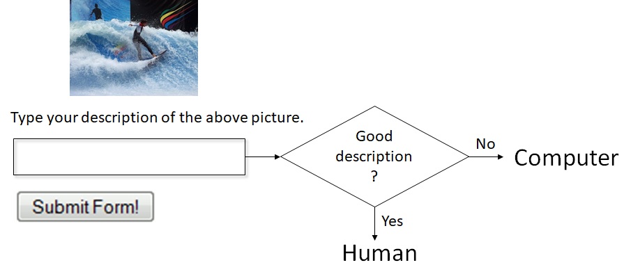
Figure 2: Image-captioning-based CAPTCHA.

The paper is organized as follows. Section 2 presents the rationale for our proposed architecture. In Section 3, we present our experimental results. Finally, Section 4 concludes the paper.

Figure 3: Architecture of TPGN, a TPR-capable generation network. “$\Box\times$” denotes the matrix-vector product.

2 Design of image-captioning-based CAPTCHA

2.1 A TPR-capable generation architecture

In this work we propose an approach to network architecture design we call the TPR-capable method. The architecture we use (see Fig. 3) is designed so that TPRs could, in theory, be used within the architecture to perform the target task — here, generating a caption one word at a time. Unlike previous work where TPRs are hand-crafted, in our work, end-to-end deep learning will induce representations which the architecture can use to generate captions effectively.

As shown in Fig. 3, our proposed system is denoted by $\mathcal{N}$. The input of $\mathcal{N}$ is an image feature vector $\mathbf{v}$ and the output of $\mathcal{N}$ is a caption. The image feature vector $\mathbf{v}$ is extracted from a given image by a pre-trained CNN. The first part of our system $\mathcal{N}$ is a sentence-encoding subnetwork $\mathcal{S}$ which maps $\mathbf{v}$ to a representation $S$ which will drive the entire caption-generation process; $S$ contains all the image-specific information for producing the caption. (We will call a caption a “sentence” even though it may in fact be just a noun phrase.)

If $S$ were a TPR of the caption itself, it would be a matrix (or 2-index tensor) $\mathbf{S}$ which is a sum of matrices, each of which encodes the binding of one word to its role in the sentence constituting the caption. To serially read out the words encoded in $\mathbf{S}$, in iteration 1 we would unbind the first word from $\mathbf{S}$, then in iteration 2 the second, and so on. As each word is generated, $\mathbf{S}$ could update itself, for example, by subtracting out the contribution made to it by the word just generated; $\mathbf{S}_{t}$ denotes the value of $\mathbf{S}$ when word $w_{t}$ is generated. At time step $t$ we would unbind the role $r_{t}$ occupied by word $w_{t}$ of the caption. So the second part of our system $\mathcal{N}$ — the unbinding subnetwork $\mathcal{U}$ — would generate, at iteration $t$, the unbinding vector $\mathbf{u}_{t}$. Once $\mathcal{U}$ produces the unbinding vector $\mathbf{u}_{t}$, this vector would then be applied to $\mathbf{S}$ to extract the symbol $\bf{f}_{t}$ that occupies word $t$’s role; the symbol represented by $\bf{f}_{t}$ would then be decoded into word $w_{t}$ by the third part of $\mathcal{N}$, i.e., the lexical decoding subnetwork $\mathcal{L}$, which outputs $\mathbf{x}_{t}$, the 1-hot-vector encoding of $w_{t}$.

Unbinding in TPR is achieved by the matrix-vector product (see Appendix A). So the key operation in generating $w_{t}$ is thus the unbinding of $r_{t}$ within $\mathbf{S}$, which amounts to simply:

$$\mathbf{S}_{t}\bf{u}_{t}=\bf{f}_{t}.$$ (1)

This matrix-vector product is denoted “$\Box\times$” in Fig. 3.

Thus the system $\mathcal{N}$ of Fig. 3 is TPR-capable. This is what we propose as the Tensor-Product Generation Network (TPGN) architecture. The learned representation $\mathbf{S}$ will not be proven to literally be a TPR, but by analyzing the unbinding vectors $\mathbf{u}_{t}$ the network learns, we will gain insight into the process by which the learned matrix $\mathbf{S}$ gives rise to the generated caption.

What type of roles might the unbinding vectors be unbinding? A TPR for a caption could in principle be built upon positional roles, syntactic/semantic roles, or some combination of the two. In the caption a man standing in a room with a suitcase, the initial a and man might respectively occupy the positional roles of $\textsc{pos(ition)}_{1}$ and $\textsc{pos}_{2}$; standing might occupy the syntactic role of verb; in the role of Spatial-P(reposition); while a room with a suitcase might fill a 5-role schema $\textsc{Det(erminer)}_{1}\textsc{ N(oun)}_{1}\textsc{ P Det}_{2}\textsc{ N}_{2}$. In fact, there is evidence that our network learns just this kind of hybrid role decomposition.

What form of information does the sentence-encoding subnetwork $\mathcal{S}$ need to encode in $\mathbf{S}$? Continuing with the example of the previous paragraph, $\mathbf{S}$ needs to be some approximation to the TPR summing several filler/role binding matrices. In one of these bindings, a filler vector $\mathbf{f}_{\textit{a}}$ — which the lexical subnetwork $\mathcal{L}$ will map to the article a — is bound (via the outer product) to a role vector $\mathbf{r}_{\textsc{Pos}_{1}}$ which is the dual of the first unbinding vector produced by the unbinding subnetwork $\mathcal{U}$: $\mathbf{u}_{\textsc{Pos}_{1}}$. In the first iteration of generation the model computes $\mathbf{S}_{1}\mathbf{u}_{\textsc{Pos}_{1}}=\mathbf{f}_{\textit{a}}$, which $\mathcal{L}$ then maps to a. Analogously, another binding approximately contained in $\mathbf{S}_{2}$ is $\mathbf{f}_{\textit{man}}\mathbf{r}_{\textsc{Pos}_{2}}^{\top}$. There are corresponding bindings for the remaining words of the caption; these employ syntactic/semantic roles. One example is $\mathbf{f}_{\textit{standing}}\mathbf{r}_{V}^{\top}$. At iteration 3, $\mathcal{U}$ decides the next word should be a verb, so it generates the unbinding vector $\mathbf{u}_{V}$ which when multiplied by the current output of $\mathcal{S}$, the matrix $\mathbf{S}_{3}$, yields a filler vector $\mathbf{f}_{\textit{standing}}$ which $\mathcal{L}$ maps to the output standing. $\mathcal{S}$ decided the caption should deploy standing as a verb and included in $\mathbf{S}$ the binding $\mathbf{f}_{\textit{standing}}\mathbf{r}_{V}^{\top}$. It similarly decided the caption should deploy in as a spatial preposition, including in $\mathbf{S}$ the binding $\mathbf{f}_{\textit{in}}\mathbf{r}_{\textsc{Spatial-P}}^{\top}$; and so on for the other words in their respective roles in the caption.

2.2 CAPTCHA generation method

We first describe how to obtain a set of images as challenges in our CAPTCHA system. In our proposed image/visual captioning based CAPTCHA, a TPGN takes an image ${\mathbf{I}}$ as input and generates a caption. Then, an evaluator will evaluate the TPGN’s captioning performance by calculating the metric of SPICE [5] by comparing to human-generated gold-standard captions. If the SPICE value is less than a threshold $\gamma_{1}$, this input image ${\mathbf{I}}$ can be used as a challenge in our CAPTCHA; otherwise, this input image ${\mathbf{I}}$ will not be selected as a challenge and a new image will be examined. In this way, we can obtain a set ${\mathbf{B}}$ of images used as challenges in CAPTCHA. All images in ${\mathbf{B}}$ are difficult to be captioned by a computerized image captioning system due to their low SPICE values.

Now, we describe our CAPTCHA generation method. In our CAPTCHA, an image is randomly selected from the set ${\mathbf{B}}$ and rendered as a challenge; a tester is asked to give a description of the image as an answer. An evaluator calculates a SPICE value for the answer. If the SPICE value is greater than a threshold $\gamma_{2}$, the answer is considered to be correct and the tester is deemed to be a human; otherwise, the answer is considered to be wrong and the tester is deemed to be a computer.

Due to space limitations, the detailed design of our system is described in Appendix B; and TPR is reviewed in Appendix A.

3 Experimental results

To evaluate the performance of our proposed architecture, we use the COCO dataset [2]. The COCO dataset contains 123,287 images, each of which is annotated with at least 5 captions. We use the same pre-defined splits as [6, 7]: 113,287 images for training, 5,000 images for validation, and 5,000 images for testing. We use the same vocabulary as that employed in [7], which consists of 8,791 words.

For the CNN of Fig. 3, we used ResNet-152 [8], pretrained on the ImageNet dataset. The feature vector ${\mathbf{v}}$ has 2048 dimensions. Word embedding vectors in ${\mathbf{W}}_{e}$ are downloaded from the web [9]. The model is implemented in TensorFlow [10] with the default settings for random initialization and optimization by backpropagation.

In our experiments, we choose $d=25$ (where $d$ is the dimension of vector ${\mathbf{p}}_{t}$). The dimension of ${\mathbf{S}}_{t}$ is $625\times 625$; the vocabulary size $V=8,791$; the dimension of ${\mathbf{u}}_{t}$ and ${\mathbf{f}}_{t}$ is $d^{2}=625$.

Table 1: Performance of the proposed TPGN model on the COCO dataset.

Methods	METEOR	BLEU-1	BLEU-2	BLEU-3	BLEU-4	CIDEr	SPICE
NIC [11]	–	0.666	0.451	0.304	0.203	–	–
CNN-LSTM	0.238	0.698	0.525	0.390	0.292	0.889	–
TPGN	0.243	0.709	0.539	0.406	0.305	0.909	0.18

The main evaluation results on the MS COCO dataset are reported in Table 1. The widely-used BLEU [12], METEOR [13], CIDEr [14], and SPICE [5] metrics are reported in our quantitative evaluation of the performance of the proposed schemes. In evaluation, our baseline is the widely used CNN-LSTM captioning method originally proposed in [11]. For comparison, we include results in that paper in the first line of Table 1. We also re-implemented the model using the latest ResNet feature and report the results in the second line of Table 1. Our re-implementation of the CNN-LSTM method matches the performance reported in [7], showing that the baseline is a state-of-the-art implementation. As shown in Table 1, compared to the CNN-LSTM baseline, the proposed TPGN significantly outperforms the benchmark schemes in all metrics across the board. The improvement in BLEU-$n$ is greater for greater $n$; TPGN particularly improves generation of longer subsequences. The results clearly attest to the effectiveness of the TPGN architecture.

Now, we address the issue of how to determine the two thresholds $\gamma_{1}$ and $\gamma_{2}$ in our CAPTCHA system. We set $\gamma_{1}=0.04$, which is about 80% less than the SPICE metric obtained by TPGN. In this way, the image set ${\mathbf{B}}$ only contains images that are most difficult to be captioned by a computer.

We run a trained TPGN with input images from COCO test dataset, and select ten images from COCO test dataset, whose SPICE metrics are less than $\gamma_{1}$. Then we use Amazon Mechanical Turk system to generate captions for these ten images by humans. We observe that the SPICE metric obtained by a caption generated by a human is always larger than 0.3; hence, we set $\gamma_{2}=0.3$, which is much larger than the SPICE metric achievable by any existing computerized image captioning system [2].

4 Conclusion

In this paper, we proposed a new Tensor Product Generation Network (TPGN) for image/visual-captioning-based CAPTCHAs. The model has a novel architecture based on a rationale derived from the use of Tensor Product Representations for encoding and processing symbolic structure through neural network computation. In evaluation, we tested the proposed model on captioning with the MS COCO dataset, a large-scale image-captioning benchmark. Compared to widely adopted LSTM-based models, the proposed TPGN gives significant improvements on all major metrics including METEOR, BLEU, CIDEr, and SPICE. Our findings in this paper show great promise of TPRs in CAPTCHA. In the future, we will explore extending TPR to a variety of other NLP tasks and spam email detection.

Appendix

Appendix A Review of tensor product representation

Tensor product representation (TPR) is a general framework for embedding a space of symbol structures $\mathfrak{S}$ into a vector space. This embedding enables neural network operations to perform symbolic computation, including computations that provide considerable power to symbolic NLP systems [4, 15]. Motivated by these successful examples, we are inspired to extend the TPR to the challenging task of learning image captioning. And as a by-product, the symbolic character of TPRs makes them amenable to conceptual interpretation in a way that standard learned neural network representations are not.

A particular TPR embedding is based in a filler/role decomposition of $\mathfrak{S}$ . A relevant example is when $\mathfrak{S}$ is the set of strings over an alphabet $\{\mathtt{a},\mathtt{b},\ldots\}$. One filler/role decomposition deploys the positional roles $\{r_{k}\},k\in\mathbb{N}$, where the filler/role binding $\mathtt{a}/r_{k}$ assigns the ‘filler’ (symbol) $\mathtt{a}$ to the $k^{th}$ position in the string. A string such as $\mathtt{abc}$ is uniquely determined by its filler/role bindings, which comprise the (unordered) set $\mathfrak{B}(\mathtt{abc})=\{\mathtt{b}/r_{2},\mathtt{a}/r_{1},\mathtt{c}/r_{3}\}$. Reifying the notion role in this way is key to TPR’s ability to encode complex symbol structures.

Given a selected filler/role decomposition of the symbol space, a particular TPR is determined by an embedding that assigns to each filler a vector in a vector space $V_{F}\cong\mathbb{R}^{d_{F}}$, and a second embedding that assigns to each role a vector in a space $V_{R}\cong\mathbb{R}^{d_{R}}$. The vector embedding a symbol $\mathtt{a}$ is denoted by $\mathbf{f_{\mathtt{a}}}$ and is called a filler vector; the vector embedding a role $r_{k}$ is $\mathbf{r_{k}}$ and called a role vector. The TPR for $\mathtt{abc}$ is then the following 2-index tensor in $V_{F}\otimes V_{R}\cong\mathbb{R}^{d_{F}\times d_{R}}$:

$$\bf{S}_{\mathtt{\mathtt{abc}}}=\mathbf{f_{\mathtt{b}}}\otimes\mathbf{r_{2}}+\mathbf{f_{\mathtt{a}}}\otimes\mathbf{r_{1}}+\mathbf{f_{\mathtt{c}}}\otimes\mathbf{r_{3}},$$ (2)

where $\otimes$ denotes the tensor product. The tensor product is a generalization of the vector outer product that is recursive; recursion is exploited in TPRs for, e.g., the distributed representation of trees, the neural encoding of formal grammars in connection weights, and the theory of neural computation of recursive symbolic functions. Here, however, it suffices to use the outer product; using matrix notation we can write (2) as:

$$\bf{S}_{\mathtt{abc}}=\mathbf{f_{\mathtt{b}}}\mathbf{r_{2}}^{\!\!\top}+\mathbf{f_{\mathtt{a}}}\mathbf{r_{1}}^{\!\!\top}+\mathbf{f_{\mathtt{c}}}\mathbf{r_{3}}^{\!\!\top}.$$ (3)

Generally, the embedding of any symbol structure $\mathtt{S}\in\mathfrak{S}$ is $\sum\{\mathbf{f}_{i}\otimes\mathbf{r}_{i}\mid\mathtt{f}_{i}/r_{i}\in\mathfrak{B}(\mathtt{S})\}$; here: $\sum\{\mathbf{f}_{i}\mathbf{r}_{i}^{\top}\mid\mathtt{f}_{i}/r_{i}\in\mathfrak{B}(\mathtt{S})\}$ [3, 4].

A key operation on TPRs, central to the work presented here, is unbinding, which undoes binding. Given the TPR in (3), for example, we can unbind $\mathbf{r_{2}}$ to get $\mathbf{f_{\mathtt{b}}}$; this is achieved simply by $\mathbf{f_{\mathtt{b}}}=\mathbf{S_{\mathtt{abc}}}\mathbf{u_{2}}$. Here $\mathbf{u_{2}}$ is the unbinding vector dual to the binding vector $\mathbf{r_{2}}$. To make such exact unbinding possible, the role vectors should be chosen to be linearly independent. (In that case the unbinding vectors are the rows of the inverse of the matrix containing the binding vectors as columns, so that $\mathbf{r_{2}\cdot u_{2}}=1$ while $\mathbf{r_{k}\cdot u_{2}}=0$ for all other role vectors $\mathbf{r_{k}\neq r_{2}}$; this entails that $\mathbf{S_{\mathtt{abc}}}\mathbf{u_{2}}=\mathbf{b}$, the filler vector bound to $\mathbf{r_{2}}$. Replacing the matrix inverse with the pseudo-inverse allows approximate unbinding when the role vectors are not linearly independent).

Appendix B System Description

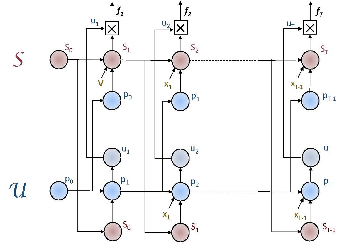
Figure 4: The sentence-encoding subnet $\mathcal{S}$ and the unbinding subnet $\mathcal{U}$ are inter-connected LSTMs; $\mathbf{v}$ encodes the visual input while the $\mathbf{x}_{t}$ encode the words of the output caption.

The unbinding subnetwork $\mathcal{U}$ and the sentence-encoding network $\mathcal{S}$ of Fig. 3 are each implemented as (1-layer, 1-directional) LSTMs (see Fig. 4); the lexical subnetwork $\mathcal{L}$ is implemented as a linear transformation followed by a softmax operation. In the equations below, the LSTM variables internal to the $\mathcal{S}$ subnet are indexed by 1 (e.g., the forget-, input-, and output-gates are respectively $\mathbf{\hat{f}}_{1},\mathbf{\hat{i}}_{1},\mathbf{\hat{o}}_{1}$) while those of the unbinding subnet $\mathcal{U}$ are indexed by 2.

Thus the state updating equations for $\mathcal{S}$ are, for $t=1,\cdots,T$ = caption length:

$${\mathbf{\hat{f}}}_{1,t} = \sigma_{g}({\mathbf{W}}_{1,f}{\mathbf{p}}_{t-1}-{\mathbf{D}}_{1,f}{\mathbf{W}}_{e}{\mathbf{x}}_{t-1}+{\mathbf{U}}_{1,f}{\mathbf{\hat{S}}}_{t-1})$$ (4)

$${\mathbf{\hat{i}}}_{1,t} = \sigma_{g}({\mathbf{W}}_{1,i}{\mathbf{p}}_{t-1}-{\mathbf{D}}_{1,i}{\mathbf{W}}_{e}{\mathbf{x}}_{t-1}+{\mathbf{U}}_{1,i}{\mathbf{\hat{S}}}_{t-1})$$ (5)

$${\mathbf{\hat{o}}}_{1,t} = \sigma_{g}({\mathbf{W}}_{1,o}{\mathbf{p}}_{t-1}-{\mathbf{D}}_{1,o}{\mathbf{W}}_{e}{\mathbf{x}}_{t-1}+{\mathbf{U}}_{1,o}{\mathbf{\hat{S}}}_{t-1})$$ (6)

$${\mathbf{g}}_{1,t} = \sigma_{h}({\mathbf{W}}_{1,c}{\mathbf{p}}_{t-1}-{\mathbf{D}}_{1,c}{\mathbf{W}}_{e}{\mathbf{x}}_{t-1}+{\mathbf{U}}_{1,c}{\mathbf{\hat{S}}}_{t-1})$$ (7)

$${\mathbf{c}}_{1,t} = {\mathbf{\hat{f}}}_{1,t}\odot{\mathbf{c}}_{1,t-1}+{\mathbf{\hat{i}}}_{1,t}\odot{\mathbf{g}}_{1,t}$$ (8)

$${\mathbf{\hat{S}}}_{t} = {\mathbf{\hat{o}}}_{1,t}\odot\sigma_{h}({\mathbf{c}}_{1,t})$$ (9)

where ${\mathbf{\hat{f}}}_{1,t}$, ${\mathbf{\hat{i}}}_{1,t}$, ${\mathbf{\hat{o}}}_{1,t}$, ${\mathbf{g}}_{1,t}$, ${\mathbf{c}}_{1,t}$, ${\mathbf{\hat{S}}}_{t}\in\mathbb{R}^{d\times d}$, ${\mathbf{p}}_{t}$ $\in\mathbb{R}^{d}$, $\sigma_{g}(\cdot)$ is the (element-wise) logistic sigmoid function; $\sigma_{h}(\cdot)$ is the hyperbolic tangent function; the operator $\odot$ denotes the Hadamard (element-wise) product; ${\mathbf{W}}_{1,f},{\mathbf{W}}_{1,i},{\mathbf{W}}_{1,o},{\mathbf{W}}_{1,c}\in\mathbb{R}^{d\times d\times d}$, ${\mathbf{D}}_{1,f}$, ${\mathbf{D}}_{1,i}$, ${\mathbf{D}}_{1,o}$, ${\mathbf{D}}_{1,c}$ $\in$ $\mathbb{R}^{d\times d\times d}$, ${\mathbf{U}}_{1,f}$, ${\mathbf{U}}_{1,i}$, ${\mathbf{U}}_{1,o}$, ${\mathbf{U}}_{1,c}$ $\in$ $\mathbb{R}^{d\times d\times d\times d}$. For clarity, biases — included throughout the model — are omitted from all equations in this paper. The initial state ${\mathbf{\hat{S}}}_{0}$ is initialized by:

$${\mathbf{\hat{S}}}_{0}={\mathbf{C}}_{s}({\mathbf{v}}-\bar{{\mathbf{v}}})$$ (10)

where ${\mathbf{v}}\in\mathbb{R}^{2048}$ is the vector of visual features extracted from the current image by ResNet [7] and $\bar{{\mathbf{v}}}$ is the mean of all such vectors; ${\mathbf{C}}_{s}\in\mathbb{R}^{d\times d\times 2048}$. On the output side, ${\mathbf{x}}_{t}\in\mathbb{R}^{V}$ is a 1-hot vector with dimension equal to the size of the caption vocabulary, $V$, and ${\mathbf{W}}_{e}\in\mathbb{R}^{d\times V}$ is a word embedding matrix, the $i$-th column of which is the embedding vector of the $i$-th word in the vocabulary; it is obtained by the Stanford GLoVe algorithm with zero mean [9]. ${\mathbf{x}}_{0}$ is initialized as the one-hot vector corresponding to a “start-of-sentence” symbol.

For $\mathcal{U}$ in Fig. 3, the state updating equations are:

$${\mathbf{\hat{f}}}_{2,t} = \sigma_{g}({\mathbf{\hat{S}}}_{t-1}{\mathbf{w}}_{2,f}-{\mathbf{D}}_{2,f}{\mathbf{W}}_{e}{\mathbf{x}}_{t-1}+{\mathbf{U}}_{2,f}{\mathbf{p}}_{t-1})$$ (11)

$${\mathbf{\hat{i}}}_{2,t} = \sigma_{g}({\mathbf{\hat{S}}}_{t-1}{\mathbf{w}}_{2,i}-{\mathbf{D}}_{2,i}{\mathbf{W}}_{e}{\mathbf{x}}_{t-1}+{\mathbf{U}}_{2,i}{\mathbf{p}}_{t-1})$$ (12)

$${\mathbf{\hat{o}}}_{2,t} = \sigma_{g}({\mathbf{\hat{S}}}_{t-1}{\mathbf{w}}_{2,o}-{\mathbf{D}}_{2,o}{\mathbf{W}}_{e}{\mathbf{x}}_{t-1}+{\mathbf{U}}_{2,o}{\mathbf{p}}_{t-1})$$ (13)

$${\mathbf{g}}_{2,t} = \sigma_{h}({\mathbf{\hat{S}}}_{t-1}{\mathbf{w}}_{2,c}-{\mathbf{D}}_{2,c}{\mathbf{W}}_{e}{\mathbf{x}}_{t-1}+{\mathbf{U}}_{2,c}{\mathbf{p}}_{t-1})$$ (14)

$${\mathbf{c}}_{2,t} = {\mathbf{\hat{f}}}_{2,t}\odot{\mathbf{c}}_{2,t-1}+{\mathbf{\hat{i}}}_{2,t}\odot{\mathbf{g}}_{2,t}$$ (15)

$${\mathbf{p}}_{t} = {\mathbf{\hat{o}}}_{2,t}\odot\sigma_{h}({\mathbf{c}}_{2,t})$$ (16)

where ${\mathbf{w}}_{2,f},{\mathbf{w}}_{2,i},{\mathbf{w}}_{2,o},{\mathbf{w}}_{2,c}\in\mathbb{R}^{d}$, ${\mathbf{D}}_{2,f},{\mathbf{D}}_{2,i},{\mathbf{D}}_{2,o},{\mathbf{D}}_{2,c}$ $\in$ $\mathbb{R}^{d\times d}$, and ${\mathbf{U}}_{2,f},{\mathbf{U}}_{2,i},{\mathbf{U}}_{2,o},{\mathbf{U}}_{2,c}$ $\in$ $\mathbb{R}^{d\times d}$. The initial state ${\mathbf{p}}_{0}$ is the zero vector.

The dimensionality of the crucial vectors shown in Fig. 3, $\mathbf{u}_{t}$ and $\mathbf{f}_{t}$, is increased from $d\times 1$ to $d^{2}\times 1$ as follows. A block-diagonal $d^{2}\times d^{2}$ matrix $\mathbf{S}_{t}$ is created by placing $d$ copies of the $d\times d$ matrix $\mathbf{\hat{S}}_{t}$ as blocks along the principal diagonal. This matrix is the output of the sentence-encoding subnetwork $\mathcal{S}$. Now, following Eq. (1), the ‘filler vector’ ${\mathbf{f}}_{t}\in\mathbb{R}^{d^{2}}$ — ‘unbound’ from the sentence representation $\mathbf{S}_{t}$ with the ‘unbinding vector’ $\mathbf{u}_{t}$ — is obtained by Eq. (17).

$${\mathbf{f}}_{t}={\mathbf{S}}_{t}{\mathbf{u}}_{t}$$ (17)

Here ${\mathbf{u}}_{t}\in\mathbb{R}^{d^{2}}$, the output of the unbinding subnetwork $\mathcal{U}$, is computed as in Eq. (18), where ${\mathbf{W}}_{u}\in\mathbb{R}^{d^{2}\times d}$ is $\mathcal{U}$’s output weight matrix.

$${\mathbf{u}}_{t}=\sigma_{h}({\mathbf{W}}_{u}{\mathbf{p}}_{t})$$ (18)

Finally, the lexical subnetwork $\mathcal{L}$ produces a decoded word ${\mathbf{x}}_{t}\in\mathbb{R}^{V}$ by

$${\mathbf{x}}_{t}=\sigma_{s}({\mathbf{W}}_{x}{\mathbf{f}}_{t})$$ (19)

where $\sigma_{s}(\cdot)$ is the softmax function and ${\mathbf{W}}_{x}\in\mathbb{R}^{V\times d^{2}}$ is the overall output weight matrix. Since ${\mathbf{W}}_{x}$ plays the role of a word de-embedding matrix, we can set

$${\mathbf{W}}_{x}=({\mathbf{W}}_{e})^{\top}$$ (20)

where ${\mathbf{W}}_{e}$ is the word-embedding matrix. Since ${\mathbf{W}}_{e}$ is pre-defined, we directly set ${\mathbf{W}}_{x}$ by Eq. (20) without training $\mathcal{L}$ through Eq. (19). Note that $\mathcal{S}$ and $\mathcal{U}$ are learned jointly through the end-to-end training.

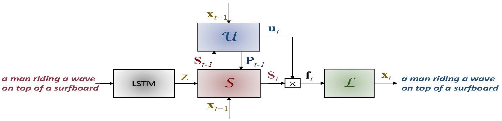
Figure 5: Pre-training of TPGN.

Fig. 5 shows a pre-training method for initializing TPGN. During the pre-training phase, there is no image input, i.e., image feature vector ${\mathbf{v}}=0$. In Fig. 5, at time $t=-T+1$, the LSTM module takes a sentence of length $T$ as input and outputs a vector ${\mathbf{z}}$ (${\mathbf{z}}\in\mathbb{R}^{d^{2}}$) at time $t=0$. That is, the LSTM converts a sentence into ${\mathbf{z}}$, which is the input of TPGN. We use end-to-end training to train the whole system shown in Fig. 5. After finishing pre-training, we let ${\mathbf{z}}=0$ and use images as input to train the TPGN in Fig. 3, initialized by the pretrained parameter values.

Appendix C Related work

Most existing DL-based image captioning methods [16, 11, 17, 18, 19, 6, 20, 21] involve two phases/modules: 1) image analysis, typically by a Convolutional Neural Network (CNN), and 2) a language model for caption generation ([22]). The CNN module takes an image as input and outputs an image feature vector or a list of detected words with their probabilities. The language model is used to create a sentence (caption) out of the detected words or the image feature vector produced by the CNN.

There are mainly two approaches to natural language generation in image captioning. The first approach takes the words detected by a CNN as input, and uses a probabilistic model, such as a maximum entropy (ME) language model, to arrange the detected words into a sentence. The second approach takes the penultimate activation layer of the CNN as input to a Recurrent Neural Network (RNN), which generates a sequence of words (the caption) [11].

The work reported here follows the latter approach, adopting a CNN + RNN-generator architecture. Specifically, instead of using a conventional RNN, we propose a recurrent network that has substructure derived from the general GSC architecture: one recurrent subnetwork holds an encoding $\mathbf{S}$ — which is treated as an approximation of a TPR — of the words yet to be produced, while another recurrent subnetwork generates a sequence of vectors that is treated as a sequence of roles to be unbound from $\mathbf{S}$, in effect, reading out a word at a time from $\mathbf{S}$. Examining how the model deploys these roles allows us to interpret them in terms of grammatical categories; roughly speaking, a sequence of categories is generated and the words stored in $\mathbf{S}$ are retrieved and spelled out via their categories.

References

- [1] “Wikipedia link for captcha,” https://en.wikipedia.org/wiki/CAPTCHA, 2017.
- [2] “Coco dataset for image captioning,” http://mscoco.org/dataset/#download, 2017.
- [3] P. Smolensky, “Tensor product variable binding and the representation of symbolic structures in connectionist systems,” Artificial intelligence, vol. 46, no. 1-2, pp. 159–216, 1990.
- [4] P. Smolensky and G. Legendre, The harmonic mind: From neural computation to optimality-theoretic grammar. Volume 1: Cognitive architecture. MIT Press, 2006.
- [5] P. Anderson, B. Fernando, M. Johnson, and S. Gould, “Spice: Semantic propositional image caption evaluation,” in European Conference on Computer Vision. Springer, 2016, pp. 382–398.
- [6] A. Karpathy and L. Fei-Fei, “Deep visual-semantic alignments for generating image descriptions,” in Proceedings of the IEEE Conference on Computer Vision and Pattern Recognition, 2015, pp. 3128–3137.
- [7] Z. Gan, C. Gan, X. He, Y. Pu, K. Tran, J. Gao, L. Carin, and L. Deng, “Semantic compositional networks for visual captioning,” in Proceedings of the IEEE Conference on Computer Vision and Pattern Recognition, 2017.
- [8] K. He, X. Zhang, S. Ren, and J. Sun, “Deep residual learning for image recognition,” in Proceedings of the IEEE Conference on Computer Vision and Pattern Recognition, 2016, pp. 770–778.
- [9] J. Pennington, R. Socher, and C. Manning, “Stanford glove: Global vectors for word representation,” https://nlp.stanford.edu/projects/glove/, 2017.
- [10] M. Abadi, A. Agarwal, P. Barham, E. Brevdo, Z. Chen, C. Citro, G. S. Corrado, A. Davis, J. Dean, M. Devin, S. Ghemawat, I. Goodfellow, A. Harp, G. Irving, M. Isard, Y. Jia, R. Jozefowicz, L. Kaiser, M. Kudlur, J. Levenberg, D. Mané, R. Monga, S. Moore, D. Murray, C. Olah, M. Schuster, J. Shlens, B. Steiner, I. Sutskever, K. Talwar, P. Tucker, V. Vanhoucke, V. Vasudevan, F. Viégas, O. Vinyals, P. Warden, M. Wattenberg, M. Wicke, Y. Yu, and X. Zheng, “TensorFlow: Large-scale machine learning on heterogeneous systems,” 2015, software available from tensorflow.org. [Online]. Available: https://www.tensorflow.org/
- [11] O. Vinyals, A. Toshev, S. Bengio, and D. Erhan, “Show and tell: A neural image caption generator,” in Proceedings of the IEEE Conference on Computer Vision and Pattern Recognition, 2015, pp. 3156–3164.
- [12] K. Papineni, S. Roukos, T. Ward, and W.-J. Zhu, “Bleu: a method for automatic evaluation of machine translation,” in Proceedings of the 40th annual meeting on association for computational linguistics. Association for Computational Linguistics, 2002, pp. 311–318.
- [13] S. Banerjee and A. Lavie, “Meteor: An automatic metric for mt evaluation with improved correlation with human judgments,” in Proceedings of the ACL workshop on intrinsic and extrinsic evaluation measures for machine translation and/or summarization. Association for Computational Linguistics, 2005, pp. 65–72.
- [14] R. Vedantam, C. Lawrence Zitnick, and D. Parikh, “Cider: Consensus-based image description evaluation,” in Proceedings of the IEEE Conference on Computer Vision and Pattern Recognition, 2015, pp. 4566–4575.
- [15] P. Smolensky, “Symbolic functions from neural computation,” Philosophical Transactions of the Royal Society — A: Mathematical, Physical and Engineering Sciences, vol. 370, pp. 3543 – 3569, 2012.
- [16] J. Mao, W. Xu, Y. Yang, J. Wang, Z. Huang, and A. Yuille, “Deep captioning with multimodal recurrent neural networks (m-rnn),” in Proceedings of International Conference on Learning Representations, 2015.
- [17] J. Devlin, H. Cheng, H. Fang, S. Gupta, L. Deng, X. He, G. Zweig, and M. Mitchell, “Language models for image captioning: The quirks and what works,” arXiv preprint arXiv:1505.01809, 2015.
- [18] X. Chen and C. Lawrence Zitnick, “Mind’s eye: A recurrent visual representation for image caption generation,” in Proceedings of the IEEE Conference on Computer Vision and Pattern Recognition, 2015, pp. 2422–2431.
- [19] J. Donahue, L. Anne Hendricks, S. Guadarrama, M. Rohrbach, S. Venugopalan, K. Saenko, and T. Darrell, “Long-term recurrent convolutional networks for visual recognition and description,” in Proceedings of the IEEE conference on computer vision and pattern recognition, 2015, pp. 2625–2634.
- [20] R. Kiros, R. Salakhutdinov, and R. Zemel, “Multimodal neural language models,” in Proceedings of the 31st International Conference on Machine Learning (ICML-14), 2014, pp. 595–603.
- [21] R. Kiros, R. Salakhutdinov, and R. S. Zemel, “Unifying visual-semantic embeddings with multimodal neural language models,” arXiv preprint arXiv:1411.2539, 2014.
- [22] H. Fang, S. Gupta, F. Iandola, R. K. Srivastava, L. Deng, P. Dollár, J. Gao, X. He, M. Mitchell, J. C. Platt et al., “From captions to visual concepts and back,” in Proceedings of the IEEE conference on Computer Vision and Pattern Recognition, 2015, pp. 1473–1482.