An asymptotic analysis of distributed nonparametric methods

Abstract

We investigate and compare the fundamental performance of several distributed learning methods that have been proposed recently. We do this in the context of a distributed version of the classical signal-in-Gaussian-white-noise model, which serves as a benchmark model for studying performance in this setting. The results show how the design and tuning of a distributed method can have great impact on convergence rates and validity of uncertainty quantification. Moreover, we highlight the difficulty of designing nonparametric distributed procedures that automatically adapt to smoothness.

1 Introduction

Both in statistics and machine learning there has been substantial interest in the design and study of distributed statistical or learning methods in recent years. One driving reason is the fact that in certain applications datasets have become so large that it is often unfeasible, or computationally undesirable, to carry out the analysis on a single machine. In a distributed method the data are divided over a cluster consisting of several machines and/or cores. The machines in the cluster then process their data locally, after which the local results are somehow aggregated on a central machine to finally produce the overall outcome of the statistical analysis. Distributed methods are not only used for computational reasons, but are for instance also of interest in situations where privacy is important and it is undesirable that all data are handled at a single location. Moreover, there are applications in which data are by construction gathered at multiple locations and first processed locally, before being combined at a central location.

Over the last years a variety of distributed methods have been proposed. Recent examples include Consensus Monte Carlo (Scott et al. (2016)), WASP (Srivastava et al. (2015)), and distributed GP’s (Deisenroth and Ng (2015)), to mention but a few. Most papers on distributed methods do extensive experiments on simulated, benchmark and real data to numerically assess and compare the performance of the various methods. Some papers also derive a number of theoretical properties. Theoretical results on the performance of distributed methods are not yet widely available however and there is certainly no common theoretical framework in place that allows a clear theoretical comparison of methods and the development of an understanding of fundamental performance guarantees and limitations.

Since a better theoretical understanding of distributed methods can help to pinpoint fundamental difficulties and opportunities, we develop a framework in this paper which allows us to study and compare the performance of various methods. We are in particular interested in high-dimensional, or nonparametric problems. It is by now well known that the performance of learning or statistical methods in such settings depends crucially on wether or not a method succeeds in realizing the correct bias-variance trade-off, or, in different terminology, succeeds in balancing under- and overfitting. For classical, non-distributed settings we have a rather well-developed understanding of how methods should be tuned to achieve a proper bias-variance trade-off. For distributed methods however, such theory is currently not yet available.

To be able to develop relevant theory we study an idealized model, which is a distributed version of the canonical “signal-in-white-noise” model that serves as an important benchmark model in mathematical statistics (see for instance Tsybakov (2009); Johnstone (2017); Giné and Nickl (2016)). The model is on the one hand rich enough to be interesting, in the sense that it is really distributed in nature and the unknown object that needs to be learned is truly infinite-dimensional. On the other hand it is tractable enough to allow detailed mathematical analysis. In the non-distributed case the signal-in-white-noise model is well known to be very closely related to other nonparametric models, such as nonparametric regression and density estimation. (This can be made very precise in the context of Le Cam’s theory of limits of experiments (e.g. Le Cam (2012), Brown and Low (1996), Nussbaum (1996)).) Similarly, the distributed signal-in-white-noise model that we consider in this paper provides a unified framework to compare methods that were originally introduced in different settings. We introduce the model in Section 2.

It is not difficult to see that if the number of machines $m$ is relatively large with respect to the total sample size, or signal-to-noise-ratio $n$, then doing things completely naively in the distributed case leads to a sub-optimal bias-variance trade-off (see also the simulation example in Section 2). In particular, just computing the “usual” estimators on every local machine and then averaging them on the central machine typically leads to a global estimator with a bias that is too large. To achieve good performance, the trade-off has to be adjusted somehow. This can in principle be done in various ways. For instance by locally choosing the “wrong” settings for tuning parameters on purpose, or, in a Bayesian setting, by adjusting the likelihood (e.g. raising it to some power) or by adjusting the prior. In Section 3 we study to what degree various methods that have been proposed in the literature succeed in ultimately achieving the right trade-off. We will see that some are more successful than others in this respect.

An important observation that we make is that the methods that are shown to work well in Section 3 all use information on aspects of the true signal that are in principle unknown, such as its degree of regularity. A key question is whether in distributed settings it is fundamentally possible to set tuning parameters correctly in a purely data-driven way, without using such information. In the non-distributed setting it is well known that such adaptive methods indeed exist (e.g. Tsybakov (2009) or Giné and Nickl (2016)). In the distributed case that we study here however, this is much less clear. In Section 4 we show that using a distributed version of a standard adaptation method that is known to work in the non-distributed case, such as maximum marginal likelihood empirical Bayes, can lead to sub-optimal results in the distributed setting. We will argue that this seems to be a fundamental issue and that we expect that correct automatic setting of tuning parameters in distributed methods is fundamentally more challenging than in the classical, non-distributed case. We believe this is an important issue and want to highlight it as an important and interesting topic for future research.

The remainder of the paper is organized as follows. In the next section we introduce the distributed version of the signal-in-white-noise model and provide a simple simulation example to show that in a distributed setting, naively combining inferences from local machines into a global estimator may produce misleading results. In Section 3 we study the performance of a number of Bayesian procedures for signal reconstruction in the distributed signal-in-white-noise model introduced in Section 2. We include a number of methods that have recently been proposed in the literature. We show that some succeed in obtaining the appropriate bias-variance trade-off, but others do not. Moreover, the ones that do produce good results are all non-adaptive, in the sense that they use knowledge of the smoothness of the unkown signal to set their tuning parameters. In the final Section 4 we consider the more realistic setting in which this smoothness is unknown. We study a distributed method that has been proposed for data-driven tuning of the hyperparameters and show that there exist “difficult signals”, which this method can not recover in the distributed model at an optimal rate. We argue that this appears to be a fundamental issue, and that designing procedures that automatically adapt to smoothness is fundamentally more challenging in the distributed framework. Mathematical proofs are collected in appendix Sections A and B.

2 Distributed signal-in-white-noise model

Consider the problem of estimating a signal $\theta\in\ell^{2}$ in Gaussian white noise. In the usual setting there is a single observer that observes every coefficient $\theta_{i}$ with additive Gaussian noise with variance $\sigma^{2}/n$, say. In the distributed version of the model we divide the “precision budget” $n$ over $m$ different observers, so that each one observes the signal in Gaussian noise with variance $\sigma^{2}m/n$, independent of the others. In other words, observer $j$ has data $Y^{j}_{1},Y^{j}_{2},\ldots$ satisfying

$$Y^{j}_{i}=\theta_{i}+\sqrt{\frac{\sigma^{2}m}{n}}Z^{j}_{i},\qquad i=1,2,\ldots,$$ (2.1)

where the $Z^{j}_{i}$ are independent, standard Gaussian random variables. We call the $m$ independent sub-problems in which the signal-to-noise ratio is $\sigma^{2}m/n$ the “local” problems.

The classical, non-distributed signal-in-white-noise model is obtained from the distributed model by aggregating all the local data. Indeed, if for $j=1,2,\ldots$ we define $Y_{i}=m^{-1}\sum_{j=1}^{m}Y^{j}_{i}$, then

$$Y_{i}=\theta_{i}+\sqrt{\frac{\sigma^{2}}{n}}\tilde{Z}_{i},\qquad i=1,2,\ldots,$$ (2.2)

where the $\tilde{Z}_{i}=m^{-1/2}\sum_{j=1}^{m}Z^{j}_{i}$ are independent standard normal variables. This model has been studied extensively in the literature, serving as a canonical model for understanding the performance of high-dimensional or nonparametric statistical procedures. It is well known for instance that if the true signal $\theta$ belongs to an ellipsoid or a hyper rectangle of the form

$$\{\theta\in\ell^{2}:\sum i^{2\beta}\theta_{i}^{2}\leq M^{2}\}\ \text{or}\ \{\theta\in\ell^{2}:\,\sup_{i}(i^{1+2\beta}\theta_{i}^{2})\leq M^{2}\}$$

for some $\beta,M>0$, then the optimal rate of convergence of estimators (relative to the $\ell^{2}$-norm) is of the order $n^{-\beta/(1+2\beta)}$. Moreover, there exist so-called adaptive estimators, which achieve this rate without using knowledge about the parameters $\beta$ or $M$ that describe the complexity, or regularity of the true signal. See, for instance, Tsybakov (2009) or Giné and Nickl (2016). Our central question is whether or not the same results can be obtained in the distributed setting in which each of the $m$ different observers first separately make inference about the signal, and then the local estimates are aggregated into one joint estimator.

The specific examples of distributed procedures that we consider in this paper are about distributed Bayesian methods. These methods have in common that each local observer first chooses a prior distribution and computes the corresponding local posterior distribution using the local data (or an appropriate modification). In the next step the $m$ local posteriors are somehow aggregated into a global posterior-type distribution, which is then used to produce an estimate of the signal and/or a quantification of the associated uncertainty. In general there is no guarantee that this “aggregated posterior” resembles the posterior distribution that would be obtained in the non-distributed setting, using all the data at once. In particular, it is not clear beforehand how a distributed Bayes method should be constructed in order to have good theoretical properties, like optimal convergence rates or adaptation properties. In this paper we investigate various distributed methods that have been proposed from this point of view.

To see that interesting things can happen it is exemplifying to compare the results of a distributed and a non-distributed (Bayesian) analysis of simulated data. Concretely, we consider a true signal $\theta$ consisting of the Fourier coefficients of the function shown in Figure 1.

Figure 1: True signal.

For this signal we simulate data according to (2.1), with $\sigma=1$, $m=40$ and $n=120\times 40=4800$. Then for every local observer a Bayesian procedure is carried out with a Gaussian prior on $\theta$, postulating that the coordinates $\theta_{i}$ are independent and $N(0,i^{-1-2\alpha})$-distributed. The hyperparameter $\alpha$, which describes the regularity of the prior, is determined using a distributed version of maximum marginal likelihood, as described in Section 4. This analysis leads to $m=40$ local posterior distributions. These are then combined to produce an overall posterior distribution for the signal. The precise procedure is described in Section 4. The resulting estimator for the signal, together with pointwise $95\%$ credible intervals, is shown in the left plot in Figure 2.

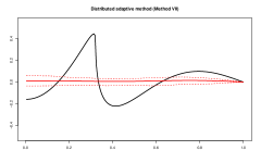
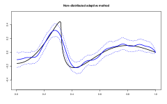
Figure 2: Signal reconstruction using the distributed method (left) and the non-distributed method (right).

The corresponding non-distributed result is obtained by first aggregating all local data as in (2.2) and then carrying out the same Bayesian procedure on these complete data. The resulting non-distributed reconstruction of the signal is shown on the right in Figure 2.

The non-distributed version of this method was studied theoretically for instance in Knapik et al. (2016) and Szabó et al. (2015), where it was shown that the method is adaptive and rate-optimal. The simulation suggests however that an apparently reasonable distributed analogue of the method does not necessarily inherit these favourable properties. The procedure seems to be underfitting and the credible intervals appear to be too narrow. We will argue that this is in some sense a fundamental issue and in the next sections we will study various proposed distributed methods to investigate to what degree they succeed in avoiding or solving these problems.

3 Results for non-adaptive procedures

In this section we study the performance of a number of Bayesian procedures for signal reconstruction in the distributed signal-in-white-noise model introduced in Section 2. All methods involve putting a prior distribution on the unknown signal $\theta\in\ell^{2}$ in each local problem and then combining the resulting local posteriors into one global posterior-type distribution. To be able to compare the various methods we consider the same Gaussian process (GP) prior in every case, namely the prior

$$\Pi(\cdot|\alpha)=\bigotimes_{i=1}^{\infty}N(0,i^{-1-2\alpha}),$$ (3.1)

which postulates that the coefficients $\theta_{i}$ of the signal $\theta$ are independent and $N(0,i^{-1-2\alpha})$-distributed. The hyper parameter $\alpha>0$ controls the regularity of the prior. (Some of the methods we consider use exactly this prior, others modify it in a certain way with the aim of achieving better performance.) The global posterior-type distribution depends on all the data $\mathbf{Y}=(Y^{j}_{i}:j=1,\ldots,m;i=1,2,\ldots)$ and is denoted by $\Pi(\cdot\,|\,\mathbf{Y})$. It is generally some type of average of the local posteriors, but its precise construction differs between proposed methods. We will see that this can have a significant effect on performance.

We take an asymptotic perspective and investigate in every case the rate at which the global posterior contracts around the true signal as $n\to\infty$ relative to the $\ell^{2}$-norm, which is as usual defined by $\|\theta\|^{2}_{2}=\sum\theta_{i}^{2}$. For a sequence of positive numbers $\varepsilon_{n}\to 0$ we say that the global posterior contracts at the rate $\varepsilon_{n}$ around the true signal $\theta_{0}$ if for all sequences $M_{n}\to\infty$,

$${\rm E}_{\theta_{0}}\Pi(\theta\in\ell^{2}:\|\theta-\theta_{0}\|_{2}>M_{n}\varepsilon_{n}\,|\,\mathbf{Y})\to 0$$

as $n\to\infty$. This means that asymptotically, all posterior mass is concentrated in balls around the true signal $\theta_{0}$ with $\ell^{2}$-radius of the order $\varepsilon_{n}$.

Additionally, we study how well the posterior quantifies the remaining uncertainty. Specifically, we consider the coverage probabilities of credible balls around the global posterior mean. These credible sets are constructed by first computing the mean $\hat{\theta}$ of the global “posterior” $\Pi(\cdot\,|\,\mathbf{Y})$. Then for a level $\gamma\in(0,1)$, the posterior is used to determine the radius $r_{\gamma}$ such that the ball around $\hat{\theta}$ with radius $r_{\gamma}$ receives $1-\gamma$ posterior mass, i.e.

$$\Pi(\theta:\,\|\theta-\hat{\theta}\|_{2}\leq r_{\gamma}|\mathbf{Y})=1-\gamma.$$

For $L>0$, the credible set $\hat{C}(L)$ is subsequently defined by

$$\hat{C}(L)=\{\theta:\,\|\theta-\hat{\theta}_{n}\|_{2}\leq Lr_{\gamma}\}.$$ (3.2)

(The extra constant $L$ gives some added flexibility, for $L=1$ we obtain an exact $1-\gamma$ credible set.) We are interested in the coverage probabilities ${\rm P}_{\theta_{0}}(\theta_{0}\in\hat{C}(L))$. If this tends to $0$ as $n\to\infty$, the credible sets are asymptotically not frequentist confidence sets, hence give a misleading quantification of the uncertainty. Ideally, the coverage probabilities stay bounded away from $0$ as $n\to\infty$.

In the non-distributed case $m=1$ it is well known that both the rate at which the posterior contracts around the truth and the behaviour of the coverage probabilities of credible sets depend crucially on how the hyper parameter $\alpha$ is tuned. The correct bias-variance trade-off is achieved if $\alpha$ is in accordance with the regularity of the unknown signal. To make this precise, we will consider signals belonging to hyper rectangles of the form

$$H^{\beta}(M)=\Big{\{}\theta\in\ell^{2}:\sup_{i}(i^{1+2\beta}\theta^{2}_{i})\leq M^{2}\Big{\}}$$ (3.3)

for some $\beta,M>0$. It is shown for instance in Knapik et al. (2011) for the non-distributed case that if $\theta_{0}\in H^{\beta}(M)$ and we set $\alpha=\beta$, then the posterior contracts around $\theta_{0}$ at the optimal rate $n^{-\beta/(1+2\beta)}$. Moreover, for $L$ large enough it then holds that ${\rm P}_{\theta_{0}}(\theta_{0}\not\in\hat{C}(L))\leq\gamma$. Hence, in the non-distributed case it is optimal to choose the hyper parameter $\alpha$ in such a way that the regularity $\alpha$ of the prior matches the regularity $\beta$ of the true signal. Moreover, this choice leads to a contraction rate that is optimal in a minimax sense.

In the remainder of this section we investigate distributed methods from this point of view. We will see that the different proposed methods lead to different behaviours in terms of contraction rates and coverage. We stress that the results in this section are non-adaptive, in the sense that we allow the tuning parameter $\alpha$ and other aspects of the constructions to use knowledge of the regularity $\beta$ of the true signal. This is of course not realistic. It is however important to first understand for every method whether ideally, if the value of $\beta$ is given to us by an oracle, it is possible to tune the method optimally. Whether this is also possible adaptively, without knowing $\beta$, is then the next natural question, which we address in Section 4.

3.1 Naive averaging of local posterior draws

Recall that we have $m$ local observers that each have a dataset $\mathbf{Y}^{j}=(Y^{j}_{1},Y^{j}_{2},\ldots)$ of noisy coefficients satisfying (2.1). The aim is to recover the true sequence of coefficients $\theta$.

As a starting point, and to have a baseline case to compare the other methods to, we analyse the naive distributed approach in which in every local problem we simply use the prior $\Pi(\cdot\,|\,\alpha)$ defined by (3.1), with $\alpha=\beta$ equal to the regularity of the true sequence $\theta$, in the sense of (3.3). Every local observer then computes its corresponding local posterior, $\Pi^{j}(\cdot\,|\,\mathbf{Y}^{j})$. By Bayes’ formula this is given by

$$d\Pi^{j}(\theta\,|\,\mathbf{Y}^{j})\propto p(\mathbf{Y}^{j}\,|\,\theta)\,d\Pi(\theta\,|\,\beta),$$

where the likelihood for the $j$th local problem is given by

$$p(\mathbf{Y}^{j}\,|\,\theta)\propto\prod e^{-\frac{1}{2}\frac{n(Y^{j}_{i}-\theta_{i})^{2}}{\sigma^{2}m}}.$$ (3.4)

Finally these local posteriors are combined into a global, “average posterior” ${\mathbf{\Pi}_{I}(\cdot\,|\,\mathbf{Y})}$ by postulating that a draw from this global posterior is generated by first drawing once from each local posterior and then averaging these $m$ independent draws. (Formally, this means that the global “posterior” ${\mathbf{\Pi}_{I}(\cdot\,|\,\mathbf{Y})}$ is the convolution of the rescaled local posteriors $\Pi^{1}(m\times\cdot\,|\,\mathbf{Y}^{1})$, …, $\Pi^{m}(m\times\cdot\,|\,\mathbf{Y}^{m})$).

This distributed method is conceptually very simple, but it turns out that neither from the point of view of contraction rates, nor from the point of view of uncertainty quantification it performs very well. The reason is basically that although the choice $\alpha=\beta$ of the tuning parameter of the prior correctly matches squared bias, variance and posterior spread in the local problems, the averaging procedure results in a global “posterior” for which the spread and the variance of the mean are too small relative to the squared bias. The following theorem asserts that for every smoothness level $\beta>0$ there exist $\beta$-regular truths for which the contraction rate of the posterior deteriorates substantially and for which the uncertainty quantification by the credible sets (3.2) constructed from the global posterior ${\mathbf{\Pi}_{I}(\cdot\,|\,\mathbf{Y})}$ is useless, no matter how far they are blown up by a constant $L>0$.

Theorem 3.1 (naive averaging).

For every $\beta,M>0$ there exists a $\theta_{0}\in H^{\beta}(M)$ such that for small enough $c>0$,

$$E_{\theta_{0}}\mathbf{\Pi}_{I}(\theta:\,\|\theta-\theta_{0}\|_{2}\leq cm^{\frac{\beta}{1+2\beta}}n^{-\frac{\beta}{1+2\beta}}|\beta,\mathbf{Y})\rightarrow 0$$

as $m\to\infty$ and $n/m\to\infty$. Furthermore, for all $L>0$ it holds that

$$P_{\theta_{0}}\big{(}\theta_{0}\in\hat{C}(L)\big{)}\rightarrow 0.$$

Proof.

The proof of the theorem is given in Section A.1. ∎

In the literature several less naive distributed strategies have been proposed. These methods either change the local likelihoods in a certain way, and/or the priors that are locally used, and/or the way that the local posteriors are aggregated. In the next few sections we investigate whether such strategies can improve the bad asymptotic performance of the naive averaging method.

3.2 Adjusted local likelihoods and averaging

One perspective on the bad performance of the naive method is to say that since the “sample size” $n/m$ in the local problems is too small, the influence of the data on the local posterior is too small, resulting in a variance (and spread) that is too small relative to the squared bias. A possible way to remedy this that has been proposed in several papers is to raise the local likelihoods to the power $m$, in order to mimic the situation that we have sample size $n$ in the local problems. This generalized Bayesian approach for the local problems has for instance been considered in the distributed context by Srivastava et al. (2015). They combine it with a different aggregation method however, which we consider in Section 3.4. In this section we still consider the simple averaging scheme, in order to isolate the effect of adjusting the local likelihoods.

So in method II all local observers use the prior $\Pi(\cdot\,|\,\alpha)$ again, with $\alpha=\beta$ equal to the regularity of the truth. They now each compute a generalized local posterior $\tilde{\Pi}^{j}(\cdot\,|\,\mathbf{Y}^{j})$, defined by

$$d\tilde{\Pi}^{j}(\theta\,|\,\mathbf{Y}^{j})\propto\Big{(}p(\mathbf{Y}^{j}\,|\,\theta)\Big{)}^{m}\,d\Pi(\theta\,|\,\beta).$$

As before the global “posterior” ${\mathbf{\Pi}_{II}(\cdot\,|\,\mathbf{Y})}$ is defined by postulating that a draw from this global posterior is generated by first drawing once from each local generalized posterior and then averaging these $m$ independent draws.

The following theorem states that this method indeed improves the naive approach of Section 3.1. The global posterior now contracts at the optimal rate for every $\beta$-regular truth. Unfortunately, the bad behaviour of the credible sets has not been remedied. For this approach the uncertainty quantification is in fact misleading for all $\beta$-regular truths.

Theorem 3.2 (adjusted likelihoods + averaging).

For all $\beta,M>0$ and all sequences $M_{n}\to\infty$,

$$\sup_{\theta_{0}\in H^{\beta}(M)}{\rm E}_{\theta_{0}}\mathbf{\Pi}_{{II}}(\theta:\,\|\theta-\theta_{0}\|_{2}\geq M_{n}n^{-\frac{\beta}{1+2\beta}}|\mathbf{Y})\rightarrow 0$$

as $n,m\to\infty$. However, for all $\theta_{0}\in H^{\beta}(M)$ and all $L>0$ it holds that

$${\rm P}_{\theta_{0}}\big{(}\theta_{0}\in\hat{C}(L)\big{)}\rightarrow 0.$$

Proof.

The proof is given in Section A.2. ∎

3.3 Adjusted priors and averaging

Adjusting the likelihood as in the preceding section resulted in a correct trade-off between the bias and the variance of the global posterior mean, yielding an optimal posterior contraction rate. The spread of the posterior remained too small in comparison however, resulting in credible sets with zero asymptotic coverage. Instead of raising the local posteriors to the power $m$, as considered in the preceding section, we could alternatively raise the prior density to the power $1/m$. This has for instance been proposed in the context of the “Consensus Monte Carlo” approach by Scott et al. (2016), in combination with simple averaging of the local posteriors. In this section we investigate the performance of this method in terms of posterior contraction and uncertainty quantification in our distributed signal-in-white-noise model.

The prior $\Pi(\cdot\,|\,\alpha)$ that we use in the local problems is again a product of centered Gaussians with variance $i^{-1-2\alpha}$. Raising the corresponding densities to the power $1/m$ has the effect of multiplying the $i$th prior variance by $m$. Hence, in our case raising the prior density to the power $1/m$ is the same as multiplicative rescaling, postulating that $\theta$ is a-priori distributed according to $\Pi(\cdot\,|\,\alpha,m)$, where

$$\Pi(\cdot|\alpha,\tau)=\bigotimes_{i=1}^{\infty}N(0,\tau i^{-1-2\alpha})$$ (3.5)

for $\alpha,\tau>0$. Rescaled GPs have also been considered by Shang and Cheng (2015), who have used them in the distributed setting to construct global credible sets from local ones.

Using rescaling we can actually obtain good results if the prior regularity $\alpha$ is not exactly equal to the true regularity $\beta$. By using a scaling different from $\tau=m$ we can somehow compensate for the mismatch between $\alpha$ and $\beta$, at least in the range $\beta\leq 1+2\alpha$. In the non-distributed setting this is a well-known phenomenon, see for instance van der Vaart and van Zanten (2007); Knapik et al. (2011); Szabó et al. (2013).

The distributed procedure that we consider in this section then takes the following form. Every local observer uses the rescaled prior $\Pi(\cdot|\alpha,\tau)$ defined by (3.5), with $\alpha>0$ and

$$\tau=mn^{\frac{2(\alpha-\beta)}{1+2\beta}},$$

where $\beta$ is the regularity of the truth. Next the (normal, unadjusted) corresponding posteriors are computed and they are averaged into a global “posterior” $\mathbf{\Pi}_{III}(\cdot\,|\,\mathbf{Y})$ as in the preceding sections. (Note that if in the local problems the prior regularity $\alpha=\beta$ is used, then $\tau=m$, so the method corresponds to raising the prior density to the power $1/m$.)

The following theorem gives the posterior contraction and coverage results for this method.

Theorem 3.3 (adjusted priors + averaging).

Suppose $\beta,M>0$ and $\beta\leq 1+2\alpha$. Then for all sequences $M_{n}\to\infty$,

$$\sup_{\theta_{0}\in H^{\beta}(M)}{\rm E}_{\theta_{0}}\mathbf{\Pi}_{III}(\theta:\,\|\theta-\theta_{0}\|_{2}>M_{n}n^{-\frac{\beta}{1+2\beta}}|\mathbf{Y})\rightarrow 0$$

as $n\to\infty$. Moreover, for all $\gamma\in(0,1)$ it holds that

$$\sup_{\theta_{0}\in H^{\beta}(M)}{\rm P}_{\theta_{0}}\Big{(}\theta_{0}\not\in\hat{C}(L)\Big{)}\leq\gamma$$

for large enough $L>0$.

Proof.

See Section A.3. ∎

So adjusting the prior in this way actually works better than adjusting the likelihood. Not only do we get optimal contraction rates, but the credible sets that this method produces have asymptotic coverage too. The proof shows that the credible sets have optimal radius of the order $n^{-\beta/(1+2\beta)}$ as well.

3.4 Adjusted local likelihoods and Wasserstein barycenters

In Section 3.2 we saw that raising the local likelihoods to the power $m$ and then averaging the corresponding generalized posteriors yields optimal contraction rates, but can produce badly performing credible sets. In this section we study the approach considered by Minsker et al. (2014); Srivastava et al. (2015) in the context of their “WASP” method, which consists in aggregating the local posteriors not by simple averaging, but by computing their Wasserstein barycenter.

The generalized local posteriors $\tilde{\Pi}^{j}(\cdot\,|\,\mathbf{Y}^{j})$, as defined in Section 3.2, are (Gaussian) measures on $\ell^{2}$. The $2$-Wasserstein distance $W_{2}(\mu,\nu)$ between two probability measures $\mu$ and $\nu$ on $\ell^{2}$ is defined by

$$W^{2}_{2}(\mu,\nu)=\inf_{\gamma}\int\!\!\int\|x-y\|_{2}^{2}\,\gamma(dx,dy),$$

where the infimum is over all measures $\gamma$ on $\ell^{2}\times\ell^{2}$ with marginals $\mu$ and $\nu$. The corresponding 2-Wasserstein barycenter of $m$ probability measures $\mu_{1},\ldots,\mu_{m}$ on $\ell^{2}$ is then defined by

$$\bar{\mu}=\mathop{\rm argmin}_{\mu}\frac{1}{m}\sum_{j=1}^{m}W^{2}_{2}(\mu,\mu_{j}),$$

where the minimum is over all probability measures on $\ell^{2}$ with finite second moments. There exist effective algorithms to compute Wasserstein barycenters in many cases, see for instance Cuturi and Doucet (2014) and the references therein.

Having this notion at our disposal the distributed method we consider in this section proceeds as follows. In every local problem the prior $\Pi(\cdot\,|\,\alpha)$ is used, with $\alpha=\beta$ equal to the regularity of the truth. Next, the corresponding generalized posteriors $\tilde{\Pi}^{j}(\cdot\,|\,\mathbf{Y}^{j})$ are computed locally, which involves raising the likelihood to the power $m$ as described in Section 3.2. Finally, the global “posterior” $\mathbf{\Pi}_{IV}(\cdot\,|\,\mathbf{Y})$ is constructed as the 2-Wasserstein barycenter of the local measures $\tilde{\Pi}^{1}(\cdot\,|\,\mathbf{Y}^{1}),\ldots,\tilde{\Pi}^{m}(\cdot\,|\,\mathbf{Y}^{m})$.

The following theorem asserts that this method results in optimal posterior contraction rates and correct quantification of uncertainty.

Theorem 3.4 (adjusted likelihoods + barycenters).

For all $\beta,M>0$ and all sequences $M_{n}\to\infty$,

$$\sup_{\theta_{0}\in H^{\beta}(M)}{\rm E}_{\theta_{0}}\mathbf{\Pi}_{IV}(\theta:\,\|\theta-\theta_{0}\|_{2}>M_{n}n^{-\frac{\beta}{1+2\beta}}|\mathbf{Y})\rightarrow 0$$

as $n\to\infty$. Moreover, for all $\gamma\in(0,1)$ it holds that

$$\sup_{\theta_{0}\in H^{\beta}(M)}{\rm P}_{\theta_{0}}\Big{(}\theta_{0}\not\in\hat{C}(L)\Big{)}\leq\gamma$$

for large enough $L>0$.

Proof.

See Section A.4. ∎

3.5 Product of Gaussian process experts

The proofs of the theorems presented so far show that since in our context the global “posterior” is always a Gaussian measure, the behaviour of the procedure can be understood by analyzing three central quantities: the bias of the posterior mean, the variance of the posterior mean, and the spread of the posterior. Depending on how these quantities are related we have found different behaviours: sub-optimal posterior contraction and bad coverage of credible sets (Section 3.1), optimal posterior contraction but bad coverage of credible sets (Section 3.2), and optimal posterior contraction and also good coverage of credible sets (Sections 3.3 and 3.4).

In principle it is now straightforward to analyze different methods as well, provided the three central quantities can be controlled. As an illustration we consider in this section the single-layer version of the product-of-Gaussian-process-expert (PoE) model, introduced in Ng and Deisenroth (2014) and a generalization proposed in Cao and Fleet (2014). An interesting fact is that we will encounter a combination of behaviours that we have not seen yet: sub-optimal contraction rates, but good coverage of credible sets. These methods were introduced to deal with the distributed non-parametric regression model, but for the sake of comparison we analyze them in the context of our distributed signal-in-white-noise model, which can be thought of as an idealized version of the regression model.

The idea of the basic version of the Gaussian PoE model is to employ a Gaussian prior in every local machine, compute the corresponding posterior densities and approximate the global posterior density by multiplying and normalizing these. In our infinite-dimensional setting this does not make sense strictly speaking, since we can not express priors and posteriors on $\ell^{2}$ in terms of densities with respect to some generic dominating measure. We could remedy this by considering a truncated version of our distributed model, where we assume we only observe the first $n$ noisy coefficients $Y^{j}_{i}$ in every machine, say, and focus on making inference about the first $n$ true coefficients $\theta_{i}$. This would make the setting finite-dimensional, allowing us to write prior and posterior densities with respect to Lebesgue measure. Alternatively, we can stay in the infinite-dimensional setting of the paper and just reason formally and still arrive at a well-defined global PoE “posterior”. This is the approach we follow here.

Indeed, say that as before we use the prior $\Pi(\cdot\,|\,\alpha)$ given by (3.1) in every local machine, with $\alpha=\beta$ equal to the regularity of the true signal. This prior has formal “density” proportional to

$$\theta\mapsto\prod e^{-\tfrac{1}{2}\frac{\theta_{i}^{2}}{i^{-1-2\beta}}}.$$

By completing the square we see that the product of this expression with the local likelihood given by (3.4) is, still formally, proportional to

$$\theta\mapsto\prod e^{-\tfrac{1}{2}\frac{\theta_{i}^{2}}{i^{-1-2\beta}}}e^{-\frac{1}{2}\frac{n(Y^{j}_{i}-\theta_{i})^{2}}{\sigma^{2}m}}\propto\prod e^{-\frac{1}{2}\theta_{i}^{2}(i^{1+2\beta}+\frac{n}{m\sigma^{2}})+\theta_{i}\frac{nY^{j}_{i}}{m\sigma^{2}}}.$$

Taking the product over $j$ we then obtain the formal density of the PoE posterior, which is proportional to

$$\theta\mapsto\prod e^{-\frac{1}{2}\theta_{i}^{2}(mi^{1+2\beta}+\frac{n}{\sigma^{2}})+\theta_{i}\frac{n\sum_{j=1}^{m}Y^{j}_{i}}{m\sigma^{2}}}.$$

Now this last expression is, up to a constant, the density of a product of Gaussians with means $\hat{\theta}_{i}$ and variances $t^{2}_{i}$ given by

$$\hat{\theta}_{i}=\frac{nm^{-1}\sum Y^{j}_{i}}{n+\sigma^{2}mi^{1+2\beta}},\qquad t^{2}_{i}=\frac{\sigma^{2}}{n+\sigma^{2}mi^{1+2\beta}}.$$

The latter is in fact a well-defined Gaussian measure on $\ell^{2}$, so we can now simply define the global PoE “posterior” $\mathbf{\Pi}_{V}(\cdot\,|\,\mathbf{Y})$ as the latter measure.

We see that the expressions for the global mean and spread are in fact the same as what we found in Section A.1 for the naive averaging method. As a consequence, the negative result of Theorem 3.1 holds for the basic version of the Gaussian PoE model as well.

Theorem 3.5 (product of Gaussian experts).

For every $\beta,M>0$ there exists a $\theta_{0}\in H^{\beta}(M)$ such that for small enough $c>0$,

$${\rm E}_{\theta_{0}}\mathbf{\Pi}_{V}(\theta:\,\|\theta-\theta_{0}\|_{2}\leq cm^{\frac{\beta}{1+2\beta}}n^{-\frac{\beta}{1+2\beta}}|\mathbf{Y})\rightarrow 0$$

as $m\to\infty$ and $n/m\to\infty$. Furthermore, for all $L>0$ it holds that

$${\rm P}_{\theta_{0}}\big{(}\theta_{0}\in\hat{C}(L)\big{)}\rightarrow 0.$$

One can generalize the PoE model by raising the local posterior densities to some power before multiplying and normalizing them, as proposed in Cao and Fleet (2014). In the subsequent analysis we consider the choice to $1/m$ for the power, as suggested in Deisenroth and Ng (2015). Adapting the preceding analysis for the ordinary PoE model we see that for this generalized PoE model the global “posterior” $\mathbf{\Pi}_{VI}(\cdot\,|\,\mathbf{Y})$ is in our setting again a product of Gaussian, but now with means and variances given by

$$\hat{\theta}_{i}=\frac{nm^{-1}\sum Y^{j}_{i}}{n+\sigma^{2}mi^{1+2\beta}},\qquad t^{2}_{i}=\frac{\sigma^{2}m}{n+\sigma^{2}mi^{1+2\beta}}.$$

So the global posterior mean is unaltered compared to the basic PoE model, but the global posterior spread has been blown up by a factor $m$. As a result, there still exists the same class of truths as in Section A.1 for which the squared bias and the variance of the posterior mean will be incorrectly balanced, resulting in a sub-optimal rate of posterior contraction. However, the larger posterior spread ensures that we do have asymptotic coverage of credible sets. It should be noted however that these sets have a diameter that is sub-optimal, i.e. they are too conservative.

Theorem 3.6 (generalized product of Gaussian experts).

For every $\beta,M>0$ there exists a $\theta_{0}\in H^{\beta}(M)$ such that for small enough $c>0$,

$${\rm E}_{\theta_{0}}\mathbf{\Pi}_{VI}(\theta:\,\|\theta-\theta_{0}\|_{2}\leq cm^{\frac{\beta}{1+2\beta}}n^{-\frac{\beta}{1+2\beta}}|\mathbf{Y})\rightarrow 0$$

as $m\to\infty$ and $n/m\to\infty$. However, for all $\gamma\in(0,1)$ it holds that

$$\sup_{\theta_{0}\in H^{\beta}(M)}{\rm P}_{\theta_{0}}\Big{(}\theta_{0}\not\in\hat{C}(L)\Big{)}\leq\gamma$$

for large enough $L>0$.

Proof.

The proof of the theorem can be found in Section A.5. ∎

3.6 Summary of results for non-adaptive methods

We have seen that the various methods for aggregation of the local posteriors can give quite different results. The methods we considered produce different global “posterior” measures. Depending on the relation between the bias and variance of the global posterior mean and the spread of this global posterior, the posterior contraction rate and coverage probabilities of credible sets can have different behaviours. We summarize our findings in Table 1. This is certainly not meant to be an exhaustive list of methods, but rather an illustration of how the design of distributed procedures can affect their fundamental performance.

Method	Description	Optimal rate	Coverage
I	naive averaging	no	no
II	adjusted likelihoods, averaging	yes	no
III	adjusted priors, averaging	yes	yes
IV	adjusted likelihoods, barycenter	yes	yes
V	product of experts	no	no
VI	generalized product of experts	no	yes

Table 1: Performance of the various non-adaptive methods.

Simulations further illustrate the theoretical results. We have considered a true signal $\theta$ consisting of the Fourier coefficients of the function shown in the left panel of Figure 3. This is a signal which has regularity $\beta=1$ in the sense of (3.3). For this signal we simulated data according to (2.1), with $\sigma=1$, $n=4800$ and $m=40$, i.e. we considered a distributed setting with $m=40$ machines. For the sake of comparison, the right panel of Figure 3 shows the signal reconstruction and uncertainty quantification for the non-distributed method which first aggregates all data in a single machine and then computes the posterior corresponding to the prior $\Pi(\cdot\,|\,\alpha)$ defined by (3.1), with $\alpha=\beta$. This is a method which is known to have an optimal convergence rate and correct quantification of uncertainty. This classical, non-distributed result should be compared to Figure 4, which visualizes the “posteriors” generated by each of the distributed methods I–VI.

In accordance with our theoretical results, we see that the results of methods III and IV are comparable with the non-distributed method. Methods I, V and VI have worse signal reconstruction. The posterior mean of Method II is comparable to that of the optimal methods, but the uncertainty is underestimated.

Figure 3: Left: true signal. Right: posterior mean (blue solid curve) and $95\%$ pointwise credible bands (dashed blue curves) for the non-distributed method.

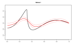
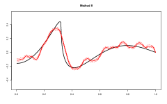
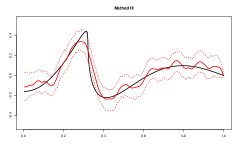
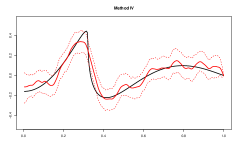
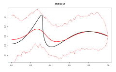
Figure 4: Global posterior mean (solid red curve) and $95\%$ pointwise credible bands (dashed red curves) for each of the methods I–VI.

An important observation to make is that the methods that achieve the same optimal performance as non-distributed methods, all use information about the regularity $\beta$ of the unkown signal, mostly through the setting of tuning parameters in the priors. In that sense, they are non-adaptive. They serve as useful results that indicate what is possible in principle if we have certain oracle knowledge about the truth we are trying to learn. To understand what realistic procedures can achieve this has to be combined with insight into what can be learned about this oracle knowledge from the data. In the next section we address this issue in the context of our distributed signal-in-white-noise model.

4 Results for adaptive procedures

In the non-distributed case it is well known that there exist adaptive methods that achieve the same optimal performance as non-adaptive procedures, without using knowledge of the regularity $\beta$ of the unkown signal. These methods somehow succeed in correctly trading off bias, variance (and spread in Bayesian methods) in a purely data-driven manner. For several such result in the context of the signal-in-white-noise model, see, for instance, Giné and Nickl (2016) and the references therein. For distributed methods the issue of adaptation appears to be a lot more subtle. In this paper we only have a first, negative result on adaptive properties of distributed methods.

So now we do not assume that we know the true regularity $\beta$ of the unknown signal. As before we employ the prior $\Pi(\cdot\,|\,\alpha)$ in the local machines. To tune the regularity parameter $\alpha$ of the prior we consider a distributed version of maximum marginal likelihood, as proposed by Deisenroth and Ng (2015). The usual, non-distributed version of that method would use the maximizer of the map

$$\alpha\mapsto\log\int\Big{(}\prod_{j=1}^{m}p(\mathbf{Y}^{j}\,|\,\theta)\Big{)}\,\Pi(d\theta\,|\,\alpha)$$

as tuning parameter. Maximizing this function however requires having all data available in a central machine. In the distributed setting, Deisenroth and Ng (2015) argue that this map is well approximated by the map

$$\alpha\mapsto\sum_{j=1}^{m}\log\Big{(}\int p(\mathbf{Y}^{j}\,|\,\theta)\,\Pi(d\theta\,|\,\alpha)\Big{)}.$$

Now every term in the sum just depends on one of the local machines and this function can be maximized on the central machine by repeatedly asking the local machines for function evaluations and gradients of the local log-marginal likelihoods

$$\log\int p(\mathbf{Y}^{j}\,|\,\theta)\,\Pi(d\theta\,|\,\alpha).$$

The resulting estimator is denoted by $\hat{\alpha}$, i.e.

$$\hat{\alpha}=\mathop{\rm argmax}_{\alpha\in[0,\log n]}\sum_{j=1}^{m}\log\Big{(}\int p(\mathbf{Y}^{j}\,|\,\theta)\,\Pi(d\theta\,|\,\alpha)\Big{)}.$$

(We maximize over a compact interval to ensure that the maximizer exists.)

It turns out that in the distributed setting, the local machines are in general not able to learn enough about the true signal regularity $\beta$. The following lemma asserts that there exist “difficult” signals for which the estimator $\hat{\alpha}$ overestimates the regularity.

Lemma 4.1.

For $\beta,M>0$, consider a signal $\theta_{0}\in\ell^{2}$ such that

$$\theta_{0,i}^{2}=\begin{cases}M^{2}i^{-1-2\beta}&\text{if $i\geq(n/(\sigma^{2}\sqrt{m}))^{1/(1+2\beta)}$},\\ 0&\text{else}.\end{cases}$$ (4.1)

Then $\theta_{0}\in H^{\beta}(M)$ and if $M$ is small enough, then

$${\rm P}_{\theta_{0}}(\hat{\alpha}\geq\beta+1/2)\to 1$$ (4.2)

if $n/m\to\infty$ and $m\to\infty$.

Proof.

The proof is given in Section B.1. ∎

In view of Lemma 4.1 it is perhaps not surprising that if the approximated maximum marginal likelihood estimator $\hat{\alpha}$ is used to tune the local prior that is used in every machine, sub-optimal performance is obtained for certain truths. Intuitively this is because due to the smaller signal-to-noise ratio, or “sample size” in the local machines, certain truths may appear more regular than they really are. It turns out that using the estimator $\hat{\alpha}$ in combination with any of the methods considered in the preceding section indeed leads to sub-optimal rates and bad coverage probabilities for certain truths. As an illustration we present a rigorous statement for the method of Section 3.4, but similar results can be derived for the others methods as well.

So suppose that in every local problem the prior $\Pi(\cdot\,|\,\alpha)$ is used, the corresponding generalized posterior $\tilde{\Pi}^{j}(\cdot\,|\,\mathbf{Y}^{j})$ is computed locally (which involves raising the local likelihood to the power $m$), and then the tuning parameter $\alpha$ is substituted by the estimator $\hat{\alpha}$ defined above. In the central machine, the global “posterior” $\mathbf{\Pi}_{VII}(\cdot\,|\,\mathbf{Y})$ is constructed as the 2-Wasserstein barycenter of the local “posterior” measures $\tilde{\Pi}^{1}(\cdot\,|\,\hat{\alpha},\mathbf{Y}^{1}),\ldots,\tilde{\Pi}^{m}(\cdot\,|\,\hat{\alpha},\mathbf{Y}^{m})$.

Theorem 4.2.

For $\beta,M>0$ and $\theta_{0}$ as in Lemma 4.1 we have, for some $c>0$,

$${\rm E}_{\theta_{0}}\mathbf{\Pi}_{VII}(\theta:\,\|\theta-\theta_{0}\|_{2}\leq c(n/\sqrt{m})^{-\frac{\beta}{1+2\beta}}|\mathbf{Y})\rightarrow 0$$

as $m\to\infty$ and $n/m\to\infty$. Furthermore, for all $L>0$ it holds that

$${\rm P}_{\theta_{0}}\big{(}\theta_{0}\in\hat{C}(L)\big{)}\rightarrow 0.$$

Proof.

See Section B.2. ∎

A simulation illustrating the theoretical result of theorem is given in Figure 2. The left panel visualizes the “posterior” generated by method VII, in the same distributed setting, and using the same simulated data as considered in Section 3.6.

So when combined with a data-driven tuning method like the distributed version of maximum marginal likelihood considered here, even the distributed methods that perform well in the non-adaptive setting loose their favourable properties. None of the methods yields a procedure that automatically adapts to regularity and achieves the optimal non-distributed rate. This does not imply of course that such an adaptive method does not exist. We expect however that the matter is delicate and that fundamental limitations exist.

The issue appears to be similar to that of the existence of adaptive confidence sets. To achieve adaptation in our distributed setting the local machines must be able to learn the “global” regularity of the signal from the limited local data that they have available. Analogous to the adaptive confidence problem we expect that this is in general only possible under additional assumptions on the true signal, like the self-similarity or polished tail conditions proposed for instance in Giné and Nickl (2010), Bull (2012), Szabó et al. (2015) , Nickl and Szabó (2016), Belitser et al. (2017). Making these admittedly somewhat loose claims mathematically precise will take considerably more effort, but seems an important and interesting direction for future work.

Appendix A Proofs for Section 3

A.1 Proof of Theorem 3.1

By completing the square we see that under the local posterior $\Pi^{j}(\cdot\,|\,\mathbf{Y}^{j})$ the coefficients $\theta_{i}$ are independent and Gaussian, with mean $\hat{\theta}^{j}_{i}$ and variance $s^{2}_{i}$ given by

$$\hat{\theta}^{j}_{i}=\frac{n}{n+\sigma^{2}mi^{1+2\beta}}Y^{j}_{i},\qquad s^{2}_{i}=\frac{\sigma^{2}m}{n+\sigma^{2}mi^{1+2\beta}}.$$

Hence the global “posterior” $\mathbf{\Pi}_{I}(\cdot\,|\,\mathbf{Y})$ is Gaussian as well, and under that measure the coefficients $\theta_{i}$ are independent and have mean $\hat{\theta}_{i}$ and variance $t^{2}_{i}$ given by

$$\hat{\theta}_{i}=\frac{1}{m}\sum_{j=1}^{m}\hat{\theta}^{j}_{i},\qquad t^{2}_{i}=\frac{s^{2}_{i}}{m}.$$

For the global posterior mean we have, for every $\theta_{0}\in\ell^{2}$,

$${\rm E}_{\theta_{0}}\,\hat{\theta}_{i}-\theta_{0,i}=\frac{-\sigma^{2}mi^{1+2\beta}}{n+\sigma^{2}mi^{1+2\beta}}\theta_{0,i},\qquad\mathrm{Var}_{\theta_{0}}\,\hat{\theta}_{i}=\frac{\sigma^{2}n}{(n+\sigma^{2}mi^{1+2\beta})^{2}},$$

and hence,

$${\rm E}_{\theta_{0}}\|\hat{\theta}-\theta_{0}\|^{2}_{2}=\sum\frac{\sigma^{4}m^{2}i^{2+4\beta}}{(n+\sigma^{2}mi^{1+2\beta})^{2}}\theta_{0,i}^{2}+\sum\frac{\sigma^{2}n}{(n+\sigma^{2}mi^{1+2\beta})^{2}}.$$

By Lemma A.1 of Szabó et al. (2013) the second, variance term is of the order

$$m^{-1/(1+2\beta))}n^{-2\beta/(1+2\beta)},$$

as $n/m\to\infty$. For $\theta^{2}_{0,i}=Mi^{-1-2\beta}$, by the same lemma, the first, squared bias term is proportional to $(n/m)^{-2\beta/(1+2\beta)}$. For the global spread, we have

$$\sum t^{2}_{i}=\sum\frac{\sigma^{2}}{n+\sigma^{2}mi^{1+2\beta}}\asymp m^{-1/(1+2\beta))}n^{-2\beta/(1+2\beta)}.$$ (A.1)

By the triangle inequality we have

$$\mathbf{\Pi}_{I}(\|\theta-\theta_{0}\|_{2}\leq cm^{\frac{\beta}{1+2\beta}}n^{-\frac{\beta}{1+2\beta}}|\mathbf{Y})$$

$$\leq\mathbf{\Pi}_{I}(\theta:\,\|{\rm E}_{\theta_{0}}\hat{\theta}-\theta_{0}\|_{2}-cm^{\frac{\beta}{1+2\beta}}n^{-\frac{\beta}{1+2\beta}}-\|\hat{\theta}-{\rm E}_{\theta_{0}}\hat{\theta}\|_{2}\leq\|\theta-\hat{\theta}\|_{2}|\mathbf{Y}).$$

It follows from the bounds on the variance and squared bias of the posterior mean that for $\theta_{0}$ as chosen above, the quantity

$$\|{\rm E}_{\theta_{0}}\hat{\theta}-\theta_{0}\|_{2}-cm^{\frac{\beta}{1+2\beta}}n^{-\frac{\beta}{1+2\beta}}-\|\hat{\theta}-{\rm E}_{\theta_{0}}\hat{\theta}\|_{2}$$

appearing in the posterior probability is with ${\rm P}_{\theta_{0}}$-probability tending to one bounded from below by $cm^{\frac{\beta}{1+2\beta}}n^{-\frac{\beta}{1+2\beta}}$ for $c>0$ small enough. Then by the upper bound for the posterior spread and Chebyshev’s inequality we obtain the first statement of the theorem.

For the coverage we note that the radius $r_{\gamma}$ of the credible set is a multiple of $m^{-1/(2+4\beta)}n^{-\beta/(1+2\beta)}$, which follows from the Gaussianity of the posterior and $\eqref{eq: naive_avg_postspread}$. Then by similar computations as above we get that for the same truth $\theta_{0}$,

$${\rm P}_{\theta_{0}}(\theta_{0}\in\hat{C}(L)) ={\rm P}_{\theta_{0}}(\|\hat{\theta}-\theta_{0}\|_{2}\leq Lr_{\gamma})$$

$$\leq{\rm P}_{\theta_{0}}\big{(}\|\hat{\theta}-{\rm E}_{\theta_{0}}\hat{\theta}\|_{2}\geq\|{\rm E}_{\theta_{0}}\hat{\theta}-\theta_{0}\|_{2}-Lr_{\gamma}\big{)}$$

$$\leq{\rm P}_{\theta_{0}}\big{(}\|\hat{\theta}-{\rm E}_{\theta_{0}}\hat{\theta}\|_{2}\geq cm^{\frac{\beta}{1+2\beta}}n^{-\frac{\beta}{1+2\beta}}\big{)}$$

$$\lesssim m^{\frac{-2\beta}{1+2\beta}}n^{\frac{2\beta}{1+2\beta}}{\rm E}_{\theta_{0}}\|\hat{\theta}-{\rm E}_{\theta_{0}}\hat{\theta}\|_{2}^{2}\lesssim m^{-1}\rightarrow 0.$$

This completes the proof of the theorem.

A.2 Proof of Theorem 3.2

Raising the local likelihood (3.4) to the power $m$ makes it proportional to

$$\prod e^{-\frac{1}{2}\frac{n(Y^{j}_{i}-\theta_{i})^{2}}{\sigma^{2}}},$$

which is the likelihood for the case $m=1$. It follows that under the generalized local posterior $\tilde{\Pi}^{j}(\cdot\,|\,\mathbf{Y}^{j})$ the coefficients $\theta_{i}$ are independent and Gaussian, with mean $\hat{\theta}^{j}_{i}$ and variance $s^{2}_{i}$ given by

$$\hat{\theta}^{j}_{i}=\frac{n}{n+\sigma^{2}i^{1+2\beta}}Y^{j}_{i},\qquad s^{2}_{i}=\frac{\sigma^{2}}{n+\sigma^{2}i^{1+2\beta}}.$$

Hence the global “posterior” $\mathbf{\Pi}_{II}(\cdot\,|\,\mathbf{Y})$ is again Gaussian, and under this global measure the coefficients $\theta_{i}$ are independent and have mean $\hat{\theta}_{i}$ and variance $t^{2}_{i}$ given by

$$\hat{\theta}_{i}=\frac{1}{m}\sum_{j=1}^{m}\hat{\theta}^{j}_{i},\qquad t^{2}_{i}=\frac{s^{2}_{i}}{m}.$$

For the global posterior mean we have in this case, for every $\theta_{0}\in\ell^{2}$,

$${\rm E}_{\theta_{0}}\,\hat{\theta}_{i}-\theta_{0,i}=\frac{-\sigma^{2}i^{1+2\beta}}{n+\sigma^{2}i^{1+2\beta}}\theta_{0,i},\qquad\mathrm{Var}_{\theta_{0}}\,\hat{\theta}_{i}=\frac{\sigma^{2}n}{(n+\sigma^{2}i^{1+2\beta})^{2}},$$

and hence,

$${\rm E}_{\theta_{0}}\|\hat{\theta}-\theta_{0}\|^{2}_{2}=\sum\frac{\sigma^{4}i^{2+4\beta}}{(n+\sigma^{2}i^{1+2\beta})^{2}}\theta_{0,i}^{2}+\sum\frac{\sigma^{2}n}{(n+\sigma^{2}i^{1+2\beta})^{2}}.$$

For all $\theta_{0}\in H^{\beta}(M)$, the squared bias term is bounded by

$$M^{2}\sum\frac{\sigma^{4}i^{1+2\beta}}{(n+\sigma^{2}i^{1+2\beta})^{2}}\lesssim M^{2}n^{-2\beta/(1+2\beta)}$$

for large $n$, and the variance term behaves like a constant times $n^{-2\beta/(1+2\beta)}$ as well. The global spread $\sum t^{2}_{i}$ is of the order $m^{-1}n^{-2\beta/(1+2\beta)}$ for large $n$.

For $M_{n}\to\infty$ and $\theta_{0}\in H^{\beta}(M)$ we now have, by the triangle inequality,

$$\mathbf{\Pi}_{II}(\theta:\,\|\theta-\theta_{0}\|_{2}\geq M_{n}n^{-\beta/(1+2\beta)}\,|\,\textbf{Y})$$

$$\leq\mathbf{\Pi}_{II}(\theta:\,\|\theta-\hat{\theta}\|_{2}\geq M_{n}n^{-\beta/(1+2\beta)}-\|\hat{\theta}-{\rm E}_{\theta_{0}}\hat{\theta}\|_{2}-\|\theta_{0}-{\rm E}_{\theta_{0}}\hat{\theta}\|_{2}\,|\,\textbf{Y}).$$

By the bounds on the bias and the variance of the posterior mean derived above the quantity on the right of the inequality in the last posterior probability is bounded from below by $(M_{n}/2)n^{-\beta/(1+2\beta)}$ with $P_{\theta_{0}}$-probability tending to one as $n,m\to\infty$, uniformly in $\theta_{0}\in H^{\beta}(M)$. By Chebychev’s inequality, and the bound on the posterior spread, we conclude that the first statement of the theorem holds.

For the second statement we first note that by Chebychev’s inequality and by the upper bound on the posterior spread the radius $r_{\gamma}$ of the credible set is for large $n$ bounded by $Cm^{-1/2}n^{-\beta/(1+2\beta)}$ for some $C>0$. Hence, since the posterior mean is Gaussian, Anderson’s inequality implies that

$${\rm P}_{\theta_{0}}\big{(}\theta_{0}\in\hat{C}(L)\big{)} \leq{\rm P}_{\theta_{0}}\big{(}\|\hat{\theta}-\theta_{0}\|_{2}\leq CLm^{-1/2}n^{-\beta/(1+2\beta)}\big{)}$$

$$\leq{\rm P}_{\theta_{0}}\big{(}\|\hat{\theta}-{\rm E}_{\theta_{0}}\hat{\theta}\|_{2}\leq CLm^{-1/2}n^{-\beta/(1+2\beta)}\big{)}.$$

By Chebychev’s inequality,

$${\rm P}_{\theta_{0}}\big{(}\|\hat{\theta}-{\rm E}_{\theta_{0}}\hat{\theta}\|^{2}_{2}\leq\sum\sigma^{2}_{i}-a\sqrt{2\sum\sigma^{4}_{i}}\big{)}\leq\frac{1}{a^{2}}$$

for all $a>0$, where $\sigma^{2}_{i}=\mathrm{Var}_{\theta_{0}}\hat{\theta}_{i}$. Above we saw that $\sum\sigma^{2}_{i}\asymp n^{-2\beta/(1+2\beta)}$. Similarly, it is easily seen that $\sum\sigma^{4}_{i}\asymp n^{(-1-4\beta)/(1+2\beta)}$. Hence by taking $a=n^{(1/4)/(1+2\beta)}$, for instance, we see that for $c>0$ small enough,

$${\rm P}_{\theta_{0}}\big{(}\|\hat{\theta}-{\rm E}_{\theta_{0}}\hat{\theta}\|_{2}\leq cn^{-\beta/(1+2\beta)}\big{)}\to 0$$

as $n\to\infty$. But then also

$${\rm P}_{\theta_{0}}\big{(}\|\hat{\theta}-{\rm E}_{\theta_{0}}\hat{\theta}\|_{2}\leq CLm^{-1/2}n^{-\beta/(1+2\beta)}\big{)}\rightarrow 0$$

as $m,n\to\infty$.

A.3 Proof of Theorem 3.3

In this case the $j$th local posterior is a product of Gaussians with means and variances given by

$$\hat{\theta}^{j}_{i}=\frac{n}{n+\sigma^{2}m\tau^{-1}i^{1+2\alpha}}Y^{j}_{i},\qquad s^{2}_{i}=\frac{\sigma^{2}m}{n+\sigma^{2}m\tau^{-1}i^{1+2\alpha}}.$$

As before the global “posterior” is Gaussian as well, and under that measure the coefficients $\theta_{i}$ are independent and have mean $\hat{\theta}_{i}$ and variance $t^{2}_{i}$ given by

$$\hat{\theta}_{i}=\frac{1}{m}\sum_{j=1}^{m}\hat{\theta}^{j}_{i},\qquad t^{2}_{i}=\frac{s^{2}_{i}}{m}.$$

For the global posterior mean we have, for every $\theta_{0}\in\ell^{2}$,

$${\rm E}_{\theta_{0}}\,\hat{\theta}_{i}-\theta_{0,i}=\frac{-\sigma^{2}m\tau^{-1}i^{1+2\alpha}}{n+\sigma^{2}m\tau^{-1}i^{1+2\alpha}}\theta_{0,i},\qquad\mathrm{Var}_{\theta_{0}}\,\hat{\theta}_{i}=\frac{\sigma^{2}n}{(n+\sigma^{2}m\tau^{-1}i^{1+2\alpha})^{2}},$$

and hence

$${\rm E}_{\theta_{0}}\|\hat{\theta}-\theta_{0}\|^{2}_{2}=\sum\frac{\sigma^{4}m^{2}\tau^{-2}i^{2+4\alpha}}{(n+\sigma^{2}m\tau^{-1}i^{1+2\alpha})^{2}}\theta_{0,i}^{2}+\sum\frac{\sigma^{2}n}{(n+\sigma^{2}m\tau^{-1}i^{1+2\alpha})^{2}}.$$

By considering Riemann sums as in Lemma A.1 of Szabó et al. (2013) we see that for $\beta<1+2\alpha$ and uniformly for $\theta_{0}\in H^{\beta}(M)$, the squared bias term is bounded by a constant times

$$M^{2}(\tau n/m)^{-2\beta/(1+2\alpha)}.$$

Similarly, the variance term and the posterior spread $\sum t^{2}_{i}$ both behave like a constant times

$$(\tau/m)^{1/(1+2\alpha)}n^{-2\alpha/(1+2\alpha)}$$

as $n\to\infty$. The choice $\tau=mn^{2(\alpha-\beta)/(1+2\beta)}$ balances these quantities, so that all three are of the order $n^{-2\beta/(1+2\beta)}$.

By exactly the same reasoning as in Section A.2, the fact that the squared bias bound and the variance and spread are of the same order implies the first statement of the theorem. For the coverage statement we first note that the squared credible set radius $r^{2}_{\gamma}$ is the $1-\gamma$ quantile of the distribution of $\sum t^{2}_{i}Z^{2}_{i}$, with $t^{2}_{i}$ as above and $Z_{i}$ independent standard normals. This distribution has mean $\sum t^{2}_{i}\asymp n^{-2\beta/(1+2\beta)}$ and variance

$$2\sum t^{4}_{i}\asymp\frac{1}{n}n^{-2\beta/(1+2\beta)},$$

as can be seen by considering Riemann sums again. As the standard deviation is of smaller order than the mean, it follows from Chebychev’s inequality that $r_{\gamma}\geq cn^{-\beta/(1+2\beta)}$ for some $c>0$. For the coverage probability we then have

$${\rm P}_{\theta_{0}}\Big{(}\theta_{0}\not\in\hat{C}(L)\Big{)}\leq{\rm P}_{\theta_{0}}\Big{(}\|\hat{\theta}-\theta_{0}\|_{2}\geq cLn^{-\beta/(1+2\beta)}\Big{)}\leq\frac{n^{2\beta/(1+2\beta)}}{c^{2}L^{2}}{\rm E}_{\theta_{0}}\|\hat{\theta}-\theta_{0}\|^{2}_{2}.$$

By the bounds on the bias and variance of the posterior mean the right-hand side is smaller than $\gamma$ for $L$ large enough, uniformly for $\theta_{0}\in H^{\beta}(L)$.

A.4 Proof of Theorem 3.4

As we saw in Section A.2, the $j$th local generalized posterior is a product of Gaussians with means $\hat{\theta}^{j}_{i}$ and variances $s^{2}_{i}$ given by

$$\hat{\theta}^{j}_{i}=\frac{n}{n+\sigma^{2}i^{1+2\beta}}Y^{j}_{i},\qquad s^{2}_{i}=\frac{\sigma^{2}}{n+\sigma^{2}i^{1+2\beta}}.$$

In other words, the $j$th local measure is a Gaussian measure on $\ell^{2}$ with mean $\hat{\theta}^{j}=(\hat{\theta}^{j}_{i})_{i}$ and (diagonal) covariance operator $R:\ell^{2}\to\ell^{2}$ given by $(Rx)_{i}=s^{2}_{i}x_{i}$, which is the same for every local machine. The Wasserstein barycenter of a finite collection of Gaussian measures is a Gaussian measure again (e.g. Agueh and Carlier (2011)). By Theorem 3.5 of Gelbrich (1990) the squared $2$-Wasserstein distance between the $j$th local measure and a Gaussian measure on $\ell^{2}$ with mean $\mu$ and covariance operator $K$ is given by

$$\|\hat{\theta}^{j}-\mu\|_{2}^{2}+{\rm tr}(R)+{\rm tr}(K)-2{\rm tr}\sqrt{R^{1/2}KR^{1/2}}.$$

It follows that the barycenter $\mathbf{\Pi}_{IV}(\cdot\,|\,\mathbf{Y})$ of the local generalized posteriors is the Gaussian measure on $\ell^{2}$ with mean $\hat{\theta}$ equal to the average of the local means $\hat{\theta}^{j}$ and covariance operator equal to $R$. In other words, the global “posterior” is a product of Gaussians with means and variances given by

$$\hat{\theta}_{i}=\frac{1}{m}\sum_{j=1}^{m}\hat{\theta}^{j}_{i},\qquad t^{2}_{i}={s^{2}_{i}}.$$

So the global posterior mean is the same as in Section A.2 and the posterior spread $\sum t^{2}_{i}$ is a factor $m$ larger. It then follows from the considerations in Section A.2 that the squared bias of the global posterior mean is bounded by a constant times $M^{2}n^{-2\beta/(1+2\beta)}$, uniformly for $\theta_{0}\in H^{\beta}(M)$. Moreover, the variance term $\sum s^{2}_{i}$ and the posterior spread $\sum t^{2}_{i}$ behave like a multiple of $n^{-2\beta/(1+2\beta)}$ as well. As was explained in Section A.3, this leads to the statement of the theorem.

A.5 Proof of Theorem 3.6

The proof of the first statement is the same as in Section A.1, since the mean of the global “posterior” is the same as for the naive averaging method.

For the second statement, we observe that for $\theta_{0}\in H^{\beta}(M)$, the squared bias term for the posterior mean satisfies

$$\sum\frac{\sigma^{4}m^{2}i^{2+4\beta}}{(n+\sigma^{2}mi^{1+2\beta})^{2}}\theta_{0,i}^{2}\leq M^{2}\sum\frac{\sigma^{4}m^{2}i^{1+2\beta}}{(n+\sigma^{2}mi^{1+2\beta})^{2}}\,\,{\lesssim}\,\,M^{2}(n/m)^{-2\beta/(1+2\beta)}.$$

for $n/m\to\infty$. As was shown in Section A.1 the variance of the posterior mean behaves as $m^{-1/(1+2\beta)}n^{-2\beta/(1+2\beta)}$. Since the spread $\sum t_{i}^{2}$ of the posterior is a factor $m$ larger than in Section A.1, it is of the same order $(n/m)^{-2\beta/(1+2\beta)}$ as the squared bias term. Since squared bias and spread are of the same order, the variance is of smaller order, and

$$\sqrt{\sum t^{4}_{i}}\asymp\Big{(}\frac{n}{m}\Big{)}^{\frac{-1/2}{1+2\beta}}\sum t^{2}_{i}$$

is of lower order than $\sum t^{2}_{i}$, the coverage statement can be proved as in Section A.3.

Appendix B Proofs for Section 4

B.1 Proof of Lemma 4.1

The estimator $\hat{\alpha}$ is the maximizer of the random map $\alpha\mapsto\sum_{j}\ell_{j}(\alpha)$, where

$$\ell_{j}(\alpha)=\log\int p(\mathbf{Y}^{j}\,|\,\theta)\,\Pi(d\theta\,|\,\alpha).$$

The asymptotic behaviour of the local log-marginal likelihood $\ell_{j}$ has been studied in Knapik et al. (2016). Denote the derivative of $\ell_{j}$ with respect to $\alpha$ by $\dot{\ell}_{j}$ and let $k=n/(\sigma^{2}m)$ be the local “sample size”. Moreover, for $l>0$, define

$$\underline{\alpha}=\inf\{\alpha>0:h_{k}(\alpha)>l\}\wedge\sqrt{\log k},$$

where

$$h_{k}(\alpha)=\frac{1+2\alpha}{k^{1/(1+2\alpha)}\log k}\sum_{i}\frac{k^{2}i^{1+2\alpha}\theta^{2}_{0,i}\log i}{(k+i^{1+2\alpha})^{2}}.$$

Note that the expectation ${\rm E}_{\theta_{0}}\dot{\ell}_{j}(\alpha)$ does not depend on $j$. It is proved in Section 5.3 of Knapik et al. (2016) that if $l$ is smaller than some universal threshold, then for every $j$

$$\liminf_{k\to\infty}\inf_{\alpha\leq\underline{\alpha}}\frac{1+2\alpha}{k^{1/(1+2\alpha)}\log k}{\rm E}_{\theta_{0}}\dot{\ell}_{j}(\alpha)=\delta>0,$$

$${\rm E}_{\theta_{0}}\sup_{\alpha\leq\underline{\alpha}}\frac{1+2\alpha}{k^{1/(1+2\alpha)}\log k}|\dot{\ell}_{j}(\alpha)-{\rm E}_{\theta_{0}}\dot{\ell}_{j}(\alpha)|\,\,{\lesssim}\,\,e^{-C\sqrt{\log k}}$$

for constants $\delta,C>0$. But then we also have

$$\liminf_{k\to\infty}\inf_{\alpha\leq\underline{\alpha}}\frac{1+2\alpha}{k^{1/(1+2\alpha)}\log k}{\rm E}_{\theta_{0}}\sum_{j}\dot{\ell}_{j}(\alpha)>m\delta$$

and

$${\rm E}_{\theta_{0}}\sup_{\alpha\leq\underline{\alpha}}\frac{1+2\alpha}{k^{1/(1+2\alpha)}\log k}\Big{|}\sum_{j}\dot{\ell}_{j}(\alpha)-{\rm E}_{\theta_{0}}\sum_{j}\dot{\ell}_{j}(\alpha)\Big{|}\,\,{\lesssim}\,\,me^{-C\sqrt{\log k}}.$$

By Markov’s inequality, it follows that with probability at least $1-C_{1}\exp(-C_{2}\sqrt{k})$ the map $\alpha\mapsto\sum_{j}\ell_{j}(\alpha)$ is strictly increasing on the interval $[0,\underline{\alpha}]$. Hence, on that event we have $\hat{\alpha}\geq\underline{\alpha}$.

It remains to show that $\underline{\alpha}\geq\beta+1/2$. To that end it suffices to prove that $h_{k}(\alpha)\leq l$ for all $\alpha\leq\beta+1/2$. To see this, suppose first that $\alpha<\beta$. Define $N_{\beta}=(n/(\sigma^{2}\sqrt{m}))^{1/(1+2\beta)}$ and $M_{\alpha}=k^{1/(1+2\alpha)}$. By definition of $\theta_{0}$ we then have

$$h_{k}(\alpha) =\frac{M^{2}}{M_{\alpha}\log M_{\alpha}}\sum_{i=N_{\beta}}^{\infty}\frac{k^{2}i^{2\alpha-2\beta}\log i}{(i^{1+2\alpha}+k)^{2}}$$

$$\leq\frac{M^{2}}{M_{\alpha}\log M_{\alpha}}\sum_{i=N_{\beta}}^{M_{\alpha}}i^{2\alpha-2\beta}\log i+\frac{M^{2}k^{2}}{M_{\alpha}\log M_{\alpha}}\sum_{i=M_{\alpha}}^{\infty}i^{-2-2\alpha-2\beta}\log i$$

$$\leq M^{2}\frac{M_{\alpha}N_{\beta}^{2\alpha-2\beta}\log M_{\alpha}}{M_{\alpha}\log M_{\alpha}}+M^{2}\frac{k^{2}M_{\alpha}^{-1-2\alpha-2\beta}\log M_{\alpha}}{M_{\alpha}\log M_{\alpha}}$$

$$\,\,{\lesssim}\,\,M^{2}$$

for $n,m$ large enough. Hence, if $M$ is small enough, then $h_{k}\leq l$ for $\alpha<\beta$. For $\beta\leq\alpha\leq\beta+1/2$ we have

$$h_{k}(\alpha) \leq\frac{M^{2}k^{2}}{M_{\alpha}\log M_{\alpha}}\sum_{i=N_{\beta}}^{\infty}i^{-2-2\alpha-2\beta}\log i$$

$$\leq\frac{M^{2}k^{2}N_{\beta}^{-1-2\alpha-2\beta}\log N_{\beta}}{M_{\alpha}\log M_{\alpha}}$$

$$=M^{2}(n/\sigma^{2})^{\frac{2\alpha}{1+2\alpha}-\frac{2\alpha}{1+2\beta}}m^{-2+\frac{1}{1+2\alpha}+\frac{1+2\alpha+2\beta}{2(1+2\beta)}}\frac{\log N_{\beta}}{\log M_{\alpha}}\,\,{\lesssim}\,\,m^{-\frac{2\alpha}{1+2\alpha}}\log m$$

for $n/m$ large enough. Together, this shows that if both $n/m$ and $m$ are large enough, then indeed $h_{k}(\alpha)\leq l$ for all $\alpha\leq\beta+1/2$.

B.2 Proof of Theorem 4.2

In view of the proof of Theorem 3.4 the $j$th local generalized posterior is a product of Gaussians with means $\hat{\theta}^{j}_{i}$ and variances $s_{i}^{2}$ given by

$$\hat{\theta}^{j}_{i}=\frac{n}{n+\sigma^{2}i^{1+2\hat{\alpha}}}Y^{j}_{i},\qquad s_{i}^{2}=\frac{\sigma^{2}}{n+\sigma^{2}i^{1+2\hat{\alpha}}}.$$

Using again that the Wasserstein barycenter of a finite collection of Gaussian measures is a Gaussian measure in combination with the explicit expression for the 2-Wasserstein distance between Gaussians (see Section A.4) we see that the global “posterior” is a product of Gaussians with means $\hat{\theta}_{i}$ and variances $t^{2}_{i}$ given by

$$\hat{\theta}_{i}=\frac{1}{m}\sum_{j=1}^{m}\hat{\theta}^{j}_{i},\qquad t^{2}_{i}=s^{2}_{i}.$$

The posterior mean can be written as $\hat{\theta}=\hat{\theta}(\hat{\alpha})$, where $\hat{\theta}(\alpha)$ is the estimator with a fixed choice $\alpha$ for the hyperparameter, i.e.

$$\hat{\theta}_{i}(\alpha)=\frac{1}{m}\sum_{j=1}^{m}\frac{n}{n+\sigma^{2}i^{1+2\alpha}}Y^{j}_{i}.$$

For fixed $\alpha$ we also define the corresponding expectation $E(\alpha)={\rm E}_{\theta_{0}}\hat{\theta}(\alpha)$. Then by the triangle inequality,

$$\|\hat{\theta}-\theta_{0}\|_{2}\geq\|E(\hat{\alpha})-\theta_{0}\|_{2}-\|E(\hat{\alpha})-\hat{\theta}(\hat{\alpha})\|_{2}.$$

We have the explicit expressions

$$\|E(\alpha)-\theta_{0}\|^{2}_{2}=\sum_{i}\frac{\sigma^{4}i^{2+4\alpha}\theta^{2}_{i}}{(n+\sigma^{2}i^{1+2\alpha})^{2}}$$

and

$$\|E(\alpha)-\hat{\theta}(\alpha)\|^{2}_{2}=\sum_{i}\frac{\sigma^{2}n}{(n+\sigma^{2}i^{1+2\alpha})^{2}}\Big{(}\frac{1}{\sqrt{m}}\sum_{j=1}^{m}Z^{j}_{i}\Big{)}^{2}.$$

Since the first expression is increasing in $\alpha$ and the second one is decreasing, we see that on the event $A=\{\hat{\alpha}\geq\beta+1/2\}$ it holds that

$$\|\hat{\theta}-\theta_{0}\|_{2}\geq\sqrt{\sum_{i}\frac{\sigma^{4}\theta^{2}_{0,i}i^{4+4\beta}}{(n+\sigma^{2}i^{2+2\beta})^{2}}}-\sqrt{\sum_{i}\frac{\sigma^{2}n}{(n+\sigma^{2}i^{2+2\beta})^{2}}\Big{(}\frac{1}{\sqrt{m}}\sum_{j=1}^{m}Z^{j}_{i}\Big{)}^{2}}.$$

By definition of $\theta_{0}$, the square of the first term on the right is bounded from below by

$$M^{2}\sum_{i\geq(n/\sqrt{m})^{1/(1+2\beta)}}\frac{\sigma^{4}i^{3+2\beta}}{(n+\sigma^{2}i^{2+2\beta})^{2}}.$$

By comparing this to the corresponding Riemann sum we see that it is of the order $M^{2}(n/\sqrt{m})^{-2\beta/(1+2\beta)}$. The square of the second term can be written as

$$\sum_{i}\frac{\sigma^{2}n}{(n+\sigma^{2}i^{2+2\beta})^{2}}U_{i}^{2},$$

with the $U_{i}$ independent and standard normal under ${\rm P}_{\theta_{0}}$. By considering Riemann sums again, for instance, it is easily seen that the mean and variance of this sum behave as $n^{-(1+2\beta)/(2+2\beta)}$ and $n^{-(3+4\beta)/(2+2\beta)}$, respectively. Hence the standard deviation is of smaller order than the mean for large $n$, so that by Chebychev’s inequality the square of the second term is of stochastic order $n^{-(1+2\beta)/(2+2\beta)}$. Since this is of smaller order than $(n/\sqrt{m})^{-2\beta/(1+2\beta)}$, we conclude that for the global “posterior” mean we have, for some constant $c>0$,

$${\rm P}_{\theta_{0}}(\|\hat{\theta}-\theta_{0}\|_{2}\geq c(n/\sqrt{m})^{-\beta/(1+2\beta)})\to 1$$

as $n/m\to\infty$ and $m\to\infty$. The spread $\sum t^{2}_{i}$ of the global posterior is on the event $A$ bounded by

$$\sum_{i}\frac{1}{n+i^{2+2\beta}},$$

which is of the order $n^{-(1+2\beta)/(2+2\beta)}\ll(n/\sqrt{m})^{-2\beta/(1+2\beta)}$ as well. The conclusions of the theorem now follow.

References

- Agueh and Carlier (2011) Agueh, M. and Carlier, G. (2011). Barycenters in the Wasserstein space. SIAM Journal on Mathematical Analysis 43(2), 904–924.
- Belitser et al. (2017) Belitser, E. et al. (2017). On coverage and local radial rates of credible sets. The Annals of Statistics 45(3), 1124–1151.
- Brown and Low (1996) Brown, L. D. and Low, M. G. (1996). Asymptotic equivalence of nonparametric regression and white noise. Ann. Statist. 24(6), 2384–2398.
- Bull (2012) Bull, A. D. (2012). Honest adaptive confidence bands and self-similar functions. Electron. J. Statist. 6, 1490–1516.
- Cao and Fleet (2014) Cao, Y. and Fleet, D. J. (2014). Generalized Product of Experts for Automatic and Principled Fusion of Gaussian Process Predictions. ArXiv e-prints .
- Cuturi and Doucet (2014) Cuturi, M. and Doucet, A. (2014). Fast computation of Wasserstein barycenters. In E. P. Xing and T. Jebara, eds., Proceedings of the 31st International Conference on Machine Learning, volume 32 of Proceedings of Machine Learning Research, pp. 685–693. PMLR, Bejing, China.
- Deisenroth and Ng (2015) Deisenroth, M. and Ng, J. W. (2015). Distributed Gaussian processes. In F. Bach and D. Blei, eds., Proceedings of the 32nd International Conference on Machine Learning, volume 37 of Proceedings of Machine Learning Research, pp. 1481–1490. PMLR, Lille, France.
- Gelbrich (1990) Gelbrich, M. (1990). On a formula for the Wasserstein metric between measures on Euclidean and Hilbert spaces. Mathematische Nachrichten 147(1), 185–203.
- Giné and Nickl (2010) Giné, E. and Nickl, R. (2010). Confidence bands in density estimation. Ann. Statist. 38(2), 1122–1170.
- Giné and Nickl (2016) Giné, E. and Nickl, R. (2016). Mathematical foundations of infinite-dimensional statistical models. Cambridge University Press.
- Johnstone (2017) Johnstone, I. M. (2017). Gaussian estimation: Sequence and wavelet models. Book draft.
- Knapik et al. (2016) Knapik, B. T., Szabó, B. T., Vaart, A. W. and Zanten, J. H. (2016). Bayes procedures for adaptive inference in inverse problems for the white noise model. Probability Theory and Related Fields 164(3), 771–813.
- Knapik et al. (2011) Knapik, B. T., van der Vaart, A. W. and van Zanten, J. H. (2011). Bayesian inverse problems with Gaussian priors. Ann. Statist. 39(5), 2626–2657.
- Le Cam (2012) Le Cam, L. (2012). Asymptotic methods in statistical decision theory. Springer.
- Minsker et al. (2014) Minsker, S., Srivastava, S., Lin, L. and Dunson, D. B. (2014). Robust and scalable Bayes via a median of subset posterior measures. ArXiv e-prints .
- Ng and Deisenroth (2014) Ng, J. W. and Deisenroth, M. P. (2014). Hierarchical Mixture-of-Experts Model for Large-Scale Gaussian Process Regression. ArXiv e-prints .
- Nickl and Szabó (2016) Nickl, R. and Szabó, B. (2016). A sharp adaptive confidence ball for self-similar functions. Stochastic Processes and their Applications 126(12), 3913–3934.
- Nussbaum (1996) Nussbaum, M. (1996). Asymptotic equivalence of density estimation and Gaussian white noise. Ann. Statist. 24(6), 2399–2430.
- Scott et al. (2016) Scott, S. L., Blocker, A. W., Bonassi, F. V., Chipman, H. A., George, E. I. and McCulloch, R. E. (2016). Bayes and big data: The consensus Monte Carlo algorithm. International Journal of Management Science and Engineering Management 11, 78–88.
- Shang and Cheng (2015) Shang, Z. and Cheng, G. (2015). A Bayesian splitotic theory for nonparametric models. ArXiv e-prints .
- Srivastava et al. (2015) Srivastava, S., Cevher, V., Dinh, Q. and Dunson, D. (2015). WASP: Scalable Bayes via barycenters of subset posteriors. In G. Lebanon and S. V. N. Vishwanathan, eds., Proceedings of the Eighteenth International Conference on Artificial Intelligence and Statistics, volume 38 of Proceedings of Machine Learning Research, pp. 912–920. PMLR, San Diego, California, USA.
- Szabó et al. (2015) Szabó, B., van der Vaart, A. W. and van Zanten, J. H. (2015). Frequentist coverage of adaptive nonparametric Bayesian credible sets. Ann. Statist. 43(4), 1391–1428.
- Szabó et al. (2013) Szabó, B. T., van der Vaart, A. W. and van Zanten, J. H. (2013). Empirical bayes scaling of Gaussian priors in the white noise model. Electron. J. Statist. 7, 991–1018.
- Tsybakov (2009) Tsybakov, A. B. (2009). Introduction to nonparametric estimation. Springer, New York.
- van der Vaart and van Zanten (2007) van der Vaart, A. and van Zanten, J. H. (2007). Bayesian inference with rescaled Gaussian process priors. Electron. J. Statist. 1, 433–448.