Inverse stable prior for exponential models

Abstract

We consider a class of non-conjugate priors as a mixing family of distributions for a parameter (e.g., Poisson or gamma rate, inverse scale or precision of an inverse-gamma, inverse variance of a normal distribution) of an exponential subclass of discrete and continuous data distributions. The prior class is proper, nonzero at the origin (unlike the gamma and inverted beta priors with shape parameter less than one and Jeffreys prior for a Poisson rate), and is easy to generate random numbers from. The prior class also provides flexibility in capturing a wide array of prior beliefs (right-skewed and left-skewed) as modulated by a bounded parameter $\alpha\in(0,1).$ The resulting posterior family in the single-parameter case can be expressed in closed-form and is proper, making calibration unnecessary. The mixing induced by the inverse stable family results to a marginal prior distribution in the form of a generalized Mittag-Leffler function, which covers a broad array of distributional shapes. We derive closed-form expressions of some properties like the moment generating function and moments. We propose algorithms to generate samples from the posterior distribution and calculate the Bayes estimators for real data analysis. We formulate the predictive prior and posterior distributions. We test the proposed Bayes estimators using Monte Carlo simulations. The extension to hierarchical modeling and inverse variance components models is straightforward. We explore the global shrinkage model in some detail to show the potential value of the inverse stable prior. We show that the inverse stable prior has some better properties than the inverted beta prior corresponding to the half-Cauchy prior (commonly recommended for adoption in such cases). We illustrate the methodology using a real data set, introduce a hyperprior density for the hyperparameters, and extend the model to a heavy-tailed distribution.

Keywords: rate, inverse scale, inverse variance, precision, Jeffreys, Mittag-Leffler

1 Introduction

We illustrate some motivations of this paper using common practical applications of the widely used conjugate gamma ($\nu_{0}$, $\lambda_{0}$) prior density

$$p(\lambda\;|\;\nu_{0},\lambda_{0})\;=\;\frac{\lambda_{0}^{\nu_{0}}}{\Gamma(\nu_{0})}\lambda^{\nu_{0}-1}e^{-\lambda_{0}\lambda},\qquad\qquad\lambda>0,\nu_{0}>0,\;\lambda_{0}>0.$$ (1)

If $\nu_{0}<1$ and as $\lambda\to 0$, the limiting density fails to exist. Therefore, an infinite mass at the origin introduces bias toward values near the origin.

Application 1. If a discrete dataset $\bm{X}=\left(X_{1},X_{2},\ldots,X_{n}\right)$ is a random sample from Poisson ($\lambda$) with probability mass function $f(x|\lambda)=\frac{\lambda^{x}e^{-\lambda}}{x!}$ then we obtain the Poisson($\lambda$)-gamma ($\nu_{0}$, $\lambda_{0}$) model where the posterior density is proportional to

$$\lambda^{\sum_{j=1}^{n}x_{j}-(1-\nu_{0})}e^{-(n+\lambda_{0})\lambda}.$$ (2)

As $\lambda\to 0$ and whenever $\sum_{j=1}^{n}x_{j}<(1-\nu_{0}),$ the posterior diverges (with infinite limit). This posits a limitation on inference for the Poisson-gamma model. A true zero rate (or infinite variance) cannot be ignored but an infinite mass cannot be assigned only at/near the origin as well. Note that observing $\sum_{j=1}^{n}x_{j}=0$ in practice, for instance, is not uncommon especially if a relatively small dataset is sampled from a zero-inflated population or from a Poisson distribution with mean $\lambda$ close to zero.

Furthermore, the Jeffreys prior (see also Daniels, 1999) $p(\lambda)\sim\lambda^{-1/2}$ for the Poisson distribution also tends to infinity as $\lambda\to 0.$ The corresponding posterior kernel is

$$\lambda^{\sum_{j=1}^{n}x_{j}-1/2}\;e^{-n\lambda},$$ (3)

which again suffers from the same drawback as $\lambda\to 0$ whenever $\sum_{j=1}^{n}x_{j}=0.$

Application 2. If $\bm{X}$ is continuous and is a random sample from gamma ($\nu,\lambda$) with probability density function $f(x|\lambda,\nu)=\frac{\lambda^{\nu}}{\Gamma(\nu)}\;x^{\nu-1}e^{-\lambda x}$ then we have the gamma ($\nu,\lambda$)-gamma ($\nu_{0},\lambda_{0}$) model. The posterior density kernel is

$$\lambda^{\nu_{0}+n\nu-1}e^{-[\lambda_{0}+\sum_{j=1}^{n}x_{j}]\lambda}.$$ (4)

If both shape parameters ($\nu_{0}$ and $\nu$) above are relatively small and such that $\nu_{0}+n\nu<1,$ then the limit ceases to exist also as $\lambda\to 0.$

Application 3. If the sample data $\bm{X}$ come from inverse-gamma ($\nu,\lambda$) with probability density function $f(x|\lambda,\nu)=\frac{\lambda^{\nu}}{\Gamma(\nu)}\;x^{-\nu-1}e^{-\lambda/x}$ then we obtain the inverse-gamma ($\nu,\lambda$)-gamma ($\nu_{0},\lambda_{0}$) model for the inverse scale parameter $\lambda,$ which yields another gamma posterior kernel

$$\lambda^{\nu_{0}+n\nu-1}e^{-[\lambda_{0}+\sum_{j=1}^{n}1/x_{j}]\lambda}.$$ (5)

If the same conditions in the second application above are satisfied then the posterior suffers from the same drawback as well.

Application 4. Consider

$$X_{j}\;|\;\lambda_{j}\stackrel{{\scriptstyle d}}{{=}}N(\lambda_{j},1),\quad\Lambda_{j}\;|\;\delta^{2}\stackrel{{\scriptstyle d}}{{=}}N(0,\delta^{2}),$$ (6)

with the half-Cauchy prior analogue for $\delta^{2}$, the inverted beta prior (Gelman, 2006; Polson and Scott, 2012b)

$$\delta^{2}\;\sim\;\left(\delta^{2}\right)^{-1/2}\left(1+\delta^{2}\right)^{-1}.$$ (7)

The prior explodes at the origin suffering from the same pitfall as seen above. Simple algebra yields the posterior

$$\delta^{2}\;|\;data\;\sim\;\left(\delta^{2}\right)^{-1/2}\left(1+\delta^{2}\right)^{-\frac{n+2}{2}}\exp\left(-||\bm{x}||_{2}^{2}/[2(1+\delta^{2})]\right)$$ (8)

which is again explosive at zero. Here, $||\cdot||_{2}$ is the $L_{2}$-norm. For applications, such as those given above, finding priors whose corresponding posterior distributions have better posterior properties near the origin is important. This is a motivation of this paper together with providing informative and proper priors for the rate parameter of frequently used exponential models.

The rest of the paper is organized as follows. The inverse stable density is introduced in Section 2. The single parameter formulation is presented in Section 3. The computational algorithms are given in Section 4. Predictive distributions are discussed in Section 5. The extensions to hierarchical settings (particularly the inverse stable analogue of the global shrinkage model based on an inverse scale mixture of normals) are explored in more depth in Section 6. Illustrations using real data are in Section 7. The extension to heavy-tailed prior specification and some concluding remarks are presented in Section 8.

2 Inverse stable density

The inverse stable (IS) density has been increasingly becoming popular in several areas of study particularly in physics and mathematics. It is a probability model for time-fractional differential equations, which leads to closed-form solutions (Piryatinska et al., 2005; Mainardi et al., 2010; Meerschaert et al., 2011; Meerschaert and Straka, 2013; Iksanov et al., 2017). It is also used as a subordinator (as the operational time rather than the physical time) for time-fractional diffusions and for Poisson-type processes (Beghin and Orsingher, 2010).

The inverse stable function is related to the strict $\alpha^{+}$-stable density (see all references above) as follows: If $\Theta\stackrel{{\scriptstyle d}}{{=}}IS_{\alpha,\rho}(\theta)$ then

$$\Theta\;\stackrel{{\scriptstyle d}}{{=}}\;\frac{\rho^{1/\alpha}\;\theta^{-1-1/\alpha}}{\alpha}\;g_{\alpha}\left(\;\rho^{1/\alpha}\;\theta^{-1/\alpha}\;\right),\qquad\theta>0,$$ (9)

where the Laplace transform of the $\alpha^{+}$-stable density $g_{\alpha}(s)$ is $\phi_{S}(\beta)=\mathbf{E}(e^{-\beta s})=\int_{\mathbb{R}^{+}}e^{-\beta s}g_{\alpha}(s)ds=e^{-\beta^{\alpha}},\alpha\in(0,1).$ Note that the Airy ($\alpha=1/3$) and half-normal ($\alpha=1/2$) distributions are special cases. As $\alpha\to 1^{-}$, the distribution becomes degenerate, i.e.,

$$IS_{\alpha,\rho}(\theta)\longrightarrow\delta(\theta-\rho).$$ (10)

The prior family (indexed by $\alpha$) does not vanish at $\theta=0^{+}$, i.e, $IS_{\alpha,\rho}(\theta)\to\rho^{-1}/\Gamma(1-\alpha),\theta\to 0^{+}$ (unlike the gamma prior with shape parameter less than one). The large-sample behavior (Mainardi et al., 2010; Meerschaert and Straka, 2013) of $IS_{\alpha,1}(\theta)$ can be simply expressed in terms of $\theta/\alpha$ as

$$IS_{\alpha,1}\left(\theta/\alpha\right)\sim c_{1}(\alpha)\theta^{(\alpha-1/2)/(1-\alpha)}\exp[-c_{2}(\alpha)\theta^{1/(1-\alpha)}],$$ (11)

where $c_{1}(\alpha)=(2\pi\alpha(1-\alpha))^{-1/2}>0,$ and $c_{2}(\alpha)=(1-\alpha)/\alpha>0.$ Moreover,

$$\mathbf{E}\Theta^{k}=\frac{\rho^{k}\Gamma(1+k)}{\Gamma(1+\alpha k)},\qquad\phi_{\Theta}(\beta)=E_{\alpha}(-\beta\rho),\qquad\phi_{\rho}(\beta)=\beta^{1-1/\alpha}e^{-\theta\beta},$$ (12)

where $k>-1,\;\text{and}\;E_{\alpha}(u)=\sum\limits_{j=1}^{\infty}\frac{u^{j}}{j!\;\Gamma(1+\alpha j)}$ is the Mittag-Leffler function (Bingham, 1971). Random variates from (9) can be generated using the structural representation

$$\Theta\stackrel{{\scriptstyle d}}{{=}}\rho S^{-\alpha},\;\qquad\;S\stackrel{{\scriptstyle d}}{{=}}g_{\alpha}(s).$$ (13)

The random variable $S$ can be generated using the following formula (Kanter, 1975; Chambers et al., 1976):

$$S\stackrel{{\scriptstyle d}}{{=}}\frac{\sin(\alpha\pi U_{1})[\sin((1-\alpha)\pi U_{2})]^{1/\alpha-1}}{[\sin(\pi U_{2})]^{1/\alpha}|\ln U_{1}|^{1/\alpha-1}},$$ (14)

where $U_{1}$ and $U_{2}$ are independently and uniformly distributed in $[0,1]$.

Figure 1 below reveals some members of the prior family as a function of the hyperparameter $\alpha.$ Apparently, $\alpha$ controls the shape of $IS_{\alpha,\rho}(\theta).$ For smaller values of $\alpha$, $IS_{\alpha,\rho}(\theta)$ assigns finite masses near the origin and becomes bounded as $\alpha\to 0^{+}.$ The distributional shapes include right-skewed and left-skewed densities. Clearly, the class of priors allows considerable flexibility in capturing prior beliefs than the widely used gamma density.

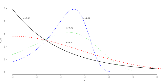
Figure 1: Inverse stable prior densities with $\rho=1$.

3 Single parameter formulation

Proposition 1. Let $\bm{X}=\left(X_{1},X_{2},\ldots,X_{n}\right)$ be a random sample from a population belonging to an exponential family of distributions with the likelihood kernel

$$L(\theta|\bm{x})\;\sim\;e^{-a\cdot\theta\;+b\;\cdot\log(\theta)},$$ (15)

where $a=a(\bm{x}),b=b(\bm{x})\in\mathbb{R}^{+}\cup\{0\},\theta=|\theta(\epsilon)|,\theta(\epsilon)\in\mathbb{R}\backslash\{0\}$. Using the non-conjugate inverse stable density $p(\theta)=IS_{\alpha,\rho}(\theta)$ as a prior for $\Theta$ yields the the proper or normalized posterior distribution

$$p(\theta|\bm{x})\;=\;\frac{e^{-a\cdot\theta\;+\;b\cdot\log(\theta)}\;IS_{\alpha,\rho}\left(\theta\right)}{\Gamma(b+1)\;\rho^{b}\;E_{\alpha,\alpha b+1}^{b+1}(-a\rho)},$$ (16)

where $\alpha$ and $\rho$ are the hyperparameters,

$$E_{\eta,\nu}^{\tau}(w)=\sum_{j=0}^{\infty}\frac{(\tau)_{j}}{j!\Gamma(\eta j+\nu)}\;w^{j}$$ (17)

is the generalized Mittag–Leffler function (Prabhakar, 1971), $\eta,\nu,\tau,w\in\mathbb{C};\Re(\eta),\Re(\nu),\Re(\tau)>0$, $(\tau)_{j}=\Gamma(\tau+j)/\Gamma(\tau)$ is the Pochammer symbol, and $(\tau)_{0}=1.$

Proof. See Appendix.

For the Poisson-gamma model in Section 1, as $b=\sum_{i=0}^{n}x_{i}\to 0$ and $\theta\to 0$, the posterior $p(\theta|\bm{x})\to\rho^{-1}/\left[\Gamma(1-\alpha)E_{\alpha,1}^{1}(-a\rho)\right]$, i.e., the limit exists. For both the gamma-gamma and inv-gamma-gamma models above, as $b=n\nu\to 0$, i.e., as $\nu\to 0,$ the posterior $p(\theta|\bm{x})\to\rho^{-1}/\left[\Gamma(1-\alpha)E_{\alpha,1}^{1}(-a\rho)\right]$ as well as $\theta\to 0$.

Corollary 1. The marginal density of the data given hyperparameters $\alpha$ and $\rho$ is

$$p(\bm{x}|\alpha,\rho)\;=\;\Gamma(b+1)\;\rho^{b}\;E_{\alpha,\alpha b+1}^{b+1}(-a\rho).$$ (18)

Proof. It is trivial and is omitted. ∎

The generalized Mittag-Leffler function in (18) above is absolutely convergent for all $a$ (see Shukla and Prajapati, 1997). If $b=0$ then we obtain the Mittag-Leffler function.

Corollary 2. The $k$th posterior moment is

$$\mathbf{E}\left(\Theta^{k}\big{|}\bm{x}\right)\;=\;\frac{\Gamma(k+b+1)\;\rho^{k}\;E_{\alpha,\alpha(k+b)+1}^{k+b+1}(-a\rho)}{\Gamma(b+1)\;E_{\alpha,\alpha b+1}^{b+1}(-a\rho)}.$$ (19)

Proof. It is trivial and thus is not provided. ∎

When $k=0$, the formula in (16) is checked as a valid probability density function.

Corollary 3. The moment generating function is straightforward to calculate as

$$\mathbf{E}\left(\exp\left(\beta\Theta\right)|\bm{x}\right)=\frac{E_{\alpha,\alpha b+1}^{b+1}(-(a-\beta)\rho)}{E_{\alpha,\alpha b+1}^{b+1}(-a\rho)}.$$ (20)

Proof. The proof follows from the property of the inverse stable distribution and is trivial.∎

Corollary 4. As $\alpha\longrightarrow 1^{-}$,

$$p(\theta|\bm{x})\;\longrightarrow\;\frac{e^{-a\cdot\theta}\;\theta^{b}\;\delta\left(\theta-\rho\right)}{e^{-a\rho}\;\rho^{b}}$$ (21)

because $E_{1^{-},(1^{-})b+1}^{b+1}(-a\rho)=e^{-a\rho}/\Gamma(b+1)$.

Proof. The proof follows from the property of the inverse stable density and is omitted. ∎

The preceding corollary suggests that the Bayes estimator $\widehat{\theta}_{Bayes}\;\big{|}_{\alpha\to 1^{-}}\;\to\;\rho$. It also indicates how $\alpha$ controls the shape and/or variability of the posterior distribution from a non-degenerate family $\left(\alpha=0^{+}\right)$ to a degenerate one $\left(\alpha=1^{-}\right)$. This shows the relevance of $\rho$ as $\widehat{\rho}\longrightarrow\theta$ when $\alpha=1^{-}$ and as $n$ goes large.

Table 1 below shows some likelihood models with their corresponding parameterizations following the above formulation and notation. The inverse stable density can also be a prior for a rate or an inverse scale parameter of two-parameter models like the inverse-Weibull, lognormal and normal-inverse densities conditional on the other parameter (see e.g. Miller, 1980; Kundu, 2008).

Table 1: Probability models with corresponding parameterizations.

Data model	Parameter $\theta$	$a$	$b$
Poisson: $\lambda^{x}e^{-\lambda}/x!$	$\lambda$	$n$	$\sum x_{i}$
Rayleigh: $\frac{x}{\sigma^{2}}\;e^{-x^{2}/(2\sigma^{2})}$	$1/\sigma^{2}$	$\sum x_{i}^{2}/2$	$n$
Half-normal: $\frac{2\sigma}{\pi}\;e^{-(x^{2}\sigma^{2})/\pi}$	$\sigma^{2}$	$\sum x_{i}^{2}/\pi$	$n/2$
Inverse Rayleigh: $(2\varepsilon^{2}/x^{3})\;e^{-\varepsilon^{2}/x^{2}}$	$\varepsilon^{2}$	$\sum 1/x_{i}^{2}$	$n$
Exponential: $\lambda e^{-\lambda x}$	$\lambda$	$\sum x_{i}$	$n$
Laplace: $(\lambda/2)\exp(-\lambda|x|)$	$\lambda$	$\sum|x_{i}|$	$n$
Inverse Exponential: $\lambda x^{-2}e^{-\lambda/x}$	$\lambda$	$\sum 1/x_{i}$	$n$
Skew-Logistic: $\lambda\left(1+e^{-x}\right)^{-\lambda-1}e^{-x}$	$\lambda$	$\sum\log\left(1+e^{-x_{i}}\right)$	$n$
Gamma: $\frac{\varepsilon^{\sigma}}{\Gamma(\sigma)}x^{\sigma-1}e^{-\varepsilon x}$	$\varepsilon,\sigma$-known	$\sum x_{i}$	$n\sigma$
Weibull: $\frac{\sigma}{\varepsilon}\left(\frac{x}{\varepsilon}\right)^{\sigma-1}e^{-(x/\varepsilon)^{\sigma}}$	$1/\varepsilon^{\sigma},\sigma$-known	$\sum x_{i}^{\sigma}$	$n$
Normal: $\frac{e^{-(x-\mu)^{2}/(2\sigma^{2})}}{\sqrt{2\pi\sigma^{2}}}$	$1/\sigma^{2},\mu$-known	$\sum(x_{i}-\mu)^{2}/2$	$n/2$
Generalized Exponential: $\varepsilon\sigma\left(1-e^{-\sigma x}\right)^{\varepsilon-1}e^{-\sigma x}$	$\varepsilon,\sigma$-known	$-\sum\log\left(1-e^{-\sigma x_{i}}\right)$	$n$

4 Estimation algorithms

4.1 Monte Carlo integration

From (90) of Appendix A, we have

$$E_{\alpha,\alpha\omega+1}^{\omega+1}(-a\rho)\;=\;\frac{1}{\rho^{\omega}\Gamma(\omega+1)}\int_{\mathbb{R}^{+}}e^{-ay}y^{\omega}\cdot IS_{\alpha,\rho}(y)dy\;\approx\;\frac{\sum_{j=1}^{J}e^{-aY_{j}}Y_{j}^{\omega}}{J\;\rho^{\omega}\;\Gamma(\omega+1)},$$ (22)

where $Y_{j}^{\prime}s\;\stackrel{{\scriptstyle ind}}{{=}}\rho S^{-\alpha}.$ Thus, the $k$th moment can be estimated using the following algorithm.

Algorithm 1

Step 1. Generate $Y_{1},Y_{2},\ldots,Y_{J}\stackrel{{\scriptstyle ind}}{{=}}\rho S^{-\alpha}.$

Step 2. Let

$$V_{\alpha,\rho,k}=\frac{\sum_{j=1}^{J}e^{-aY_{j}}Y_{j}^{b+k}}{J\;\rho^{(b+k)}\;\Gamma(k+b+1)}.$$ (23)

Step 3. Set

$$\widehat{\mathbf{E}\left(\Theta^{k}\big{|}\bm{x}\right)}=\frac{\Gamma(b+k+1)\;\rho^{k}\;V_{\alpha,\rho,k}}{\Gamma(b+1)\;V_{\alpha,\rho,0}}.$$ (24)

In particular, the Bayes estimator of $\theta$ with respect to the squared error loss criterion can be directly computed as

$$\widehat{\theta}_{1}=\frac{(b+1)\;\rho\;V_{\alpha,\rho,1}}{V_{\alpha,\rho,0}}$$ (25)

while the variance can be estimated as

$$\widehat{\mathbf{Var}\left(\Theta\big{|}\bm{x}\right)}\;=\;\frac{(b+1)\rho^{2\alpha}}{V_{\alpha,\rho,0}}\left[(b+2)V_{\alpha,\rho,2}-\frac{(b+1)\left(V_{\alpha,\rho,1}\right)^{2}}{V_{\alpha,\rho,0}}\right].$$ (26)

4.2 Posterior simulation

Let the target density be $p(\theta|\bm{x})$ and candidate density be $IS_{\alpha,\rho}(\theta),\alpha$ and $\rho$ are both known. Then

$$\frac{p(\theta|\bm{x})}{IS_{\alpha,\rho}(\theta)}\;=\;\frac{e^{-a\cdot\theta}\;\theta^{b}}{\Gamma(b+1)\;\rho^{b}\;E_{\alpha,\alpha b+1}^{b+1}(-a\rho)}.$$ (27)

The preceding expression is maximized at $\theta=b/a$ and

$$\frac{e^{-a\cdot\theta}\;\theta^{b}}{\Gamma(b+1)\;\rho^{b}\;E_{\alpha,\alpha b+1}^{b+1}(-a\rho)}\;\;<\;\;\frac{e^{-b}\;(b/a)^{b}}{\Gamma(b+1)\;\rho^{b}\;E_{\alpha,\alpha b+1}^{b+1}(-a\rho)}\;\;=\;\;Q.$$ (28)

Below is an accept-reject algorithm for generating observations from the posterior distribution (16).

Algorithm 2

Step 1. Generate $U\stackrel{{\scriptstyle d}}{{=}}U(0,1)$ and $Y\stackrel{{\scriptstyle d}}{{=}}\rho\cdot S^{-\alpha}.$

Step 2. Accept $\Theta=Y$ if

$$u<\frac{p(y|\bm{x})}{Q\cdot IS_{\alpha,\rho}(y)}\;=\;\frac{e^{-a\cdot y}\;y^{b}}{e^{-b}\;(b/a)^{b}}\;=\;e^{b-ay}\cdot\left(ay/b\right)^{b}$$ (29)

or equivalently, $\log(u)<\log\left[\frac{p(y|\bm{x})}{Q\cdot IS_{\alpha,\rho}(y)}\right]=b\;\left[\;\log(ay/b)+1\;\right]-ay;$ otherwise, go back to step 1.

Step 3. Repeat steps $1-2,B$ times and set $\widehat{\theta}_{2}=\overline{\Theta}$.

As $\alpha\to 1$, $Q=\frac{e^{-b}\;(b/a)^{b}\;}{\rho^{b}\;e^{-a\rho}}=1$ if and only if $b=a$ and $\rho=1.$ Thus, we expect high acceptance rates (close to $100\%$) of Algorithm 2 if the conditions ($\alpha\approx 1$, $b=a$ and $\rho=1$) are close to being satisfied. The same acceptance rates are to be observed for $\alpha\approx 1$, $b\neq a$ but $\rho$ is the solution of $e^{-b}\;(b/a)^{b}\;-\rho^{b}\;e^{-a\rho}=0.$

We generated 500 observations from the different posterior distributions in 1000 replications based on observed data sizes $n=15,30,60$ to test both algorithms above. We calculated the mean point estimate, the median absolute deviation (MAD) and the maximum likelihood estimates (MLE); the results are in Table 5 of Appendix B. Both algorithms are generally more precise (with smaller MAD) than the MLE, and Algorithm 2 tends to be the most precise (with the smallest MAD) for small values of $\alpha$ and the sample size. The point estimates from both algorithms are very close but can be considerably different from the MLE even for relatively large data sizes. It is observed that both bias and variability decrease as the sample size increases in all cases as expected.

5 Predictive distributions

Consider the exponential data model

$$f(x|\theta)\;=\;c\cdot e^{-a\cdot\theta\;+\;b\cdot\log(\theta)},$$ (30)

where $a=a(x),b=b(x),c=c(x)\in\mathbb{R}^{+}.$ The prior predictive distribution of a conditionally independent new observation $x^{*}$ is

$$p(x^{*})\;=\;\int_{\theta}f(x^{*}|\theta)\cdot IS_{\alpha,\rho}(\theta)d\theta\;\sim\;c^{*}\;\Gamma(b^{*}+1)\;\rho^{b^{*}}\;E_{\alpha,\alpha b^{*}+1}^{b^{*}+1}(-a^{*}\rho),$$ (31)

where $a^{*}=a(x^{*})$, $b^{*}=b(x^{*})$, and $c^{*}=c(x^{*})$ is an appropriate normalizing constant or function. We now propose a class of prior predictive densities for a family of transformations $a(X^{*})$ that provides a way of simulating $X^{*}$ by generating $A^{*}$ or inverting $a(X^{*})$, and hence allows testing of prior beliefs. Note that these predictive distributions can be easily plotted using the maximum likelihood estimates of the hyperparameters and the Monte Carlo approximation (22).

Proposition 2. Let $b$ and $c$ be free of $x$ (see Table 1) and $X^{*}\to a(X^{*})=A^{*}$ be a one-to-one mapping and invertible. Then the prior predictive density of $A^{*}$ is

$$p(a^{*})\;=\;b\;\rho\;\Gamma(1+\alpha(b-1))\;E_{\alpha,\alpha b+1}^{b+1}(-a^{*}\rho).$$ (32)

Proof. The proof follows from the well-known Mellin transform of the generalized Mittag-Leffler function (Shukla and Prajapati, 1997) below for $z=1,\eta=\alpha,\nu=\alpha b+1,\tau=b+1$ as

$$\int_{\mathbb{R}^{+}}w^{z-1}\;E_{\eta,\nu}^{\tau}(-\rho w)\;dw=\frac{\Gamma(z)\;\Gamma(\tau-z)}{\Gamma(\tau)\;\rho^{z}\;\Gamma(\nu-z\eta)}.$$ (33)

∎

The above family of proper density functions can easily be plotted using the approximation in (22).

Corollary 5. The $k$th moment can be calculated using formula (33) as

$$\mathbf{E}\left(A^{*}\right)^{k}\;=\;\frac{\Gamma(\alpha b+1-\alpha)\;\Gamma(k+1)\;\Gamma(b+1-(k+1))}{\Gamma(b)\;\rho^{k}\;\Gamma(\alpha b+1-(k+1)\alpha)}.$$ (34)

Proof. It is trivial and is omitted. ∎

Formula (32) can be checked to be proper when $k=0$ in the preceding corollary. The $k$th moment exists provided $b>k$.

Example 1. Let $f(x|\theta)=\theta\exp(-\theta x),\in\mathbb{R}^{+}.$ Then $a^{*}=x^{*},b=1,$ and thus,

$$p(a^{*})\;=\;\rho\;E_{\alpha,\alpha+1}^{2}(-x^{*}\rho),\quad\text{and}\quad\mathbf{E}\left(A^{*}\right)^{k}\;=\;\mathbf{E}\left(X^{*}\right)^{k}\;=\;\frac{\Gamma(k+1)\;\Gamma(1-k)}{\rho^{k}\Gamma(1-\alpha k)},\;\;k\notin\mathbb{N}^{+}.$$ (35)

Example 2. Let $f(x|\theta)\sim\theta^{1/2}\exp\left(-\theta x^{2}\right),x\in\mathbb{R}$. Then $a^{*}=x*^{2},b=1/2,$ and therefore,

$$p(a^{*})\;=\;\rho^{1/2}\;(1/2)\;E_{\alpha,\alpha/2+1}^{3/2}(-a^{*}\rho);\;\;\mathbf{E}\left(A^{*}\right)^{k}=\mathbf{E}\left(X^{*}\right)^{2k}=\frac{\Gamma(1-k)\;\Gamma(k+1/2)}{\sqrt{\pi}\;\Gamma(1-\alpha k)\;\rho^{k}},\;k\notin\mathbb{N}^{+}.$$ (36)

When $k=0$, the preceding $p(a^{*})$’s are easily checked as proper prior predictive density functions.

After observing the data $\bm{x}\in\mathbb{R}^{n}$, the posterior predictive distribution of a conditionally independent new observation $A^{*}=a(X^{*})$ is

$$p(a^{*}|\bm{x})\;=\;\int_{\theta}f(a^{*}|\theta,\bm{x})p(\theta|\bm{x})d\theta\;\sim\;c^{*}\;\rho^{b^{*}}E_{\alpha,\alpha b^{\prime}+1}^{b^{\prime}+1}\left(-(a+a^{*})\rho\right),\qquad b^{\prime}=b^{*}+b,$$ (37)

where $a=a(\bm{x}),b^{\prime}\in\mathbb{R}^{+},b\text{ and $b^{*}$-both known and free of}\;x\;(\text{like most of the examples in Table \ref{t1}}),$ and $c^{*}=c(x^{*})\in\mathbb{R}^{+}$ is some normalizing function or constant.

Example 3. Let $f(x|\theta)=\theta\exp(-\theta x),x\in\mathbb{R}^{+}.$ Then $a^{*}=x^{*},b^{*}=1,a=\sum x_{i},b=n,$ and thus,

$$p(a^{*}|\bm{x})\;\sim\;\rho\;E_{\alpha,\alpha(n+1)+1}^{n+2}(-(a+a^{*})\rho).$$ (38)

Example 4. Let $f(x|\theta)\sim\theta^{1/2}\exp\left(-\theta x^{2}\right),x\in\mathbb{R}$. Then $a^{*}=x*^{2},b^{*}=1/2,a=\sum x_{i}^{2},b=n/2$ and hence,

$$p(a^{*}|\bm{x})\;\sim\;\rho^{1/2}\;E_{\alpha,\alpha(n+1)/2+1}^{(n+1)/2+1}(-(a+a^{*})\rho).$$ (39)

The above posterior predictive distributions can directly be plotted using (22) also.

6 Hierarchical models

Recall that $p(\lambda|data)\sim p(data|\lambda)\cdot p(\lambda)$, where the marginal prior $p(\lambda)\sim\int p(\lambda|\theta)IS_{\alpha,\rho}(\theta)d\theta\sim\int\exp(-g(\lambda)\cdot\theta)\theta^{b}IS_{\alpha,\rho}(\theta)d\theta\sim E_{\alpha,\alpha b+1}^{b+1}(-g(\lambda)\cdot\rho)$ follows from Corollary 1, with the inverse stable density as the mixing distribution. The marginal prior family can be plotted using the Monte Carlo algorithm above and can be made proper using the Mellin transform property (33). Below are some applications of the inverse stable prior in hierarchical contexts.

Normal-normal model

Let $\theta$ be the inverse variance and consider

$$\overline{X}\;|\;\lambda\stackrel{{\scriptstyle d}}{{=}}N(\lambda,1/n),\quad\Lambda\;|\;\theta\stackrel{{\scriptstyle d}}{{=}}N\left(0,\;\theta^{-1}\right),\quad\theta\stackrel{{\scriptstyle d}}{{=}}IS_{\alpha,\rho}\left(\theta\right),\;\;\;\;\alpha,\rho\text{-known.}$$ (40)

The marginal prior of $\Lambda$ can be shown as

$$p(\lambda)\;\sim\;\;\rho^{1/2}\;E_{\alpha,\alpha/2+1}^{1/2+1}(-\lambda^{2}\rho/2).$$ (41)

Also, the hyperparameters $\alpha$ and $\rho$ can be estimated by maximizing

$$data\;|\;\alpha,\rho\;\sim\;\mathbf{E}_{\Theta}\left[\left(2\pi\frac{n+\Theta}{n\Theta}\right)^{-1/2}\exp\left(-\frac{n\Theta\overline{x}^{2}}{2(n+\Theta)}\right)\right].$$ (42)

The Gibbs sampler for this model can be performed as

$$\Lambda\;|\;data,\theta\;\stackrel{{\scriptstyle d}}{{=}}\;N\left(\frac{\overline{x}}{1+\theta/n}\;,\;\left(n+\theta\right)^{-1}\right),$$ (43)

and

$$\Theta\;|\;\lambda,data\;\sim\;\theta^{1/2}\exp\left(-\frac{\lambda^{2}}{2}\theta\right)\cdot IS_{\alpha,\rho}\left(\theta\right).$$ (44)

Poisson-exponential model

Let

$$data\;|\;\lambda\stackrel{{\scriptstyle d}}{{=}}{\tt Poisson}(\lambda),\quad\Lambda\;|\;\theta\stackrel{{\scriptstyle d}}{{=}}\theta e^{-\lambda\theta},\quad\Theta\stackrel{{\scriptstyle d}}{{=}}IS_{\alpha,\rho}\left(\theta\right),\;\;\;\alpha,\rho\text{-known.}$$ (45)

The marginal prior of $\Lambda$ can be obtained as

$$p(\lambda)\;\sim\;\;\rho\;E_{\alpha,\alpha+1}^{2}\left(-\rho\lambda\right).$$ (46)

Moreover, maximizing

$$data\;|\;\alpha,\rho\;\sim\;\mathbf{E}_{\Theta}\left[\frac{\Gamma\left(\sum_{j=1}^{n}x_{j}+1\right)}{\left(n+\Theta\right)^{\sum_{j=1}^{n}x_{j}+1}\;\prod_{j=1}^{n}x_{j}}\right]$$ (47)

gives estimates of the hyperparameters $\alpha$ and $\rho.$ The Gibbs sampler for this model can be accomplished as

$$\Lambda\;|\;data,\theta\;\stackrel{{\scriptstyle d}}{{=}}\;{\tt Gamma}\left(\sum_{j=1}^{n}x_{j}+1\;,\;n+\theta\right),$$ (48)

and

$$\Theta\;|\;\lambda,data\;\sim\;\theta\exp\left(-\lambda\theta\right)\cdot IS_{\alpha,\rho}\left(\theta\right).$$ (49)

Poisson-exponential with unequal intensity rates

Let

$$X_{i}\;|\;\lambda_{i}\stackrel{{\scriptstyle d}}{{=}}{\tt Poisson}(\lambda_{i}),\quad\Lambda_{i}\;|\;\theta\stackrel{{\scriptstyle d}}{{=}}\theta e^{-\lambda_{i}\theta},\quad\Theta\stackrel{{\scriptstyle d}}{{=}}IS_{\alpha}\left(\theta\right)\;=\;IS_{\alpha,1}\left(\theta\right),\;\;\;\alpha\text{-known}.$$ (50)

The marginal prior of $\bm{\Lambda}=\left(\Lambda_{1},\Lambda_{2},\ldots,\Lambda_{n}\right)^{\prime}$ can be calculated as

$$p(\bm{\lambda})\;\sim\;E_{\alpha,\alpha n+1}^{n+1}\left(-\sum_{i=1}^{n}\lambda_{i}\right),\qquad\bm{\lambda}=(\lambda_{1},\lambda_{2},\ldots,\lambda_{n})^{\prime}.$$ (51)

Then

$$\Lambda_{i}\;|\;data,\theta\;\stackrel{{\scriptstyle d}}{{=}}\;{\tt Gamma}\left(x_{i}+1\;,\;1+\theta\right),$$ (52)

and

$$\mathbf{E}\left(\Lambda_{i}\;|\;data,\theta\right)\;=\;(x_{i}+1)/(1+\theta)=(1-\kappa)x_{i}+\frac{1}{\theta}\kappa,$$ (53)

where $\kappa=\theta/(1+\theta)$ describes the shrinkage. Hence,

$$\mathbf{E}\left(\Lambda_{i}\;|\;data\right)\;=\;(x_{i}+1)\mathbf{E}_{\Theta|data}[(1+\theta)^{-1}],$$ (54)

where

$$\Theta\;|\;data\;\stackrel{{\scriptstyle d}}{{=}}K\;\left(\frac{1}{1+\theta}\right)^{\sum_{j=1}^{n}x_{j}}\left(1-\frac{1}{1+\theta}\right)^{n}IS_{\alpha}(\theta)=K\;\left(1-\kappa\right)^{\sum_{j=1}^{n}x_{j}}\kappa^{n}\;IS_{\alpha}(\theta).$$ (55)

The normalizing constant $K$ can be straightforwardly calculated using Monte Carlo integration. Therefore,

$$\mathbf{E}\left(\Lambda_{i}\;|\;data\right)=(x_{i}+1)\cdot\mathbf{E}_{\Theta}\left[K\;\left(1-\kappa\right)^{\sum_{j=1}^{n}x_{j}+1}\kappa^{n}\right].$$ (56)

Global shrinkage in normal-normal model

Let $\theta$ be the inverse variance. Consider

$$X_{i}\;|\;\lambda_{i}\stackrel{{\scriptstyle d}}{{=}}N(\lambda_{i},1),\quad\Lambda_{i}\;|\;\theta\stackrel{{\scriptstyle d}}{{=}}N(0,\theta^{-1}),\quad\Theta\stackrel{{\scriptstyle d}}{{=}}IS_{\alpha}\left(\theta\right),\;\;\alpha\text{-known}.$$ (57)

The marginal prior for $\bm{\Lambda}$ is

$$p(\bm{\lambda})\;\sim\;E_{\alpha,\alpha n/2+1}^{n/2+1}\left(-||\bm{\lambda}||_{2}^{2}/2\right).$$ (58)

Then

$$\Lambda_{i}\;|\;data,\theta\;\stackrel{{\scriptstyle d}}{{=}}\;N\left(\frac{x_{i}}{1+\theta}\;,\;\frac{1}{1+\theta}\right),$$ (59)

and

$$\mathbf{E}\left(\Lambda_{i}\;|\;data,\theta\right)\;=\;x_{i}/(1+\theta)=(1-\kappa)x_{i},$$ (60)

where $\kappa=\theta/(1+\theta).$ Hence,

$$\mathbf{E}\left(\Lambda_{i}\;|\;data\right)\;=\;x_{i}\cdot\mathbf{E}_{\Theta|data}[(1+\theta)^{-1}],$$ (61)

where

$$\Theta\;|\;data\; \stackrel{{\scriptstyle d}}{{=}} K\;\left(\frac{1}{1+\theta}\right)^{n/2}\exp\left(||\bm{x}||_{2}^{2}/[2(1+\theta)]\right)\;\theta^{n/2}\;IS_{\alpha}(\theta)$$ (62)

$$= K\;\kappa^{n/2}\exp\left((1-\kappa)||\bm{x}||_{2}^{2}/2\right)\;IS_{\alpha}(\theta).$$ (63)

Thus,

$$\mathbf{E}\left(\Lambda_{i}\;|\;data\right)=x_{i}\cdot\left(1-\mathbf{E}_{\Theta}\left[K\;\kappa^{n/2+1}\exp\left((1-\kappa)||\bm{x}||_{2}^{2}/2\right)\;\right]\right).$$ (64)

The implied density for $\kappa$ is $p(\kappa)\sim\left(1-\kappa\right)^{-2}\cdot IS_{\alpha}\left(\frac{\kappa}{1-\kappa}\right)$ (see also Polson and Scott, 2012a). The effect of $\alpha$ on the density of $\kappa$ is shown in the figure below. The density converges to dirac measure at $\kappa=1/2$ as $\alpha\to 1^{-}$ and $p(\kappa)\sim 1/\Gamma(1-\alpha)$ as $\kappa\to 0^{+}.$ From Figure 2, the density $p(\kappa)$ is bounded at both endpoints $(\kappa=0\;\text{or}\;\theta=0\;;\;\kappa=1\;\text{or}\;\theta=\infty)$

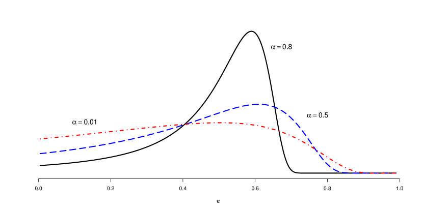
Figure 2: Marginal prior densities of $\kappa$ as a function of $\alpha$.

If we consider the normal scale mixture in application 4 of section 1, then it can be shown that

$$\mathbf{E}\left(\Lambda_{i}\;|\;data\right)=x_{i}\cdot\left[1-\mathbf{E}_{\delta^{2}|data}\;\left(\kappa^{\prime}|\;data\;\right)\right]$$ (65)

where $\kappa^{\prime}=1/(1+\delta^{2}).$

We compare the two priors in terms of their observed frequentist risks ($L_{1}$- and squared $L_{2}$- norms). We generated 1000 data samples following these five setups:

Case I: $\Lambda_{i}\sim N(0,1)$ and $X_{i}\;|\;\lambda_{i}\sim N(\lambda_{i},1),\;i=1,\ldots,9.$

Case II: $\Lambda_{1},\Lambda_{2},\Lambda_{3}\sim N(0,1);$ $X_{1:3}\;|\;\lambda_{1}\sim N(\lambda_{1},1),X_{4:6}\;|\;\lambda_{2}\sim N(\lambda_{2},1),X_{7:9}\;|\;\lambda_{3}\sim N(\lambda_{3},1).$

Case III: $\Lambda_{1},\Lambda_{2},\Lambda_{3}\sim N(0,100);$ $X_{1:3}\;|\;\lambda_{1}\sim N(\lambda_{1},1),X_{4:6}\;|\;\lambda_{2}\sim N(\lambda_{2},1),X_{7:9}\;|\;\lambda_{3}\sim N(\lambda_{3},1).$

Case IV: $X_{i}\sim N(\lambda_{i},1),\;\Lambda_{i}\sim 0.1\times t(df=2,\;scale=3)+0.9\times\delta_{0}$ where $\delta_{0}$ is the Dirac measure at zero; $i=1,\ldots,250.$

Case V: $X_{i}\sim N(\lambda_{i},1.5),\;\Lambda_{i}\sim 0.1\times t(df=2,\;scale=3)+0.9\times\delta_{0};i=1,\ldots,250.$

Table 2 summarizes the results over the 1000 samples. For each of the five cases and procedures (inverted beta, inverse stable with $\alpha=0.01,0.5,0.99$) we present

$$\frac{\sum_{j=1}^{1000}\sum_{i=1}^{n}|\lambda_{ji}-\hat{\lambda}_{ji}|^{k}}{1000},\qquad k=1,2,$$ (66)

where $\lambda_{ji}$s are the selected values used for comparison with the posterior means, and $n$ is the number of $\lambda_{i}$s for that case. Overall, the results are similar for both priors, suggesting the value of further investigation of the inverse stable family of priors as an alternative to the inverse beta. In terms of the $L_{1}$ risk, we are able to find $\alpha$’s where the inverse stable provides a prior at least as good as the inverse beta. For the squared $L_{2}$ risk, the two priors give similar results for Cases I, II, and V. Note that the posteriors were standardized using numerical (inverted beta) and Monte Carlo methods. We subjected $2\times 10^{7}$ random numbers for acceptance or rejection in our simulations.

Table 2: Mean $L_{1}$ and squared $L_{2}$ risks.

$L_{1}$ Squared $L_{2}$ Inv Beta Inv Stable Inv Beta Inv Stable $\alpha=0.01$ $\alpha=0.5$ $\alpha=0.99$ $\alpha=0.01$ $\alpha=0.5$ $\alpha=0.99$ Case I 6.247 6.010 6.046 6.147 6.721 6.226 6.284 6.425 Case II 7.386 7.642 7.567 7.546 10.655 11.217 10.952 10.520 Case III 66.787 65.768 66.118 66.085 1068.171 981.817 993.494 993.166 Case IV 158.674 156.490 156.378 155.814 181.981 201.705 201.712 202.071 Case V 245.558 235.482 235.386 234.689 386.416 389.802 389.568 387.966

For several data sets, we have plotted in Figure 3 the likelihood of $\delta^{2}$ based on (6) against the inverted beta prior in (7) .

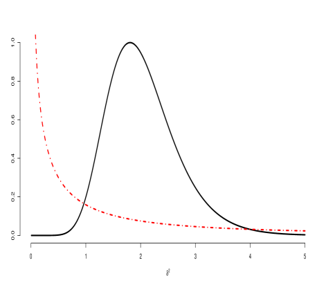
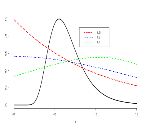
Figure 3: The solid black lines show the likelihoods as a function of $\delta^{2}$ and $\theta$, respectively. (Left) The solid black line shows the likelihood as a function of $\delta^{2}$ together with the inverted beta prior. (Right) The black line represents the likelihood as a function of $\theta$ together with the inverse stable priors for $\alpha=0.01(red),0.5(blue),0.7(green).$

As expected, the inverted beta priors are usually informative. That is, the prior density has appreciable mass where the likelihood is negligible, typically for small values of $\delta^{2}.$ The corresponding plots of the likelihood of $\theta$ against the inverse stable prior in (57) have much better behavior. Fifty data points were generated from $N\left(0,\;1.5^{2}\right)$ and the corresponding likelihoods were normalized to obtain a maximum of one.

Local shrinkage in normal-normal model

Let $\theta_{i}$ be the local inverse variance. When $\Lambda_{i}\;|\;\theta_{i}\stackrel{{\scriptstyle d}}{{=}}N\left(0,\theta_{i}^{-1}\right)$ and $\Theta_{i}\;\stackrel{{\scriptstyle d}}{{=}}IS_{\alpha}(\theta_{i})$ above, then the marginal prior for $\Lambda_{i}$ is

$$p(\lambda_{i})\;\sim\;E_{\alpha,\alpha/2+1}^{1/2+1}\left(-\lambda_{i}^{2}/2\right).$$ (67)

Furthermore,

$$\Lambda_{i}\;|\;x_{i},\theta_{i}\;\stackrel{{\scriptstyle d}}{{=}}\;N\left(\frac{x_{i}}{1+\theta_{i}}\;,\;\frac{1}{1+\theta_{i}}\right),$$ (68)

and

$$\mathbf{E}\left(\Lambda_{i}\;|\;x_{i},\theta_{i}\right)\;=\;x_{i}/(1+\theta_{i})=(1-\kappa_{i})x_{i},\qquad\kappa_{i}=\theta_{i}/(1+\theta_{i}).$$ (69)

Therefore,

$$\mathbf{E}\left(\Lambda_{i}\;|\;x_{i}\right)\;=\;x_{i}\cdot\mathbf{E}_{\Theta_{i}|x_{i}}[(1+\theta_{i})^{-1}],$$ (70)

where

$$\Theta_{i}\;|\;x_{i}\; \stackrel{{\scriptstyle d}}{{=}} K\;\left(\frac{1}{1+\theta_{i}}\right)^{1/2}\exp\left(x_{i}^{2}/[2(1+\theta_{i})]\right)\;IS_{\alpha}(\theta_{i})\;\theta_{i}^{1/2}$$ (71)

$$= K\;\kappa_{i}^{1/2}\exp\left((1-\kappa_{i})x_{i}^{2}/2\right)\;IS_{\alpha}(\theta_{i}).$$ (72)

Hence,

$$\mathbf{E}\left(\Lambda_{i}\;|\;x_{i}\right)=x_{i}\cdot\left(1-\mathbf{E}_{\Theta_{i}}\left[K\;\kappa_{i}^{1/2+1}\exp\left((1-\kappa_{i})x_{i}^{2}/2\right)\right]\right).$$ (73)

7 Real data illustration

We considered the Quine data (available in the MCMCpack package of R). The Quine dataset has $n=146$ children from Walgett, New South Wales, Australia, who were classified by culture, age, sex and learner status, and the number of days absent ($X_{j}$’s) from school in a particular school year was recorded. We applied the hierarchical model below only to the number of days absent:

$$X_{j}\;|\;\lambda \sim \;{\tt Poisson}(\lambda),$$ (74)

$$\Lambda\;|\;\theta \sim \;\theta e^{-\lambda\theta},$$ (75)

$$\Theta\;|\;\alpha,\rho\; \sim \;IS_{\alpha,\rho}(\theta),$$ (76)

$$(\alpha,\rho)\; \sim \;h(\alpha)\;g_{\alpha}(\rho),$$ (77)

where $h(\cdot)$ is a well-defined function in $(0,1)$ and $g_{\alpha}(\rho)$ is the heavy-tailed (with infinite mean) $\sqrt{\alpha}^{\;+}$-stable hyperprior in $\mathbb{R}^{+}.$ Note that we allow dependence between hyperparameters. Moreover, $\sum_{j=1}^{n}X_{j}=W\stackrel{{\scriptstyle d}}{{=}}{\tt Poisson}(n\lambda)$ and

$$W\;\big{|}\;\alpha,\rho\; \sim \;\int\left[\int\frac{e^{-n\lambda}(n\lambda)^{w}}{w!}\cdot\theta e^{-\lambda\theta}\cdot IS_{\sqrt{\alpha},\rho^{-\alpha}}(\theta)\;d\lambda\right]\;d\theta$$ (78)

$$= \;\int\left[\int\frac{n^{w}\;e^{-(n+\theta)\lambda}\lambda^{w}}{w!}\;d\lambda\right]\theta\cdot IS_{\sqrt{\alpha},\rho^{-\alpha}}(\theta)\;d\theta$$ (79)

$$= \;\mathbf{E}_{\Theta}\left[\frac{\Theta\;n^{w}}{(n+\Theta)^{w+1}}\right].$$ (80)

A simple grid search (or any other optimization method) can straightforwardly be applied to (80) to find the maximum likelihood estimates of the hyperparameters using (22). Observe that the parameter $\alpha$ is bounded in $(0,1)$, making the maximum likelihood search relatively fast.

Let $\eta=(\alpha,\rho)$. Then a Gibbs sampler consists of the following:

$$\Lambda\;|\;\theta,w,\eta\; \sim \;\Gamma(w+1,n+\theta),$$

$$\Theta\;|\;\lambda,w,\eta\; \sim \;\theta e^{-\lambda\theta}IS_{\alpha,\rho}(\theta),$$

$$\eta\;|\;\lambda,w,\theta\; \sim \;IS_{\alpha,\rho}(\theta)h(\alpha)g_{\alpha}(\rho).$$

Using a non-informative prior $h(\alpha)=1,$ we generated 13000 joint posterior samples with 3000 observations as burn-ins. Note that $g_{\alpha}(\rho)$ is heavy-tailed where the mean is non-existent (see Bhadra et al., 2016, and the references therein for robustness). Furthermore, samples from the first two conditional distributions of the Gibbs sampler above can directly be obtained using a built-in function (in R, for example) and Algorithm 2, correspondingly. We utilized a grid-based method to sample from $(\eta\;|\;\lambda,w,\theta)$ using at least 30000 equally spaced (marginally) $(\alpha,\rho)$ values from $(0.01,0.99)\times(0.005,3)$ as grids. In this process, we evaluated $IS_{\alpha,\rho}(\theta)h(\alpha)g_{\alpha}(\rho)$ using the following widely used integral formula:

$$g_{\alpha}(s)=\frac{\alpha s^{1/(\alpha-1)}}{\pi(1-\alpha)}\int\limits_{-\pi/2}^{\pi/2}\exp\left\{-s^{\alpha/(\alpha-1)}U(\phi;\alpha)\right\}U(\phi;\alpha)d\phi,$$ (81)

where

$$U(\phi;\alpha)=\left[\frac{\sin(\alpha(\phi+\pi/2))}{\cos\phi}\right]^{\alpha/({\alpha-1})}\frac{\cos\left((\alpha-1)\phi+\alpha\pi/2\right)}{\cos\phi},$$ (82)

and normalized the values by their sum to form the weights used in sampling.

The simulated posterior fit of $(\Lambda,\Theta^{-1})$ (means) is in Figure 4.

Figure 4: Joint posterior fit of $(\Lambda,\Theta^{-1}).$

The point estimates and highest posterior density (HPD) credible intervals for $\lambda$ and $\theta^{-1}$ are in Table 3. Note that the HPDinterval function from the lme4 package of R was utilized for this exercise. The point estimates and the 95% HPD credible intervals for the Poisson rate $\lambda$ tend to cluster around $16.456$ and $(15.796\;,17.108)$, respectively. The posterior distribution of $\theta^{-1}$ is right-skewed where estimates range from 1.921 to 116.488. Notice that the estimates for $\theta$ are easily obtained as the reciprocals of the point estimate and credible interval for $\theta^{-1}$.

Table 3: Point estimates and 95% HPD credible intervals for the Quine data.

$\lambda$ $\theta^{-1}$ Point Interval Point Interval 16.456 (15.796 , 17.108) 32.748 (1.921 , 116.488)

Moreover, the point estimates and credible intervals for $\alpha$ and $\rho$ are in Table 4. The point estimates and the 95% HPD credible intervals for $\alpha$ tend to cluster around $0.409$ and $(0.049\;,0.804)$, respectively. The estimates of $\rho$ range from 0.005 to 1.184. These results are made apparent by the posterior plot of $(\eta\;|\;\lambda,w,\theta)$ in Figure 5 .

Table 4: Point estimates and 95% HPD credible intervals for $\alpha$ and $\rho$.

$\alpha$ $\rho$ Point Interval Point Interval 0.409 (0.049 , 0.804) 0.351 (0.005 , 1.184)

Figure 5: Posterior of $(\alpha,\rho).$

8 Concluding points

We propose a family of proper and non-conjugate priors for an array of discrete and continuous exponential probability models. The resulting posterior family is proper. The normalized posterior family then allows for the derivation of some properties such as the moment generating function, which leads to the closed-form formulas of the moments including the Bayes estimator with respect to the quadratic loss criterion. The posterior class ranges from a non-degenerate to a degenerate family of distributions. The parameter $\alpha\in(0,\;1)$ modulates the shapes of the posterior distribution that adapts to a large class of signal patterns. We develop algorithms for calculating the Bayes point and interval estimates (under the squared error loss) and for generating samples from the posterior distributions. We illustrate the proposed methodology using a real data set and extend it to the hierarchical settings. In particular, we show that inverse stable can provide better shrinkage than the inverted beta prior for the normal-normal model with a global variance. We also introduce a hyperprior density of the form $h(\alpha)g_{\alpha}(\rho).$

From (22) and Corollary 1, maximum likelihood search can be made faster by the boundedness of the parameter $\alpha$. If $p(data|\alpha,\rho)\sim\int\int p(data|\lambda)p(\lambda|\theta)IS_{\alpha,\rho}(\theta)d\theta d\lambda$ is well-behaved then point estimates of the hyperparameters are easily obtainable.

Note that it is straightforward to specify a heavy-tailed prior for $\Theta$. Without loss of generality, let $\rho=1$ and

$$\Theta\;\sim\;\theta^{-1-\alpha^{\prime}/\alpha}\cdot IS_{\alpha}\left(\theta\right),$$ (83)

where $0<\alpha\leq\alpha^{\prime}<1.$ By simple substitution, it is easy to show that the mean of $\Theta$ fails to exist in this case. From Proposition 1,

$$p(\theta|\bm{x})\;=\;\frac{e^{-a\cdot\theta\;+\;b^{\prime}\cdot\log(\theta)}\;IS_{\alpha}\left(\theta\right)}{\Gamma(b^{\prime}+1)\;\rho^{b^{\prime}}\;E_{\alpha,\alpha b^{\prime}+1}^{b^{\prime}+1}(-a\rho)},$$ (84)

where $b^{\prime}=b-(\alpha+\alpha^{\prime})/\alpha\geq 0.$ This suggests that the heavy-tailed specification is valid only for $b\geq 2$ as $(\alpha+\alpha^{\prime})/\alpha\geq 2.$ Clearly, $\alpha^{\prime}=\alpha$ is a straightforward choice. This formulation achieves Bayesian ‘robustness’ in the sense of Bhadra et al. (2016) and the references therein.

The inverse stable prior is worth a more extensive investigation. The following are specific worthy explorations for the future: the extensive comparison of the inverse stable prior with existing priors (e.g., inverted beta) for rate or inverse scale (e.g., $\delta$ vs. $\theta^{-0.5}$) or inverse variance parameter under different practical settings and/or criteria; the mitigation of hypothesis testing procedures and hyper/prior sensitivity analysis; the investigation of the acceptance rates of Algorithm 2 for small $\alpha$ values; the specification of $h(\alpha)$ and application of the hyperprior density in different settings especially concerning predictive distributions; and the development of sound inference procedures for more general hierarchical models especially involving the heavy-tailed prior (83), i.e., with $0<\alpha^{\prime}<1.$

9 References

10 Appendix A: Proof of Proposition 1

The posterior distribution kernel can be written as

$$L(\theta|\bm{x})\cdot IS_{\alpha,\rho}(\theta)\;\sim\;e^{-a\cdot\theta}\;\theta^{b}\cdot\frac{\rho^{1/\alpha}\;\theta^{-1-1/\alpha}}{\alpha}\;g_{\alpha}\left(\;\rho^{1/\alpha}\theta^{-1/\alpha}\;\right)$$ (85)

where $\alpha$ and $\rho$ are the hyperparameters. To determine the normalizing constant,

$$\int_{\mathbb{R}^{+}}e^{-a\cdot\theta}\;\theta^{b}\cdot\frac{\rho^{1/\alpha}\;\theta^{-1-1/\alpha}}{\alpha}\;g_{\alpha}\left(\;\rho^{1/\alpha}\;\theta^{-1/\alpha}\;\right)d\theta\quad \stackrel{{\scriptstyle u=\rho^{1/\alpha}\theta^{-1/\alpha}}}{{=}}\quad\int_{\mathbb{R}^{+}}e^{-a\rho u^{-\alpha}}\;\left(\rho u^{-\alpha}\right)^{b}\;g_{\alpha}\left(u\right)du$$ (86)

$$=\sum_{j=0}^{\infty}\frac{(-a\rho)^{j}}{j!}\;\rho^{b}\left(\int_{\mathbb{R}^{+}}u^{-\alpha(j+b)}\;g_{\alpha}\left(u\right)du\right).$$ (87)

Using the Mellin transform formula for the $\alpha^{+}$-stable density (Zolotarev, 1986),

$$\sum_{j=0}^{\infty}\frac{(-a\rho)^{j}}{j!}\;\rho^{b}\left(\int_{\mathbb{R}^{+}}u^{-\alpha(j+b)}\;g_{\alpha}\left(u\right)du\right) =\sum_{j=0}^{\infty}\frac{(-a\rho)^{j}}{j!}\;\rho^{b}\left(\frac{\Gamma(1+j+b)}{\Gamma(1+\alpha(j+b))}\right)$$ (88)

$$=\left(\rho^{b}\;\Gamma(b+1)\right)\;\sum_{j=0}^{\infty}\frac{(-a\rho)^{j}(b+1)_{j}}{j!\Gamma(\alpha j+\alpha b+1)}$$ (89)

$$=\left(\Gamma(b+1)\;\rho^{b}\right)\cdot E_{\alpha,\alpha b+1}^{b+1}(-a\rho).\qed$$ (90)

11 Appendix B: Test results

Table 5: Means and MAD of estimates.

Data model $(\alpha,\rho)$ Method $n=15$ $n=30$ $n=60$ Ave MAD Ave MAD Ave MAD Poisson$(\theta=4)$ $(0.4,4)$ $\widehat{\theta_{1}}$ 3.995 0.513 4.012 0.345 3.992 0.253 $\widehat{\theta_{2}}$ 3.996 0.508 4.009 0.359 3.992 0.258 MLE 3.972 0.494 3.999 0.346 3.986 0.247 Rayleigh$\left(\sigma=\sqrt{2/\pi}\right)$ $\left(0.5,1\right)$ $\widehat{\theta_{1}}$ 1.322 0.303 1.303 0.230 1.271 0.150 $\widehat{\theta_{2}}$ 1.322 0.297 1.304 0.228 1.271 0.150 MLE 1.332 0.330 1.301 0.236 1.268 0.155 Half-normal $\left(\sigma=\sqrt{\pi/2}\right)$ $(0.6,\sqrt{2/\pi})$ $\widehat{\theta_{1}}$ 1.401 0.285 1.492 0.261 1.540 0.242 $\widehat{\theta_{2}}$ 1.401 0.289 1.493 0.265 1.540 0.242 MLE 1.815 0.606 1.684 0.408 1.629 0.299 Generalized Exponential $(\theta=2)$ $(0.8,1.5)$ $\widehat{\theta_{1}}$ 2.003 0.296 2.031 0.276 2.026 0.220 $\widehat{\theta_{2}}$ 2.003 0.303 2.032 0.267 2.026 0.222 MLE 2.164 0.522 2.084 0.367 2.034 0.253 Exponential $(\theta=1)$ $(0.95,1)$ $\widehat{\theta_{1}}$ 1.051 0.066 1.054 0.073 1.046 0.079 $\widehat{\theta_{2}}$ 1.051 0.065 1.054 0.072 1.046 0.081 MLE 1.061 0.241 1.035 0.181 1.011 0.125