Collinear Spin-density-wave Order and Anisotropic Spin Fluctuations
in the Frustrated $J_{1}$–$J_{2}$ Chain Magnet $\mathrm{NaCuMoO_{4}(OH)}$

Abstract

The phase diagram of the quasi-one-dimensional magnet $\mathrm{NaCuMoO_{4}(OH)}$ is established through single-crystal NMR and heat-capacity measurements. The ²³Na and ¹H NMR experiments indicate a spiral and a collinear spin-density-wave (SDW) order below and above $B_{c}$ = 1.5-1.8 T, respectively. Moreover, in the paramagnetic state above the SDW transition temperature, the nuclear spin-lattice relaxation rate $1/T_{1}$ indicates anisotropic spin fluctuations that have gapped excitations in the transverse spectrum but gapless ones in the longitudinal spectrum. These static and dynamic properties are well described by a theoretical model assuming quasi-one-dimensional chains with competing ferromagnetic nearest-neighbor interactions $J_{1}$ and antiferromagnetic next-nearest-neighbor interactions $J_{2}$ ($J_{1}$–$J_{2}$ chains). Because of the excellent crystal quality and good one dimensionality, $\mathrm{NaCuMoO_{4}(OH)}$ is a promising compound to elucidate the unique physics of the frustrated $J_{1}$–$J_{2}$ chain.

I Introduction

Frustrated magnets with competing magnetic interactions are expected to exhibit exotic ground states such as spin liquids SL ; SL2 ; SL3 , valence bond solids SL2 ; VBC , and spin nematic states nematic ; nematic2 ; nematic3 ; 1Dtheory00 ; 1Dtheory0 ; 1Dtheory1 ; 1Dtheory2 ; 1Dtheory3 ; 1Dtheory4 ; 1Dtheory5 ; 1Dtheory6 . Among them, the one-dimensional (1D) spin-1/2 system with ferromagnetic nearest-neighbor interactions $J_{1}$ frustrating with antiferromagnetic next-nearest-neighbor interactions $J_{2}$ has recently drawn much attention, because this model exhibits rich quantum phases in magnetic fields $B$ 1Dtheory00 ; 1Dtheory0 ; 1Dtheory1 ; 1Dtheory2 ; 1Dtheory3 ; 1Dtheory4 ; 1Dtheory5 ; 1Dtheory6 ; 1Dtheory7 . Particularly interesting is a spin nematic state expected near the fully polarlized state 1Dtheory00 ; 1Dtheory0 ; 1Dtheory1 ; 1Dtheory2 ; 1Dtheory3 ; 1Dtheory4 ; 1Dtheory5 ; 1Dtheory6 ; 1Dtheory7 . In an ordinary magnet, when the magnetic field is decreased below the saturation field, a conventional magnetic order sets in as a result of the Bose-Einstein condensation of single magnons. In contrast, in a quasi-1D frustrated $J_{1}$–$J_{2}$ chain model, the Bose-Einstein condensation of bound magnons leads to a spin-nematic order, where rotation symmetry perpendicular to the magnetic field is broken while time-reversal symmetry is preserved. When the magnetic field is further decreased, bound magnons form a spin-density-wave (SDW) order. Near zero field, bound magnons are destabilized and a spiral order occurs.

Experimental studies have revealed that several materials reflect the quasi-1D frustrated $J_{1}$–$J_{2}$ chain model, such as $\mathrm{LiCuVO_{4}}$neutron00 ; neutron0 ; NMR1 ; PD_LCVO ; neutron1 ; neutron2 ; NMR3 ; NMR4 ; NMR2 ; NMR5 ; magnetization ; HFNMR ; HFHC ; HFNMR2 , $\mathrm{Li_{2}ZrCuO_{4}}$Li2ZrCuO4_0 ; Li2ZrCuO4 , $\mathrm{Rb_{2}Cu_{2}Mo_{3}O_{12}}$Rb2Cu2Mo3O12_0 ; Rb2Cu2Mo3O12 , $\mathrm{PbCu(SO_{4})(OH)_{2}}$PbCuSO4OH_0 ; PbCuSO4OH_2 ; PbCuSO4OH_3 ; PbCuSO4OH_4 ; PbCuSO4OH_6 ; PbCuSO4OH_7 ; PbCuSO4OH_8 ; PbCuSO4OH_9 , $\mathrm{LiCuSbO_{4}}$LiCuSbO4 ; LiCuSbO4_2 , $\mathrm{LiCu_{2}O_{2}}$LiCu2O2 ; LiCu2O2_neu ; LiCu2O2_3 , 3-I-V3IV , and $\mathrm{TeVO_{4}}$TeVO4 ; TeVO4_2 ; TeVO4_3 ; TeVO4_4 . Among them, $\mathrm{LiCuVO_{4}}$ has been most extensively studied. It exhibits an incommensurate spiral order at low fields and an incommensurate SDW order at intermediate fields above 7 T NMR1 ; PD_LCVO ; neutron1 ; neutron2 ; NMR3 ; NMR4 ; NMR2 . In addition, recent NMR experiments revealed the coexistence of gapped transverse excitations and gapless longitudinal excitations above the transition temperature of the SDW order, which indicates the formation of bound magnon pairs NMR2 ; NMR5 . The linear field dependence of magnetization observed between 40.5 and 44.4 T was initially interpreted as a signature of a spin nematic ordermagnetization . However, its origin remains debated, since further NMR studies in steady magnetic fields revealed that the field dependence of the NMR internal field is different from the magnetization curveHFNMR . The internal field becomes constant above 41.4 T at 0.38 K, indicating that the linear variation of the magnetization is due to inhomogeneity induced by Li deficiencyHFNMR . On the other hand, recent NMR experiments in pulsed magnetic fields at 1.3 K indicate that the internal field exhibits a linear variation between 42.41 and 43.55 T without inhomogeneityHFNMR2 . The origin of the discrepancy between the two NMR results is unclear at present. It might be related to differences in sample quality or measured temperature. Since the broad ⁵¹V NMR spectra in $\mathrm{LiCuVO_{4}}$ make it difficult to obtain direct evidence of the spin nematic state, a new candidate having less crystalline defects is greatly desired.

Recently, $\mathrm{NaCuMoO_{4}(OH)}$ was proposed as a candidate $J_{1}$–$J_{2}$ chain magnet NaCuMoO4OH ; NaCuMoO4OH3 . It crystallizes in an orthorhombic structure with the space group $Pnma$ and consists of edge-sharing $\mathrm{CuO_{4}}$ plaquettes, which form $S$ = 1/2 chains along the $b$ axis, as shown in Fig. 1(a).NaCuMoO4OH2 . From the magnetization, $J_{1}$ and $J_{2}$ are estimated as $-$51 K and 36 K, respectively NaCuMoO4OH . The magnetic order is observed below $T_{\mathrm{N}}$ = 0.6 K at zero field NaCuMoO4OH , which is lower than 2.1 K for $\mathrm{LiCuVO_{4}}$ neutron00 , indicating a good 1D character. In addition, the saturation field of 26 T is lower than the value of 41 T for $\mathrm{LiCuVO_{4}}$ magnetization ; HFNMR , which is greatly advantageous for experiments, especially to explore the spin nematic phase immediately below the saturation field. However, the features of magnetic ground states and spin fluctuations have not yet been determined because of the lack of a single crystal.

In this paper, we report NMR and heat-capacity measurements on a single crystal of $\mathrm{NaCuMoO_{4}(OH)}$. The remainder of this paper is organized as follows. The experimental setup for NMR and heat-capacity measurements is described in Section II. Their results are presented in Section III. First, the coupling tensor is estimated from $K-\chi$ plots in Section III.1, and then the phase diagram is established from NMR and heat-capacity measurements in Section III.2. In Section III.3, NMR spectra in ordered phases are shown and compared with simulated curves. The NMR spectra indicate the occurrence of an incommensurate spiral order below a transition field $B_{c}$ of 1.5–1.8 T and a collinear SDW order above $B_{c}$. In Section III.4, spin fluctuations are discussed from a spin-relaxation rate $1/T_{1}$ . The temperature dependence of $1/T_{1}$ above $B_{c}$ indicates the development of anisotropic spin fluctuations with gapped transverse excitations above the SDW transition temperature. In Section IV, the magnetic properties of $\mathrm{NaCuMoO_{4}(OH)}$ are compared with those of other candidates. For instance, disorder effects due to crystalline defects are smaller than those in $\mathrm{LiCuVO_{4}}$, indicating $\mathrm{NaCuMoO_{4}(OH)}$ is a more ideal compound for studying the frustrated $J_{1}$–$J_{2}$ chain. Finally, a summary is presented in Section V.

II Experiments

We used a single crystal grown by a hydrothermal method NaCuMoO4OH3 with a size of 0.4$\times$0.4$\times$1.0 $\mathrm{mm}^{3}$, a photograph of which is shown in Fig. 1(b). Although the crystal includes a small amount of lindgrenite (less than 1% in a molar mass), its influence is negligible since NMR spectra and $1/T_{1}$ do not show a visible change even at its ferrimagnetic transition temperature of 14 K. NMR experiments were performed on ²³Na (${}^{23}\gamma$/($2\pi$) = 11.26226 MHz/T, $I$ = 3/2) and ¹H (${}^{1}\gamma$/($2\pi$) = 42.57639 MHz/T, $I$ = 1/2) nuclei. A two-axis piezo-rotator combined with a dilution refrigerator enables our NMR experiments below 1 K with small misorientations within 3^∘ for $B\parallel c$ and 5^∘ for $B\parallel a$. The NMR spectra were obtained by summing the Fourier transform of the spin-echo signals obtained at equally spaced rf frequencies. $1/T_{1}$ was determined by the inversion recovery method. The time evolution of the spin-echo intensity for ²³Na and ¹H nuclei was fitted to a theoretical recovery curve of $M(t)=M_{eq}-M_{0}[0.1\exp\{-(t/T_{1})^{\beta}\}+0.9\exp\{-(6t/T_{1})^{\beta}\}]$relaxation ; relaxation2 and $M(t)=M_{eq}-M_{0}\exp\{-(t/T_{1})^{\beta}\}$, respectively, where $\beta$ is a stretch exponent indicating the distribution of $1/T_{1}$. It becomes smaller than 1 because of an incommensurate magnetic order below $T_{N}$, while it is fixed to 1 above $T_{N}$. Heat capacity was measured by the relaxation method (PPMS, Quantum Design). The magnetic heat capacity is obtained by subtracting the phonon contribution, which is estimated from a Zn-analogueNaCuMoO4OH .

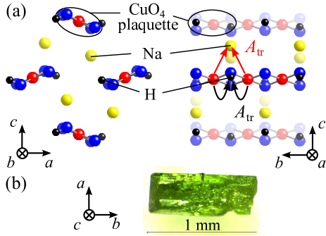
Figure 1: (a) Crystal structure of $\mathrm{NaCuMoO_{4}(OH)}$ along $b$- and $a$-axes. Red, yellow, black, and blues spheres represent Cu, Na, H, and O atoms, respectively, while Mo and a part of O atoms are omitted for clarity. Arrows schematically describe transferred hyperfine interactions of Na and H nuclei with their two nearest Cu sites. (b) Photograph of the single-crystalline $\mathrm{NaCuMoO_{4}(OH)}$ used for heat-capacity and NMR measurements.

.

III Results and Discussions

III.1 Estimation of coupling tensors

First, we discuss hyperfine coupling tensors $\mathbf{A}$ for both ²³Na and ¹H nuclei, which are necessary to determine magnetic structures from NMR spectra (see Section III.3) and spin fluctuations from $1/T_{1}$ quantitatively (see Section III.4). The positions of Na and H atoms in $\mathrm{NaCuMoO_{4}(OH)}$ are illustrated in Fig. 1(a). Na atoms are located in the middle of two Cu chains consisting of edge-sharing $\mathrm{CuO_{4}}$ plaquettes, and H atoms are bonded to O atoms on $\mathrm{CuO_{4}}$ plaquettes. All Na or H atoms are crystallographically equivalent and occupy $4c$ sites. They are also symmetrically equivalent for $B\parallel ab$ and $B\parallel bc$ while they can split into two inequivalent sites when the magnetic field is applied along the other directions. The atomic coordinates of Na and H atoms are (0.3697(5), 1/4, 0.3056(4))NaCuMoO4OH2 and (0.243(4), 1/4, 0.030(4))NaCuMoO4OH4 , respectively. The atomic position of H atoms was determined from neutron diffraction experimentsNaCuMoO4OH4 , and it was also confirmed by density functional theory (DFT) calculations with the generalized gradient approximation plus onsite repulsion $U$, which yield (0.25015, 1/4, 0.01952). The detailed procedure of DFT calculations is the same as described in Ref. DFT, .

The internal field $\mathbf{B}_{\mathrm{int}}$ at a ligand nucleus is expressed by $\mathbf{B}_{\mathrm{int}}=\sum_{i}\mathbf{A}^{i}\cdot\mathbf{\mu}^{i}$, where $\mathbf{A}^{i}$ is the hyperfine coupling tensor and $\mathbf{\mu}^{i}$ is the magnetic moment of the $i$-th Cu site. $\sum_{i}\mathbf{A}^{i}$ appears in a linear relation between the magnetic shift $\mathbf{K}$ and magnetic susceptibility $\chi$ in the paramagnetic phase:

$$\mathbf{K}=\frac{1}{N\mu_{B}}\sum_{i}\mathbf{A}^{i}\cdot\mathbf{\chi}.$$ (1)

We first determined $\sum_{i}\mathbf{A}^{i}$ from Eq. (1) experimentally and then estimated each $\mathbf{A}^{i}$.

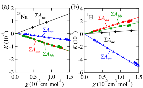
Figure 2: $K$–$\chi$ plots for (a) ²³Na and (b) ¹H nuclei. Lines indicate linear fits to estimate coupling tensors, which are listed in Table 1.

The linear relation (1) for the diagonal components $K_{\epsilon\epsilon}(\epsilon=a,b,c)$ are confirmed by the $K$–$\chi$ plots shown in Fig. 2. They are defined by the observed resonance frequency

$$\nu_{\mathrm{res}}^{(\epsilon)}=(1+K_{\epsilon\epsilon})\gamma B,$$ (2)

and $\sum_{i}A_{\epsilon\epsilon}^{i}$ is determined from the linear slope of the $K_{\epsilon\epsilon}$–$\chi$ plot. The values of $\sum_{i}A_{\epsilon\epsilon}^{i}$ determined experimentally are listed as $\sum_{i}\mathbf{A}_{\mathrm{exp}}^{i}$ in Table. 1.

The nondiagonal components also follow the linear relation (1). While $K_{ab}$ and $K_{bc}$ become 0 because of symmetry and, thus, $A_{ab}$ and $A_{bc}$ cannot be determined, $K_{ac}$ can be determined by the angle dependences of the resonance frequency $\mathbf{\nu}_{\mathrm{res}}$. For $B\parallel ac$, the crystallographically equivalent sites can split into two inequivalent sites for either ²³Na or ¹H. In fact, two resonance lines are observed in the ¹H NMR spectra. Their angle dependences $\mathbf{\nu}(\theta)_{\mathrm{res}}$ are fitted to the following function:

$$\begin{split}\nu(\theta)_{\mathrm{res}}&=(1+K_{aa}\cos^{2}\theta\pm 2K_{ac}\sin\theta\cos\theta\\ &+K_{cc}\sin^{2}\theta)\gamma B,\end{split}$$ (3)

with $K_{aa}$ and $K_{cc}$ fixed to the values determined from Eq. (2). This fit reproduces $\mathbf{\nu}(\theta)_{\mathrm{res}}$ well, as shown in Fig. 3(b), and yields $K_{ac}=3.51\times 10^{-3}$ by using $K_{aa}=1.37\times 10^{-3}$ and $K_{cc}=-3.19\times 10^{-3}$ at 50 K.

For ²³Na nuclei, the quadrupole interaction produces three peaks per site. Thus, six resonance lines are observed in ²³Na spectra. The angle dependence of their positions are fit to the functions including the contributions of the magnetic shift and quadrupole splitting angle :

$$\nu^{I}_{m,m-1}(\theta)_{\mathrm{res}}=(1+K_{aa}\cos^{2}\theta\pm 2K_{ac}\sin\theta\cos\theta$$

$$+K_{cc}\sin^{2}\theta)\gamma B$$

$$-\frac{1}{2}\left(m-\frac{1}{2}\right)\nu_{Q}+\frac{1}{2}\left(m-\frac{1}{2}\right)\nu_{Q}\eta\cos 2(\theta-\theta_{Q})$$

$$-\frac{\nu_{Q}^{2}}{32\gamma B}\{6m(m-1)-2I(I+1)+3\}$$

$$\ \ \ \times\left(1+\frac{2}{3}\eta\cos 2(\theta\mp\theta_{Q})\right)$$ (4)

$$+\frac{\nu_{Q}^{2}\eta^{2}}{72\gamma B}\Bigg{[}24m(m-1)-4I(I+1)+9$$

$$-\left\{\frac{51}{2}m(m-1)-\frac{9}{2}I(I+1)+\frac{39}{4}\right\}$$

$$\ \ \ \times\cos^{2}2(\theta\mp\theta_{Q})\Bigg{]}.$$

$I$ and $m$ are constants that represent a nuclear spin of 3/2 and its $z$-component (3/2, 1/2, or -1/2), respectively. $\nu_{Q}$ is a quadruplole frequency along the maximam principal axis, $\eta$ is an asymmetry parameter, and $\theta_{Q}$ is the angle between the $a$-axis and the closest principal axis of the electric-field gradient; note that the principal axes of the electric-field gradient exist in the $ac$-plane and along the $b$-axis. The free parameters in this fit are $\eta$, $\theta_{Q}$, and $K_{ac}$. $\nu_{Q}$ is determined from NMR spectra for $B~{}\parallel~{}b$, and $K_{aa}$ and $K_{cc}$ are fixed at the values determined from Eq. (2). The fit at 50 K, which is shown in Fig. 3(a), reproduces $\mathbf{\nu}(\theta)_{\mathrm{res}}$ well and yields $\eta$ = 0.532, $\theta_{Q}$ = 18.1^∘, and $K_{ac}=8.85\times 10^{-4}$ by using $\nu_{Q}$ = 1.074 MHz, $K_{aa}=-6.98\times 10^{-4}$, and $K_{cc}=-3.24\times 10^{-4}$. We determined $\sum_{i}A_{ac}^{i}$ from the linear slope of the $K_{ac}$–$\chi$ plot, as shown in Fig. 2. Their values are listed in Table 1.

Table 1: Coupling tensors for ²³Na and ¹H nuclei. $\sum_{i}\mathbf{A}^{i}_{\mathrm{exp}}$, $\sum_{i}\mathbf{A}^{i}_{\mathrm{dip}}$, and $\sum_{i}\mathbf{A}^{i}_{\mathrm{tr}}$ describe the total, dipolar, and transferred hyperfine contributions, respectively. $\sum_{i}\mathbf{A}^{i}_{\mathrm{dip}}$ includes the sum of the Lorentz and demagnetization field, which is estimated as $-$0.010 ($aa$), 0.020 ($bb$), $-$0.010 T/$\mu_{\mathrm{B}}$ ($cc$) demag . The values of the transferred hyperfine coupling adopted for the simulation are listed as $\sum_{i}\mathbf{A}^{i}_{\mathrm{tr,sim}}$. All values are described in units of T/$\mu_{\mathrm{B}}$.

		$\sum_{i}\mathbf{A}^{i}_{\mathrm{exp}}$	$\sum_{i}\mathbf{A}^{i}_{\mathrm{dip}}$	$\sum_{i}\mathbf{A}^{i}_{\mathrm{tr}}$	$\sum_{i}\mathbf{A}^{i}_{\mathrm{tr,sim}}$
	$aa$	$-$0.054(10)	$-$0.015(10)	$-$0.039(14)	$-$0.050
23Na	$bb$	$-$0.052(10)	$-$0.009(10)	$-$0.043(14)	$-$0.043
	$cc$	$-$0.022(10)	0.024(10)	$-$0.046(14)	$-$0.038
	$ac$	0.059(10)	0.066(10)	$-$0.007(14)	0
	$aa$	0.099(10)	0.085(10)	0.014(14)	0.014
1H	$bb$	0.066(10)	0.031(10)	0.035(14)	0.035
	$cc$	$-$0.193(10)	$-$0.115(10)	$-$0.078(14)	$-$0.078
	$ac$	0.021(10)	0.036(10)	$-$0.015(14)	$-$0.010

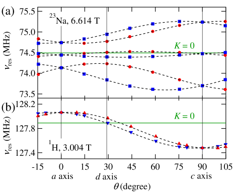
Figure 3: Angle dependences of resonance frequencies for (a) ²³Na and (b) ¹H nuclei at 50 K. Two inequivalent sites are colored in red and blue. Dashed curves represent the fitting curves of Eq. (3) for ¹H and those of Eq. (4) for ²³Na. Horizontal lines represent frequencies corresponding to $K=0$. The $d$-axis is the specific axis defined in the main text.

Next, we estimated $\mathbf{A}^{i}$ from the coupling tensor determined experimentally, $\sum_{i}\mathbf{A}_{\mathrm{exp}}^{i}$, in the following manner. $\sum_{i}\mathbf{A}_{\mathrm{exp}}^{i}$ can be divided into two contributions: $\sum_{i}\mathbf{A}_{\mathrm{dip}}^{i}$ and $\sum_{i}\mathbf{A}_{\mathrm{tr}}^{i}$. $\sum_{i}\mathbf{A}_{\mathrm{dip}}^{i}$ is calculated by a lattice sum of dipolar interactions within a sphere with a radius of 60 Å  together with a Lorentz field and a demagnetization field. The sum of the Lorentz and demagnetization field is estimated as $-$0.010, 0.020, $-$0.010 T/$\mu_{\mathrm{B}}$ for the $a$-, $b$-, $c$-components, respectively, from the crystal shapedemag . The contribution of transferred hyperfine interactions corresponds to the difference, $\sum_{i}\mathbf{A}_{\mathrm{tr}}^{i}\equiv\sum_{i}\mathbf{A}_{\mathrm{exp}}^{i}-\sum_{i}\mathbf{A}_{\mathrm{dip}}^{i}$. We assumed that $\sum_{i}\mathbf{A}^{i}_{\mathrm{tr}}$ consists of contributions from only two nearest-neighbor Cu sites as schematically illustrated by the red arrows in Fig. 1(a), since transferred hyperfine interactions are short-ranged. This assumption is applicable for ¹H nuclei since the distance from a H atom to the nearest Cu atom is 2.500 Å, while that to the next-nearest Cu atom is 4.905 Å. For ²³Na nuclei, the distance between Na and O is important since the transferred hyperfine interactions are mediated by Cu-O-Na paths. The distance for the shortest path is 2.321 Å and is considerably smaller than that for the next-shortest path of 2.806 Å. Thus, the assumption would be reasonable for ²³Na nuclei as well.

The transferred hyperfine coupling used to analyze NMR spectra and $1/T_{1}$ is listed in Table 1 as $\sum_{i}\mathbf{A}^{i}_{\mathrm{tr,sim}}$. While the transferred contribution for ²³Na nuclei is almost isotropic, that for ¹H nuclei is anistropic. This anisotropy might be caused by the distribution of the magnetic moments over ligand O atoms due to the covalent bonding between Cu 3d and O 2s/2p orbitals, which modifies the dipolar contribution. Indeed, in several other compounds, the calculation of a hyperfine coupling constant is improved by putting a fraction of the magnetic moments on the ligand O atomsPbCuSO4OH_7 ; hyperfine ; hyperfine2 . However, in this compound, the remaining anistropy of hyperfine coupling cannot be reproduced by the same method. Thus, we adopt the values determined under the assumption that the moments are only on Cu sites.

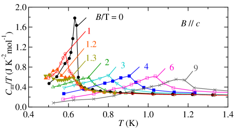
Figure 4: Temperature dependences of $C_{m}/T$ for $B~{}\parallel~{}c$.

III.2 Phase diagram

Before discussing magnetic structures and spin fluctuations, let us start with variations of the magnetic heat capacity $C_{m}$ and ²³Na NMR spectra in order to establish a magnetic phase diagram. The temperature dependence of $C_{m}/T$ at $B~{}\parallel~{}c$ is shown in Fig. 4. A sharp peak is observed at 0.63(1) K in zero field, indicating a magnetic phase transitionNaCuMoO4OH . With an increasing magnetic field, the peak shifts to lower temperatures and splits into two peaks above 1 T. The low-$T$ peak continues to move to lower temperatures and disappears below 0.5 K above 2 T, whereas the high-$T$ peak shifts to higher temperatures and finally reaches 1.16 K at 9 T. These field dependences suggest the presence of two phases at low fields, which is confirmed by ²³Na NMR measurements.

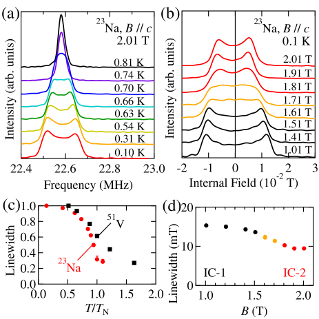
Figure 5: (a) Temperature evolution of ²³Na NMR spectra (center line) at $B$ = 2.01 T and $B~{}\parallel~{}c$. (b) Variation of ²³Na NMR spectra (center line) as a function of a magnetic field at $T$ = 0.1 K and $B~{}\parallel~{}c$. (c) Normalized linewidth of the ²³Na NMR spectra shown in Fig. 5(a) as a function of temperature, which is estimated from a second moment (red circles). It is compared with the linewidth of ⁵¹V NMR spectra measured at $B$ = 10 T and $B~{}\parallel~{}c$ for $\mathrm{LiCuVO_{4}}$ (black squares) NMR6 . (d) Field dependence of a linewidth estimated from ²³Na NMR spectra shown in Fig. 5(b). The linewidths in Fig. (c, d) are determined by calculating second moments.

Figure 5(a) shows the temperature dependence of ²³Na NMR spectra at 2 T. A sharp peak observed at 0.8 K and 2 T clearly becomes broad at lower temperatures. The temperature dependence of the linewidth is shown in Fig. 5(c). $T_{\mathrm{N}}=$ 0.7 K, determined by the onset temperature for line broadening, coincides with the peak temperature at 2 T in $C_{m}/T$. The spectrum at 0.1 K shows a double-horn type lineshape, which is characteristic of an incommensurate spiral or SDW order. Figure 5(b) shows a field evolution of NMR spectra. A double-horn-type lineshape is also observed under lower magnetic fields. Their linewidths are plotted as a function of a magnetic field in Fig 5(d). A clear change in the linewidth is detected across $B_{c}$ = 1.51–1.81 T, indicating a field-induced magnetic phase transition between two incommensurate phases; we name the two phases below and above $B_{c}$ as IC-1 and IC-2, respectively. The transition between the two phases is observed at $B_{c}$ = 1.81–2.01 T for $B\parallel a$. The difference in $B_{c}$ can be explained by the anisotropy of the $g$-factorNaCuMoO4OH3 .

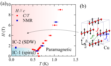
Figure 6: (a) Magnetic phase diagram of $\mathrm{NaCuMoO_{4}(OH)}$ for $B~{}\parallel~{}c$. Two sets of $T_{\mathrm{N}}$ from heat capacity and ²³Na NMR measurements are plotted. (b) Schematic view of the magnetic structure in the IC-2 phase and dominant interactions.

All $T_{\mathrm{N}}$ from the heat-capacity and NMR measurements are plotted in the $B$-$T$ phase diagram of Fig. 6(a). IC-1 is quickly suppressed by $B$, while IC-2 becomes stable above $B_{c}$ with its $T_{\mathrm{N}}$ increasing with an increasing magnetic field. Provided that the present compound is best described as a $J_{1}$–$J_{2}$ chain magnet, IC-1 and IC-2 would correspond to spiral and SDW phases, respectively 1Dtheory2 ; 1Dtheory3 . DMRG calculations of a $J_{1}$–$J_{2}$ chain model show that the corresponding critical field is 0.05 $J_{2}$ for $J_{1}/J_{2}$ = $-$51/36 1Dtheory2 ; 1Dtheory3 , which corresponds to 1.2 T, reasonably close to the observed $B_{c}$.

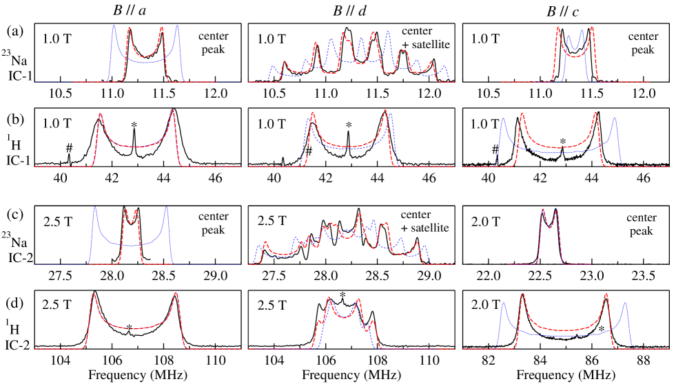
Figure 7: ²³Na and ¹H NMR spectra for IC-1 (a, b) and IC-2 (c, d) measured at 0.1 K. The left, middle, and right panels show the NMR spectra for $B~{}\parallel~{}a$, $B~{}\parallel~{}d$, and $B~{}\parallel~{}c$, respectively, where the $d$ direction is canted from the $c$-axis to the $a$-axis by 61^∘ (see Fig. 3). The left and right panels of (a) and (c) show only center peaks of the ²³Na NMR signals since satellite peaks exhibit the same lineshape as the center one. For the middle panels, two satellite peaks are also included since they cannot be separated from the center line. An analytic deconvolution is applied to the quadrupole splitting of the NMR spectra in the top panel of (a) deconvolution . In each panel, the experimental NMR spectrum (black solid curves) is compared with simulated spectra for the spiral (IC-1) or SDW (IC-2) order with the ferromagnetic (red dashed curves) and antiferromagnetic (blue dotted curves) interchain coupling $J^{\prime}$. Symbols * and # represent extrinsic signals from ¹H and ¹⁹F nuclei, respectively.

III.3 Magnetic structures at ordered phases

To determine the magnetic structures of IC-1 and IC-2, we carefully performed ²³Na and ¹H NMR measurements with the three orientations of $B~{}\parallel~{}a$, $B~{}\parallel~{}d$, and $B~{}\parallel~{}c$, where the $d$ direction is canted from the $c$ axis to $a$ axis by 61^∘. The $d$ direction is selected so that one set of a magnetic shift for ¹H nuclei becomes almost 0, as shown in Fig. 3(b). The obtained spectra are shown by the black solid curves in Fig. 7. For $B~{}\parallel~{}a$ and $c$ (the left and right panels), there is a unique site either for a Na or H atom in the paramagnetic state so that an incommensurate magnetic order produces a single resonance line with a double-horn structure. On the other hand, the NMR spectra for $B~{}\parallel~{}d$ (the middle panels) can be complex because two inequivalent sites are present either for a Na or H atom, unless for $B\parallel ab$ or $bc$, which lead to the overlap of the two double-horn lineshapes. Such a complex $B~{}\parallel~{}d$ spectrum could be decisive in determining the spin structure. Note that a ²³Na NMR spectrum also contains two satellite peaks together with the center peak, thus totally a superposition of six double-horn lineshapes appears.

First, we discuss the ¹H NMR spectra in IC-1 (Fig. 7(b)) and IC-2 (Fig. 7(d)). While the ¹H NMR spectra in IC-1 are insensitive to the applied field direction, the spectral width in IC-2 is strongly dependent on the field direction. This field-direction dependence in IC-2 agrees well with the angular dependence of the paramagnetic shift shown in Fig. 3(b), indicating that the ordered moments in IC-2 are parallel to the field direction. Thus, the magnetic structure in IC-2 is considered to be SDW, as expected in the $J_{1}$–$J_{2}$ chain. On the other hand, it is difficult to deduce the magnetic structure for IC-1, where a spiral order is expected. This is because the transverse ordered moments combined with the off-diagonal component of the hyperfine coupling can also contribute to the internal field, and thus, the angular dependence of the NMR spectra for a spiral order is not straightforward.

To examine details of the magnetic structures, we performed a simulation of the spectra by constructing a histogram of the resonance frequency $\nu$ = $\gamma|\mathbf{B}+\mathbf{B}_{\mathrm{int}}|$ and then convoluting it with a Gaussian function. To obtain the distribution of $\nu$, the internal field $\mathbf{B}_{\mathrm{int}}$ is calculated as $\mathbf{B}_{\mathrm{int}}$ = $\sum_{i}\mathbf{A}^{i}\cdot\mathbf{\mu}^{i}$, where $\mathbf{A}^{i}$ is the hyperfine coupling tensor discussed in Section III.1 and $\mathbf{\mu}^{i}$ is the magnetic moment of an assumed spin structure at the i-th Cu site within a distance of 60 Å from the nuclei. Note that the $ab$- and $bc$-components of the transferred hyperfine coupling, which cannot be determined in the paramagnetic phase, are set to zero. These components have almost no influence on our final result, since there is no ordered moment along the $b$-axis. The NMR spectra could not be reproduced by spiral structures in the $ab$- or $bc$-plane even if $A_{ab}$ and $A_{bc}$ are treated as adjustable parameters.

For IC-2, the magnetic structure is expected to be an SDW order structure with spins aligned parallel to the magnetic field and modulated sinusoidally along the spin chain. We have performed simulations for two cases: the case of ferromagnetic interchain coupling (defined as $J^{\prime}$ in Fig. 6(b)) and of antiferromagnetic interchain coupling. The magnetic wave vectors of the two cases are $\mathbf{Q}=2\pi(0,\alpha,0)$ and $2\pi(1,\alpha,0)$, respectively, where $\alpha$ is $\alpha=1/2-M/(g\mu_{B})$ ($M$ is the magnetization) deduced from the $J_{1}$–$J_{2}$ chain model 1Dtheory2 ; 1Dtheory3 ; 1DtheoryofT11 ; note that the unit cell includes two Cu sites in a single chain. As shown in Figs. 7(c, d), the simulation for ferromagnetic $J^{\prime}$ (red dashed curves) can reproduce all of the experimental spectra, whereas that for antiferromagnetic $J^{\prime}$ (blue dotted curves) cannot. Thus, the SDW with ferromagnetic $J^{\prime}$, as shown in Fig. 6(b), is the most likely candidate. Note that the amplitude of the SDW is the only free parameter except for $\mathbf{A}_{\mathrm{tr}}$, which has little uncertainty. The amplitude is estimated to be 0.38 $\mu_{\mathrm{B}}$, assuming that it is independent of the field orientation. It is smaller than the value of 0.6–0.8 $\mu_{\mathrm{B}}$ for $\mathrm{LiCuVO_{4}}$ NMR4 , which may be due to larger quantum fluctuations associated with better one dimensionality in $\mathrm{NaCuMoO_{4}(OH)}$.

On the other hand, we have examined four likely cases for IC-1: the spiral plane always perpendicular to the field direction or parallel to the $ab$-, $bc$-, or $ac$-plane regardless of the field direction. The magnetic wave vector is $\mathbf{Q}=2\pi(0,\beta,0)$, where $\beta$ is $\beta=\arccos(-J_{1}/4J_{2})/\pi$ in a classical $J_{1}$–$J_{2}$ chain. Among the four cases, all of the experimental spectra are well reproduced only when the spiral plane is parallel to the $ac$-plane, as shown in Figs. 7(a, b). Only the $ac$-spiral order with ferromagnetic $J^{\prime}$ is consistent with the experimental spectra. The magnitude of the ordered moments is estimated to be 0.29 $\mu_{\mathrm{B}}$. Note that this value, based on the classical model, may be an underestimation since quantum effects should lead to a larger pitch angle of the spiral, resulting in narrower NMR spectra. In brief summary, the NMR spectra indicate the spiral and SDW orders in IC-1 and IC-2, respectively, as expected from the frustrated $J_{1}$–$J_{2}$ chain model.

III.4 Anisotropic spin fluctuations

Another evidence for the $J_{1}$–$J_{2}$ chain magnet is found in the presence of anisotropic spin fluctuations due to the formation of magnon bound states. Figures 8(a) and 8(b) show the temperature dependences of $1/T_{1}$ at $B\parallel c$ for ²³Na ($1/^{23}T_{1}$) and ¹H ($1/^{1}T_{1}$), respectively. $1/^{23}T_{1}$ behaves similarly below and above $B_{c}$; it increases with decreasing temperature and exhibits a peak at $T_{\mathrm{N}}$ owing to the critical slowing down of spin fluctuations. In sharp contrast, $1/^{1}T_{1}$ changes its temperature dependence remarkably across $B_{c}$: the enhancement in $1/^{1}T_{1}$ observed at 1.01 T near $T_{\mathrm{N}}$ is suppressed at 2.01 T just above $B_{c}$. At higher magnetic fields, $1/^{1}T_{1}$ decreases with decreasing temperature and follows an activation-type temperature dependence above $T_{\mathrm{N}}$. This is confirmed by an Arrhenius plot of $1/^{1}T_{1}$ in Fig. 9(a). At 10 T, the activation energy is estimated to be $\Delta$ = 2.9(1) K $\sim$ 0.08 $J_{2}$.

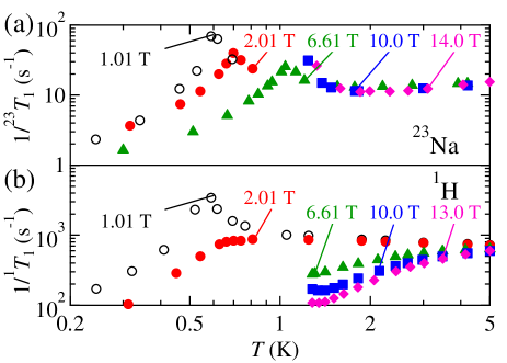
Figure 8: Temperature dependences of $1/T_{1}$ at $B\parallel c$ for (a) ²³Na and (b) ¹H nuclei.

In order to understand the difference between the temperature dependences of $1/^{23}T_{1}$ and $1/^{1}T_{1}$, it is necessary to investigate the form factor for both nuclei. In general, $(1/T_{1})_{\xi}$, where $\xi$ denotes the field direction, is given by the sum of both transverse and longitudinal spin correlation functions $S_{\perp}(\mathbf{q},\omega)$ and $S_{\parallel}(\mathbf{q},\omega)$NMR2 :

$$\begin{split}\left(\frac{1}{T_{1}}\right)_{\xi}&=\frac{1}{N}\sum_{\mathbf{q}}\{\Gamma^{\perp}_{\xi}(\mathbf{q})S_{\perp}(\mathbf{q},\omega)+\Gamma^{\parallel}_{\xi}(\mathbf{q})S_{\parallel}(\mathbf{q},\omega)\},\end{split}$$ (5)

where $N$ is the number of atoms, and $\Gamma^{\perp}_{\xi}(\mathbf{q})$ and $\Gamma^{\parallel}_{\xi}(\mathbf{q})$ are form factors defined as in Ref. NMR2, . For $B\parallel c$, they become

$$\begin{split}\Gamma^{\perp}_{c}(\mathbf{q})&=\frac{\gamma^{2}}{2}\{g_{aa}^{2}|A(\mathbf{q})_{aa}|^{2}+g_{bb}^{2}|A(\mathbf{q})_{bb}|^{2}\\ &\ \ \ \ +(g_{aa}^{2}+g_{bb}^{2})|A(\mathbf{q})_{ab}|^{2}\}\\ \Gamma^{\parallel}_{c}(\mathbf{q})&=\frac{\gamma^{2}}{2}g_{cc}^{2}\left(|A(\mathbf{q})_{ac}|^{2}+|A(\mathbf{q})_{bc}|^{2}\right),\end{split}$$ (6)

where $A(\mathbf{q})_{\mu\nu}$ is a Fourier sum of hyperfine coupling constants, $A(\mathbf{q})_{\mu\nu}=\sum_{i}A^{i}_{\mu\nu}e^{i\mathbf{q}\cdot\mathbf{r}}$, taken over all Cu sites within a distance of 60 Å from the nuclei. In a small temperature range just above $T_{\mathrm{N}}$, where spin fluctuations are dominated by the component with the $\mathbf{q}$-vector in the ordered phase $\mathbf{Q}_{0}$, the $q$-dependent hyperfine coupling constants in Eq. (5) can be approximately replaced by their values at $\mathbf{Q}_{0}$NMR2 :

$$\left(\frac{1}{T_{1}}\right)_{\xi}\simeq\Gamma^{\perp}_{\xi}(\mathbf{Q}_{0})\langle S_{\perp}(\mathbf{q},\omega)\rangle+\Gamma^{\parallel}_{\xi}(\mathbf{Q}_{0})\langle S_{\parallel}(\mathbf{q},\omega)\rangle,$$ (7)

where $\langle S_{\perp}(\mathbf{q},\omega)\rangle$ and $\langle S_{\parallel}(\mathbf{q},\omega)\rangle$ represent q-averages of the transverse and longitudinal spin correlation functions, respectively.

Equation (7) indicates that $\langle S_{\perp}(\mathbf{q},\omega)\rangle$ and $\langle S_{\parallel}(\mathbf{q},\omega)\rangle$ close to $T_{N}$ can be extracted by calculating $\Gamma^{\perp}_{c}\equiv\Gamma^{\perp}_{\xi}(\mathbf{Q}_{0})$ and $\Gamma^{\parallel}_{c}\equiv\Gamma^{\parallel}_{\xi}(\mathbf{Q}_{0})$ from the hyperfine coupling tensor and the magnetic wave vector $\mathbf{Q}_{0}$ = $2\pi(0,\alpha,0)$. We adopt the transferred hyperfine coupling constants listed in Table 1 for this calculation. The $ab$- and $bc$-components of the transferred hyperfine coupling tensor, which cannot be determined experimentally, are assumed to be zero. For ²³Na nuclei, $\Gamma^{\perp}_{c}$ and $\Gamma^{\parallel}_{c}$ are estimated as 7.5 $\times$ 10¹³ and 3.8 $\times$ 10¹³ s^-2 at 2 T, respectively, leading to $\Gamma^{\perp}_{c}/\Gamma^{\parallel}_{c}$ = 2.0. Thus, both the transverse and longitudinal spin fluctuations affect $1/^{23}T_{1}$. On the other hand, the same procedure provides a $\Gamma^{\perp}_{c}$ much larger than $\Gamma^{\parallel}_{c}$ for ¹H nuclei: 6.2 $\times$ 10¹⁵ and 1.0 $\times$ 10¹⁴ s^-2, respectively ($\Gamma^{\perp}_{c}/\Gamma^{\parallel}_{c}$ = 60). This is because H and Cu atoms are almost in the same $c$-plane, and thus, dominant dipole-dipole interactions provide $|A_{ac}|$ and $|A_{bc}|$ much smaller than $|A_{aa}|$ and $|A_{ab}|$. The large $\Gamma^{\perp}_{c}/\Gamma^{\parallel}_{c}$ indicates that $1/^{1}T_{1}$ is only sensitive to transverse fluctuations. Based on both form factors, we come to the following conclusion: the activated temperature dependence in $1/^{1}T_{1}$ reveals the presence of gapped transverse excitations, while the strong increase near $T_{\mathrm{N}}$ in $1/^{23}T_{1}$ indicates gapless longitudinal excitations. In addition, the above conclusion is not changed by the uncertainty of $A_{ab}$ and $A_{bc}$. Even if an additional contribution of $A_{\mathrm{tr}}$ comparable with $A_{\mathrm{dip}}$ is added in the Fourier sum, $\Gamma_{c}^{\perp}/\Gamma_{c}^{\parallel}\sim 1$ for ²³Na and $\Gamma_{c}^{\perp}/\Gamma_{c}^{\parallel}\gg 1$ for ¹H are still satisfied.

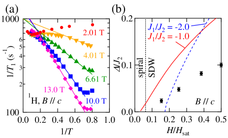
Figure 9: (a) Arrhenius plot of $1/^{1}T_{1}$ measured at 2–13 T. (b) Field dependence of the excitation gap determined from $1/^{1}T_{1}$. Red solid and blue dashed curves represent field dependences of magnon binding energy in a frustrated $J_{1}$-$J_{2}$ chain with $J_{2}/J_{1}$ = $-$1.0 and $-$2.0 calculated from DMRG calculations1Dtheory5 .

Such anisotropic spin fluctuations are consistent with the formation of bound magnons expected in the $J_{1}$–$J_{2}$ chain magnet. The gap cannot be explained by the Zeeman energy, since it induces a gap in a longitudinal spectrum, which is inconsistent with the anisotropic gap in this compound. The gap corresponds to the magnon binding energy, which is the energy cost to separate a magnon bound pair into two single magnons, resulting in gapped transverse excitations 1DtheoryofT11 ; 1DtheoryofT12 . At the same time, longitudinal fluctuations are developed because of density fluctuations of bound magnons. The field dependence of the gap estimated from the Arrhenius plot is compared with the magnon binding energy in a frustrated $J_{1}$-$J_{2}$ chain determined from DMRG calculations in Fig. 9(b)1Dtheory5 . The gap becomes large with increasing field, which is qualitatively consistent with the field dependence of the magnon binding energy. However, its magnitude is almost half of that of the $J_{1}$-$J_{2}$ chain model. This may be due to Dzyaloshinskii-Moriya interactions not included in the DMRG calculation, which can be the same magnitude as the magnon binding energy. Note that Dzyaloshinskii-Moriya interactions between nearest neighbors are present while those between next-nearest neighbors are absent because of inversion symmetry at each Cu site.

IV Comparison with other candidates

The present study reveals that $\mathrm{NaCuMoO_{4}(OH)}$ realizes a $J_{1}$–$J_{2}$ chain magnet from both macroscopic and microscopic probes. Compared with other candidates, the magnetic properties of $\mathrm{NaCuMoO_{4}(OH)}$ are quite similar to those of $\mathrm{LiCuVO_{4}}$. For instance, the phase diagram of these materials has the same character at low fields: the spiral and collinear SDW phases are present, and the transition temperature of the spiral phase decreases but that of the collinear SDW phase increases with an increasing fieldPD_LCVO ; NMR4 ; HFHC . Additional intermediate phases triggered by competition among interchain interactions, such as a complex collinear SDW phase in $\mathrm{PbCu(SO_{4})(OH)_{2}}$PbCuSO4OH_3 ; PbCuSO4OH_6 ; PbCuSO4OH_8 and a spin-stripe phase in $\mathrm{TeVO_{4}}$TeVO4_3 ; TeVO4_4 , have not been detected so far. The difference indicates that interchain interactions are weak in $\mathrm{NaCuMoO_{4}(OH)}$.

The difference between $\mathrm{NaCuMoO_{4}(OH)}$ and $\mathrm{LiCuVO_{4}}$ is that the former compound has a great advantage to obtain high-quality single crystals with less disorder as well as $\mathrm{PbCu(SO_{4})(OH)_{2}}$PbCuSO4OH_0 ; PbCuSO4OH_2 ; PbCuSO4OH_3 ; PbCuSO4OH_4 ; PbCuSO4OH_6 ; PbCuSO4OH_7 ; PbCuSO4OH_8 ; PbCuSO4OH_9 , 3-I-V3IV , and $\mathrm{TeVO_{4}}$TeVO4 ; TeVO4_2 ; TeVO4_3 ; TeVO4_4 , while the latter compound has difficulties in avoiding disorder effects. $C_{m}/T$ and the linewidth of NMR spectra in the vicinity of $T_{\mathrm{N}}$ can be indicators of the degree of disorder. $C_{m}/T$ exhibits a sharp peak at $T_{\mathrm{N}}$ in $\mathrm{NaCuMoO_{4}(OH)}$ (Fig. 4), in contrast to the much broader peak in $\mathrm{LiCuVO_{4}}$neutron2 ; HFHC . Moreover, the second moment of NMR spectra exhibits an abrupt change in $\mathrm{NaCuMoO_{4}(OH)}$ below $T_{\mathrm{N}}$, while it exhibits a broad variation in the ⁵¹V NMR spectra of $\mathrm{LiCuVO_{4}}$ NMR6 , as compared in Fig. 5(c). The availability of high-quality crystals is important since the nematic state might be significantly suppressed by disorder, especially in high fields, and the transition should be sharp to detect the nematic state expected in the very narrow field range. In addition, the smaller saturation field of $\mathrm{NaCuMoO_{4}(OH)}$ compared to that of $\mathrm{LiCuVO_{4}}$ makes high-field experiments easier. From these viewpoints, $\mathrm{NaCuMoO_{4}(OH)}$ is a promising compound to investigate unique field-induced phases in the $J_{1}$–$J_{2}$ chain magnet.

V Summary

In summary, we performed heat-capacity and NMR measurements on a single crystal of $\mathrm{NaCuMoO_{4}(OH)}$. A magnetic-field-induced transition is found at $B_{c}$ $\sim$ 1.8 T from an incommensurate spiral order to an incommensurate longitudinal SDW order in which anisotropic spin fluctuations indicating the formation of bound magnons are observed by $1/T_{1}$ measurements. Therefore, $\mathrm{NaCuMoO_{4}(OH)}$ is a good candidate frustrated $J_{1}$–$J_{2}$ chain magnet and would provide us an opportunity to investigate the hidden spin nematic order and fluctuations near the magnetic saturation through further high-field NMR and neutron scattering experiments.

- (1) H.-J. Mikeska and A. K. Kolezhuk, in Quantum Magnetism, edited by U. Schollwöck et al., Lecture Notes in Physics Vol. 645 (Springer-Verlag, Berlin, 2004), p. 1.
- (2) G. Misguich and C. Lhuillier, in Frustrated Spin Systems, edited by H. T. Diep (World Scientific, Singapore, 2005), p. 229.
- (3) L. Balents, Nature 464, 199 (2010).
- (4) M. E. Zhitomirsky and K. Ueda, Phys. Rev. B 54, 9007 (1996).
- (5) F. Andreev and I. A. Grishchuk, Zh. Eksp. Teor. Fiz. 87, 467 (1984).
- (6) N. Shannon, T. Momoi, and P. Sindzingre, Phys. Rev. Lett. 96, 027213 (2006).
- (7) H. T. Ueda and T. Momoi, Phys. Rev. B 87, 144417 (2013).
- (8) A. V. Chubukov, Phys. Rev. B 44, 4693 (1991).
- (9) L. Kecke, T. Momoi, and A. Furusaki, Phys. Rev. B 76 060407 (2007).
- (10) T. Vekua, A. Honecker, H.-J. Mikeska, and F. Heidrich-Meisner, Phys. Rev. B 76, 174420 (2007).
- (11) T. Hikihara, L Kecke, T. Momoi, and A. Furusaki, Phys. Rev. B 78, 144404 (2008).
- (12) J. Sudan, A. Lûscher, and A. M. Lâuchli, Phys. Rev. B 80, 140402 (2009).
- (13) M. E. Zhitomirsky and H. Tsunetsugu, Europhys. Lett. 92, 37001 (2010).
- (14) M. Sato, T. Hikihara, and T. Momoi, Phys. Rev. Lett. 110, 077206 (2013).
- (15) O. A. Starykh and L. Balents, Phys. Rev. B 89, 104407 (2014).
- (16) L. Balents and O. A. Starykh, Phys. Rev. Lett. 116, 177201 (2016).
- (17) M. A. Lafontaine, M. Leblanc, and G. Ferey, Inorg. Chem. C45, 1205 (1989).
- (18) B. J. Gibson, R. K. Kremer, A. V. Prokofiev, W. Assmus, and G. J. McIntyre, Physica B 350, e253 (2004).
- (19) M. Enderle, C. Mukherjee, B. Fåk, R. K. Kremer, J.-M. Broto, H. Rosner, S.-L. Drechsler, J. Richter, J. Malek, A. Prokofiev, W. Assmus, S. Pujol, J.-L. Raggazzoni, H. Rakoto, M. Rheinstâdter and H. M. Rønnow, Europhys. Lett. 70, 237 (2005).
- (20) N. Büttgen, H. -A. Krug von Nidda, L. E. Svistov, L. A. Prozorova, A. Prokofiev, and W. Aßmus, Phys. Rev. B 76, 014440 (2007).
- (21) M. G. Banks, F. Heidrich-Meisner, A. Honecker, H. Rakoto, J. -M. Broto, and R. K. Kremer, J. Phys.: Condens. Matter, 19 145227 (2007).
- (22) T. Masuda, M. Hagihala, Y. Kondoh, K. Kaneko, and N. Metoki, J. Phys. Soc. Jpn. 80, 113705 (2011).
- (23) M. Mourigal, M. Enderle, B. Fåk, R. K. Kremer, J. M. Law, A. Schneidewind, A. Hiess, and A. Prokofiev, Phys. Rev. Lett. 109, 027203 (2012).
- (24) N. Büttgen, W. Kraetschmer, L. E. Svistov, L. A. Prozorova, and A. Prokofiev, Phys. Rev. B 81, 052403 (2010).
- (25) N. Büttgen, P. Kuhns, A. Prokofiev, A. P. Reyes, and L. E. Svistov, Phys. Rev. B 85, 214421 (2012).
- (26) K. Nawa, M. Takigawa, M. Yoshida, and K. Yoshimura, J. Phys. Soc. Jpn. 82, 094709 (2013).
- (27) K. Nawa, M. Takigawa, S. Krämer, M. Horvatic,́ C. Berthier, M. Yoshida, and K. Yoshimura, Phys. Rev. B 96, 134423 (2017).
- (28) L. E. Svistov, T. Fujita, H. Yamaguchi, S. Kimura, K. Omura, A. Prokofiev, A. I. Smirnov, Z. Honda, and M. Hagiwara, JETP Lett. 93, 21 (2011).
- (29) N. Büttgen, K. Nawa, T. Fujita, M. Hagiwara, P. Kuhns, A. Prokofiev, A. P. Reyes, L. E. Svistov, K. Yoshimura, and M. Takigawa, Phys. Rev. B 90, 134401 (2014).
- (30) L. A. Prozorova, S. S. Sosin, L. E. Svistov, N. Büttgen, J. B. Kemper, A. P. Reyes, S. Riggs, A. Prokofiev, and O. A. Petrenko, Phys. Rev. B 91, 174410 (2015).
- (31) A. Orlova, E. L. Green, J. M. Law, D. I. Gorbunov, G. Chanda, S. Krämer, M. Horvatić, R. K. Kremer, J. Wosnitza, and G. L. J. A. Rikken, Phys. Rev. Lett. 118, 247201 (2017).
- (32) C. Dussarrat, G. C. Mather, V. Caignaert, B. Domenès, J. G. Fletcher, and A. R. West, J. Solid. State Chem. 166, 311 (2002).
- (33) S.-L. Drechsler, O. Volkova, A. N. Vasiliev, N. Tristan, J. Richter, M. Schmitt, H. Rosner, J. Málek, R. Klingeler, A. A. Zvyagin, and B. Buc̈hner, Phys. Rev. Lett. 98, 077202 (2007).
- (34) S. F. Solodovnikov and Z. A. Solodovnikova, Zh. Strukt. Khim. 38 914 (1997)
- (35) M. Hase, H. Kuroe, K. Ozawa, O. Suzuki, H. Kitazawa, G. Kido, and T. Sekine, Phys. Rev. B 70, 104426 (2004).
- (36) H. Effenberger, Mineralogy and Petrology 36, 3 (1987).
- (37) A. U. B. Wolter, F. Lipps, M. Schäpers, S.-L. Drechsler, S. Nishimoto, R. Vogel, V. Kataev, B. Buchner, H. Rosner, M. Schmitt, M. Uhlarz, Y. Skourski, J. Wosnitza, S. Sullow, and K. C. Rule, Phys. Rev. B 85, 014407 (2012).
- (38) B. Willenberg, M. Schäpers, K. C. Rule, S. Süllow, M. Reehuis, H. Ryll, B. Klemke, K. Kiefer, W. Schottenhamel, B. Büchner, B. Ouladdiaf, M. Uhlarz, R. Beyer, J. Wosnitza, and A. U. B. Wolter, Phys. Rev. Lett. 108, 117202 (2012).
- (39) A. U. B. Wolter, F. Lipps, M. Schäpers, S.-L. Drechsler, S. Nishimoto, R. Vogel, V. Kataev, B. Buchner, H. Rosner, M. Schmitt, M. Uhlarz, Y. Skourski, J. Wosnitza, S. Sullow, and K. C. Rule, Phys. Rev. B 85, 014407 (2012).
- (40) M. Schäpers, A. U. B. Wolter, S.-L. Drechsler, S. Nishimoto, K.-H. Müller, M. Abdel-Hafiez, W. Schottenhamel, B. Büchner, J. Richter, B. Ouladdiaf, M. Uhlarz, R. Beyer, Y. Skourski, J. Wosnitza, K. C. Rule, H. Ryll, B. Klemke, K. Kiefer, M. Reehuis, B. Willenberg, and S. Süllow, Phys. Rev. B 88, 184410 (2013).
- (41) M. Schäpers, H. Rosner, S.-L. Drechsler, S. Süllow, R. Vogel, B. Büchner, and A. U. B. Wolter, Phys. Rev. B 90, 224417 (2014).
- (42) B. Willenberg, M. Schäpers, A.U.B. Wolter, S.-L. Drechsler, M. Reehuis, J.-U. Hoffmann, B. Büchner, A.J. Studer, K.C. Rule, B. Ouladdiaf, S. Süllow, and S. Nishimoto, Phys. Rev. Lett. 116, 047202 (2016).
- (43) K. C. Rule, B. Willenberg, M. Schäpers, A. U. B. Wolter, B. Büchner, S.-L. Drechsler, G. Ehlers, D. A. Tennant, R. A. Mole, J. S. Gardner, S. Süllow, and S. Nishimoto, Phys. Rev. B 95, 024430 (2017).
- (44) S. E. Dutton, M. Kumar, M. Mourigal, Z. G. Soos, J.-J. Wen, C. L. Broholm, N. H. Andersen, Q. Huang, M. Zbiri, R. Toft-Petersen, and R. J. Cava, Phys. Rev. Lett. 108, 187206 (2012).
- (45) H. -J. Grafe, S. Nishimoto, M. Iakovleva, E. Vavilova, L. Spillecke, A. Alfonsov, M. -I. Sturza, S. Wurmehl, H. Nojiri, H. Rosner, J. Richter, U. K. R’́oßler, S.-L. Drechsler, V. Kataev and B. Büchner, Sci. Rep. 7, 6720 (2017).
- (46) R. Berger, A. Meetsma, and S. van Smaalen, J. Less-Comm. Met. 175, 119 (1991).
- (47) T. Masuda, A. Zheludev, B. Roessli, A. Bush, M. Markina, and A. Vasiliev, Phys. Rev. B 72, 014405 (2005).
- (48) A. A. Bush, V. N. Glazkov, M. Hagiwara, T. Kashiwagi, S. Kimura, K. Omura, L. A. Prozorova, L. E. Svistov, A. M. Vasiliev, and A. Zheludev, Phys. Rev. B 85, 054421 (2012).
- (49) H. Yamaguchi, H. Miyagai, Y. Kono, S. Kittaka, T. Sakakibara, K. Iwase, T. Ono, T. Shimokawa, and Y. Hosokoshi, Phys. Rev. B 91, 125104 (2015).
- (50) Yu. Savina, O. Bludov, V. Pashchenko, S. L. Gnatchenko, P. Lemmens, and H. Berger, Phys. Rev. B 84, 104447 (2011).
- (51) A. Saúl and G. Radtke, Phys. Rev. B 89, 104414 (2014).
- (52) M. Pregelj, A. Zorko, O. Zaharko, H. Nojiri, H. Berger, L.C. Chapon and D. Arcon, Nat. Commun. 6, 7255 (2015).
- (53) F. Weickert, N. Harrison, B. L. Scott, M. Jaime, A. Leitmäe, I. Heinmaa, R. Stern, O. Janson, H. Berger, H. Rosner, and A. A. Tsirlin, Phys. Rev. B 94, 064403 (2016).
- (54) K. Nawa, Y. Okamoto, A. Matsuo, K. Kindo, Y. Kitahara, S. Yoshida, S. Ikeda, S. Hara, T. Sakurai, S. Okubo, H. Ohta, and Z. Hiroi, J. Phys. Soc. Jpn. 83, 103702 (2014).
- (55) A. Moini, R. Peascoe, P. R. Rudolf, and A. Clearfield, Inorg. Chem. 52, 3782 (1986).
- (56) K. Nawa, Y. Okamoto, and Z. Hiroi, J. Phys. Conf. Ser. 828, 012005 (2017).
- (57) S. Asai, T. Oyama, M. Soda, K. Rule, K. Nawa, Z. Hiroi and T. Masuda, J. Phys. Conf. Ser. 828, 012006 (2017).
- (58) E. R. Andrew and D. P. Tunstall, Proc. Phys. Soc. 78, 1 (1961).
- (59) A. Suter, M. Mali, J. Roos and D. Brinkmann, J. Phys.: Condens. Matter. 10, 5977 (1998).
- (60) S. Lebernegg, A. A. Tsirlin, O. Janson, and H. Rosner, Phys. Rev. B 88, 224406 (2013).
- (61) Several mistakes in a theoretical function in G. C. Carter, L. H. Bennett, and D. J. Kahan, in Progress in Materials Science, edited by B. Chalmers et al., Vol. 20 (Pergamon Press, Oxford 1977), p. 64 are corrected.
- (62) J. A. Osborn: Phys. Rev. 67, 351 (1945).
- (63) J. Owen and J. H. M. Thornley, Rep. Prog. Phys. 29, 675 (1966).
- (64) M. W. van Tol, K. M. Diederix and N. J. Poulis, Physica 64, 363 (1973) (Commun. Kamerlingh Onnes Lab., Leiden No. 397c).
- (65) F. Mila and M. Takigawa, Eur. Phys. J. B 86, 354 (2013).
- (66) The temperature dependence of the second moment is determined from NMR spectra reported in Ref. NMR2, .
- (67) M. Sato, T. Momoi, and A. Furusaki, Phys. Rev. B 79, 060406 (2009).
- (68) M. Sato, T. Hikihara, and T. Momoi, Phys. Rev. B 83, 064405 (2011).