Resonant Drag Instabilities in protoplanetary disks: the streaming instability and new, faster-growing instabilities

Abstract

We identify and study a number of new, rapidly growing instabilities of dust grains in protoplanetary disks, which may be important for planetesimal formation. The study is based on the recognition that dust-gas mixtures are generically unstable to a Resonant Drag Instability (RDI), whenever the gas, absent dust, supports undamped linear modes. We show that the “streaming instability” is an RDI associated with epicyclic oscillations; this provides simple interpretations for its mechanisms and accurate analytic expressions for its growth rates and fastest-growing wavelengths. We extend this analysis to more general dust streaming motions and other waves, including buoyancy and magnetohydrodynamic oscillations, finding various new instabilities. Most importantly, we identify the disk “settling instability,” which occurs as dust settles vertically into the midplane of a rotating disk. For small grains, this instability grows many orders of magnitude faster than the standard streaming instability, with a growth rate that is independent of grain size. Growth timescales for realistic dust-to-gas ratios are comparable to the disk orbital period, and the characteristic wavelengths are more than an order of magnitude larger than the streaming instability (allowing the instability to concentrate larger masses). This suggests that in the process of settling, dust will band into rings then filaments or clumps, potentially seeding dust traps, high-metallicity regions that in turn seed the streaming instability, or even overdensities that coagulate or directly collapse to planetesimals.

1 Introduction

Explaining the mechanisms of planetesimal formation—how the micron-sized grains that populate a primordial disk are able to coagulate and grow into $\mathrm{km}$-sized planetesimals (Goldreich & Ward, 1973; Chiang & Youdin, 2010; Johansen et al., 2014)—is a fundamental problem of modern astrophysics. While very small particles can stick together upon colliding, once grains reach approximately millimeter scale or larger in diameter, not only do they rapidly fall into the central star, they are also more likely to bounce or shatter in a collision (Blum & Wurm, 2008; Brauer et al., 2008; Zsom et al., 2010; Krijt et al., 2015). This leads one to question how the wide variety of observed exoplanets apparently form so readily (Cassan et al., 2012; Bowler, 2016). One promising solution to this conundrum has emerged in recent years, based on the idea that the dusty gas mixture is unstable to the “streaming instability” (Youdin & Goodman, 2005; Youdin & Johansen, 2007). In the course of its nonlinear evolution, the streaming instability acts to concentrate dust into pockets and filaments with densities that can be hundreds of times larger than the background values (Johansen & Youdin, 2007; Bai & Stone, 2010; Bai & Stone, 2010; Yang & Johansen, 2014). With such high densities and reduced relative velocities, grains may then coagulate due to self gravity, forming the seeds around which planetesimals can grow (Johansen et al., 2007; Johansen et al., 2012; Simon et al., 2016, 2017).

However, while this broad picture has garnered some support, there are a variety of aspects that remain unclear. Simulation work has shown that this mechanism depends critically on the dust-to-gas ratio, or metallicity, which we term $\mu$, and that there may be a critical metallicity below which the concentration is not sufficiently strong to allow gravitational collapse to take over (see, e.g., Johansen et al., 2009; Bai & Stone, 2010; Bai & Stone, 2010; Johansen et al., 2012; Yang & Johansen, 2014; Armitage et al., 2016; Schäfer et al., 2017; Carrera et al., 2017). Further, this critical metallicity appears to increase for smaller grains (Carrera et al., 2015; Yang et al., 2016) and it is unclear whether it is feasible to form a sufficiently large population of moderate-sized grains such that the scenario described in the previous paragraph takes place (Dra̧żkowska & Dullemond, 2014). There have also been a wide variety of other grain concentration mechanisms proposed or observed in simulations—e.g., concentration in background structures (e.g. “traps”) or via externally-driven turbulence (Barge & Sommeria, 1995; Bracco et al., 1999; Johansen et al., 2009; Hopkins & Christiansen, 2013; Pan & Padoan, 2013; Cuzzi et al., 2016; Dittrich et al., 2013; Zhu & Stone, 2014; Hopkins, 2016b) or other instabilities (Goodman & Pindor, 2000; Hubbard, 2016; Lorén-Aguilar & Bate, 2016; Lin & Youdin, 2017)—and questions remain regarding the role of these mechanisms and/or how they interact with structures produced by the streaming instability. On the more esoteric side, the detailed theoretical underpinnings for the critical metallicity remain poorly understood, as do aspects of the linear streaming instability itself (Youdin & Goodman, 2005; Jacquet et al., 2011; Kowalik et al., 2013; Shadmehri, 2016).

This paper serves two purposes. The first is to give a straightforward interpretation and analytic derivation of the properties of the streaming instability. The second is to introduce several new instabilities of streaming dust, which likely concentrate small grains much more efficiently than the standard Youdin & Goodman (YG) streaming instability and may play an important role in the planetesimal formation process. Our analysis is based on understanding that the streaming instability is a type of Resonant Drag Instability (RDI). As introduced in Squire & Hopkins (2017) (hereafter SH17), in a dust-gas mixture where the dust streams through the gas with some relative velocity ${\bf w}_{s}$, an RDI occurs whenever the projection of ${\bf w}_{s}$ along some direction $\hat{\bm{k}}$ matches the phase velocity of a wave in the gas. Equivalently, we can write the resonant condition as ${\bf w}_{s}\cdot\bm{k}=\omega_{\mathcal{F}}(\bm{k})$, where $\omega_{\mathcal{F}}(\bm{k})$ is the frequency of some natural response in the gas (absent dust), and $\bm{k}=k\hat{\bm{k}}$ is the mode’s wavenumber. In the frame of the dust, such a gas wave is stationary, or resonant, and is thus very easily destabilized by the mutual drag interaction between the two phases. In fact, as shown in SH17, when an unstable RDI exists—i.e., when there is a gas wave that resonates with the dust—it always grows faster than any other drag-induced instabilities of the system at low metallicity. This idea allows us to identify the YG streaming instability as an RDI (the “epicyclic RDI”), where the gas wave is an epicyclic oscillation with frequency $\omega_{\mathrm{epi}}=\hat{\bm{k}}\cdot\bm{\Omega}$ (here $\bm{\Omega}$ is the local disk angular rotation velocity). This implies that the resonance, and thus the fastest-growing modes, occur when $\hat{\bm{k}}\cdot{\bf w}_{s}=\omega_{\mathrm{epi}}/k$. As another example, examined in detail in Hopkins & Squire (2017) (hereafter HS17), the resonance with sound waves of frequency $\omega_{\mathrm{sound}}=k\,c_{s}$ causes an RDI (the “acoustic RDI”) at the resonant mode angle $\hat{\bm{k}}\cdot{\bf w}_{s}=c_{s}$. We shall see that the analysis of the streaming instability within this formalism provides a simple interpretation for the mechanism of the instability, as well as straightforward analytical calculation of the fastest-growing modes and their growth rates at low-to-moderate dust metallicity ($\mu\lesssim 1$).

The basic idea of the RDI—that an instability occurs whenever the dust streaming is resonant with a fluid wave—suggests that we should consider other fluid waves of relevance in disks. Such analyses—including more general epicyclic resonances, resonance with Brunt-Väisälä oscillations, the acoustic resonance, and resonances with ideal and nonideal magnetohydrodynamic (MHD) waves—form the bulk of this work. Our most important result is that the addition of a vertical settling drift of grains towards the midplane of the disk dramatically modifies the streaming instability. We term this the disk “settling instability.” Unlike the YG streaming instability, the maximum growth rate of the disk settling instability at low metallicity does not decrease with grain size, and can be much faster than the time required for grains to settle into the midplane. For plausible disk parameters, the growth timescales can be comparable to, or even shorter than, the disk dynamical time ($\Omega^{-1}$). In fact, in the absence of viscosity, we find that the growth rate $\Im(\omega)$ of this instability is formally infinite, scaling as $\Im(\omega)\sim k^{1/3}$ as $k\rightarrow\infty$ for a particular “double-resonant” mode angle, which occurs for any grain size. Moreover, the largest unstable wavelengths with significant growth rates are much larger (by one to two orders of magnitude) than the YG streaming instability.

We show these new, fast-growing modes are robust to the addition of gas and dust stratification and gas compressibility. Their existence suggests that in the process of settling towards the disk midplane, small grains may clump significantly and will band into radial annuli, essentially segregating into dense dust rings during the process of vertical settling. This could modify important properties of the dust-gas mixture (e.g., the opacity), enhance coagulation rates of grains, act as high-metallicity seeds that improve the planetesimal-formation efficiency of the YG streaming instability in the disk midplane, or even (depending on the nonlinear behavior) cause the direct fragmentation into self-gravitating clumps. Although such processes are necessarily transient—occurring before the dust settles into the disk midplane—for smaller grains, the growth time is orders of magnitude shorter than the settling time, suggesting it will evolve well into its nonlinear stages before the dust stops drifting in the vertical direction.

In addition to this resonance with gas epicycles (the YG streaming instability and the disk settling instability), we also study the resonance of dust with inertia-gravity, or Brunt-Väisälä waves. Although we find that this “Brunt-Väisälä RDI” is less important for disks than the epicyclic resonance, it does have relevance in some regimes. Further, the instability is quite generic, occurring whenever grains settle through a stratified gas atmosphere, and forms a likely explanation for observations of clumping in previous numerical experiments (Lambrechts et al., 2016). Finally, we consider RDIs arising from the interaction of dust with ideal and nonideal MHD waves; however, although such instabilities may be of interest in well ionized regions of disks (e.g., in magneto-centrifugal winds), near the midplane of a cool protoplanetary disk they are strongly damped by nonideal effects (Ohmic and ambipolar diffusion).

1.1 Organization of this work

We organize the remainder of this work as follows. As a preliminary, in §1.2, we outline a simple, heuristic model for the operation of RDIs. While the model is simplified by construction, we hope that, by introducing this early on, the reader can gain some intuitive understanding of RDI physics before tackling the more formal calculations later in the work. To provide a quick reference for the remainder of the work, §2 then briefly outlines the different instabilities that will be studied and their basic properties. §3 is devoted to laying out the details of the disk model we use: the gas and dust equations, the drag law governing the interaction between the two phases, the relative drift velocity ${\bf w}_{s}$, and the local and linear approximations that will be used throughout this work. In §4, we have a short section focused on the algorithm we use to find resonant drag instabilities, which involves computing the wavenumber where the streaming dust resonates with a fluid wave and using a simple formula (Eq. (4.3)) to compute the growth rate of the RDI.

The next three sections, §§5–7, are devoted to studying the different RDIs mentioned above: the streaming instability and its cousin the disk “settling instability” (from epicyclic oscillations) in §5, the Brunt-Väisälä RDI (§6.2) and epicyclic-Brunt-Väisälä RDI (§6.3) that occur in regions with a stratified background equilibrium, and various other RDIs from sound and MHD waves (§7). These sections, which derive analytic expressions for the growth rates of all relevant instabilities, are necessarily somewhat technical. For this reason, following a discussion of neglected physical effects (§8), in §9 we give an overview of these results and a discussion of the astrophysical relevance of each RDI. We have designed §9 to be accessible without detailed reference to §§5–7, and a busy reader more interested in astrophysics should consider focusing on §1.2, §2, §4.2, and §9, which are relatively short and cover the key ideas of this work without diving into detailed mathematical derivations.

In App. A, we cover the important case of the streaming instability at high metallicity ($\mu>1$), which is key for grain dynamics in the midplane region. This is a distinct instability from the low-$\mu$ streaming instability and is not an RDI. We give simple expressions for its growth rate and fastest-growing wavenumbers (to our knowledge, these have not appeared in previous works), as well as discussing its physical mechanism.

Finally, we note that in most figures (excepting Figs. 1–2) thick colored lines show “exact” results from numerical solutions of the dispersion relation, while black or gray crosses and dashed lines illustrate our analytic approximations using the formalism of §4.

Figure 1: Heuristic model for the operation of resonant drag instabilities, including the streaming instability, the disk settling instability, and most other RDIs studied in this work (see §2 for a brief overview). We consider a generic gas wave that carries an associated pressure perturbation (black, sinusoidal lines). This wave propagates to the right with a phase velocity that matches the dust drift velocity ${\bf w}_{s}$, viz., the two are resonant (note that we neglect misalignment between $\hat{{\bf w}}_{s}$ and $\hat{\bm{k}}$ here, because this does not modify the general arguments). In the moving frame where the dust and wave are stationary, the dust is attracted to the pressure maxima ($P_{\mathrm{max}}$; see e.g., Laibe & Price 2014), moving towards these with velocity $\delta\bm{v}$ (upper panel). This movement then exerts a drag force on the gas (the dust “backreaction”) of the form $-(\rho_{d}/\rho)(\delta\bm{v}-\bm{u})/t_{s}$, which acts to increase the pressure in the high-pressure regions (lower panel). This thus increases the amplitude of the gas wave, causing further accumulation of dust and resulting in exponential instability.

1.2 A simple, heuristic model for Resonant Drag Instabilities

Before diving into detailed mathematical calculations, it is useful to give a simple, heuristic model that describes the physics of the resonant drag instability. This model applies to the streaming instability, as well as the other, new instabilities described throughout this work (see §2 for an overview). Although the model does not capture the full details of the RDI in all cases, we do believe it describes its key elements. It is thus helpful for gaining a basic intuitive understanding for why the RDI works, as well as the properties of the wave and dust-gas interaction that promote instability. We give two possible ways the RDI can operate, the first relying on a pressure perturbation in the gas wave (see Fig. 1), the second relying on the dependence of the gas drag on dust parameters. Both models apply only at the resonance wavelength, when the dust drift velocity matches the phase velocity of the wave, because they require the wave to be stationary in the frame of the dust.

In its simplest form, the model is described in Fig. 1. We assume that the gas wave (frequency $\omega_{\mathcal{F}}$) contains a pressure perturbation, and propagates to the right at the same phase velocity as the streaming dust (velocity ${\bf w}_{s}$). This assumption, that the two are resonant (i.e., $\bm{k}\cdot{\bf w}_{s}=\omega_{\mathcal{F}}$), is by construction: we have chosen the wavenumber $\bm{k}$ such that this is the case (see discussion above). In the frame of the dust, the gas pressure perturbation is effectively constant in time, and the dust is attracted towards pressure maxima (this attraction can be formally justified in the limit of short stopping times, when the dust quickly reaches its terminal velocity; see, e.g., Laibe & Price 2014; Lin & Youdin 2017). As it moves towards the pressure maxima, the dust exerts a backreaction force on the gas, which acts in the opposite direction to the pressure gradient. It thus acts to compress the gas further, increasing the pressure maxima, and thus the attraction of the dust towards the pressure maxima. The process runs away as an exponentially growing instability. We thus expect instability whenever the gas wave contains a pressure perturbation. Asymmetric epicyclic oscillations fulfill this requirement and lead to the streaming instability and disk “settling instability.”

While the gas pressure response is the most common mechanism that causes RDI, a similar effect can occur when the dust drag depends on gas parameters that are perturbed by the wave. This is particularly relevant for waves that perturb gas density and velocity more strongly than the pressure (e.g., inertial gravity oscillations or shear-Alfvén waves), but provides minor modifications to other RDIs also. Consider, for concreteness, a case where the gas wave involves a density perturbation but no pressure perturbation, and the dust drag time (stopping time) $t_{s}$ depends on density also. Dust will naturally accumulate in regions of small $t_{s}$, because this is where it is most tightly coupled to the gas. Again, this dust, moving towards such regions, exerts a force on the gas, which can further perturb the gas density in the wave (depending on the details of the gas wave response). If this perturbation acts to collect more dust—i.e., if the force from the dust increases the gas density and if the stopping time decreases at higher density, or vice versa—then the effect will increase the high density regions, resulting in instability. It is also possible that the opposite occurs, in which case the effect will be stabilizing. Because differently sized grains have different drag laws (e.g., Epstein drag for small grains, or Stokes drag for larger grains; see §3.2 below), whether this mechanism is stabilizing or destabilizing can depend on details of the drag regime (unlike the gas-pressure mechanism of the previous paragraph). Similar effects are also possible from the velocity dependence of the dust drag, but we do not go into detail here (e.g., this is responsible for the RDI with neutral dust and Alfvén waves; see Hopkins & Squire 2018).

Finally, it is worth clarifying that, unsurprisingly, the toy models laid out in the previous paragraphs are oversimplified. In reality, because of the time lag between the gas and dust responses, and time lags in the gas response to an applied force, there will be a phase offset between the dust and the gas pressure (Goodman & Pindor, 2000; Lin & Youdin, 2017), which is not accounted for in the above discussion. However, the model does explain the importance of pressure perturbations in RDIs, as well as the stabilizing or destabilizing influence of the dust drag law and its dependence on gas parameters. It is thus a useful toy model to keep in mind as we wade into more detailed calculations.

2 Overview of the Instabilities Studied in This Paper

As discussed above, the RDI is not a single instability but a broad family of instabilities, each associated with a resonance with a particular fluid wave. In this paper we will demonstrate the existence of, and calculate characteristics of, a range of different RDIs of potential relevance in protoplanetary disks and planetesimal formation. To guide the reader, here we collect a brief overview of the distinct instabilities that will be studied and the name that we will use to refer to each.

• The “YG Streaming Instability” (Epicyclic RDI) (§5.2): We will show that the usual streaming instability, introduced by Youdin & Goodman (2005), is an RDI when the system is gas dominated ($\mu<1$). It arises from a resonance with epicyclic oscillations of the gas and occurs when the dust streams in the midplane of the disk (i.e., the radial and azimuthal directions).

• The Disk “Settling Instability” (Vertical-Epicyclic or Vertical-Stratified-Epicyclic RDI; §5.3): This is a new instability, which again arises from an RDI resonance with the epicyclic frequency, but when the dust is streaming vertically, viz., when it is settling towards the disk midplane. We will show the growth rates and fastest-growing wavelengths of the settling instability are orders-of-magnitude larger than the YG streaming instability for small grains.

• The “High-$\mu$ Streaming Instability” (App. A): When $\mu>1$ (for horizontal streaming in the midplane), a new mode becomes unstable with faster growth rates than the midplane-epicyclic RDI, albeit at shorter wavelengths. While this is commonly also called the streaming instability, and was also studied in Youdin & Goodman (2005) and subsequent works, we show it is a different instability (i.e., not an RDI) that is destabilized only if $\mu>1$.

• The Brunt-Väisälä RDI (§6.2): This is another new instability which arises from an RDI resonance with Brunt-Väisälä oscillations, or gravity waves. This instability cannot occur in isolation in a disk with a standard stratification profile because the rotation modifies Brunt-Väisälä oscillations. However, it may be important in other systems, since it occurs generically when dust settles through a stratified atmosphere.

• The Acoustic RDI (§7.1): This is the RDI studied in HS17, which arises from the resonance with sound waves in compressible gas. While we briefly discuss its properties, we find its growth rates are uninteresting for the highly subsonic drift usually expected in protoplanetary disks.

• The Magnetosonic RDI (§7.2): This RDI, introduced in SH17 and studied in detail in Hopkins & Squire (2018), arises from the resonance with magnetosonic waves. In ideal MHD it has growth rates that increase without bound at high $k$; however we show that the strong non-ideal MHD effects in the midplane of protoplanetary disks are usually expected to suppress the magnetosonic RDI’s growth rate to values well below those of the settling instability. The magnetosonic RDI could nonetheless be relevant in well-ionized regions far above the midplane, for instance, in outflows and winds.

We emphasize that these instabilities are not in any way mutually exclusive. In fact, one can (and we do, for most cases) consider the full system including vertical, radial, and azimuthal drift velocities, vertical and radial stratification, epicyclic forces (centrifugal and Coriolis forces in the rotating frame), gas compressibility (acoustic waves), and non-ideal MHD (magnetic fields including the Hall effect, Ohmic resistivity, and ambipolar diffusion). In this general case all of the RDIs described above are present, with different RDIs dominating at different wavenumbers and in different limits. The most important component of this joint analysis is in §6.3, where we study the joint epicyclic–Brunt-Väisälä RDI, finding that the buoyancy and compressibility do not significantly modify the interesting properties of the settling instability. For this reason, we will also refer to the epicyclic–Brunt-Väisälä RDI as the “settling instability” in the discussion of §9.

3 Disk model

In this section, we describe the basic disk model we use throughout to calculate RDI growth rates and properties. This includes the gas and dust equations, the equilibrium, and the relative streaming velocity between the gas and the dust that arises due to the gas pressure support. A summary of important variables and their definitions is given in Table 1.

We consider a fluid whose density $\rho$, bulk velocity $\bm{u}$, and pressure $P$, satisfy

$$\partial_{t}\,\rho+\nabla\cdot(\rho\bm{u})=0,$$ (3.1)

$$\partial_{t}\bm{u}+\bm{u}\cdot\nabla\bm{u}=-\frac{\nabla P}{\rho}-\frac{\rho_{d}}{\rho}\frac{\bm{u}-\bm{v}}{t_{s}}+\bm{g},$$ (3.2)

$$\partial_{t}P+\bm{u}\cdot\nabla P+\gamma_{\mathrm{gas}}P\,\nabla\cdot\bm{u}=0.$$ (3.3)

Here $\bm{g}$ is an external gravitational acceleration, $\gamma_{\mathrm{gas}}$ is the ratio of specific heats (we neglect heat fluxes, cooling etc. for simplicity), and $\bm{v}$ and $\rho_{d}$ are the bulk velocity and (continuum) density of the dust. As a reasonable approximation for the linear regime (Marble, 1970; Drew, 1983; Youdin & Johansen, 2007; Jacquet et al., 2011) we take the dust to be a pressureless fluid, which satisfies,

$$\partial_{t}\,\rho_{d}+\nabla\cdot(\rho_{d}\bm{v}),$$ (3.4)

$$\partial_{t}\bm{v}+\bm{v}\cdot\nabla\bm{v}=-\frac{\bm{v}-\bm{u}}{t_{s}}+\bm{F}_{d},$$ (3.5)

where $\bm{F}_{d}$ represents arbitrary additional external forces on the dust. In equations (3.1)–(3.5) the dust and gas are coupled by the drag law, $\bm{F}_{\mathrm{drag}}\propto(\bm{v}-\bm{u})/t_{s}$, determined by the “stopping time” $t_{s}$. This can be a general function of fluid parameters ($\rho$, $P$) and relative drift speed ($|\bm{u}-\bm{v}|$) and is described in detail below (§3.2). Equations (3.1)–(3.3) of course neglect many complexities of disk thermodynamics, which can cause other instabilities or oscillation modes (e.g., Papaloizou & Pringle 1985; Ruden et al. 1988; Marcus et al. 2013; Nelson et al. 2013; Klahr & Hubbard 2014; Barker & Latter 2015). Because the RDI formalism only requires information about the eigenmodes of the fluid and dust separately (see §4), such effects, or more complex dust physics, could likely be included in future work if so desired. We have also neglected the influence of magnetic fields at this stage in the discussion; this will be addressed (along with nonideal magnetic effects) in §7.

Symbol	Description and/or Definition	See
$r$, $\phi$, $z$	Radial, azimuthal, vertical: global coordinates	§3.1
$x$, $y$, $z$	Radial, azimuthal, vertical: local coordinates	§3.1
$f_{0}$	Equilibrium value of variable $f$	§3.4
$\delta f$	Perturbation (linearization) of variable $f$	§3.4
$\Omega$, $U_{K}$	Keplerian rotation frequency, velocity	§3.1
$\mu$	Dust-to-gas continuum density ratio $\rho_{d,0}/\rho_{0}$	§3.4
$\rho$, $\rho_{d}$	Gas, dust continuum density	§3
$\bm{u}$, $\bm{v}$	Gas, dust flow velocity	§3
$t_{s}$	Dust stopping time (drag time)	§3.2
$\tau_{s}$	$t_{s}$ in disk units (Stokes number), $\tau_{s}=\Omega\,t_{s}$	§3.2
${\bf w}_{s}$	Dust-gas drift, $\bm{v}_{0}-\bm{u}_{0}=(\mathrm{w}_{s,x},\mathrm{w}_{s,y},\mathrm{w}_{s,z})$	§3.5
$\hat{{\bf w}}_{s}$, ${w}_{s}$	Direction, magnitude of drift, ${\bf w}_{s}={w}_{s}\hat{{\bf w}}_{s}$	§3.5
$R_{d}$, $\bar{\rho}_{d}$	Dust grain radius, internal density	§3.2
$c_{s}$, $\gamma_{\mathrm{gas}}$	Gas sound speed, adiabatic exponent	§3
$h_{g}$	Disk scale height (of gas)	§3.1
$\eta$	Gas pressure support parameter, $\eta\sim(h_{g}/r)^{2}$	§3.1
$P$, $T$, $S$	Gas pressure, temperature, entropy	§6.1
$L_{0}$, $\Lambda_{S}$	Pressure, entropy stratification parameters	§6.1
$N_{BV}$	Brunt-Väisälä frequency of gas	§6.1
$\zeta_{\rho}$, $\zeta_{P}$, $\zeta_{\bm{w}}$	Parameterizations of drag dependence on gas	§3.2
$\bm{k}$	Wavenumber of mode $\bm{k}=(k_{x},0,k_{z})$	§3.4
$\hat{\bm{k}}$, $k$	Wavenumber direction, magnitude, $\bm{k}=k\hat{\bm{k}}$	§3.4
$\theta_{k}$	Mode angle in $r$-$z$ plane, $\tan^{-1}(k_{x}/k_{z})$	§3.4
$\Im(\omega)$	Growth rate of RDI mode (frequency $\Re(\omega)$)	§3.4
$\omega_{\mathcal{F}}(\bm{k})$	Frequency of gas wave/oscillations	§4.1
$\bm{k}_{\mathrm{res}}$	Resonant wavenumber of RDI, $\bm{k}_{\mathrm{res}}\cdot{\bf w}_{s}=\omega_{\mathcal{F}}$	§4.1

Table 1: Important symbols used throughout this article.

3.1 Local approximation

As standard in most previous works, to keep the analysis analytically feasible, we use a local approximation. This involves expanding about a small patch of the disk that is corotating with the background Keplerian flow velocity, ${U}_{K}=\Omega(r)r$, where $\Omega(r)\propto r^{-3/2}$ is the angular rotation frequency and $r$ is the radial coordinate. This transformation modifies the gas and dust momentum equations (Eqs. (3.2) and (3.5)) to,

$$\mathcal{D}_{t}\bm{u}+\bm{u}\cdot\nabla\bm{u}+2\Omega\,\hat{\bm{z}}\times\bm{u}=\frac{3}{2}\Omega\,u_{x}\,\hat{\bm{y}}-\frac{\nabla P}{\rho}-\frac{\rho_{d}}{\rho}\frac{\bm{u}-\bm{v}}{t_{s}}+\bm{g},$$ (3.6)

and

$$\mathcal{D}_{t}\bm{v}+\bm{v}\cdot\nabla\bm{v}+2\Omega\,\hat{\bm{z}}\times\bm{v}=\frac{3}{2}\Omega\,v_{x}\,\hat{\bm{y}}-\frac{\bm{v}-\bm{u}}{t_{s}}+\bm{F}_{d},$$ (3.7)

respectively. Here, $\hat{\bm{x}}$, $\hat{\bm{y}}$, and $\hat{\bm{z}}$ are the local radial ($\hat{\bm{r}}$), azimuthal ($\hat{\bm{\phi}}$), and vertical ($\hat{\bm{z}}$) directions respectively, $\bm{u}$ and $\bm{v}$ now denote the deviation from the background Keplerian shear flow $\bm{U}_{K}=-(3/2)\,\Omega\,x\,\hat{\bm{y}}$, and $\mathcal{D}_{t}\equiv\partial_{t}-(3/2)\,\Omega\,\partial_{y}$. The density and pressure equations in the local frame are simply Eqs. (3.1), (3.3), and (3.4) with $\partial_{t}$ replaced by $\mathcal{D}_{t}$.

We consider a thin disk, with (gas) vertical scale height $h_{g}/r\sim c_{s}/U_{K}\ll 1$, where $c_{s}^{2}=\gamma_{\mathrm{gas}}P/\rho$ is the local sound speed in the gas. We shall study stability away from the midplane of the disk by simply specifying a gas equilibrium scale height $\partial_{z}\ln P_{0}\sim h_{g}^{-1}$ (where $P_{0}$ is the equilibrium gas pressure), and working in a local frame with background gradients treated as constant (some subtleties and uncertainties regarding this approximation are discussed in §6.1.1). In addition to the vertical stratification, the disk is radially stratified. The most important effect of this radial stratification is to cause the gas (in the absence of dust) to rotate slightly more slowly than the local Keplerian velocity, with velocity difference (in the local frame of Eqs. 3.6),

$$-\eta U_{K}\equiv u_{0,y}\approx\frac{\partial P_{0}}{\partial\ln r}\frac{1}{2\,\rho\,U_{K}}.$$ (3.8)

The support parameter $\eta\sim c_{s}^{2}/U_{K}^{2}\sim(h_{g}/r)^{2}$ is small, of order $\eta\sim 10^{-3}$ for the commonly used Minimum Mass Solar Nebula (MMSN) model (Weidenschilling, 1977; Chiang & Youdin, 2010) relevant to protoplanetary disks. We see that $\partial_{r}\ln P_{0}\sim\eta^{1/2}\partial_{z}\ln P_{0}$; i.e., the stratification in the radial direction is small compared to that in the vertical direction.

Throughout this work we shall use $\eta=0.001$ for the purposes of plotting and simple estimates. In the MMSN model of Chiang & Youdin (2010), $\eta\approx 8\times 10^{-4}(r/\mathrm{AU})^{4/7}$, and we see that $\eta=0.001$ at $r\approx 1.5\mathrm{AU}$; however, since most results in this work are analytic, with $\eta$ as a free parameter, they are straightforward to extend to other regions of the disk.

3.2 Gas-dust drag

The interaction of a particular grain species with the gas is determined by its stopping time $t_{s}$, which is the characteristic time required for a dust particle to come to rest in the frame of the gas. The dependence of $t_{s}$ on the gas density and relative streaming velocity $|\bm{u}-\bm{v}|$ is determined by the grain size $R_{d}$ and the gas mean free path $\lambda_{\mathrm{mfp}}$. If $R_{d}\lesssim 9\lambda_{\mathrm{mfp}}/4$ the grains are in the Epstein regime (Epstein, 1923; Baines et al., 1965; Draine & Salpeter, 1979), with

$$t_{s}(\rho,P,|\bm{u}-\bm{v}|)=\sqrt{\frac{\pi\gamma_{\mathrm{gas}}}{8}}\,\frac{\bar{\rho}_{d}\,R_{d}}{\rho\,c_{s}}\left(1+a_{\gamma}\frac{|\bm{v}-\bm{u}|^{2}}{c_{s}^{2}}\right)^{-1/2},$$ (3.9)

where $a_{\gamma}\equiv{9\pi\gamma_{\mathrm{gas}}}/{128}$, $R_{d}$ is the grain radius (assuming spherical particles), and $\bar{\rho}_{d}$ is the solid density of grain material. It is worth noting that the sound speed $c_{s}$ in Eq. (3.9) is for perturbations with polytropic index $\gamma_{\mathrm{gas}}$, and is related to the background temperature $T$ through $c_{s}^{2}=\gamma_{\mathrm{gas}}k_{B}T/m_{\mathrm{eff}}$, where $m_{\mathrm{eff}}$ is the mass of gas particles (and $k_{B}$ is Boltzmann’s constant).

If $R_{d}\gtrsim 9\lambda_{\mathrm{mfp}}/4$ but $\mathrm{Re}_{\mathrm{d}}=R_{d}|\bm{u}-\bm{v}|/(\lambda_{\mathrm{mfp}}c_{s})\lesssim 1$ ($\mathrm{Re}_{\mathrm{d}}$ is the Reynolds number of the flow over the dust), the grains are in the Stokes regime and $t_{s}$ in Eq. (3.9) should be multiplied by $4R_{d}/(9\lambda_{\mathrm{mfp}})$. This gives

$$t_{s}(\rho,P)\approx\frac{\sqrt{{2\pi\gamma_{\mathrm{gas}}}}}{9}\,\frac{\bar{\rho}_{d}\,R_{d}^{2}\,\sigma_{\mathrm{gas}}}{c_{s}},$$ (3.10)

for the subsonic flow regime in which Stokes drag is relevant (here $\sigma_{\mathrm{gas}}$ is the gas collision cross section, $\lambda_{\mathrm{mfp}}=(\rho\,\sigma_{\mathrm{gas}})^{-1}$). Yet larger grains, with $\mathrm{Re}_{\mathrm{d}}\gtrsim 1$, will create a turbulent wake and a simple drag law is no longer applicable.

For completeness, we note that over the range of densities, temperatures, and ionization fractions of disks, other dust-gas momentum exchange terms such as Lorentz forces on grains, Coulomb drag, and photo-electric or photo-desorption processes are sub-dominant to Epstein or Stokes drag by large factors (see §8 and Lee et al. 2017, HS17 for some further discussion).

3.3 Units

In what follows, we will usually quote timescales in units of the disk dynamical time $\Omega^{-1}$ and length scales in units of $\eta r$ (meaning that the characteristic velocity unit is $\eta r\,\Omega=\eta U_{K}$). In these units the gas scale-height is $h_{g}/r\sim\eta^{1/2}$, or $h_{g}\sim\eta^{-1/2}(\eta r)$, so a wavenumber $k\eta r\sim 1$ implies there are $\sim\!\eta^{-1/2}\gg 1$ wavelengths within a scale height.

We will also define the dimensionless stopping time or rotation Stokes number $\tau_{s}\equiv\Omega\,t_{s}$, which will be used as a proxy for dust particle size. In general, the motion of particles with $\tau_{s}\ll 1$ is dominated by gas drag, while those with $\tau_{s}\gg 1$ are weakly coupled to the gas and dominated by their Keplerian orbital motion. For reference, at $r\approx 1.5\mathrm{AU}$ within the MMSN model, a grain of density $\bar{\rho}_{d}\approx 1\,\mathrm{g}\,\mathrm{cm}^{-3}$ with $\tau_{s}\approx 1$ has a size $R_{d}\approx 40\,\mathrm{cm}$. We focus on grains with $\tau_{s}\lesssim 1$ (the fluid approximation may be questionable for grains much larger than this). For $r\gtrsim 5\mathrm{AU}$ such grains are always in the Epstein regime (Eq. (3.9)), but closer to the central protostar, the higher gas density suggests some of these grains are in the Stokes regime. For reference, using the MMSN values of Chiang & Youdin (2010), the boundary between the Epstein and Stokes regimes occurs for grains of size $R_{d,\mathrm{bound}}\approx 1.1(r/\mathrm{AU})^{39/14}\mathrm{cm}$, or $\tau_{s,\mathrm{bound}}\approx 1.3\times 10^{-3}(r/\mathrm{AU})^{30/7}$. If $\tau_{s}<\tau_{s,\mathrm{bound}}$, grains are in the Epstein drag regime; if $\tau_{s}>\tau_{s,\mathrm{bound}}$ grains are in the Stokes drag regime. In practice, there are only minor differences between the Epstein and Stokes regimes for the instabilities we study (specifically, the $\zeta$ parameters; see discussion around Eq. (3.15) below). Thus, keeping in mind that a single value of $\tau_{s}$ is relevant to grains across a range of physical sizes, our results can be applied to any region of the disk with only minor changes.

3.4 Linearized system

Throughout the majority of this work, we consider only axisymmetric linear instabilities of the coupled dust-gas systems (Eqs. (3.1)–(3.7)). We shall also assume an homogenous background equilibrium, or equivalently, linear instabilities with wavelengths that are short compared to the global scales of the system (WKBJ approximation). We thus decompose each variable in the standard way,

$$\delta f(\bm{x},t)=f_{0}+\delta fe^{i\bm{k}\cdot\bm{x}-i\omega t},$$ (3.11)

where $f=\rho_{d},\bm{v},\rho,$ etc., $f_{0}$ denotes a spatial average in the local region being considered (i.e., the homogenous part of a variable), and $\bm{k}$ is the wavenumber. (Note that we normalize the density and pressure perturbations to their equilibrium values, $\delta\rho/\rho_{0}$, $\delta P/P_{0}$, and $\delta\rho_{d}/\rho_{d0}$, for notational convenience.) Inserting Eq. (3.11) into Eqs. (3.1)–(3.7) leads to an eigenvalue problem for the mode frequency $\omega$, where $\Im(\omega)>0$ implies linear instability. For notational purposes, it is helpful to define $k=|\bm{k}|$, $\hat{\bm{k}}\equiv\bm{k}/k$, and the standard polar coordinate system $\bm{k}=(k_{x},0,k_{z})=k\,(\sin\theta_{k},0,\cos\theta_{k})$ in the local frame. We study only axisymmetric perturbations, with $k_{y}=0$, because otherwise a time-dependent, or nonmodal, treatment is necessary (Goldreich & Lynden-Bell, 1965; Trefethen et al., 1993; Squire & Bhattacharjee, 2014). A correct treatment of non-axisymmetric perturbations would significantly complicate the analysis and require extensions to the RDI formalism.

The relative dust-gas streaming velocity (see §3.5 below) is a key parameter of our stability analysis due to the importance of resonance (§4). For the sake of clarity, in our analyses we will usually work in a frame where the background dust and gas velocities are given by

$$\bm{v}_{0}={\bf w}_{s},\quad\bm{u}_{0}=0,$$ (3.12)

where ${\bf w}_{s}$ is the relative streaming velocity, with magnitude ${w}_{s}=|{\bf w}_{s}|$ and direction $\hat{{\bf w}}_{s}={\bf w}_{s}/{w}_{s}$ (see §3.5 below). Of course, the equilibrium gas velocity in the Keplerian frame is not identically zero (even without dust; see Eq. (3.8)); however, it is easily verified that the shift into the frame where $\bm{u}_{0}=0$ simply shifts $\omega$ to $\omega-\bm{k}\cdot\bm{u}_{0}$ and does not change the stability properties of the system. The choice (3.12) allows for simpler discussion and isolation of the key physics of the problem, and thus will be used throughout most of this work.

The ratio of dust to gas mass density,

$$\mu\equiv\frac{\rho_{d,0}}{\rho_{0}},$$ (3.13)

is another important parameter in the problem, as is the average stopping time $t_{s0}=t_{s}(\rho_{0},P_{0},{w}_{s})$. Where necessary, we parameterize the linear dependence of $t_{s}$ on the perturbed density, pressure, and velocity fields through

$$\frac{\delta t_{s}}{t_{s0}}=-\zeta_{\rho}\frac{\delta\rho}{\rho_{0}}-\zeta_{P}\frac{\delta P}{P_{0}}-\zeta_{\bm{w}}\hat{{\bf w}}_{s}\cdot\frac{\delta\bm{v}-\delta\bm{u}}{{w}_{s}},$$ (3.14)

where $\zeta_{\rho}=-d\ln t_{s}/d\ln\rho$, $\zeta_{P}=-d\ln t_{s}/d\ln P$ etc., are parameters that depend on the equilibrium, the drag law, and ${w}_{s}$. For example, from the Epstein drag expression (3.9), one finds

$$\zeta_{\rho}=\frac{1+2a_{\gamma}\bar{{w}_{s}}^{2}}{2+2a_{\gamma}\bar{{w}_{s}}^{2}},\quad\zeta_{P}=\frac{1}{2+2a_{\gamma}\bar{{w}_{s}}^{2}},\quad\zeta_{\bm{w}}=\frac{a_{\gamma}\bar{{w}_{s}}^{2}}{1+a_{\gamma}\bar{{w}_{s}}^{2}},$$ (3.15)

where $\bar{{w}_{s}}={w}_{s}/c_{s}$. Aside from $\zeta_{\rho}$, the expressions for larger particles that are in the Stokes regime are generally similar,

$$\zeta_{\rho}\approx-\frac{1}{2}-\frac{d\ln\sigma_{\mathrm{gas}}}{d\ln\rho}+\frac{d\ln\sigma_{\mathrm{gas}}}{d\ln T},\quad\zeta_{P}\approx\frac{1}{2}-\frac{d\ln\sigma_{\mathrm{gas}}}{d\ln T},\quad\zeta_{\bm{w}}\approx 0,$$ (3.16)

depending on the form of $\sigma_{\mathrm{gas}}$ (e.g., for a neutral gas, this is simply constant and $\zeta_{\rho}\approx-1/2$). Overall, we see that in both regimes $|\zeta_{\rho}|\approx\zeta_{P}\approx 1/2$, while $\zeta_{\bm{w}}\sim{w}_{s}^{2}/c_{s}^{2}\ll 1$ when ${w}_{s}\ll c_{s}$. Note that a constant $t_{s}$, which does not correspond to a physical drag law but is a common approximation in the literature, corresponds to $\zeta_{\rho}=\zeta_{P}=\zeta_{\bm{w}}=0$.

3.5 Equilibrium dust-gas streaming velocity

While the radial pressure support of the gas causes it to rotate slightly slower than the Keplerian velocity, the dust component has no equivalent pressure support. Nonetheless, due to its drag interaction with the gas, the equilibrium dust orbits are also modified, causing a relative streaming velocity (${\bf w}_{s}$) between the dust and gas. This is the origin of the YG streaming instability and other RDIs studied here. Inserting the gas pressure support (Eq. (3.8)) and dust-gas coupling into the local equations (Eqs. (3.6) and (3.7), with Eqs. (3.1), (3.3), and (3.4)), one solves for the equilibrium velocities of gas and dust, obtaining (in the Keplerian frame):

$$\bm{u}_{0}=\frac{2\,\mu\,\tau_{s}\eta\,U_{K}}{(1+\mu)^{2}+\tau_{s}^{2}}\hat{\bm{x}}-\left(1+\frac{\mu\,\tau_{s}^{2}}{(1+\mu)^{2}+\tau_{s}^{2}}\right)\frac{\eta\,U_{K}}{1+\mu}\,\hat{\bm{y}},$$ (3.17)

$$\bm{v}_{0}=-\frac{2\,\tau_{s}\eta\,U_{K}}{(1+\mu)^{2}+\tau_{s}^{2}}\hat{\bm{x}}-\left(1-\frac{\tau_{s}^{2}}{(1+\mu)^{2}+\tau_{s}^{2}}\right)\frac{\eta\,U_{K}}{1+\mu}\,\hat{\bm{y}},$$ (3.18)

which is known as the Nakagawa-Sekiya-Hayashi (NSH) drift (Nakagawa et al., 1986; Chiang & Youdin, 2010). Equations (3.17)–(3.18) lead to the relative streaming velocity

$${\bf w}_{s}=\bm{v}_{0}-\bm{u}_{0}=-2\,\frac{\eta\,U_{K}(1+\mu)\,\tau_{s}}{(1+\mu)^{2}+\tau_{s}^{2}}\,\hat{\bm{x}}+\frac{\eta\,U_{K}\tau_{s}^{2}}{(1+\mu)^{2}+\tau_{s}^{2}}\,\hat{\bm{y}}.$$ (3.19)

We see that small, strongly coupled particles, with $\tau_{s}\lesssim 1$ (i.e., when the gas drag dominates the gravitational forces) drift predominantly inwards in the radial direction, while larger, weakly coupled particles with $\tau_{s}\gtrsim 1$ drift predominantly in the azimuthal direction. The drift speed peaks at ${w}_{s}\sim\eta U_{K}\sim\eta^{1/2}c_{s}$ for $\tau_{s}\gtrsim 1$, implying that this horizontal relative drift velocity is always much less than the sound speed.

If grains are separated from the midplane of the disk—either during the early evolution phases, or if they are transiently thrown out of the midplane by turbulence (Flock et al., 2017) or other effects—there is also a vertical dust streaming velocity that arises from the vertical gravity force. Modeling the motion of grains as a damped harmonic oscillator caused by gas drag and the vertical gravity force $F_{\mathrm{grav}}\sim m_{d}h\Omega^{2}$ (for particles of mass $m_{d}$ at height $h$), and assuming that large particles start at height $\sim h_{g}$, one finds (Chiang & Youdin, 2010),

$$({w}_{s})_{\mathrm{settle}}\sim\mathrm{w}_{s,z}\approx c_{s}\,\frac{\tau_{s}}{1+\tau_{s}}\sim c_{s}\min(\tau_{s},1),$$ (3.20)

which is $\mathrm{w}_{s,z}/(\eta U_{K})\sim\eta^{-1/2}\min(\tau_{s},1)$ in the disk units of §3.3. This form arises because the motion of small particles ($\tau_{s}\lesssim 1$) is dominated by gas drag as they sink towards the midplane, while large particles ($\tau_{s}\gtrsim 1$) oscillate about the midplane as a weakly damped harmonic oscillator. Of course, such motion is transient—it stops once the particles settle near the midplane—and, for larger particles, the drift velocity depends on their initial height above the disk midplane. It is, however, larger than the NSH drift (Eq. (3.19)) by a factor $\sim\!\eta^{-1/2}$, because the radial stratification length is $\sim\!\eta^{-1/2}$ times larger than the vertical stratification length. For small particles, the settling time is $\Omega\,t_{\mathrm{settle}}\sim\Omega\,h_{g}/\mathrm{w}_{s,z}\sim\tau_{s}^{-1}$.

4 Resonance instabilities

In this section, we outline the resonant drag instability formalism from SH17, which will be used to study specific RDIs in §§5–7. The method is based on matrix perturbation theory, and enables simple, accurate identification of instabilities and computation of their maximum growth rates, subject to certain assumptions (e.g. $\mu\ll 1$). Here we give a general overview and the relevant formulae, referring the reader to SH17 for more discussion.

We emphasize that all numerical results plotted in this paper are exact solutions to the full dispersion relation of the coupled gas-dust system—e.g., the ninth-order coupled dust-gas equations for $\delta\rho,\delta P,\,\delta{\bf u},\,\delta\rho_{d},\,\delta{\bf v}$—without any assumption about small values of $\mu$ (although there are, of course, approximations involved in writing down a local dispersion relation; see §6.1.1). However, these full dispersion relations are very complex and uninformative to write down explicitly, requiring numerical solutions that do not yield any obvious criteria for the maximum growth rates as a function of wavenumber. In most figures, numerical results are plotted using thick, colored lines, while analytic approximations, derived using the methods outlined in this section, are shown with black or gray crosses and/or dashed lines. We see that our simple analytic expressions provide excellent approximations to these exact results, even for values of $\mu$ approaching unity (i.e., the theory is generally accurate for $\mu\lesssim 1$). Moreover they give us considerable additional intuition about the nature of the instabilities (see §1.2).

4.1 Resonant drag instabilities

In SH17 we presented a simple algorithm for computing the fastest-growing instabilities of coupled dust-gas fluid systems, such as Eqs. (3.1)–(3.5), when $\mu\ll 1$. The core concept is that of a resonance between the dust and gas systems. We termed the resulting class of instabilities the “Resonant Drag Instability,” or RDI. The general idea—that resonances lead to instabilities—is related to a wide variety of well-known systems, for instance, shear-flow instabilities (e.g., Baines & Mitsudera, 1994; Umurhan et al., 2016), kinetic plasma instabilities and Landau damping (e.g., Spitzer, 1965; Kennel & Wong, 1967; Zhang et al., 2016; Hopkins & Squire, 2018), and a diverse array of industrial and engineering applications (e.g., Dobson et al., 2001; Sundaresan, 2003). The connection between these more general applications and the formalism introduced in SH17  will be explored in detail in future work.

A linearized set of equations for a single Fourier mode can always be written as a linear eigenvalue equation with some eigenvalue $\omega$ and linear matrix operator $\mathbb{T}$. Specifically, the linearized version of Eqs. (3.1)–(3.5) can be written in the form,

$$\omega\left(\begin{array}[]{c}\bm{a}\\ \bm{f}\end{array}\right)=\mathbb{T}_{0}\left(\begin{array}[]{c}\bm{a}\\ \bm{f}\end{array}\right)+\mu\,\mathbb{T}^{(1)}\left(\begin{array}[]{c}\bm{a}\\ \bm{f}\end{array}\right),\quad\mathbb{T}_{0}=\left(\begin{array}[]{cc}\mathcal{A}&\mathcal{C}\\ {0}&\mathcal{F}\end{array}\right),$$ (4.1)

where $\bm{a}$ and $\bm{f}$ denote the dust and fluid variables respectively; e.g. $\bm{a}=(\delta\rho_{d}/\rho_{d,0},\,\delta{\bf v})$, $\bm{f}=(\delta\rho/\rho_{0},\,\delta{\bf u},\,\delta P/P_{0},\,\delta{\bf B}/|{\bf B}_{0}|,\,...)$. Here $\mathbb{T}=\mathbb{T}_{0}+\mu\,\mathbb{T}^{(1)}$ is the full linearized system of equations, which can be decomposed into the block form of Eq. (4.1), in terms of $\mathcal{F}$, $\mathcal{A}$, $\mathcal{C}$, and $\mu\,\mathbb{T}^{(1)}$. The $\mathcal{F}$ operator contains the fluid (gas) equations of motion, in the absence of dust (i.e., Eqs. (3.1)–(3.3) with $\mu=0$). Likewise, $\mathcal{A}$ represents the direct effect of a dust perturbation on the dust (Eqs. (3.4)–(3.5) including the equilibrium drift (3.12)). The $\mathcal{C}$ matrix represents the coupling from the gas onto the dust; i.e., the dependence of dust motion on the gas variables, encapsulated in the drag term, $\bm{u}/t_{s}$. The “back-reaction” from the dust onto the gas, $-(\rho_{d}/\rho)(\bm{u}-\bm{v})/t_{s}$, is separated here in the $\mu\,\mathbb{T}^{(1)}$ term. This separation is completely general: we decompose in this manner because, at small $\mu\ll 1$, the $\mu\,\mathbb{T}^{(1)}$ term can be treated using perturbation theory.

Because the dust is pressure free (its bulk velocity perturbation $\delta{\bf v}$ does not depend on density perturbations $\delta\rho_{d}$), and $t_{s}$ is independent of $\rho_{d}$, the terms $\mathcal{A}$ and ${C}$ must have the form,

$$\mathcal{A}=\left(\begin{array}[]{cc}\bm{k}\cdot{\bf w}_{s}&\bm{k}^{T}\\ \bm{0}&(\bm{k}\cdot{\bf w}_{s})\,{\mathbb{I}}+\mathcal{D}_{\bm{v}},\end{array}\right),\quad C=\left(\begin{array}[]{c}\bm{0}\\ \mathcal{C}_{\bm{v}},\end{array}\right),$$ (4.2)

where $\mathbb{I}$ is the identity matrix. The top row of $\mathcal{A}$ is simply the continuity equation, $\omega\,\delta\rho_{d}=\bm{k}\cdot{\bf w}_{s}\,\delta\rho_{d}+\rho_{d,0}\,\bm{k}\cdot\delta\bm{v}$. The operators $\mathcal{D}_{\bm{v}}$ and $\mathcal{C}_{\bm{v}}$ are determined by $\bm{F}_{d}$ (assumed to depend only on $\delta\bm{v}$, and not $\rho_{d}$) and $t_{s}$ in Eq. (3.5). We will calculate their actual form, which depends on the specific problem, below (see Eqs. (5.1) and (5.4)). Importantly, this form of $\mathcal{A}$ always has the eigenvalue $\omega_{0}=\bm{k}\cdot{\bf w}_{s}$ (regardless of $\mathcal{D}_{\bm{v}}$). Physically, this represents a density perturbation being advected by the background dust flow ${\bf w}_{s}$.

SH17 showed that when $\mathcal{A}$ (the dust operator) and $\mathcal{F}$ (the gas operator, absent dust) both share an eigenvalue $\omega_{0}$—i.e., when there is a resonance between the dust and gas systems—the linear system (Eq. (4.1)) is generically unstable to an RDI, at any finite $\mu\ll 1$. Noting that $\bm{k}\cdot{\bf w}_{s}$ is always an eigenvalue of $\mathcal{A}$, we see that this resonance occurs when $\bm{k}\cdot{\bf w}_{s}=\omega_{0}=\omega_{\mathcal{F}}(\bm{k})$, where $\omega_{\mathcal{F}}(\bm{k})$ is any eigenvalue of $\mathcal{F}$; i.e., any linear oscillation frequency, or normal mode, of the gas without dust.

More specifically, this result comes from applying perturbation theory in $\mu\ll 1$ to Eq. (4.1). One finds that the perturbation $\mu\,\mathbb{T}^{(1)}$ splits $\omega_{0}$, which is a degenerate eigenvalue of $\mathbb{T}_{0}$, into two eigenvalues, with the lowest-order (in $\mu$) correction,

$$\omega=\omega_{0}+\omega^{(1)}=\omega_{0}\pm i\,\mu^{1/2}\left[(\bm{\xi}_{\mathcal{F}}^{L}\mathcal{T}^{(1)}_{\rho_{d}})\,(\bm{k}^{T}\mathcal{D}_{\bm{v}}^{-1}\mathcal{C}_{\bm{v}}\,\bm{\xi}_{\mathcal{F}}^{R})\right]^{1/2}.$$ (4.3)

Here $\mathcal{T}^{(1)}_{\rho_{d}}$ is the left-most column vector of the bottom-left block of $\mathbb{T}^{(1)}$, which physically represents how the perturbed gas variables $\bm{f}=(\delta\rho/\rho_{0},\,\delta{\bf u},\,...)$ depend on dust density perturbations $\delta\rho_{d}$. The symbols $\bm{\xi}^{R}_{\mathcal{F}}$ and $\bm{\xi}^{L}_{\mathcal{F}}$ denote the right and left eigenvectors of $\mathcal{F}$, which are defined by $(\mathcal{F}-\omega_{0}\,{\mathbb{I}})\,\bm{\xi}^{R}_{\mathcal{F}}=\bm{0}$ and $\bm{\xi}^{L}_{\mathcal{F}}\,(\mathcal{F}-\omega_{0}\,\mathbb{I})=\bm{0}$, with the normalization constraint $\bm{\xi}^{L}_{\mathcal{F}}\,\bm{\xi}^{R}_{\mathcal{F}}=1$. Physically, these determine the structure of the fluid modes that resonate with the dust motion.

Equation (4.3) has several important consequences. First, we see that the only way to not get an instability is if the term in square brackets in Eq. (4.3) is purely real and negative. Because the individual matrices and vectors, $\bm{\xi}_{\mathcal{F}}$, $\mathcal{T}^{(1)}_{\rho_{d}}$, $\mathcal{D}_{\bm{v}}$ etc., are generically complex valued (see, for example, Eqs. (5.4)–(5.5) below), this implies that resonances generically cause instabilities. Second, we see that $\omega^{(1)}$ scales as $\mathcal{O}(\mu^{1/2})$, rather than the usual perturbation theory expectation $\mathcal{O}(\mu)$. This implies that when $\mu\ll 1$, resonant instabilities will grow faster than instabilities at other $\bm{k}$, ${\bf w}_{s}$, etc., and will thus (presumably) be the most dynamically important. Third, Eq. (4.3) is often much simpler to evaluate than an expansion of the dispersion relation, and can thus significantly decrease the algebraic complexity of the analysis for the relevant ($\mu\ll 1$) regime. Note that in practice (see, e.g., Fig. 2) we find that the dominance of the resonant wavenumber, and the results of Eq. (4.3), are generally valid for even relatively large $\mu\lesssim 1$, as often occurs in perturbation theories.

4.2 How to find an instability

Practically speaking, Eq. (4.3) gives us a simple algorithm for finding the most-unstable wavenumbers of dust-gas streaming instabilities (RDIs) and calculating their growth rates. The steps are:

1. Choose a wave in the fluid system of interest and calculate its frequency $\omega_{0}=\omega_{\mathcal{F}}(\bm{k})$, as well as the corresponding left and right eigenvectors, $\bm{\xi}^{L}_{\mathcal{F}}$ and $\bm{\xi}^{R}_{\mathcal{F}}$.

2. A resonance occurs when the dust streaming frequency matches $\omega_{\mathcal{F}}$, viz., when

   $$\bm{k}\cdot{\bf w}_{s}=\omega_{\mathcal{F}}(\bm{k}).$$ (4.4)

   Because $\omega^{(1)}\sim\mathcal{O}(\mu^{1/2})$ at resonant wavenumbers, whereas $\omega^{(1)}\sim\mathcal{O}(\mu)$ at all other wavenumbers, the solution of Eq. (4.4) automatically tells us what wavenumbers $\bm{k}$ have the fastest growth rates at $\mu\ll 1$, unless $\omega^{(1)}$ is real or zero. We denote this resonant wavenumber $\bm{k}_{\mathrm{res}}$

3. Insert $\bm{k}_{\mathrm{res}}$ and the coupling terms $\mathcal{C}_{\bm{v}}$ and $\mathcal{T}^{(1)}_{\rho_{d}}$ into Eq. (4.3), to confirm that the system is unstable at the resonant wavenumber (4.4), and obtain the growth rates of the RDI.

This paper is simply an application of this algorithm to waves and dust streaming motions of interest in protoplanetary disks. Before getting lost in the complexity of a full analysis, let us walk through a couple of examples:

Sound waves:

As studied in detail in HS17, one of the simplest choices is to take the fluid wave as a sound wave in a neutral fluid. Sound waves satisfy $\omega_{\mathcal{F}}(\bm{k})=\pm c_{s}\,k$, so the resonance condition is simply $\hat{\bm{k}}\cdot{\bf w}_{s}=\pm c_{s}$. Taking, for simplicity, $\hat{{\bf w}}_{s}=\hat{\bm{z}}$, this becomes $\hat{\bm{k}}\cdot\hat{{\bf w}}_{s}=\cos\theta_{k}=\pm c_{s}/{w}_{s}$. It is thus possible to find a resonant mode for any ${w}_{s}>c_{s}$, and the particular mode angle is resonant for all $k$. Application of Eq. (4.3) shows that $\Im(\omega)$ continues to grow without bound as $k\rightarrow\infty$, and analysis of the full dispersion relation shows that, while a wide variety of modes are unstable, those at the resonant angle are the fastest growing (by a large margin).

Epicyclic oscillations:

Axisymmetric epicyclic oscillations, which will be treated in detail in §5, satisfy $\omega_{\mathcal{F}}(\bm{k})=\pm\hat{k}_{z}\,\Omega=\pm\cos\theta_{k}\,\Omega$. For some chosen mode angle, the resonant wavenumber is $k_{\mathrm{res}}=\Omega\cos\theta_{k}/(\hat{\bm{k}}\cdot{\bf w}_{s})$. Thus, we expect that $\Im(\omega)$ will peak at some particular $k=k_{\mathrm{res}}$, which depends on ${\bf w}_{s}$ and the chosen mode angle $\theta_{k}$. The fastest growing wavenumbers will thus trace the contour $k=\Omega\cos\theta_{k}/(\hat{\bm{k}}\cdot{\bf w}_{s})$ in $(k_{x},k_{z})$ space, which indeed occurs (see Fig. 2). With little algebraic effort, Eq. (4.3) yields the growth rate of the instability at these particular (fastest-growing) wavenumbers. Note that the RDI analysis, as formulated, can only apply to axisymmetric modes because of the background shear (see §3.4).

Because all RDIs arise from the resonance with the dust density perturbation, we know that such instabilities act to clump grains, and thus may be generically of interest to the planetesimal formation process.In this work, we focus on the epicyclic RDI (streaming instability; §5) and the effects of gas stratification (§6), which can also cause a Brunt-Väisälä RDI. We shall also briefly discuss MHD-related RDIs, including the resonance with slow/fast waves and the Whistler/Alfvén RDI in Hall MHD, in §7.

Finally, we note that the formula (4.3) is only valid in the regime when $\mathcal{D}_{\bm{v}}$ is not dominated by $\bm{k}^{T}$ in Eq. (4.2); otherwise the RDI is still present (with the same resonance condition and wavenumbers) but the expression for the growth rate is slightly different (see SH17 and HS17). Because this condition is always satisfied for the Epicyclic RDI and Brunt-Väisälä RDIs in the regimes of interest in this work, we will not derive these alternative expressions here.

5 Epicyclic RDI (Streaming Instability)

Our first application of the RDI theory from §4 is to the streaming instability (Youdin & Goodman, 2005). This results from the resonance between streaming dust and epicyclic oscillations of the gas and could thus be termed the “epicyclic RDI” within our nomenclature. The streaming instability has been studied extensively in recent years, both in the linear (Youdin & Goodman, 2005; Youdin & Johansen, 2007; Jacquet et al., 2011; Kowalik et al., 2013; Shadmehri, 2016) and nonlinear regimes (e.g., Johansen et al., 2009; Bai & Stone, 2010; Johansen et al., 2015; Simon et al., 2016; Schäfer et al., 2017). However, there are several features of our analysis that are (so far as we are aware) novel. Firstly, the origin of the standard YG streaming instability as a resonance between dust streaming and gas epicycles has not been recognized previously, although other interesting aspects of its physical mechanism have been discussed in various of works (see, e.g., Chiang & Youdin 2010; Jacquet et al. 2011 as well as Goodman & Pindor 2000 for more general discussion of secular dust-gas instability). Secondly, we know of no previous works that give simple closed-form expressions for its growth rate with a clear range of validity, which may be important for constructing simplified models and general understanding of the instability. Thirdly, and most importantly, we include in our analysis the vertical streaming motion, or settling, of dust grains. We find that this increases the growth rate of the instability dramatically for small grains, and, given it differs in character from the YG streaming instability, we term this the disk “settling instability.”

In this section, we treat the low-metallicity $\mu<1$ limit, when Eq. (4.3) is applicable. In App. A, we derive analytic expressions for growth rates at $\mu>1$, when there is no longer a clear concept of resonance and the instability changes character. We also give a brief discussion of the mechanism for this instability and its necessary ingredients in App. LABEL:appsub:_high_mu_mechanism; however, given our focus on RDIs in this work, our analysis is somewhat less detailed than that given here for the $\mu<1$ instability.

Figure 2: Contours of the growth rate of the YG streaming instability (epicyclic RDI with NSH drift velocities) as a function of the radial ($k_{x}$) and vertical ($k_{z}$) wavenumbers (in units of $\eta r$, where $\eta\sim(h_{g}/r)^{2}$ at radius $r$), calculated from numerical solutions of the full coupled dust-gas dispersion relation. The parameters and range of this plot are identical to Fig. 2 of Youdin & Goodman (2005), with stopping time/Stokes number $\tau_{s}=t_{s}\,\Omega=0.01$, dust-to-gas ratio $\mu=\rho_{d}/\rho_{\rm gas}=0.2$, and the NSH expressions (Eq. (3.19)) for dust drift velocities. Colored regions and solid contours indicate regions of instability ($\Im(\omega)>0$), dashed contours show stable regions ($\Im(\omega)<0$), and the contour labels indicate $\log_{10}[|\Im(\omega)|/\Omega]$. The thick dashed line is the epicyclic resonance line, Eq. (5.9); i.e., those wavenumbers $\bm{k}$ that satisfy $\bm{k}\cdot{\bf w}_{s}=\hat{k}_{z}\Omega$, where the drift velocity ${\bf w}_{s}$ (projected along $\hat{\bm{k}}$) is resonant with the phase velocity of epicyclic oscillations in the gas. This predicts the fastest-growing modes nearly perfectly, even at this relatively high $\mu$.

5.1 General derivation

As in Youdin & Goodman (2005), we take the gas to be incompressible at this stage; the compressible (and stratified) case will be treated below (§6.3). Noting that the streaming velocities of interest (Eq. (3.19)) are highly subsonic, we also neglect the velocity dependence of $t_{s}$ in the dust and gas drag, which amounts to setting $\zeta_{\bm{w}}=0$. Further, because $\delta\rho=0$ (the gas is incompressible), the dependence of $t_{s}$ on $\rho$, which was parameterized through $\zeta_{\rho}$ in Eq. (3.14), has no effect. The linearized dust equations are then given by Eq. (4.2) with

$$\mathcal{D}_{\bm{v}}=-i\,\Omega\left(\begin{array}[]{ccc}\tau_{s}^{-1}&-2&0\\ 1/2&\tau_{s}^{-1}&0\\ 0&0&\tau_{s}^{-1}\end{array}\right).$$ (5.1)

We use the vorticity variables,

$$\varpi_{x}\equiv ik_{y}u_{z}-ik_{z}u_{y}=-ik_{z}u_{y},\quad\varpi_{y}\equiv ik_{z}u_{x}-ik_{x}u_{z},$$ (5.2)

to enforce incompressibility, which impies $\mathcal{F}$ operates on $\bm{f}=(\varpi_{x},\,\varpi_{y})$ instead of $(\delta\rho/\rho_{0},\,\delta{\bf u},\,...)$. The linearized gas equations are then

$$\mathcal{F}=i\,\Omega\left(\begin{array}[]{cc}0&{\hat{k}_{z}^{2}}/2\\ -2&0\end{array}\right),$$ (5.3)

while the coupling terms are,

$$\mathcal{T}^{(1)}_{\rho_{d}}=\frac{\Omega}{\tau_{s}}\left(\begin{array}[]{c}k_{z}\mathrm{w}_{s,y}\\ k_{x}\mathrm{w}_{s,z}-k_{z}\mathrm{w}_{s,x}\end{array}\right),\quad\mathcal{C}_{\bm{v}}=-\frac{\Omega}{k^{2}\tau_{s}}\left(\begin{array}[]{cc}0&-k_{z}\\ {k^{2}}/{k_{z}}&0\\ 0&k_{x}\end{array}\right).$$ (5.4)

The gas eigenmodes are epicyclic oscillations with

$$\omega_{\mathcal{F}}=\pm\omega_{\mathrm{epi}}=\pm\hat{k}_{z}\Omega,\quad\bm{\xi}^{R}_{\mathcal{F}}=\left(\begin{array}[]{c}\pm i\,\hat{k}_{z}/2\\ 1\end{array}\right),\quad\bm{\xi}^{L}_{\mathcal{F}}=\left(\mp i\,\frac{1}{\hat{k}_{z}}\,\,\quad\frac{1}{2}\right).$$ (5.5)

From Eq. (5.5), we see that the condition for resonance is

$$\bm{k}\cdot{\bf w}_{s}=\pm\hat{k}_{z}\Omega\quad\mathrm{or}\quad k_{\mathrm{res}}=\pm\frac{\hat{k}_{z}}{\hat{\bm{k}}\cdot{\bf w}_{s}}\Omega,$$ (5.6)

which sets the magnitude of the resonant wavenumber $k_{\mathrm{res}}$ for a chosen $\hat{k}_{x}$ and $\hat{k}_{z}$ (or equivalently, mode angle $\theta_{k}$).

Figure 3: Normalized growth rate $\Im(\omega)/\Omega$ of the YG streaming instability (epicyclic RDI) as a function of $k\eta r$, for a variety of physically interesting $\tau_{s}$ as labeled on the figure (blue, $\tau_{s}=1$; yellow, $\tau_{s}=0.1$; green, $\tau_{s}=0.01$; red, $\tau_{s}=0.001$). In each case, solid curves show the numerically calculated growth rate at $\mu=0.1$ and dashed curves show the growth rate at $\mu=0.001$. We set the mode angle at $\theta_{k}=30^{\circ}$. The black crosses show our simple analytic expression for the maximum growth rates (Eq. (5.8)) corresponding to each curve, while the vertical dotted lines show the resonant $k$ from Eq. (5.6) in the $\mu\rightarrow 0$ limit (there is a minor $\mu$ dependence in ${\bf w}_{s}$; see Eq. (3.19)). Growth rates ($\Im(\omega)$) and characteristic wavelengths ($\sim k^{-1}$) of the instability scale proportionally to $\tau_{s}$. We see very good agreement between the analytic predictions and the full numerical result, although there are minor discrepancies for larger $\mu$, as might be expected.

We can then use Eq. (4.3) to calculate the growth rate of resonant modes. For resonance with the positive frequency mode ($\omega_{\mathcal{F}}=\hat{k}_{z}\,\Omega$), a straightforward calculation gives $\omega=\hat{k}_{z}\,\Omega+\omega^{(1)}$ with

$$\omega^{(1)}\approx\pm\left(\frac{\mu\,\Omega\,k_{\mathrm{res}}}{1+\tau_{s}^{2}}\right)^{1/2}\left[\frac{\hat{k}_{x}}{2}\left(2i\mathrm{w}_{s,y}+\hat{k}_{z}\mathrm{w}_{s,x}-\hat{k}_{x}\mathrm{w}_{s,z}\right)\left(1-i\hat{k}_{z}\tau_{s}\right)\right]^{1/2}.$$ (5.7)

With the negative frequency mode ($\omega=-\hat{k}_{z}\,\Omega+\omega^{(1)}$), the frequency perturbation is

$$\omega^{(1)}\approx\pm\left(\frac{\mu\,\Omega\,k_{\mathrm{res}}}{1+\tau_{s}^{2}}\right)^{1/2}\left[\frac{\hat{k}_{x}}{2}\left(2i\mathrm{w}_{s,y}-\hat{k}_{z}\mathrm{w}_{s,x}+\hat{k}_{x}\mathrm{w}_{s,z}\right)\left(1+i\hat{k}_{x}\tau_{s}\right)\right]^{1/2}.$$ (5.8)

In Eqs. (5.7) and (5.8), $k_{\mathrm{res}}$ should be inserted from the resonant condition (5.6), which varies with the chosen $\hat{k}_{x}$ and $\hat{k}_{z}$.

5.2 NSH drift velocities: the YG streaming instability

Here, we derive growth rates and properties of the standard YG streaming instability (at $\mu\lesssim 1$), which results from inserting the NSH drift velocities (3.19) into equations (5.7) or (5.8). The resonance condition (5.6) depends only on $\mathrm{w}_{s,x}$ because $k_{y}=0$, and is

$$k_{\mathrm{res}}=\left|\frac{\hat{k}_{z}}{\hat{k}_{x}\mathrm{w}_{s,x}}\right|\Omega=\left|\frac{\hat{k}_{z}}{\hat{k}_{x}}\right|\frac{(1+\mu)^{2}+\tau_{s}^{2}}{2(1+\mu)\tau_{s}}(\eta r)^{-1}\approx\left|\frac{\hat{k}_{z}}{\hat{k}_{x}}\right|\frac{1}{2\tau_{s}}(\eta r)^{-1},$$ (5.9)

where the latter approximate equality assumes $\mu\ll 1$, $\tau_{s}\ll 1$. In Fig. 2, which is a reproduction of Fig. 2a from Youdin & Goodman (2005), we overlay this resonance condition on a contour plot of exact numerical solutions of the full $6^{\mathrm{th}}$-order coupled dust-gas dispersion relation. As expected from the general arguments put forth in §4.1, the resonance condition, Eq. (5.9), nicely predicts the wavenumbers of the fastest growing modes.

In Fig. 3, we compare the analytic prediction, Eq. (5.8) to numerical solutions of the full dispersion relation, for a variety of $\tau_{s}$ and $\mu$ (we take $k_{x}/k_{z}>0$, meaning the resonance is with the negative frequency epicycle). The analytic result, shown with black crosses, predicts the maximum growth rate very accurately at $\mu=0.001$, although there are some minor discrepancies at $\mu=0.1$ (since Eq. (5.8) is a leading-order expression for low-$\mu$). Growth rates at larger values of $\tau_{s}$ are also well captured by Eqs. (5.7)–(5.8), although the relative errors increase somewhat (for the same $\mu$) because various terms in the matrices (Eqs. (5.1)–(5.4)) become small compared to $k$.

A simple expression for the growth rate when $\tau_{s}\lesssim 1$ is obtained by inserting ${\bf w}_{s}$ (from Eq. (3.19)) and $k$ (from Eq. (5.9)) into Eq. (5.7) or Eq. (5.8), and expanding in $\tau_{s}\ll 1$. This yields,

$$\frac{\omega}{\Omega}\approx\pm\hat{k}_{z}\left[1\mp\left(\frac{\mu}{2}\right)^{1/2}\right]\pm i\sqrt{\frac{\mu}{8}}\,(2\,\hat{k}_{z}^{2}+\hat{k}_{x}^{2})\,\tau_{s}+\mathcal{O}(\tau_{s}^{2},\mu),$$ (5.10)

which shows the linear scaling of the maximum growth rate with $\tau_{s}$ (Youdin & Goodman, 2005). We also see that the growth rate is largest for modes with $k_{z}\gg k_{x}$.

5.3 Including the vertical settling drift: the disk Settling Instability

In this section, we also include the vertical settling drift of dust grains (Eq. (3.20)) in our calculation of the epicyclic RDI, yielding the disk “settling instability” (or more formally, the vertical-epicyclic RDI). Although this drift is necessarily transient—it halts once the particles reach the midplane—we see that it causes very significant changes to the dispersion relation, increasing the growth rate for small dust particles by orders of magnitude. Further, for modes at a particular “double-resonant” angle $\theta_{k}=\theta_{\mathrm{res}}$ where $\bm{k}\cdot{\bf w}_{s}=0$, the growth rate of the instability increases without bound with $k$, surpassing $\Im(\omega)\sim\Omega$ even when $\tau_{s}\ll 1$ and $\mu\ll 1$. In addition, across a broad range of $\theta_{k}$, $\Im(\omega)$ no longer scales proportionally to $\tau_{s}$ in the $\tau_{s}\ll 1$ limit, and grows much faster than the settling time $t_{\mathrm{settle}}\sim(\Omega\tau_{s})^{-1}$ for small particles. This suggests that significant clumping of smaller grains could occur as they settle towards the midplane, with potentially important consequences for planetesimal formation (see §9.2). For simplicity, in this section we introduce the settling instability without considering the dynamical effect of the stratification that induces the drift in the first place (which allows Brunt-Väisälä oscillations in the gas). This omission is rectified in §6.3, where we treat the joint epicyclic-Brunt-Väisälä RDI, finding very similar properties to the simpler case treated here.

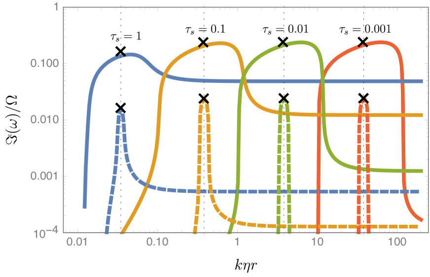
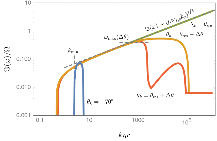
Figure 4: The settling instability (vertical-epicylic RDI)—i.e., the streaming instability including a vertical settling velocity of the dust towards the midplane. The left-hand panel is of the same form as Fig. 3, but includes the settling drift $\mathrm{w}_{s,z}$ from Eq. (3.20) with $\eta=10^{-3}$. The solid curves show $\mu=0.1$, dashed curves show $\mu=0.001$, black crosses show the analytic estimate of the maximum growth rates (Eq. (5.8)), and we take $\theta_{k}=70^{\circ}$ for the mode angle (this angle is chosen so as to show the basic RDI behavior, away from the double-resonant mode). Remarkably, maximum growth rates are large ($\Im(\omega)/\Omega\approx\!\!\sqrt{\mu/2}$, reaching an appreciable fraction of $\Omega$ for larger $\mu$) and independent of the stopping time $\tau_{s}$ (i.e., they are independent of grain size). The vertical settling time is $t_{\mathrm{settle}}\sim 1/(\Omega\,\tau_{s})$, which is much longer than the growth timescale for $\tau_{s}\ll 1$ grains (radial drift timescales are longer still). Also note that the characteristic, maximally unstable wavelengths of the settling instability are larger than the YG streaming instability by a factor $\eta^{-1/2}\sim 30$ (c.f., Fig. 3). The right-hand panel shows the behavior of the mode near the “double-resonant” solution at $\theta_{k}=\theta_{\mathrm{res}}$ when $\bm{k}\cdot{\bf w}_{s}=0$. The solid lines each show numerically calculated dispersion relations with $\mu=0.01$ and $\tau_{s}=0.01$, evaluated at the labeled angles $\theta_{k}=70^{\circ}$ (blue curve), $\theta_{k}=-\theta_{\mathrm{res}}\approx 86.4^{\circ}$ (green curve), $\theta_{k}=\theta_{\mathrm{res}}-0.002\approx\theta_{\mathrm{res}}-0.1^{\circ}$ (red curve), and $\theta_{k}=\theta_{\mathrm{res}}+0.002$ (orange curve). The dashed gray curves illustrate the various analytic results from the text: the growth rate of the double-resonant mode (Eq. (5.16)), the low-$k$ cutoff wavenumber (Eq. (5.17)), and the maximum growth rate (Eq. (5.18)) (i.e., the high-$k$ cut off) for the chosen $\Delta\theta=0.002$. The growth rate of double-resonant modes, at mode angle $\theta_{k}=\theta_{\mathrm{res}}$, increases without bound with $k$ as $\Im(\omega)\propto k^{1/3}$.

It is necessary to account for two changes in our results from §5.2: first, we now have $\mathrm{w}_{s,z}\neq 0$ in the growth rate, Eq. (5.7) or Eq. (5.8); second, $\mathrm{w}_{s,z}\neq 0$ in the resonant condition, $\bm{k}\cdot{\bf w}_{s}=\pm\hat{k}_{z}\,\Omega$, so that Eq. (5.9) is modified to

$$k=\left|\frac{\Omega}{\tan\theta_{k}\mathrm{w}_{s,x}+\mathrm{w}_{s,z}}\right|.$$ (5.11)

For concreteness, we shall consider the $z<0$ region of the disk, where $\mathrm{w}_{s,z}>0$, and set $k_{z}>0$ (i.e., $-\pi/2<\theta_{k}<\pi/2$; results with $\mathrm{w}_{s,z}<0$ are effectively identical). Noting that $|\mathrm{w}_{s,x}|\ll\mathrm{w}_{s,z}>0$, we see that the resonance condition is satisfied for positive-frequency epicycles ($\omega_{\mathcal{F}}=\hat{k}_{z}\Omega$) with $\hat{k}_{x}>0$. We then simply insert the resonant $k$ (Eq. (5.11)) and the drift velocities (Eqs. (3.19)–(3.20)) into the growth rate expression (Eq. (5.7)), and expand in $\tau_{s}\ll 1$ to obtain,

$$\frac{\omega}{\Omega}=\hat{k}_{z}\pm i\left(\frac{\mu}{2}\right)^{1/2}\left(\frac{1+2\eta^{1/2}\cot\theta_{k}}{1-2\eta^{1/2}\tan\theta_{k}}\right)^{1/2}\sin\theta_{k}+\mathcal{O}(\tau_{s},\mu).$$ (5.12)

If we simplify, for the moment, to mode angles where $|k_{x}|\sim k_{z}$, specifically $\eta^{1/2}\ll|\theta_{k}|\ll\pi/2-\eta^{1/2}$, the growth rate of the RDI mode is simply

$$\Im(\omega)\approx\Omega\left(\frac{\mu}{2}\right)^{1/2}\left|\hat{k}_{x}\right|+\mathcal{O}(\tau_{s},\eta^{1/2},\mu)\quad\text{at}\quad k\eta r\approx\frac{\eta^{1/2}}{\tau_{s}},$$ (5.13)

which can also be obtained by setting $\mathrm{w}_{s,x}=\mathrm{w}_{s,y}=0$ in both the resonant condition (Eq. (5.11)) and growth rate (Eq. (5.8); this should be expected, since $|\mathrm{w}_{s,x}|\approx 2\tau_{s}\,\eta U_{K}\ll|\mathrm{w}_{s,z}|\approx\eta^{-1/2}\tau_{s}\,\eta U_{K}$).

While the result (5.13) appears very different to the YG streaming instability, examination of Eq. (5.10) shows that the standard streaming instability does in fact have an $\mathcal{O}(\tau_{s}^{0})$ term in the $\mathcal{O}(\mu^{1/2})$ perturbation to $\omega$: the $(\mu/2)^{1/2}$ term in square brackets in Eq. (5.10). However, this term is purely real when $\mathrm{w}_{s,z}=0$. In contrast, when a vertical streaming dominates the drift velocity, the symmetry that caused this term to be real is broken, and the instability has a $\tau_{s}$-independent part. In the left panel of Fig. 4, which is of the same form as Fig. 3, we compare the numerically calculated growth rates to the analytic expression (Eq. (5.7)) for a variety of $\tau_{s}$ and $\mu$.

Examining the eigenmodes of the settling instability, we see that the linear mode contains a substantial dust density perturbation. This is also the case for the YG streaming instability, and, in fact, must be true for any instability in the RDI family, because RDIs arise due to the gas wave resonance with the density perturbation of the dust (see §4). The size of the dust density perturbation (compared to other components of the eigenmode) scales as $\mu^{-1/2}$: thus, at decreasing grain concentrations, the relative perturbation of the dust density increases, more directly seeding large dust-to-gas ratio fluctuations without stirring up the gas. This behavior is expected and very similar to that seen in other RDIs (see, e.g., §3.9 of HS17 for further discussion).

5.3.1 The double-resonant $\theta_{k}$

A careful examination of Eqs. (5.11) and (5.12) uncovers an interesting effect that is not captured by Eq. (5.13): the resonant wavenumber and growth rate approach infinity as $\bm{k}\cdot{\bf w}_{s}$ approaches zero (or equivalently $2\eta^{1/2}\tan\theta_{k}$ approaches $1$). This can also be seen in the full RDI expression, Eq. (5.8), which increases as $k_{\mathrm{res}}$ increases, but does not contain $\bm{k}\cdot{\bf w}_{s}$ in the numerator. As we now show, at this “double-resonant” angle,

$$\theta_{\mathrm{res}}=\arctan\left(-\frac{\mathrm{w}_{s,z}}{\mathrm{w}_{s,x}}\right)\approx\arctan\left(\frac{1}{2\eta^{1/2}}\right)\approx 86^{\circ}\text{ (at }\eta=10^{-3}),$$ (5.14)

the growth rate increases without bound with $k$, scaling as $\Im(\omega)/\Omega\!\sim\!\mu^{1/3}\tau_{s}^{1/3}k^{1/3}$ (of course, we are neglecting viscosity, turbulence, and other dissipative effects; see §8). Although we derive its properties here in an unstratified incompressible gas, this mode survives the addition of dust and gas stratification and a compressible treatment (see §6.3). The numerically calculated dispersion relation is shown in the right-hand panel of Fig. 4 for a variety of angles near $\theta_{k}=\theta_{\mathrm{res}}$.

Properties of the double-resonant mode are simplest to derive from the dispersion relation for the full coupled dust-gas system. This is found from the matrix operators, Eqs. (5.1)–(5.4), as the characteristic polynomial of $\mathbb{T}_{0}+\mu\mathbb{T}^{(1)}$ (Eqs. (4.1)–(4.2)) after inserting $\bm{k}\cdot{\bf w}_{s}=0$. We then insert the ansatz $\omega/\Omega=\varpi\,\mu^{1/3}\tau_{s}^{1/3}(k\eta r)^{1/3}$, insert equation (3.19) for ${\bf w}_{s}$, and expand in high $k$ ($k\eta r\sim\epsilon^{-1}$) and small $\mu$ and $\tau_{s}$ ($\mu\sim\epsilon^{\nu}$, $\tau_{s}\sim\epsilon^{1-\nu}$, with $0<\nu<1$), yielding the polynomial,

$$\varpi^{3}-\varpi\frac{\cos^{2}\!\theta_{k}}{(\mu\,\tau_{s}\,k\eta r)^{2/3}}+2\sin\theta_{k}=0.$$ (5.15)

When $\omega/\Omega=\varpi\mu^{1/3}\tau_{s}^{1/3}(k\eta r)^{1/3}\gg\cos\theta_{k}$, the middle term in Eq. (5.15) is negligible, giving the unstable root,

$$\frac{\omega}{\Omega}\approx\frac{1}{2}(-1+i\sqrt{3})(2\tau_{s}\,\mu\,k_{x}\eta r)^{1/3},$$ (5.16)

which justifies our original ansatz for $\omega$ and shows that $\Im(\omega)\rightarrow\infty$ as $k\rightarrow\infty$. The middle term in equation (5.15) is important when $\omega/\Omega\lesssim\cos\theta_{k}\approx\pi/2-|\theta_{k}|$. This gives the minimum wavenumber for which the solution (5.16) is valid,

$$k_{\mathrm{min}}\eta r\sim\frac{(\pi/2-|\theta_{\mathrm{res}}|)^{3}}{\mu\,\tau_{s}},$$ (5.17)

which is shown in the lower panel of Fig. 4. We note that this estimate for $k_{\mathrm{min}}$ is modified in the presence of gas stratification, because the gas oscillations are modified; see §§6.3.4–6.3.5 and Eq. (6.17).

In addition to dissipative effects not included here (see §9), the instability is cut off at high wavenumbers due to misalignment of $\theta_{k}$ from $\theta_{\mathrm{res}}$. Because in reality (or numerical simulations) not all mode angles are necessarily possible, it is helpful to understand how this cutoff scales with the misalignment $\Delta\theta=\theta_{k}-\theta_{\mathrm{res}}$. To do this, we recalculate the dispersion relation from $\mathbb{T}_{0}+\mu\mathbb{T}^{(1)}$, but now with $\bm{k}\cdot{\bf w}_{s}=\kappa\,k\,\tau_{s}$, where $\kappa\sim-\eta^{-1/2}\Delta\theta$ is a small parameter. Repeating the expansion described above using the same ordering and $\kappa\,\tau_{s}\sim 1$ yields the additional terms $(\kappa/\mu)\cos^{2}\theta_{k}+(\kappa/\mu)(\mu\,\tau_{s}k\eta r)^{2/3}\varpi^{2}$ in equation (5.15). The former term has no effect, but the latter term is important to the solutions for $\varpi$ unless $(\kappa/\mu)(\mu\,\tau_{s}k\eta r)^{2/3}\ll 1$. Asserting that this term be negligible, we obtain the cutoff growth rate,

$$\frac{\omega_{\mathrm{max}}}{\Omega}\sim\left(\frac{\mu\,\eta^{1/2}}{|\Delta\theta|}\right)^{1/2}.$$ (5.18)

In the lower panel of Fig. 4, we also show modes with $\theta_{k}=\theta_{\mathrm{res}}\pm 0.002$, illustrating nice agreement with equation (5.18). The cutoff in Eq. (5.18) also helps to clarify the connection between the double-resonant solution (Eq. (5.16)) and the RDI solution (Eq. (5.12)): as $\theta_{k}$ approaches $\theta_{\mathrm{res}}$ (from below $|\theta_{k}|<|\theta_{\mathrm{res}}|$), the predicted RDI growth rate, obtained by expanding Eq. (5.12) in $\theta_{k}$ about $\theta_{\mathrm{res}}$, is $\Im(\omega)=(\mu\,\eta^{1/2}/|\Delta\theta|)^{1/2}\sin\theta_{k}$. This matches the cutoff growth rate of the double-resonant mode (Eq. (5.18)). Put differently, the RDI solution in Eq. (5.12) correctly predicts the maximum of $\Im(\omega)$, although it cannot predict the $\Im(\omega)\sim k^{1/3}$ scaling of the double-resonant mode.

6 Gas stratification

In the previous section, we studied the YG streaming instability and epicyclic RDI more generally. The most interesting result of this section was that the instability becomes significantly faster-growing when the dust also undergoes vertical streaming motion (i.e., settling towards the midplane of the disk)—a new instability that we termed the “settling instability.” However, those regions of the disk away from the midplane are also stratified, which (if stable) allows for buoyancy oscillations that can cause another RDI (the Brunt-Väisälä RDI). With this in mind, the purpose of this section is twofold: first, we examine the resonance with Brunt-Väisälä (BV) oscillations and the resulting instability; second, we verify that the behavior of the disk settling instability described in §5.3 is robust to the addition of gas/dust stratification and compressibility. To do this, we derive the “vertical-epicyclic-Brunt-Väisälä RDI,” which results from the resonance with joint epicyclic-BV oscillations in the gas. The properties of this RDI are very similar to the pure epicyclic RDI, so, in the astrophysical discussion of §9, we will simply term this RDI the disk settling instability also.

After introducing useful variables and the local formulation in §6.1, we shall examine a simple stratified fluid (i.e., without rotation) in §6.2. This allows us to better understand the properties of the resulting Brunt-Väisälä (BV) RDI, which was briefly introduced in SH17, without undue complications. This instability may be interesting in its own right for other (non-disk) applications and has likely been observed in previous numerical simulations (Lambrechts et al., 2016; see §9.3). We then treat the full, stratified, rotating, compressible problem in §6.3, deriving the epicyclic-BV RDI, illustrating how this reduces to the epicyclic and BV RDIs separately in the relevant limits (i.e., both the pure epicyclic and BV RDIs are special cases of the epicyclic-BV RDIs), and discussing the influence of stratification on the disk settling instability (§6.3.5).

Finally, we note that, formally, the local treatment of background gradients used throughout this section may not be appropriate. In principle, for this problem, it may be necessary to embark on a fully global treatment or a spatially dependent WKBJ expansion (Bender & Orszag, 1978; White, 2010), which is quite complicated and beyond the scope of this work. While this could potentially yield corrections to the growth rates presented here (e.g., from second-order gradients of background quantities), it is likely that the local treatment correctly captures most aspects of the Brunt-Väisälä and vertical-epicyclic-BV RDIs. In any case, the main purpose of this section is to show that the stratification has only a relatively weak effect on the settling instability in disks, and, given the uncertainty that surrounds the actual stratification profile in disks, nonlinear simulations are obviously required to study the instability in significantly more detail. Brief discussion of these mathematical issues is given below in §6.1.1.

6.1 The linear system to be solved

We shall examine a local patch of disk with an arbitrary background pressure and temperature gradient in the $\hat{\bm{x}}$ (radial) and $\hat{\bm{z}}$ (vertical) directions. The fluid equations are Eqs. (3.1)–(3.2) with the pressure gradient balancing the combination of gravity ($\bm{g}=g\hat{\bm{g}}$) and the drag force parallel to $\bm{g}$; i.e., $\rho_{0}^{-1}\nabla P_{0}=-\mu({{\bf w}_{s}\cdot\hat{\bm{g}}})/{t_{s0}}\,\hat{\bm{g}}+\bm{g}$. As described above (see §3.4 and HS17), an additional force perpendicular to $\hat{\bm{g}}$ (e.g,. from radiation pressure on the grains) could in principle cause a perpendicular ${\bf w}_{s}$ also, accelerating the dust and gas together once the dust reaches its terminal velocity (the analysis is then carried out in the free-falling frame). Thus, in our derivation of the Brunt-Väisälä (BV) RDI in §6.2, we allow for a nonzero perpendicular drift for completeness.

Rather than the pressure $P$ (Eq. (3.3)), it is easier to work with the entropy, $S\equiv\gamma_{\mathrm{gas}}^{-1}\ln(P/\rho^{\gamma_{\mathrm{gas}}})$, which evolves according to ${\partial_{t}S}+\bm{u}\cdot\nabla S=0$. The gas equilibrium is then determined by $\bm{g}$, $P_{0}$ and $\rho_{0}$ (through $c_{s0}^{2}=\gamma_{\mathrm{gas}}P_{0}/\rho_{0}$), and $\nabla S_{0}$, and it is helpful to define the following variables to describe this:

$$L_{0}^{-1}\equiv\gamma_{\mathrm{gas}}^{-1}\,\frac{1}{P_{0}}\,\frac{\partial P_{0}}{\partial z},\quad L_{0R}^{-1}\equiv\gamma_{\mathrm{gas}}^{-1}\,\frac{1}{P_{0}}\,\frac{\partial P_{0}}{\partial r}\sim\eta^{1/2}L_{0}^{-1},$$

$$c_{s0}=\gamma_{\mathrm{gas}}\frac{P_{0}}{\rho_{0}},\quad\tilde{\bm{g}}\equiv\frac{1}{\rho_{0}}\nabla P_{0}=c_{s0}^{2}(L_{0R}^{-1}\,\hat{\bm{x}}+L_{0}^{-1}\,\hat{\bm{z}}),$$

$$-\Lambda_{S}\equiv{L_{0}}\frac{\partial S_{0}}{\partial z}\approx{L_{0R}}\frac{\partial S_{0}}{\partial r}.$$ (6.1)

In these definitions, we have neglected a background dust density or ${\bf w}_{s}$ stratification, which is treated in App. B and results in minor modifications to the RDI growth rates. We also assume for simplicity that the stratification direction of $S_{0}$ is the same as that of $P_{0}$ (i.e., we need only the parameter $\Lambda_{S}$, rather than a separate parameter for the vertical and radial directions separately). Relaxing this assumption does not fundamentally modify the RDIs studied here, but can also lead to baroclinic instabilities, which we do not wish to study (see, e.g., Klahr & Hubbard 2014; Lorén-Aguilar & Bate 2016; Lin & Youdin 2017). The definitions in equation (6.1) give $\nabla\ln\rho_{0}=(L_{0R}^{-1}\,\hat{\bm{x}}+L_{0}^{-1}\,\hat{\bm{z}})\,(1+\Lambda_{S})$ and yield the vertical Brunt-Väisälä frequency $N_{BV}^{2}=c_{s0}^{2}(L_{0}^{-2}+L_{0R}^{-2})\,\Lambda_{S}$ (see below). Note that, because we expand in $\mu$ to $\mathcal{O}(\mu^{1/2})$, there is no need to distinguish between $\bm{g}$ and $\tilde{\bm{g}}=-\mu({{\bf w}_{s}\cdot\hat{\bm{g}}})/{t_{s0}}\,\hat{\bm{g}}+\bm{g}$ in our analytic analysis below (the full terms are retained in our numerical solutions). For concreteness, we shall set $L_{0}>0$, as appropriate for regions below the midplane. The natural direction for the settling velocity—i.e., dust streaming towards the midplane—is thus $\mathrm{w}_{s,z}>0$, as used in §5.3 (regions above and below the midplane behave identically, we specify the direction only for notational clarity).

We construct the local equations by taking $k_{z}L_{0}\gg 1$ and $k_{x}L_{0R}\gg 1$, and assuming the background gradients of $P_{0}$, $S_{0}$, and $\rho_{0}$ are constant so as to Fourier analyze the equations in the $x$ and $z$ directions. This is nearly equivalent to a formal WKBJ expansion to lowest order in $(kL_{0})^{-1}$, and is discussed in more detail below (§6.1.1). Also assuming axisymmetric perturbations ($k_{y}=0$), we obtain the linearized gas and dust equations,

$$-i\omega\frac{{\delta\rho}}{\rho_{0}} +i\bm{k}\cdot\delta\bm{u}+\delta\bm{u}\cdot(L_{0R}^{-1}\hat{\bm{x}}+L_{0}^{-1}\hat{\bm{z}})\,(1+\Lambda_{S})=0,$$ (6.2)

$$-i\omega\delta\bm{u} =-ic_{s0}^{2}\bm{k}\left(\delta S+\frac{\delta\rho}{\rho_{0}}\right)+\frac{\delta\rho}{\rho_{0}}\tilde{\bm{g}}+\frac{3}{2}\Omega\delta u_{x}\hat{\bm{y}}$$

$$-2\Omega\hat{\bm{z}}\times\delta\bm{u}-\mu\frac{\delta\bm{u}-\delta\bm{v}}{t_{s0}}+\mu\frac{{\bf w}_{s}}{t_{s0}}(\delta t_{s}+\frac{\delta\rho}{\rho_{0}}-\frac{\delta\rho_{d}}{\rho_{d0}}),$$ (6.3)

$$-i\omega\delta S -\delta\bm{u}\cdot(L_{0R}^{-1}\hat{\bm{x}}+L_{0}^{-1}\hat{\bm{z}})\,\Lambda_{S}=0,$$ (6.4)

$$(-i\omega+ i\bm{k}\cdot{\bf w}_{s})\frac{{\delta\rho_{d}}}{\rho_{d0}}+i\bm{k}\cdot\delta\bm{v}=0,$$ (6.5)

$$(-i\omega+ i\bm{k}\cdot{\bf w}_{s})\,\delta\bm{v}=-2\Omega\hat{\bm{z}}\times\delta\bm{v}+\frac{3}{2}\Omega\delta v_{x}\hat{\bm{y}}-\frac{\delta\bm{v}-\delta\bm{u}}{t_{s0}}-{\bf w}_{s}\frac{\delta t_{s}}{t_{s0}}.$$ (6.6)

As appropriate for subsonic streaming velocities ${w}_{s}\ll c_{s0}$, we neglect the velocity dependence of $t_{s}$, taking $\delta t_{s}/t_{s0}=-\zeta_{\rho}\,\delta{\rho}/\rho_{0}-\zeta_{P}\,\delta{P}/P_{0}=-(\zeta_{\rho}+\gamma_{\mathrm{gas}}\zeta_{P})\,\delta{\rho}/\rho_{0}-\gamma_{\mathrm{gas}}\zeta_{P}\,\delta{S}$.

6.1.1 A cautionary note about the local approximation

As mentioned in the introduction above, caution should be used in interpreting the solutions to Eqs. (6.2)–(6.6), because it is possible that there are neglected terms that could modify the growth rate. In this section we briefly discuss this subtlety, and how it can be remedied in future work. Those readers uninterested in these somewhat esoteric mathematical details should feel free to skip to §6.2.

Formally, a local “dispersion relation” should be derived from the linearized fluid equations through a WKBJ expansion, without assuming anything about the background $\rho_{0}(\bm{x})$, $P_{0}(\bm{x})$. This involves expanding in $\epsilon\sim(kL_{0})^{-1}$, assuming that the linear fields ($\delta\rho$, $\delta\bm{u}$, etc.) have the form $\exp[i\,\epsilon^{-1}\sum_{i=0}^{\infty}\epsilon^{j}Q_{j}(\bm{x})]$. The lowest-order expression in $\epsilon$ yields a “dispersion relation”: more formally, a local relationship between $\nabla Q_{0}$ and $\omega$, which (for a given $\omega$) specifies how the wavelength varies with background quantities. For example, applying such a procedure to a pure stratified gas (i.e., Eqs. (3.1)–(3.3) with $\mu=0$), one finds either the Brunt-Väisälä dispersion relation or the sound-wave dispersion relation, depending on the choice for the asymptotic scaling of $\omega$ (i.e., the choice of dominant balance). The $\omega$ one obtains, and the eigenmodes—i.e., the local relationship between $\delta\rho(\bm{x})$, $\delta\bm{u}(\bm{x})$, and $\delta S(\bm{x})$—are identical, at lowest order in $(kL_{0})^{-1}$, to those obtained through an expansion of the local equations (Eqs. (6.2)–Eqs (6.4) with $\mu=0$). These are also identical to a standard (unstratified) sound wave, and an analysis using the Boussinesq approximation (indeed, this amounts to a formal derivation of the linear Boussinesq approximation). However, this exact agreement between the local and formal WKBJ result is only valid at lowest order in $(kL_{0})^{-1}$, and it is not logically consistent to expand the local solutions (Eqs. (6.2)–(6.3)) to higher order. More precisely, while the the WKBJ dispersion relation is unmodified at the next order $(kL_{0})^{-1}$ in the WKBJ expansion (more generally, the dispersion relation is only modified at every second order in $\epsilon$; see Bender & Orszag 1978), the WKBJ eigenmodes have corrections that appear at order $(kL_{0})^{-1}$.

In the coupled dust-gas system, the potential for a problem arises because ${w}_{s}/c_{s}$ is also a small parameter, which is of the same order as $(kL_{0})^{-1}$ (this must be the case due to the resonance condition; see Eq. (6.9) below). As will become clear below, this mixes the $\mathcal{O}[(kL_{0})^{-1}]$ correction to the eigenmodes—which is not captured correctly by Eqs. (6.2)–(6.4)—into the lowest-order result for the RDI, and may cause the RDI growth rate to depend on, for instance, second derivatives of $P_{0}$ and $\rho_{0}$. However, it is also possible that the resonant-mode growth rates derived from Eqs. (6.2)–(6.6) are correct, if the intuition above—that the lowest-order WKBJ dispersion relation is captured correctly by the local equations—also holds for this much more complicated coupled dust-gas system. Unfortunately, checking this explicitly is not a trivial task, and is beyond the scope of this work. We will address this issue in future work with a fully global analysis.

One clear regime of validity for our results, and for Eqs. (6.2)–(6.6) in general, is that $\mu$ must be sufficiently large such that the perturbation on the gas modes from the dust is larger than the higher-order WKBJ corrections. Equivalently, noting that the correction to the Brunt-Väisälä (or epicyclic-BV) mode arises at $\mathcal{O}[(kL_{0})^{-2}]$, the perturbed eigenmode ($\omega^{(1)}$) should satisfy $\omega^{(1)}\gtrsim(kL_{0})^{-2}N_{BV}$, which becomes $\mu^{1/2}\gtrsim(kL_{0})^{-1}$ using Eq. (6.11) below (this can also be seen directly from the gas-dust equations, noting that the RDI theory of §4 shows that $\omega^{(1)}$, the $\mathcal{O}(\mu^{1/2})$ correction to $\omega$, depends only on the coupling of dust to gas). This condition is not particularly stringent, and well satisfied for smaller grains in disks (see §9.3 for further discussion).

Finally, it is worth noting that the Brunt-Väisälä RDI has likely already been seen in simulations in Lambrechts et al. (2016). As discussed in §9.3.1, the observed growth rates are comparable to our predictions, although a detailed comparison is not possible.

6.2 Brunt-Väisälä RDI

In this section, we treat a stratified fluid in the absence of rotation. As discussed above, while this situation is not directly applicable to thin disks (the rotation is always dynamically important), the treatment is helpful to isolate the different character of the RDI that arises due to Brunt-Väisälä (BV) oscillations. As we show below (§6.3), the instability is effectively a special case of the joint epicyclic-BV RDI for $\Omega=0$. We consider Eqs. (6.2)–(6.6) without the influence of rotation ($\Omega=0$), also setting $L_{0R}=0$ because the stratification direction is arbitrary if $\Omega=0$. However, even though we set $\Omega=0$ in the dynamical equations, for clarity and consistency with the rest of the paper, we quote results in terms of $\tau_{s}=t_{s}\Omega$ (i.e., $\Omega$ is effectively an arbitrary frequency scale) and the pressure support parameter $\eta$. Thus we consider a vertical stratification profile appropriate for a disk, with $L_{0}\sim h_{g}\sim\eta^{1/2}r$ and $c_{s0}\sim h_{g}\Omega$, leading to the natural scaling for the settling drift velocity (in the absence of an external acceleration on the dust), ${\bf w}_{s}\approx\tau_{s}c_{s0}\hat{\bm{z}}$ (see §3.5). Preemptively noting that the resonance condition gives ${w}_{s}/c_{s}\sim(k_{\mathrm{res}}L_{0})^{-1}$, as well as the fact that $(kL_{0})^{-1}\ll 1$ is required for any sort of local treatment, our analysis shall proceed by expanding all expressions in $\epsilon\ll 1$, with $\epsilon\sim\tau_{s}\sim(kL_{0})^{-1}\sim{w}_{s}/c_{s0}$. As discussed above, we require $\mu^{1/2}\gg\epsilon$ for the consistency of the expansion.

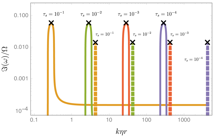
Figure 5: Illustration of the growth rate $\Im(\omega)$ of the pure Brunt-Väisälä RDI including compressibility but neglecting disk rotation. This is a distinct dust-gas instability which arises from resonance with BV oscillations. Each curve is calculated through numerical solution of the local dispersion relation from Eqs. (6.2)–(6.6) with $\Omega=0$, and uses $\mu=0.01$, Epstein drag ($\zeta_{\rho}=\zeta_{P}=1/2$), stratification parameter $\Lambda_{S}=2$, equation-of-state $\gamma_{\mathrm{gas}}=5/3$, and $\tau_{s}$ as labeled (orange curves, $\tau_{s}=0.1$; green curves, $\tau_{s}=0.01$; red curves, $\tau_{s}=10^{-3}$; purple curves, $\tau_{s}=10^{-4}$). Even though rotation is not included in the calculation, we use disk units (§3.3) to allow direct comparison to other figures, taking the vertical pressure scale-length $L_{0}=h_{g}\approx\eta^{-1/2}(\eta r)$ and sound speed $c_{s0}=\eta^{-1/2}(\eta U_{K})$ with $\eta=0.001$ (ignoring the radial pressure-scale length, i.e. $L_{0R}^{-1}=0$, because the geometry here is arbitrary). The solid curves show $\Im(\omega)$ including the vertical settling drift of the dust (Eq. (3.20)), while dashed curves show $\Im(\omega)$ with $\mathrm{w}_{s,z}=0$ (only radial/azimuthal drift) for comparison. For both cases, we take the mode angle to be $\hat{k}_{x}=\hat{k}_{z}$ ($\theta_{k}=\pi/4$), which maximizes the growth rate for the $\mathrm{w}_{s,z}=0$ RDI (with the settling drift included, the growth rate is maximized near $\theta_{k}=\pi/2$). The maximum growth rates reach an appreciable fraction of $\Omega$ (even at low dust-to-gas ratios) and are independent of grain size ($\tau_{s}$), although the resonance is narrower in wavenumber compared to the (disk) settling instability shown in Fig. 4.

6.2.1 Gas oscillations

With $\mu=0$ (i.e., no dust), Eqs. (6.2)–(6.4) have five eigenmodes: $\omega=0$ (this represents an undamped zonal flow in $u_{y}$), two sound-wave eigenmodes, with

$$\omega_{\mathcal{F}}=\pm\epsilon^{-1}c_{s0}\,k+\dots$$ (6.7)

and two BV eigenmodes,

$$\omega_{\mathcal{F}}=\pm\hat{k}_{x}N_{BV}+\dots,$$ (6.8)

where $N_{BV}^{2}=\Lambda_{S}c_{s0}^{2}L_{0}^{-2}$ is the BV frequency. We focus on resonance with the BV modes (Eq. (6.8)) and refer to HS17 App. C for an analysis of stratified sound waves, which introduce their own, additional RDIs (the acoustic RDI, discussed separately below). The BV modes are stable so long as $\Lambda_{S}>0$ and represent slow (compared to sound waves) oscillations, with the restoring force provided by buoyancy. As expected, the BV eigenmode is approximately incompressible, $\bm{k}\cdot\delta\bm{u}\approx 0$ to lowest order in $\epsilon$, and the density fluctuations dominate over pressure fluctuations (i.e., $\delta\rho/\rho_{0}+\delta S\approx 0$). This is the linear manifestation of the the Boussinesq approximation, which stipulates $\nabla\cdot\delta\bm{u}\approx 0$ and $\delta\rho/\rho_{0}\approx-\delta T/T_{0}$ (where $\delta T/T_{0}$ is the relative temperature fluctuation). At next order in $\epsilon\sim(kL_{0})^{-1}$, the BV eigenmode has a small compressive component (the form of this can be found, for example, from a WKBJ analysis; see §6.1.1)

6.2.2 Resonant drag instability

A BV RDI can occur when the drift frequency $\bm{k}\cdot{\bf w}_{s}$ matches the BV oscillation frequency, viz., at the resonant wavenumber,

$$k_{\mathrm{res}}\approx\pm\frac{\sin\theta_{k}N_{BV}}{\hat{\bm{k}}\cdot{\bf w}_{s}}=\frac{c_{s0}}{{w}_{s}}\Lambda_{S}^{1/2}L_{0}^{-1}\frac{\sin\theta_{k}}{\hat{\bm{k}}\cdot\hat{{\bf w}}_{s}}.$$ (6.9)

We see, as mentioned earlier, that $(k_{\mathrm{res}}L_{0})^{-1}\sim{w}_{s}/c_{s}$, justifying the $\epsilon$ ordering used for the expansion. In the same way as for the derivation of the streaming instability in §5.1, we then insert the eigenmodes corresponding to BV oscillations (Eq. (6.8)) into the RDI growth rate formula (Eq. (4.3)), to obtain an expression for the growth rate of the BV RDI at $k=k_{\mathrm{res}}$. For the positive frequency BV mode this yields (to lowest order in $\epsilon$), $\omega=\hat{k}_{x}N_{BV}+\omega^{(1)}$ with

$$(\omega^{(1)})^{2}=\mu\frac{\zeta_{\rho}N_{BV}\,(\hat{\bm{k}}\cdot{\bf w}_{s})\,(\hat{\bm{k}}\times{\bf w}_{s})_{y}}{2c_{s0}^{2}t_{s0}}(k_{\mathrm{res}}L_{0})+\mu\frac{\hat{k}_{x}N_{BV}(\hat{\bm{k}}\times{\bf w}_{s})_{y}}{2c_{s0}t_{s0}\sqrt{\Lambda_{S}}},$$ (6.10)

or, inserting $k_{\mathrm{res}}$ from Eq. (6.9),

$$\omega\approx\hat{k}_{x}N_{BV}+\mu^{1/2}\left[\frac{\hat{k}_{x}(\hat{\bm{k}}\times{\bf w}_{s})_{y}}{2t_{s0}L_{0}}\Theta_{S}\right]^{1/2},$$ (6.11)

where $\Theta_{S}=1+\zeta_{\rho}\Lambda_{S}$. The $\zeta_{\rho}\Lambda_{S}$ term in $\Theta_{S}$ arises from the lowest-order (Boussinesq) contribution to the gas BV eigenmode. Because this part of the oscillation is incompressible, the contribution to the RDI depends directly on the dependence of $t_{s}$ on $\delta\rho$ (through $\zeta_{\rho}$). The $1$ term in $\Theta_{S}$ arises from the next-order (in $\epsilon\sim(kL_{0})^{-1}$) contribution to the BV eigenmode, and has entered at the same order in the RDI growth rate because this compressible part of the BV oscillation interacts more strongly with the dust. As discussed above in §6.1.1, the exact form of this contribution could be modified (e.g., by second derivatives of the background) if a true WKBJ treatment is carried out, and this value should be treated with some skepticism. However, the general physical picture—that the instability is enhanced due to the interaction with the compressive part of the BV mode—is likely quite general, because the first-order compressive part of the BV eigenmode (the correction to $\delta\rho$) is correctly captured by Eqs. (6.2)–(6.6). This picture also fits well into the toy model outlined in §1.2 and Fig. 1, in which gas pressure perturbations play a particularly important role in the RDI’s mechanism. The global analysis necessary to treat this compressive contribution more formally will be considered in future work.

As shown in App. B, the addition of dust and/or ${\bf w}_{s}$ stratification causes the $\Theta_{S}=1+\zeta_{\rho}\Lambda_{S}$ factor to become $1+\zeta_{\rho}\Lambda_{S}-\Lambda_{\rho_{d}}$, where $\Lambda_{\rho_{d}}=L_{0}^{-1}d\ln\rho_{d0}/dz$ (this result is again subject to the caveats of the local model outlined in §6.1.1; see also App. C of HS17).

6.2.3 Properties of the Brunt-Väisälä RDI

It is worth briefly commenting on some properties on the BV RDI, Eq. (6.11), and how this depends on the sign of the $\Theta_{S}=1+\zeta_{\rho}\Lambda_{S}$ factor (or, more precisely, whatever modified version of $\Theta_{S}$ appears due to dust stratification or a more formal WKBJ treatment). Noting that $(\hat{\bm{k}}\times{\bf w}_{s})_{y}=\hat{k}_{z}\mathrm{w}_{s,x}-\hat{k}_{x}\mathrm{w}_{s,z}$, and that the term in square brackets in Eq. (6.11) must be negative to cause an RDI, we see that when $\Theta_{S}>0$ and $\mathrm{w}_{s,x}\ll\mathrm{w}_{s,z}$, an RDI occurs if $\mathrm{w}_{s,z}$ and $\nabla\ln P_{0}$ (or $\nabla\ln\rho_{0}$) have the same sign. This is the “natural” direction for particles to drift when the gas is pressure supported and dust is not, i.e., in the direction of gravity, towards the midplane of the disk. In contrast, if $\Theta_{S}<0$, the RDI is most unstable when $\nabla\ln P_{0}$ and $\mathrm{w}_{s,z}$ have opposite signs, viz., when the dust in streaming in the direction opposite to gravity (this case is of course less physical but could occur, e.g., due to radiation pressure or another external force). If the dust has a substantial drift perpendicular to the stratification direction ($\mathrm{w}_{s,x}\sim\mathrm{w}_{s,z}$), the BV RDI growth rate is comparable for either $\Theta_{S}>0$ or $\Theta_{S}<0$ (with different signs of $\hat{k}_{x}$).

Assuming, for the sake of discussion, that we have little dust stratification ($\Lambda_{\rho_{d}}\lesssim 1$) and that the possible corrections to $\Theta_{S}$ in a more formal WKBJ treatment are minor, we see that the sign of $\Theta_{S}$ depends primarily on the drag regime (Epstein or Stokes). Because $\Lambda_{S}>0$ for the system to be hydrodynamically stable, grains in the Epstein regime ($\zeta_{\rho}\approx 1/2$) always satisfy $\Theta_{S}>0$ and so are unstable when ${\bf w}_{s}$ and $\nabla P_{0}$ have the same orientation. As discussed further below in §9.3, this makes the BV RDI rather generic: it will occur whenever grains settle through a stratified atmosphere (see also Lambrechts et al., 2016). Grains in the Stokes regime, with $\zeta\approx-1/2$ can cause $\Theta_{S}$ to have either sign, depending on the strength of the entropy stratification $\Lambda_{S}$, so the instability will be slower growing and less generic for these larger grains. We illustrate the behavior of the dispersion relation as $\Theta_{S}$ flips sign in Fig. 10.

Finally, it is worth reiterating that our treatment here has suggested that the BV RDI is somewhat more robust, and faster growing, than predicted using the Boussinesq approximation (albeit with the caveats that come with assuming linear background gradients; see §6.1.1). This occurs because gas pressure perturbations are particularly important to the mechanism of the RDI (see §1.2), but these are neglected in the Boussinesq treatment of BV oscillations. The two results agree for a gas that is very stably stratified, with $\Lambda_{S}\gg 1$ (e.g., strong temperature stratification in the direction opposite to the density stratification).

6.3 Stratified epicyclic instability (the Settling Instability including stratification)

In this section, we calculate the RDI for the full stratified, rotating system. As discussed above, this procedure yields an instability that is, in most regimes, very similar to the pure vertical-epicyclic RDI (§5.3), and we shall also term this instability the disk “settling instability.” Despite the complexity of the equations, we derive a relatively compact expression for the vertial-epicyclic-BV RDI to lowest order in $\tau_{s}$. The primary purpose of this derivation is to highlight the relevance of the results derived in §5 and §6.2. In particular, we find that the RDI of the full system—including joint epicyclic-BV gas oscillations, gas compressibility, a general dust drag law, and dust and gas stratification—behaves very similarly to the unstratified epicyclic RDI (settling instability; §5), with a slightly larger growth rate. We shall also see that the double-resonant behavior studied in §5.3.1, which caused the streaming instability growth rate to approach $\infty$ at $k\rightarrow\infty$, is not pathological; i.e., the fast growth rates of the disk settling instability still exist in stratified regions of disks where the vertical streaming velocity has a clear physical origin.

The same caveats regarding the local approximation apply here, specifically to those terms in the epicyclic-BV RDI that arise from directly from the gas stratification. In particular, as outlined in §§6.1.1 and 6.2.3, the $\Theta_{S}$ term may be modified in a more formal WKBJ treatment. However, since this causes only minor modifications to the settling instability growth rate, any minor modifications to $\Theta_{S}$ would have little effect on our general conclusions.

For simplicity, we shall neglect radial stratification in our analytic derivations below; i.e., we set $L_{0R}^{-1}=0$ in Eqs. (6.2)–(6.6). In numerical results (i.e., Fig. 6), we include a radial stratification $\partial_{r}\ln P_{0}=\eta^{1/2}\partial_{z}\ln P_{0}$ and note that it makes very little difference to the results, because the BV RDI depends only weakly on slight differences between the streaming direction and stratification direction so long as $\Theta_{S}=1+\zeta_{\rho}\Lambda_{S}>0$ (see §6.2.3).

6.3.1 Expansion in $\tau_{s}$

As in §6.2, we carry out the expansion in $\epsilon\sim\tau_{s}$, which incorporates the smallness of $(kL_{0})^{-1}$ and ${w}_{s}/c_{s}$ (specifically ${w}_{s}/c_{s}\sim(kL_{0})^{-1}\sim\tau_{s}\sim\epsilon\ll 1$) and leads to relatively simple and physically intuitive expressions that are easily analyzed. We do not feel that this restriction to $\tau_{s}\ll 1$ is a severe limitation on the applicability of our results: grains with $\tau_{s}\sim 1$ settle out of stratified regions quickly with velocities approaching the sound speed (see §3.5), so are more naturally treated in the midplane region anyway (i.e., the YG streaming instability; see e.g., Fig. 3).

The expected drift velocity from Eqs. 3.19–(3.20), is

$$\frac{{\bf w}_{s}}{c_{s0}}\approx(-2\eta^{-1/2}\tau_{s},\,\eta^{-1/2}\tau_{s}^{2},\,\tau_{s})+\mathcal{O}(\tau_{s}^{3}).$$ (6.12)

To lowest order in $\tau_{s}$, this motion is simply due to the gas stratification, viz., it is the grain settling drift that would arise in a stationary gas with the pressure stratification that we have assumed for the disk ($\partial_{r}\ln P_{0}\sim\eta^{1/2}\partial_{z}\ln P_{0}$).

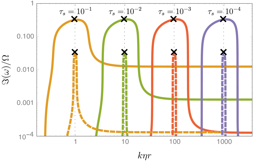
Figure 6: Illustration of the growth rate $\Im(\omega)$ of the vertical-epicyclic-Brunt-Väisälä RDI (settling instability including gas stratification), which arises from the resonance of the dust with epicyclic-Brunt-Väisälä oscillations of the gas. The calculation includes gas compressibility and stratification in the vertical and radial directions. All curves are calculated through numerical solution of the local dispersion relation from Eqs. (6.2)–(6.6), and use $\eta=0.001$ and $c_{s0}=\eta^{-1/2}(\eta U_{K})$, $L_{0}=h_{g}=\eta^{-1/2}(\eta r)$, $L_{0R}=\eta^{-1/2}L_{0}$, $\Lambda_{S}=2$, $\zeta_{\rho}=\zeta_{P}=1/2$ (Epstein drag), and $\gamma_{\mathrm{gas}}=5/3$. The left-hand panel is of the same form as Fig. 3 and the left panel of Fig. 4, and shows the numerically calculated growth rate (curves) and analytic result (Eq. (6.16); crosses) for a range of dust sizes as labeled: $\tau_{s}=10^{-1}$ (orange curves), $\tau_{s}=10^{-2}$ (green curves), $\tau_{s}=10^{-3}$ (red curves), and $\tau_{s}=10^{-4}$ (purple curves). The solid curves show $\mu=0.1$, the dashed curves show $\mu=0.001$, and we keep the mode angle fixed at $\theta_{k}=70^{\circ}$ (this angle is chosen so as to show the characteristic RDI behavior, away from the double-resonant mode). The dispersion relations are very similar to those in Fig. 4, with the biggest differences being the slightly higher growth rates and resonant wavenumbers (see §6.3.5), and the slightly narrower resonances for otherwise identical parameters (this may change in a true global treatment, however). The right-hand panel shows the dispersion relation at $\tau_{s}=10^{-3}$ and $\mu=0.01$ for a variety of angles as labeled, from $\theta_{k}=30^{\circ}$ up to the double-resonant angle where $\bm{k}\cdot{\bf w}_{s}=0$ ($\theta_{k}\approx 86.4^{\circ}$). In this panel, the curve formed by joining the maximum growth rate at each angle (black crosses) effectively illustrates the maximum disk settling instability  growth rate as a function of wavenumber $k\eta r$. In addition, we show the double-resonant mode growth rate ($\Im(\omega)\propto k^{1/3}$) and minimum wavenumber $k_{\mathrm{min}}$ with the dashed gray lines (see Eq. (6.17)). It is worth noting that value of the resonant $k$ as a function of $\theta_{k}$ is determined by $\omega_{\mathrm{EBV}}$, which implies that the resonant $k$ values decrease for a system that is closer to being neutrally stratified ($\Lambda_{S}=0$, such that $\omega_{\mathrm{EBV}}=\omega_{\mathrm{epi}}$); see §6.3.5 for discussion.

6.3.2 Gas oscillations

As in the non-rotating case, there are five gas eigenmodes (Eqs. (6.2)–(6.4) with $\mu=0$), which are $\omega=0$ (a zonal mode in $u_{y}$), two sound-wave eigenmodes,

$$\omega_{\mathcal{F}}=\pm\epsilon^{-1}c_{s0}k+\dots,$$ (6.13)

and two eigenmodes for epicyclic-BV, or inertia gravity, oscillations,

$$\omega_{\mathcal{F}}=\pm\omega_{\mathrm{EBV}}=\pm\left(\Omega^{2}\hat{k}_{z}^{2}+N_{BV}^{2}\hat{k}_{x}^{2}\right)^{1/2}+\dots,$$ (6.14)

where $N_{BV}^{2}=\Lambda_{S}c_{s0}^{2}L_{0}^{-2}$. As was the case in a stratified gas without rotation (§6.2), the epicyclic-BV oscillations are Boussinesq in character, and incompressible to lowest order. We note that when $N_{BV}\sim\Omega$, as occurs in a disk, the buoyancy force (stratification) most strongly modifies the epicyclic oscillations for radially directed modes ($\hat{k}_{x}>\hat{k}_{z}$).

6.3.3 Resonant drag instability

In the now familiar procedure, our next step is to evaluate the RDI growth rate (Eq. (4.3)) using Eq. (6.12) for the drift velocity, and insert the resonant wavenumber,

$$k_{\mathrm{res}}\approx\pm\frac{\omega_{\mathrm{EBV}}}{\hat{\bm{k}}\cdot{\bf w}_{s}}.$$ (6.15)

Taking the positive root and expanding the resulting expression in $\epsilon$ (i.e., in $\tau_{s}$), this yields, to lowest order,

$$\frac{\omega^{(1)}}{\Omega} \approx\pm\mu^{1/2}\left[\hat{k}_{x}(\hat{\bm{k}}\times{\bf w}_{s})_{y}\frac{\tau_{s}\hat{k}_{z}+\Omega^{-1}L_{0}^{-1}\Theta_{S}{\bf w}_{s}\cdot\hat{\bm{k}}}{2\tau_{s}{\bf w}_{s}\cdot\hat{\bm{k}}}\right]^{1/2}$$

$$\approx\pm i\left(\frac{\mu}{2}\right)^{1/2}\sin\theta_{k}\left(\frac{1+2\eta^{1/2}\cot\theta_{k}}{1-2\eta^{1/2}\tan\theta_{k}}\right)^{1/2}$$

$$\qquad\times\left[1+\frac{c_{s}}{\Omega L_{0}}\Theta_{S}\left(1-2\eta^{1/2}\tan\theta_{k}\right)\right]^{1/2},$$ (6.16)

where $\Theta_{S}=1+\zeta_{\rho}\Lambda_{S}$ is the coefficient from the BV RDI (see Eq. (6.11)), which becomes $\Theta_{S}=1+\zeta_{\rho}\Lambda_{S}-\Lambda_{\rho_{d}}$ in the presence of dust stratification $d\ln\rho_{d}/dz=\Lambda_{\rho_{d}}L_{0}^{-1}$ (see App. B). The second line of Eq. (6.16) arises from inserting ${\bf w}_{s}$ from Eq. (6.12); note also that $c_{s}/(\Omega L_{0})\sim 1$ when $L_{0}\sim h_{g}$. This expression contains aspects of both the incompressible epicyclic RDI, as discussed in §5.3, and the BV RDI discussed in §6.2. In particular, noting that $\mathrm{w}_{s,z}\gg\mathrm{w}_{s,x}$, setting $(\hat{\bm{k}}\times{\bf w}_{s})_{y}\approx-k_{x}\mathrm{w}_{s,z}$ and neglecting stratification ($L_{0}\rightarrow\infty$), one obtains the epicyclic RDI (settling instability), Eq. (5.13). Similarly, when the stratification part, $\Omega^{-1}L_{0}^{-1}\Theta_{S}{\bf w}_{s}\cdot\hat{\bm{k}}$, dominates, which occurs when $\theta_{k}$ is sufficiently close to $\pi/2$ and $\hat{\bm{k}}\cdot{\bf w}_{s}\sim{w}_{s}$ (i.e., we are not close to the double-resonant angle where $\hat{\bm{k}}\cdot{\bf w}_{s}=0$), the expression becomes identical to the BV RDI, Eq. (6.11). However, for most mode angles ($\eta^{1/2}\ll\theta_{k}\ll\pi/2-\eta^{1/2}$), the addition of the stratification has little qualitative effect, simply increasing the growth rate compared to the pure epicyclic case by a factor $\sim(1+L_{0}^{-1}c_{s}/\Omega\,\Theta_{S})^{1/2}$, as well as changing the resonant wavenumber. We illustrate this in Fig. 6 (note that these numerical solutions also include the radial stratification) and discuss the overall importance of stratification in more detail below (§6.3.5).

6.3.4 Double resonant $\theta_{k}$

As was the case for the incompressible epicyclic RDI, we see that the RDI growth rate approaches infinity at the “double-resonant” angle, $\theta_{k}=\theta_{\mathrm{res}}$, where $\hat{\bm{k}}\cdot{\bf w}_{s}=0$. As in §5.3.1, we study the properties of this by inserting the ansatz $\omega/\Omega=\varpi\,\mu^{1/3}\tau_{s}^{1/3}(k\eta r)^{1/3}$ into the characteristic polynomial of $\mathbb{T}=\mathbb{T}_{0}+\mu\mathbb{T}^{(1)}$ (Eqs. (6.2)–(6.6)). An expansion in in high $k$ ($k\eta r\sim\epsilon^{-1}$) and small $\mu$ and $\tau_{s}$ ($\mu\sim\epsilon^{\nu}$, $\tau_{s}\sim\epsilon^{1-\nu}$, with $0<\nu<1$) yields (to lowest order in $\epsilon$) the polynomial

$$\varpi^{3}-\varpi\frac{\omega_{\mathrm{EBV}}^{2}}{\Omega^{2}(\mu\,\tau_{s}k\eta r)^{2/3}}+2\sin\theta_{k}=0.$$ (6.17)

For $\omega/\Omega=\varpi\mu^{1/3}\tau_{s}^{1/3}(k\eta r)^{1/3}\gg\omega_{\mathrm{EBV}}/\Omega$, Eq. (6.17) has the unstable root $\omega/\Omega\approx(-1/2+i\sqrt{3}/2)(2\tau_{s}\mu\,k_{x}\eta r)^{1/3}$. This is identical to the incompressible epicyclic double-resonant solution (Eq. (5.16)), aside from a modified low-$k$ cutoff. In particular, the solution (5.16) is now valid for $\omega\gg\omega_{\mathrm{EBV}}$, or $k\eta r\gg k_{\mathrm{min}}\eta r\sim(\omega_{EBV}/\Omega)^{3}/(\mu\tau_{s})$, rather than for $\omega\gg\omega_{\mathrm{epi}}=\Omega\cos\theta_{k}$ (see Eq. (5.17)). Because $\mathrm{w}_{s,z}\gg\mathrm{w}_{s,x}$ and $\theta_{\mathrm{res}}\approx\pi/2$, $\omega_{\mathrm{EBV}}>\omega_{\mathrm{epi}}$ and the double-resonant solution is cut off at higher a higher value of $k_{\mathrm{min}}$ than in the case without stratification. This behavior can be straightforwardly understood: the frequency of the double-resonant mode must be larger than that of the background gas oscillations to follow the simple $\Im(\omega)\sim k^{1/3}$ scaling, and pure epicycles have a lower frequency than epicyclic-BV oscillations when $\hat{k}_{z}\gg\hat{k}_{x}$ (compare Eqs. (5.5) and (6.14)). We illustrate the double-resonant mode in the right-hand panel of Fig. 6. These results show that very large growth rates—such that the instability grows very fast compared to the time required for particles to settle ($\Omega\,t_{\mathrm{settle}}\sim\tau_{s}^{-1}$)—are possible when small grains settle through rotating stratified regions towards the midplane of the disk. Astrophysical implications and the effects of gas viscosity are discussed further in §9.2.

6.3.5 The dependence on stratification

The vertical temperature stratification profile, which determines $\Lambda_{S}$, is uncertain in disks, depending on details of the environment and central object (e.g., heating from radiation). Further, as outlined in §6.1.1, there are uncertainties related to the details of the theoretical treatment of stratification, which may change $\Theta_{S}$. For this reason, in this section we summarize how the properties of the settling instability (vertical-epicyclic-BV RDI) depend on gas stratification (in particular $\Lambda_{S}$, which changes the BV frequency at constant pressure gradient), the regime of dust drag (see also §6.2.3), and possible modifications to $\Theta_{S}$. For the purposes of planetesimal formation, we are most interested in the maximum growth rate of the RDI over mode angles, as a function of $k\eta r$, since long-wavelength instabilities are likely more dynamically important than short-wavelength instabilities when each have similar growth rates. There are then two separate modifications due to the stratification: the first, the modification of the resonant wavenumber due to the different gas oscillations; the second, the change in the growth rate itself through $\Theta_{S}$; i.e., Eq. (6.16).

Let us first consider the modification of the resonant wavenumber. As discussed in §5.3, with pure epicyclic modes, the resonant wavenumber is always $k_{\mathrm{res}}\approx\Omega/\mathrm{w}_{s,z}$, with no dependence on angle (when $\eta^{1/2}\ll|\theta_{k}|\ll\pi/2-\eta^{1/2}$). This is because $\bm{k}\cdot{\bf w}_{s}\approx k_{z}\mathrm{w}_{s,z}$ has the same angular dependence as the gas epicyclic frequency $\omega_{\mathrm{epi}}=\hat{k}_{z}\Omega$. This is no longer the case when there also exists buoyancy force, because $k_{\mathrm{res}}\approx\omega_{\mathrm{EBV}}/(\hat{k}_{z}\mathrm{w}_{s,z})$ and $\omega_{\mathrm{EBV}}\approx N_{BV}\hat{k}_{x}$ when $N_{BV}\hat{k}_{x}\gg\Omega\hat{k}_{z}$ (see Eq. (6.14)). The scale of the faster-growing modes, which have a primarily radial orientation ($\hat{k}_{x}>\hat{k}_{z}$), thus decreases somewhat as $\Lambda_{S}$ increases. This can be seen in the right-hand panel of Fig. 6, which shows how the resonant mode increases in $k$ as the mode angle is increased. If we choose a lower value for $\Lambda_{S}$, corresponding to a stratification profile that is closer to being buoyantly unstable, there is less dependence on the mode angle, and the double-resonant solution (which is valid once $\omega\gg\omega_{\mathrm{EBV}}$; see Eq. (6.17)) applies for a smaller value of $k$.

The growth rate itself also depends on $\Lambda_{S}$ through $\Theta_{S}=1+\zeta_{\rho}\Lambda_{S}-\Lambda_{\rho_{d}}$. As clear from the second equality in Eq. (6.16), the growth rate increases (decreases) for $\Theta_{S}>0$ ($\Theta_{S}<0$). Thus, in the Epstein drag regime, with $\zeta_{\rho}\approx 1/2$, the growth rate increases with increasing temperature stratification (increasing $\Lambda_{S}$), while opposite occurs for grains in the Stokes drag regime ($\zeta_{\rho}\approx-1/2$). If $\Theta_{S}\lesssim-1$ —as could occur in the Stokes drag regime with large $\Lambda_{S}$, or with very strong dust stratification (assuming our expressions for $\Theta_{S}$ are approximately correct) —the epicyclic-BV RDI can be stabilized at this order in $\tau_{s}$. However, note that more extreme conditions (i.e., larger $\Lambda_{S}$ or $\Lambda_{\rho_{d}}$) are required to achieve such stabilization than for the BV RDI because of the destabilizing contribution from the epicyclic part (c.f. Eqs. (6.11) and (6.16)).

Overall, we see that in the most relevant Epstein drag regime, an increasingly stable temperature stratification (larger $\Lambda_{S}$) causes moderate increases in the growth rates for most modes, while causing the scale of the faster-growing modes (with $\hat{k}_{x}>\hat{k}_{z}$) to decrease, and disrupting the double-resonant mode at higher $k$. In practice, the effect of these changes on the maximum growth rate ($\Im(\omega)(k)$ marginalized over $\theta_{k}$) is relatively minor, because the growth rates of the RDI modes and double-resonant modes at the same wavelength differ only by order-unity factors.

7 Other physics & resonant drag instabilities of interest

In this section, we outline various other RDIs and their relevance to protoplanetary disks and planetesimal formation. These include instabilities arising from resonance with sound waves, magnetosonic waves, and nonideal MHD waves. Our general conclusion is that due to the relatively low streaming velocity of grains and low ionization fraction, such instabilities are unlikely to be important for dust clumping near the disk midplane in standard models (e.g., the MMSN model); however, far from the midplane and in winds, such instabilities could play an important role. Here we briefly outline the mathematical aspects of each, and astrophysical considerations are discussed further in §9.4.

7.1 Acoustic instability

The acoustic RDI, explored in detail in HS17, involves the resonance between streaming dust and gas sound waves. Because sound waves satisfy $\omega_{\mathcal{F}}=\pm kc_{s}$, and thus always have a phase velocity of $c_{s}$, the resonance condition $\bm{\hat{k}}\cdot\hat{{\bf w}}_{s}=c_{s}/{w}_{s}$ can be satisfied only if ${w}_{s}>c_{s}$. Thus, in the bulk disk, where grains generally stream with ${w}_{s}\ll c_{s}$, we do not expect the acoustic RDI to be important. As shown in HS17, there also exists a non-resonant acoustic instability, which is unstable for ${w}_{s}<c_{s}$. However, the fastest growth rate of this instability is $t_{s}\,\Im(\omega)\sim\mu({w}_{s}/c_{s})^{2}$, which (at $\tau_{s}\ll 1$) is $\Im(\omega)/\Omega\sim\mu\,\tau_{s}^{-1}({w}_{s}/c_{s})^{2}\sim\mu\,\eta\,\tau_{s}$ for NSH streaming (Eq. (3.19)) or $\Im(\omega)/\Omega\sim\mu\,\tau_{s}$ for vertical settling (Eq. (3.20)), suggesting its growth rates are likely too small to play any significant role in dust dynamics.

7.2 Magnetosonic instability

Another, more complicated RDI, is that due to the resonance with MHD waves. In SH17and Hopkins & Squire (2018), we study the “magnetosonic RDI,” arising from the resonance with fast or slow magnetosonic waves. Compared to the sonic instability discussed above (§7.1), the magnetosonic RDI has the potential to be more interesting for protoplanetary disk dynamics: it is possible for grains to be in resonance with the slow wave for any ${w}_{s}\lesssim c_{s0}$, because the phase velocity of the slow wave approaches zero perpendicular to the magnetic field. Further, in the absence of dissipation, the instability’s growth rate formally approaches infinity at small scales for any ${w}_{s}$ ($\Im(\omega)\sim k^{1/3}$ at very large $k$; see SH17 and HS17). Similar instabilities also occur when the grains are charged, and thus directly affected by magnetic fields as well as gas drag; these are studied in Hopkins & Squire (2018).

Here, we simplify the (rather complicated) expressions from SH17 for uncharged grains, in the limit where the streaming is much less than the sound speed, as relevant to protoplanetary disks. However, we shall see that nonideal effects, which are very strong in the bulk regions of protoplanetary disks due to the low ionization fraction (Balbus & Terquem, 2001; Wardle, 2007), limit the growth rate of the magnetosonic RDI to very low values. For this reason, this section is kept quite brief, and we provide only simplistic estimates.

7.2.1 The system to be solved

To isolate the relevant physics, and because we will find that the magnetosonic RDI is unlikely to be important anyway, we shall neglect rotation (epicyclic oscillations and the background shear) and stratification throughout this section. We thus consider the fiducial gas system, Eqs. (3.1)–(3.5), but with $\bm{g}=0$, an additional magnetic stress $(4\pi)^{-1}(\nabla\times\bm{B})\times\bm{B}$ in the gas momentum equation (3.2), and the magnetic field evolution equation,

$$\partial_{t}\bm{B} =\nabla\times(\bm{u}\times\bm{B})-\nabla\times(\eta_{\mathrm{Ohm}}\bm{J})-\nabla\times(\eta_{\mathrm{Hall}}\bm{J}\times\hat{\bm{b}})$$

$$\qquad-\nabla\times\left[\eta_{\mathrm{Ambi}}\hat{\bm{b}}\times(\bm{J}\times\hat{\bm{b}})\right].$$ (7.1)

Here, $\bm{J}=\nabla\times\bm{B}$ is the current density, $\hat{\bm{b}}=\bm{B}/B$ (where $B\equiv|\bm{B}|$), and $\eta_{\mathrm{Ohm}}$, $\eta_{\mathrm{Hall}}$, and $\eta_{\mathrm{Ambi}}$ are the effective diffusivities for Ohmic diffusion, the Hall effect, and Ambipolar diffusion respectively (Blaes & Balbus, 1994; Wardle, 2007; Lesur et al., 2014), which are the most important nonideal MHD effects that arise from the low ionization fraction in protoplanetary disks (see §7.2.3).

As in earlier sections, we linearize Eqs. (3.1)–(3.5) and Eq. (7.1) to apply the RDI algorithm described in §4. We assume a homogenous background and neglect stratification and rotation, making the geometry arbitrary. We specify the background field strength through the ratio of thermal to magnetic pressure $\beta=8\pi P_{0}/B_{0}^{2}$, with $\beta>1$ expected in disks, and also define the Alfvén speed $v_{A0}\equiv B_{0}/\!\sqrt{4\pi\rho_{0}}$. Neglecting nonideal corrections ($\eta_{\mathrm{Ohm}}=\eta_{\mathrm{Hall}}=\eta_{\mathrm{Ambi}}=0$) the gas supports three sets of forwards and backwards propagating waves (Alfvén, 1942): the shear-Alfvén wave, the slow wave, and the fast wave. The shear-Alfvén and slow wave each approach zero phase speed at angles perpendicular to the magnetic field ($\omega_{\mathcal{F}}\rightarrow 0$ as $\hat{\bm{k}}\cdot\bm{B}_{0}\rightarrow 0$), while the fast wave behaves like a sound wave modified by the magnetic pressure. We specify the dust streaming velocity to be at angle $\theta_{w}$ to the magnetic field (i.e., $\hat{\bm{b}}_{0}\cdot\hat{{\bf w}}_{s}=\cos\theta_{w}$).

7.2.2 Magnetosonic RDI

When Lorentz forces on grains are negligible compared to drag forces, the shear-Alfvén wave does not cause an RDI at moderate wavelengths because $\omega^{(1)}$ in Eq. (4.3) evaluates to zero. This is expected based on our toy model in §1.2 because linear shear-Alfvén waves do not contain a gas pressure perturbation. The fast and slow waves each cause RDIs for waves propagating at angles $\hat{\bm{k}}\cdot{\bf w}_{s}=v_{F}$ and $\hat{\bm{k}}\cdot{\bf w}_{s}=v_{S}$ respectively, where $v_{F}$ and $v_{S}$ are the fast and slow wave phase velocities (these depend on $\hat{\bm{k}}\cdot\hat{\bm{b}}_{0}$). The growth rates of these magnetosonic RDIs can then be calculated directly from Eq. (4.3); however, the resulting expression is complicated and unintuitive, so we do not reproduce it here (see Eq. (15) of SH17).

For the conditions relevant in a protoplanetary disk, we are most interested in the limit ${w}_{s}\ll c_{s0}$ and usually $\beta\gg 1$ (or equivalently $c_{s0}\gg v_{A0}$). Thus, only the slow wave resonance is of interest, because it can occur when ${w}_{s}<c_{s0}$. As discussed in detail in Hopkins & Squire (2018), this resonance is possible—i.e., it is possible to satisfy the resonance condition (4.4) with $\omega_{\mathcal{F}}=kv_{S}$—for modes that are nearly perpendicular to the magnetic field; specifically, modes that satisfy

$$\arctan\left(\frac{|v_{A0}/{w}_{s}-\cos\theta_{w}|}{\sin\theta_{w}}\right)<\theta_{k}^{B}<\frac{\pi}{2},$$ (7.2)

where $\theta_{k}^{B}$ parameterizes the angle between $\hat{\bm{b}}_{0}$ and $\hat{\bm{k}}$ ($\cos\theta_{k}^{B}=\hat{\bm{b}}_{0}\cdot\hat{\bm{k}}$). If $v_{A0}\ll{w}_{s}$, an RDI will usually be possible for a relatively wide range of angles (unless $\theta_{w}$ is close to zero), while if $v_{A0}\gg{w}_{s}$ there will be only a narrow range around $\theta_{k}^{B}=\pi/2$ where the resonance is can occur. We note that the magnetic field is likely primarily directed in the toroidal direction in a disk (Bai, 2017), while the streaming velocity of small grains is dominated by radial or vertical motions for small grains (see §3.5). Thus $\theta_{w}\approx\pi/2$ and $\theta_{k}^{B}\approx\pi/2$ are reasonable values to use for simplistic estimates . Expanding in $v_{A0}/c_{s0}\sim{w}_{s}/c_{s0}\ll 1$, and noting that $\zeta_{\bm{w}}\approx 0$ and $\zeta_{\rho}+\gamma_{\mathrm{gas}}\zeta_{P}\approx(1+\gamma_{\mathrm{gas}})/2$ (see Eq. (3.15)),, one can simplify the slow-mode RDI growth rate from Eq. (4.3) to

$$\omega^{(1)}_{S}\approx \frac{1+i}{\sqrt{2}}\left(\frac{\mu c_{s0}k}{2t_{s0}}\right)^{1/2}\left(\frac{v_{A0}}{c_{s0}}\right)^{3/2}$$

$$\times\left[\frac{1-\gamma_{\mathrm{gas}}}{2}\cos\theta_{k}^{B}\left(\cos^{2}\theta_{k}^{B}-\frac{{w}_{s}}{v_{A0}}\hat{\bm{b}}_{0}\cdot\hat{{\bf w}}_{s}\right)\right]^{1/2}.$$ (7.3)

The noteworthy feature of Eq. (7.3) is its scaling with $(v_{A0}/c_{s0})^{3/2}$, which shows that the growth rate of the RDI is rather low in the high-$\beta$, subsonic regime, as might be expected.

In Fig. 7, we plot the magnetosonic RDI growth rate for reasonable disk parameters ($\beta=100$), in disk units, so as to allow direct comparison to previous figures. We see that rather large growth rates, approaching $\Im(\omega)\sim\Omega$, are predicted at very small scales, for a variety of different grain sizes. However, as discussed in the next section, nonideal effects are likely very important under the cold conditions expected near the disk midplane, and these will suppress magnetosonic waves (hence the magnetosonic RDI as well) even on relatively large spatial scales, limiting $\Im(\omega)$ to correspondingly small values. Note that the high-$k$ scaling, $\Im(\omega)\sim k^{1/3}$ (see SH17 and HS17), occurs at yet higher-$k$ than shown in Fig. 7, and so we have refrained from discussing this for simplicity.

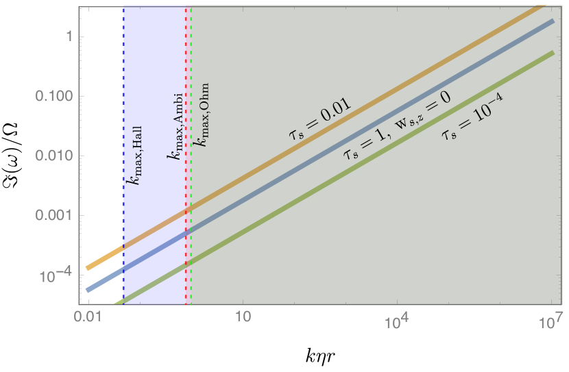
Figure 7: The ideal magnetosonic RDI (dust-gas instabilities resonant with slow-magnetosonic waves; here neglecting rotation or stratification effects), for $\beta=100$ and grain sizes as labeled (blue solid line, $\tau_{s}=1$; orange solid line, $\tau_{s}=0.01$; green solid line, $\tau_{s}=10^{-4}$. We use parameters appropriate to the MMSN model at $r\approx 1.5\mathrm{AU}$, with $\eta=0.001$ (as above), $\mu=0.01$, and $\gamma_{\mathrm{gas}}=5/3$. Noting that the magnetic field might be primarily in the toroidal direction, we specify the angle between field and drift $\theta_{w}=80^{\circ}$, then chose the mode angles $\theta_{k}^{B}$, $\varphi_{k}^{B}$ such that the resonant condition is satisfied ($\hat{\bm{k}}\cdot{\bf w}_{s}=v_{S}$) and the growth rate is approximately maximal for this RDI (see Eq. (7.2); this is $\theta_{k}^{B}\approx 69^{\circ}$, $\theta_{k}^{B}\approx 85^{\circ}$, and $\theta_{k}^{B}\approx 89.95^{\circ}$ for $\tau_{s}=1$, $\tau_{s}=0.01$, and $\tau_{s}=10^{-4}$, respectively). For the $\tau_{S}=0.01$ and $\tau_{s}=10^{-4}$ curves, we evaluate $w_{s}$ as that arising from both the NSH and vertical settling drift, while for $\tau_{s}=1$ we use only the NSH drift (i.e., $\mathrm{w}_{s,z}=0$; which makes ${w}_{s}$ a factor $\sim\eta^{1/2}$ smaller). The vertical dashed lines and shaded regions show where we expect nonideal effects to become important (see §7.2.3) due to Ohmic diffusion (green dashed line), ambipolar diffusion (red dashed line), or the Hall effect (blue dashed line). We use an ionization fraction $x_{e}\sim 10^{-10}$ and the MMSN model (the gray shaded region shows where all three effects are important). For typical expected parameters of protoplanetary disks (at least near the midplane in the regions of the disk not too close to the star), the magnetosonic RDI is suppressed by nonideal effects before reaching large growth rates.

7.2.3 Nonideal MHD effects

Due to the very low ionization fraction, nonideal MHD effects play a key role in protoplanetary disks (see, e.g., Blaes & Balbus, 1994; Wardle, 1999; Balbus & Terquem, 2001; Kunz & Balbus, 2004; Wardle, 2007; Bai & Stone, 2013). In particular, $\eta_{\mathrm{Ohm}}$, $\eta_{\mathrm{Hall}}$, and $\eta_{\mathrm{Ambi}}$ in Eq. (7.1) may not be assumed small throughout the disk and can strongly influence the dynamics (Bai & Stone, 2013; Lesur et al., 2014; Bai, 2017). For the slow-magnetosonic RDI, these terms become important when $\eta_{\mathrm{Diss}}k^{2}\bm{B}\sim\partial_{t}\bm{B}\sim kv_{S}\bm{B}$ (since $\omega\sim kv_{S}$), suggesting that the maximum $k$ at which we can expect the standard magnetosonic RDI to operate is $k_{\mathrm{max,Diss}}\sim v_{S}/\eta_{\mathrm{Diss}}$, where $\eta_{\mathrm{Diss}}$ can be one of $\eta_{\mathrm{Ohm}}$, $\eta_{\mathrm{Hall}}$, or $\eta_{\mathrm{Ambi}}$. Using the notation of Lesur et al. (2014) (see also Balbus & Terquem 2001; Wardle 2007; Bai & Stone 2013), the diffusivities are,

$$\eta_{\mathrm{Ohm}}\approx\frac{c^{2}m_{e}n\langle\sigma v\rangle_{e}}{4\pi e^{2}n_{e}},\>\eta_{\mathrm{Hall}}\approx\frac{Bc}{\sqrt{4\pi}en_{e}},\>\eta_{\mathrm{Ambi}}\approx\frac{B^{2}(m_{n}+m_{i})}{\langle\sigma v\rangle_{i}m_{i}m_{n}n_{i}n},$$ (7.4)

where $m_{e}$, $m_{i}$, and $m_{n}$ are the electron, ion, and neutral effective masses, $n_{e}$, $n_{i}$, and $n_{n}$ are the electron, ion, and neutral number densities, and $\langle\sigma v\rangle_{e}$ and $\langle\sigma v\rangle_{i}$ are the electron-neutral and ion-neutral collision rates. In Fig. 7, we overplot $k_{\mathrm{max,Diss}}$ obtained from Eq. (7.4) from Ohmic and ambipolar diffusion and the Hall effect at an ionization fraction $x_{e}\sim 10^{-10}$, showing that the ideal magnetosonic RDI is affected by all three nonideal effects well before reaching interesting growth rates.

Figure 8: The Hall-MHD RDI (RDI resonant with Hall-whistler waves). The solid line and left-hand axis shows $\Im(\omega)$ of the fastest-growing mode, numerically calculated from Eqs. (3.1)–(3.5) and (7.1) including the Hall effect, with $k_{\mathrm{max,Hall}}\sim v_{A0}/\eta_{\mathrm{Hall}}=(v_{A0}t_{s0})^{-1}$. We use $\beta=100$, $\mu=0.01$, ${w}_{s}=0.1v_{A0}$, $\theta_{w}=80^{\circ}$, $\theta_{k}^{B}=86^{\circ}$, $\varphi_{k}^{B}=20^{\circ}$, and $\gamma_{\mathrm{gas}}=5/3$. Note that we use units normalized to the dust stopping time (rather than disk units), because this figure is intended as a general example and we have not embarked on a full analysis of the Hall-MHD RDIs. The right-hand axis and dashed lines show the dispersion relation $\Re(\omega)$ for Hall-MHD waves (the Alfvén, whistler, and fast branches, as labeled), while the black thin dashed line shows $\bm{k}\cdot{\bf w}_{s}$. At the resonance condition, $\bm{k}\cdot{\bf w}_{s}=\omega_{\mathrm{whist}}$ (vertical dotted line), $\Im(\omega)$ peaks strongly—the Hall-whistler RDI. Similarly, the Hall-Alfvén RDI occurs in resonance with the Alfvén branch, although it has somewhat lower growth rates.

A secondary question then becomes: are there different, nonideal MHD RDIs, which can operate for $k>k_{\mathrm{max,Diss}}$? For an RDI to be generically unstable when ${w}_{s}\ll c_{s}$, the fluid must support some undamped wave with similar characteristics to the slow mode (in particular a phase velocity that approaches zero at some angle). Unfortunately, this immediately rules out an RDI modified by Ohmic diffusion, since for constant $\eta_{\mathrm{Ohm}}$, the relevant term in Eq. (7.1) is simply $\eta_{\mathrm{Ohm}}\nabla^{2}\bm{B}$, which damps all $\bm{B}$ perturbations. Similarly, ambipolar diffusion, although more complicated than standard Ohmic diffusion, does not allow for any undamped or weakly damped waves other then the fast wave, in the regime of interest. However, the Hall term, $\nabla\times(\eta_{\mathrm{Hall}}\bm{J}\times\hat{\bm{b}})$, does not dissipate waves, but simply acts to modify the slow and shear-Alfvén waves into whistler and Alfvén branches. These no longer have a constant phase velocity for $k>k_{\mathrm{max,Hall}}$ ($\omega_{\mathrm{whist}}\sim k^{2}$ for the whistler branch; $\omega_{\mathrm{Alfv}}\sim\mathrm{const.}$ for the Alfvén branch; see Fig. 8), but can still cause a “Hall-whistler RDI” or “Hall-Alfvén RDI” at the wavenumbers for which $\bm{k}\cdot{\bf w}_{s}=\omega_{\mathrm{whist}}$ or $\bm{k}\cdot{\bf w}_{s}=\omega_{\mathrm{Alfv}}$ respectively. This provides an entertaining example of the RDI in a system with a more complex wave structure, and so in Fig. 8 we show a numerical calculation of the Hall-whistler RDI growth rate, along with the dispersion relation of Hall-MHD waves. We see that, exactly as predicted in §4, $\Im(\omega)$ peaks strongly when $\bm{k}\cdot{\bf w}_{s}=\omega_{\mathrm{whist}}$. However, even when the Hall terms dominate, ambipolar and Ohmic diffusion terms are generally still important at relatively low $k$ (see Fig. 7), and will damp the Hall-MHD RDIs. For this reason we do not expect the Hall-MHD RDIs to be of particular importance in protoplanetary disks, at least under typical disk midplane conditions at radii $r\gtrsim 0.1\rightarrow 1\,\mathrm{AU}$ (where a MMSN-type model applies). However, it is worth noting that ideal MHD can be a reasonable approximation in both the upper regions (well above the midplane; see, e.g., Bai, 2017) and inner regions (close to the central protostar; see, e.g., Flock et al., 2017) of the disk, which are thought to be well ionized. While the physics is such regions can also become more complex due to the expected higher levels of turbulence (the magnetorotational instability is likely to be unstable), and dust sublimation, it is worth noting that the magnetosonic RDI may become much more relevant under these more extreme conditions. This is discussed further below (§9.4).

8 Physical effects not included in our analysis

There are a variety of physical effects not included in the derivations and discussions above. While the complexity of disk and dust models can be increased, nearly without bound, by including grain and fluid chemistry (e.g., Bai & Goodman, 2009), nonideal magnetic effects (see §7.2.3), grain charging, and radiation effects, it is beyond the scope of this work to consider these in any serious detail. Here we simply examine some simple effects that we have neglected in our model, Eqs. (3.1)–(3.5), and offer some commentary on how these might affect the various RDIs studied in §§5–7. Throughout this section, to obtain simple order-of-magnitude estimates, we shall use the standard MMSN values for disk parameters from Chiang & Youdin (2010), with a dust grain of density $\bar{\rho}_{d}\approx 1\,\mathrm{g}\,\mathrm{cm}^{-3}$.

Viscosity

The viscosity of the gas damps small-scale motions and becomes important (i.e., damps the RDI) when $\omega\,\delta u\sim\nu_{\mathrm{vis}}k^{2}\delta u$, where $\delta u$ is the velocity perturbation and $\nu_{\mathrm{vis}}$ is the kinematic viscosity. Using $\nu_{\mathrm{vis}}\sim c_{s}\lambda_{\mathrm{mfp}}$, we find the maximum RDI wavenumber (where viscosity is not important), $k_{\mathrm{max}}\sim\omega^{1/2}(c_{s}\lambda_{\mathrm{mfp}})^{-1/2}$, or using the MMSN model,

$$k_{\mathrm{max}}\eta r\sim 3\times 10^{4}\left(\frac{\omega}{\Omega}\right)^{1/2}\left(\frac{r}{\mathrm{AU}}\right)^{-13/28},$$ (8.1)

where $\omega$ here includes both the real and imaginary parts.

Dust separation

The fluid approximation used to model the dust is valid only for scales larger than the separation between individual grains. This is simply $\lambda^{\mathrm{dust}}_{\mathrm{sep}}\sim n_{d}^{-1/3}$, or $k_{\mathrm{max,sep}}\eta r\sim(2\pi/\lambda^{\mathrm{dust}}_{\mathrm{sep}})\eta r\sim 10^{7}(r/\mathrm{AU})^{9/14}(\mu/0.01)^{1/3}(R_{d}/\mathrm{cm})^{-1}$. Alternatively, in terms of the stopping time, one finds, $k_{\mathrm{max,sep}}\eta r\sim 10^{4}(r/\mathrm{AU})^{15/7}(\mu/0.01)^{1/3}\tau_{s}^{-1}$ for grains in the Epstein regime and $k_{\mathrm{max,sep}}\eta r\sim 4\times 10^{5}(\mu/0.01)^{1/3}\tau_{s}^{-1/2}$ for grains in the Stokes regime. For most regimes of interest (e.g., at small $\tau_{s}$), these scales are smaller than the viscous cutoff, Eq. (8.1).

Background turbulence

If, on some scale $k$, the turnover time of an eddy is faster than the growth rate of the RDI, we cannot treat the background as in equilibrium over this timescale. The actual effects of turbulence in this limit are unclear—while it is commonly treated as a diffusive process, numerous studies have shown that it can drive very strong grain concentration on small scales (Bracco et al., 1999; Cuzzi et al., 2001; Pan et al., 2011; Hopkins, 2016a). A commonly used model for turbulence in disks (Shakura & Sunyaev, 1973) is to assume that the accretion is caused primarily by the turbulent stress, and that the level of turbulence is $u^{2}\sim\alpha c_{s}^{2}$ (where $u$ here is the rms turbulent velocity at the outer scale). A very simplistic estimate of $u_{k}$, the strength of the turbulent velocity field on scale $k$, then comes from assuming a Kolmogorov cascade (Kolmogorov, 1941) with outer scale turnover time $t_{\mathrm{eddy,outer}}\sim\Omega^{-1}$. This leads to $u_{k}\sim\alpha^{1/3}c_{s}^{2/3}\Omega^{1/3}k^{-1/3}$ (the outer scale of the turbulence is $k_{\mathrm{outer}}\sim\alpha^{-1/2}\Omega/c_{s}$), and suggests that the RDI can grow so long as $\Im[\omega(k)]\gtrsim t_{\mathrm{eddy}}^{-1}\sim\alpha^{1/3}c_{s}^{2/3}\Omega^{1/3}k^{2/3}$. However, this picture of turbulent accretion in protoplanetary disks has recently been called into question by both observations (Flaherty et al., 2015; Teague et al., 2016; Flaherty et al., 2017) and theory (e.g., Gammie, 1996; Gressel et al., 2011; Lesur et al., 2014; Simon et al., 2015; Bai, 2017). In particular, the turbulence throughout much of the disk may be much weaker than inferred from accretion rates, because the angular momentum transport necessary for accretion can instead be caused by winds. Given this, it may in fact be more appropriate to estimate instability properties assuming a laminar disk profile.

Grain charge

We have neglected the influence of grain charging, which can be important, both to grain dynamics and the chemistry of the disk, especially for smaller grains (Ilgner & Nelson, 2006; Okuzumi, 2009; Ilgner, 2012). A simple estimate for when grain charging becomes important to dust dynamics is when the influence of magnetic fields on the grain is greater than that of the neutral drag, viz., when $t_{L}=m_{d}c/(|q_{d}|B)\lesssim t_{s}$, where $t_{L}$ is the Larmor time, and $m_{d}$ and $q_{d}=Ze$ are the dust mass and charge. Translating this condition into $\tau_{s}$ and the MMSN model, one finds that grains of size $\tau_{s}\lesssim 2\times 10^{-11}(r/\mathrm{AU})^{2.2}\beta^{-1/4}|Z|^{1/2}$ (where $\beta=8\pi p_{0}/B^{2}$) will be directly affected by magnetic fields (this expression is for grains in the Epstein regime, charge is effectively never important for grains in the Stokes regime). We note that although grain charge can become very large, perhaps up to $Z\sim-10^{5}$ (Okuzumi, 2009), this only occurs for larger grains (large $\tau_{s}$), so it is not likely that this effect will be important in disks. However in more rarefied regions (e.g. disk winds) the effects could be important. Similarly, charged grains experience electrostatic interactions (Coulomb drag, as well as photo-electric and photo-desorptive interactions in the presence of hard radiation sources) with the gas. However as noted in Lee et al. (2017) (see also Draine & Salpeter 1979), Coulomb drag only dominates Epstein/Stokes drag when the ionization fractions in the gas exceed $x_{e}\gtrsim 0.03$, vastly larger than expected in protoplanetary disks.

Grain-grain collisions

We have neglected any influence from grain-grain collisions, which would act to thermalize the grains and invalidate our assumption that they behave as a pressureless fluid (Jacquet et al., 2011; Johansen et al., 2012). This is a reasonable approximation considering that we have focused on the low metallicity limit ($\mu\ll 1$) throughout this work (except App. A). Of course, collisions could become important in the non-linear evolution of the RDIs here, as they produce strong local dust clumping.

9 Application to planetesimal formation

In this section, we explore some possible physical consequences of the instabilities discussed in §§5–7. In particular, we consider physical scenarios where the RDIs discussed above may be important, organizing the discussion around the instability type (i.e., epicyclic, BV, or magnetic), in a similar way to §§5–7.

9.1 The YG streaming instability

The primary contribution of this work to the theory of the Youdin-Goodman (YG) streaming instability, which is applicable to dust streaming in the midplane of the disk, has been to give simple analytic expressions for the YG streaming instability’s growth rate and fastest-growing wavenumbers (e.g., Eq. (5.10)). To our knowledge, these have not appeared in previous works, but may be useful for simple estimates and/or numerical tests.

In addition, we have provided a simple interpretation for why the instability exists: it arises due to the resonance between the dust drift velocity ${\bf w}_{s}$ and the gas epicyclic modes in the disk, which propagate with phase velocity $V_{\mathrm{epi}}=\pm{\bm{k}}\cdot\bm{\Omega}/k^{2}$. In the frame of the drifting dust, the epicyclic wave is stationary. As described in the simple model of Fig. 1, the wave’s pressure perturbations attract the dust, and the dust feedback acts to further enhance the magnitude of the pressure perturbations—a feedback that results in instability. It is therefore the “epicyclic RDI.” We reiterate that this interpretation is not in conflict with previous interpretations of the mechanism for the YG streaming instability (Youdin & Goodman, 2005; Youdin & Johansen, 2007; Jacquet et al., 2011)—indeed, it is through its interaction with the epicyclic wave that the dust is attracted to pressure maxima. Rather, the interpretation provides a clear prediction of the fastest-growing wavenumbers ($\bm{k}\cdot{\bf w}_{s}=\hat{\bm{k}}\cdot\bm{\Omega}$), the specific reason that the instability relies on the rotational support of the gas (this allows the gas to support epicyclic oscillations), and a clear method for extending the analysis to more complex physical situations.

We have also shown (App. A) that the fastest-growing mode with horizontal dust streaming when $\mu>1$ (dust dominates gas by mass), is not technically the same mode as the YG streaming instability at $\mu<1$ (the epicyclic RDI), even though both are commonly named the streaming instability. While the epicyclic RDI does exist at $\mu>1$ (or more precisely its continuation, which involves similar physics), it is no longer the fastest-growing mode: a different mode appears which is unstable only for $\mu>1$, and has a higher maximum growth rate. The maximum growth rate of this mode increases with decreasing $\tau_{s}$ at modest $\tau_{s}$ (see Fig. 9), but it operates only at very short wavelengths when $\tau_{s}\ll 1$. We again provide simple analytic expressions for the growth rate and fastest-growing wavenumbers of this instability. We also show that it is not an RDI, but arises from joint epicyclic oscillations of dust and gas that resemble a destabilized harmonic oscillator, with the dust driving the gas and destabilizing such oscillations when $\mu>1$.

9.2 The disk “Settling Instability”

9.2.1 Basic predictions: Rapid instability growth during dust settling

Perhaps the most interesting result of this work has been the discovery of a new version of the streaming instability—the disk “settling instability”—which arises when the dust motion is dominated by its vertical settling towards the disk midplane, $\mathrm{w}_{s,z}\sim\tau_{s}c_{s}$. Most interestingly, unlike the YG streaming instability, this instability does not depend significantly on grain size. For most mode angles, the settling instability has growth rate $\Im(\omega)/\Omega\approx\mu^{1/2}\hat{k}_{x}$ around wavenumber $k\eta r\sim\eta^{1/2}/\tau_{s}$, where $\eta\sim 10^{-3}$ parameterizes the gas pressure support (see Eq. (3.8)). (These estimates depend modestly on the stratification profile and we shall consider an approximately neutrally buoyant fluid here and below for simplicity; see §6.3.5). This means that, for small grains in particular, the growth rates can be orders-of-magnitude faster than the YG streaming instability—comparable, in fact, to the disk orbital time. Moreover, the characteristic wavelengths are larger than the YG streaming instability by a factor $\sim\!\eta^{-1/2}\!\sim\!30$. Thus, a larger volume of grains can be concentrated into the structures produced by the instability, suggesting the concentrations could be more likely to be gravitationally unstable and better able to resist destruction via turbulence.

Even more surprising, at a particular “double-resonant” mode angle $\theta_{\mathrm{res}}$, where $\hat{\bm{k}}\cdot{\bf w}_{s}=0$, $\Im(\omega)$ formally increases without bound as $\Im(\omega)/\Omega\sim(\tau_{s}\,\mu\,k_{x}\eta r)^{1/3}$, once $\Im(\omega)$ is larger than $\omega_{\mathrm{EBV}}=(\hat{k}_{z}^{2}\Omega^{2}+\hat{k}_{x}^{2}N_{\mathrm{BV}}^{2})^{1/2}$. We shall consider this double-resonant mode separately in estimates below, although it appears in exactly the same physical set up as the standard settling instability (just at smaller scales). Here $\omega_{\mathrm{EBV}}$ is the frequency of joint epicyclic-buoyancy oscillations, or inertia-gravity waves, which is the natural oscillation frequency in stratified regions of the gas ($N_{\mathrm{BV}}$ is the Brunt-Väisälä frequency; see Eq. (6.14) and §9.3 below).

Importantly, these growth rate estimates are easily faster than the time required for small grains to settle to the midplane of the disk, which scales as $\Omega\,t_{\mathrm{settle}}\sim(\Omega t_{s})^{-1}=\tau_{s}^{-1}$ (for grains starting approximately one scale height above the midplane). Thus, although necessarily transient, halting once grains reach the midplane, the instability will evolve well into its nonlinear phase long before its driving force (the downwards drift) is removed. This leads us to suggest a scenario where smaller grains clump significantly, due to the settling instability, in the process of settling towards the disk midplane.

9.2.2 Potential nonlinear consequences & appearance

The settling instability modes grow fastest when $\hat{k}_{x}>\hat{k}_{z}$, so would have the appearance of concentric axisymmetric cylinders of higher dust concentration that form as the dust settles. Their fastest-growing wavelength (see Eq. (5.13)) is $2\pi/k\sim\lambda\sim\lambda_{x}\sim 2\pi\,\eta^{1/2}r\tau_{s}\sim 2\pi\,h_{g}\tau_{s}$ (this estimate can increase somewhat depending on the temperature stratification profile; see §6.3.5). This suggests that a cylinder of dust of area $A\sim 2\pi\,r\,\lambda$ (in an MMSN-type disk with with density $\Sigma\sim 2200\,{\rm g\,cm^{-2}}\,\Sigma_{\rm MMSN}\,\,(r/\mathrm{AU})^{-3/2}$; Chiang & Youdin, 2010) contains a mass of dust $M\sim 4\times 10^{24}\,{\rm g}\,(\tau_{s}/0.001)\,(\mu/0.01)\,\Sigma_{\rm MMSN}\,(r/\mathrm{AU})^{11/14}$, or enough mass to form a planetesimal of size $R_{\mathrm{plan}}\sim 1000\,{\rm km}\,(\tau_{s}/0.001)^{1/3}\,(\mu/0.01)^{1/3}\,\Sigma_{\rm MMSN}^{1/3}\,(r/\mathrm{AU})^{-0.26}\,\bar{\rho}_{\mathrm{solid}}^{-1/3}$ (here $\bar{\rho}_{\mathrm{solid}}$ is the mass density of the planetesimal in ${\rm g\,cm^{-3}}$).

While of course we cannot simply extrapolate from the linear behavior of the settling instability to directly form a planetesimal (given the very large nonlinear concentration of grains that would be necessary), this estimate does show that the overdensities it creates contain a significant amount of mass. Thus, some possible outcomes could include: (i) direct planetesimal formation as grains sediment vertically; (ii) the creation of dust clumps that later act as high-metallicity ($\mu\gtrsim 1$) seeds for the YG streaming instability in the disk midplane (which operates on smaller scales, see App. A); or (iii) the generation of alternating over-dense and under-dense rings as the dust settles, which could, given sufficiently strong dust concentration, act as “pressure bumps” in the midplane and so potentially trap even more dust (thus continuing to grow in density contrast).

Noting that simulations have found a strong dependence of the efficiency of planetesimal formation on metallicity, with a cutoff metallicity of $\mu\approx 0.02$ for $\tau_{s}\gtrsim 0.1$ grains (Johansen et al., 2009; Bai & Stone, 2010), even if the local enhancement of the metallicity were only a factor of several, it might strongly influence the planetesimal formation process. Further, small grains—which seem to require a higher local metallicity to form planetesimals (according to numerical simulations; Carrera et al., 2015; Yang et al., 2016)—may also be more efficiently clumped by the settling instability because of their longer settling times, thus reaching higher local metallicities. Such clumping may also increase the collision rate of grains (presumably proportionally to the relative density increase in the clumps), perhaps enhancing grain coagulation rates to the point where a significant population of larger grains could form at relatively low metallicities ($\mu\ll 1$) before the solids settle completely in the midplane of the disk (Dra̧żkowska et al., 2013; Dra̧żkowska & Dullemond, 2014).

Interestingly, if we speculate that some constant fraction of the dust mass concentrated in an annulus by the initial settling instability eventually ends up in a planet, and that the maximum grain size is constant in terms of $\tau_{s}$ (as models of grain-growth suggest; Birnstiel et al. 2012; Dra̧żkowska et al. 2014), then our estimates above imply the resulting object size would depend very weakly on location in the disk, as $R_{\mathrm{plan}}\propto r^{0.26}$ (or $R_{\mathrm{plan}}\propto P^{0.17}$, in terms of the orbital period $P$). This could conceivably provide a partial explanation for the observed tendency of planet sizes to vary weakly within the same disk (Weiss et al., 2017; Millholland et al., 2017).

9.2.3 Range of grain sizes where growth is rapid

Of course, simulations will be required to assess the scenarios discussed in the previous paragraphs in detail. Nonetheless, let us consider the relevant timescales more quantitatively, starting with the standard (RDI) settling instability and then considering modes at the double-resonant angle $\hat{\bm{k}}\cdot{\bf w}_{s}=0$ (these modes have higher growth rates, but smaller scales). When $\hat{k}_{x}\gtrsim\hat{k}_{z}$, the settling instability has growth rate $\Im(\omega)/\Omega\approx\mu^{1/2}\approx 0.1(\mu/0.01)^{1/2}$ at $k\eta r\sim\eta^{1/2}/\tau_{s}\approx 0.03(r/\mathrm{AU})^{2/7}\tau_{s}^{-1}\sim(h_{g}\tau_{s})^{-1}$, and thus is not affected by viscosity for $\tau_{s}\gtrsim 10^{-6}\,(r/\mathrm{AU})^{3/4}$, or $R_{d}\gtrsim 8\,(r/\mathrm{AU})^{-3/4}\,\mu\mathrm{m}$. So long as the disk is sufficiently quiescent over the growth time scales (see below), this mode grows sufficiently fast to clump the dust before it reaches the disk midplane for grains of size $\tau_{s}\lesssim 0.1\,(\mu/0.01)^{1/2}$. As discussed above, the mass contained in a single ring the size of this mode is sufficient to form a $\mathrm{km}$-sized planetesimal for effectively any grain size ($\tau_{s}\gtrsim 10^{-12}$ at $\sim\!1\mathrm{AU}$).

The double-resonant mode can grow much faster than the standard (RDI) settling instability, but is also active on smaller scales and so does not contain as much mass. We can estimate its maximum growth rate from Eq. (8.1) for the smallest scales allowed due to gas viscosity. This shows that $(\omega/\Omega)_{\mathrm{max}}\sim 12\,(\mu/0.01)^{2/5}\tau_{s}^{2/5}(r/\mathrm{AU})^{-0.2}$, so long as this value is larger than the gas epicyclic-Brunt-Väisälä frequency $\omega_{\mathrm{EBV}}\sim\Omega$ (at one scale height, depending on the temperature stratification). This suggests that grains with $\tau_{s}\gtrsim 10^{-3}$ are unstable to the double-resonant mode on small scales, with a growth rate $\Im(\omega)>\Omega$; i.e., the instability grows faster than the disk dynamical time (recall from above that grains with $\tau_{s}\gtrsim 10^{-5}$ have maximum $\Im(\omega)\sim 0.1\Omega$). This is sufficiently large to clump grains with $\tau_{s}\lesssim 1$ before they settle into the midplane, implying that effectively all grain sizes are unstable to instabilities that grow more rapidly than their vertical settling time. This rapid clumping on small scales could significantly modify grain coagulation or other properties of the dusty gas.

9.2.4 The role of turbulence

Of course, the caveat about the quiescence of the gas is an important one. The effect of turbulence in protoplanetary disks is rather difficult to estimate and quite poorly understood at the present time, but there is now significant evidence from observations (Flaherty et al., 2015; Pinte et al., 2016; Teague et al., 2016) and theory (Bai & Stone, 2013; Bai, 2017) that turbulence is quite weak in most regions of the disk. For example, the observations of Flaherty et al. (2015) place an upper limit on the turbulence level around the young star HD 163296 of $u_{\mathrm{rms}}\lesssim 0.03c_{s}$, which is significantly lower than would be inferred from the accretion rate (if accretion proceeded primarily through turbulent stresses). Instead, it has been argued recently that accretion is driven primarily by winds, with a largely laminar profile in the bulk disk (see, e.g., Bai 2017 for comprehensive simulations of protoplanetary disk accretion physics, which show a mostly laminar disk profile).

Despite this uncertainty, assuming some turbulence exists in the disk, the disk settling instability is likely to be less sensitive to the presence of turbulent motions than the standard YG streaming instability. This is for two reasons: (1) the growth rates for small grains are much faster, and (2) the characteristic wavelengths are larger.

If we parameterize the level of turbulence using $\alpha$ (which is likely to be overly pessimistic) and balance the RDI growth rate and eddy turnover time (as discussed in §8), we estimate that turbulence would likely influence the settling instability when $\tau_{s}\lesssim(0.003\rightarrow 0.03)\,(\alpha/10^{-4})^{1/2}\,(\mu/0.1)^{-3/4}$ (where the range depends on assumptions about the largest eddy turnover times in units of $\Omega^{-1}$, and the width of the resonance). A similar estimate argues that turbulence is important for the YG streaming instability when $\tau_{s}\lesssim(0.1\rightarrow 1)\,(\alpha/10^{-4})^{1/5}\,(r/\mathrm{AU})^{4/35}\,(\mu/0.1)^{-3/10}$. In other words, compared to the YG streaming instability, the settling instability is likely to be less affected by external turbulence and survive for smaller grain sizes. For lower levels of turbulence, the settling instability becomes even more robust compared to the YG streaming instability (the scaling with $\alpha$ is different), while the opposite occurs at lower $\mu$. The double-resonant mode can be influenced by turbulence for effectively all grain sizes, because its growth rate increases (in a homogeneous background) without limit with $k$ as $\sim k^{1/3}$: in a Kolmogorov-type cascade, this suggests there will be some sufficiently high $k$ where eddy turnover times ($\sim k^{-2/3}$) become shorter than the mode growth timescales.

We also note that dust-induced turbulence caused by the extra mass loading in the midplane is likely only relevant in a thin layer near the midplane (Garaud & Lin, 2004; Takeuchi et al., 2012), and thus presumably more important for the YG streaming instability than the settling instability. In contrast, some other turbulence-generation mechanisms, such as shear or buoyancy induced instability (Nelson et al., 2013; Klahr & Hubbard, 2014; Flock et al., 2017) would presumably more strongly affect regions away from the disk midplane. Ultimately, any useful turbulence-related constraints on grain concentration due to the disk settling instability will require nonlinear simulations and better theoretical understanding of disk accretion mechanisms and instabilities. Given the potential importance of global effects, disk thermodynamics, and other complicated nonideal effects, this is a rather difficult computational problem to tackle in detail.

9.2.5 Robustness of the Settling Instability

The fundamental character of the settling instability (vertical-epicyclic RDI) is robust to a wide range of assumptions or details of our derivation, including: (1) vertical or radial stratification of the disk (assuming $kh_{g}\gg 1$); (2) gas compressibility; (3) the form of the drag law (Epstein or Stokes drag); (4) the gas equation-of-state; (5) including or ignoring radial or azimuthal streaming velocities (in the dust or gas); (6) including or ignoring gas streaming motion; (7) external magnetic forces (ideal or non-ideal MHD in the gas, and Lorentz forces on the dust, so long as the Lorentz forces are sub-dominant to drag); (8) changing the gravitational potential (from Keplerian), which simply modifies the epicyclic frequency by an order-unity constant; and (9) self-gravity (at least for linear perturbations assuming the disk initially has $Q\gg 1$). Note that we have explicitly verified all of these properties, but did not show several in detail precisely because they have no significant effect in the relevant limits. As discussed above, the settling instability is also unstable for any finite dust-to-gas ratio $\mu$ and grain size/stopping time $\tau_{s}$. The relevant question, as discussed above, is whether or not the instability grows fast enough to generate interesting nonlinear behavior before grains settle into the disk midplane (or before structures are disrupted by external turbulence).

9.2.6 The Settling Instability in simulations

A question that naturally arises is whether the disk settling instability has been observed in previous simulations. So far as we are aware, it has not, for two likely reasons: first, it has been common (e.g., Bai & Stone 2010) to simulate only a small portion of the disk plane, so as to capture more accurately the concentration of dust at the disk midplane; second, most works have focused on larger grain sizes. Both of these choices decrease the settling time of dust (or eliminate settling entirely), and it seems that this has been too short to see the instability develop in previous simulation work. Let us consider Yang et al. (2016) in more detail, which, to our knowledge, has been the closest to resolving the vertical streaming instability, due their small particles and high-resolution two-dimensional domains. Their highest resolution simulation, with $5120$ grid cells per $h_{g}$ and $\tau_{s}=0.01$, can resolve scales up to $k\eta r\sim 160$, suggesting the growth rate of the double-resonant mode at the smallest scales is $\Im(\omega)/\Omega\approx 0.3$. However, their simulation initializes grains at a height of $h_{d,\mathrm{init}}\sim 0.02h_{g}$ (barely above the midplane), which suggests that they settle to the midplane within $t\sim 2\Omega^{-1}$, and there is simply not enough time for grains to clump significantly due to either the settling instability or the double-resonant mode. Similarly, while the study of Yang & Johansen (2014) uses domains of large vertical extent and an initially uniform dust density distribution in $z$, their rather large particles ($\tau_{s}\approx 0.3$) again cause the particles to settle quickly, and the resolution is too low ($160$ cells per $h_{g}$ for the largest domains) to see the fast-growing double-resonant mode. Nonetheless, it seems quite feasible to study this mode in simulation, at least in two dimensions, potentially using a setup similar to Yang et al. (2016), or to Lambrechts et al. (2016) but with rotation included (see §9.3.1).

9.3 Brunt-Väisälä RDI

As a subsidiary result of this work, we analyzed the Brunt-Väisälä (BV) RDI, which arises as a result of the resonance between streaming dust and BV oscillations in a stratified fluid. In essence, the instability is relatively simple: the streaming dust sees a stationary BV oscillation, which involves motions of the gas that advect the background density/entropy gradient, and a small pressure perturbation. The dust can interact with gas density perturbations through the dependence of the stopping time $t_{s}$ on the gas density; this enables the alternate RDI mechanism discussed in §1.2 and is parameterized through the $\zeta_{\rho}\Lambda_{S}$ term in Eq. (6.11). Dust is also drawn into pressure maxima, which, as shown in Fig. 1, helps to destabilize the mode (note that there remain theoretical uncertainties regarding the exact form of this term; see §6.1.1). When the dust-gas drift is dominated by the dust settling in the direction of gravity, the mode’s growth rate is

$$\Im(\omega)\approx\left(\frac{\mu}{2}\right)^{1/2}\hat{k}_{x}\left[L_{0}^{-1}\frac{\mathrm{w}_{s,z}}{t_{s}}\left(1+\frac{\Lambda_{S}}{2}\right)\right]^{1/2},$$ (9.1)

for grains in the Epstein drag regime. It grows at the scale where $\bm{k}\cdot{\bf w}_{s}$ matches the Brunt-Väisälä frequency, or at $(kL_{0})^{-1}\sim\lambda/L_{0}\sim{w}_{s}/c_{s}$. Here $L_{0}^{-1}=\gamma_{\mathrm{gas}}^{-1}\nabla\ln P$, $\Lambda_{S}$ parameterizes the entropy/temperature stratification (see Eq. (6.1)), and $(L_{0}^{-1}\mathrm{w}_{s,z}/t_{s})^{1/2}\approx(\mathrm{w}_{s,z}/c_{s})\,t_{s}^{-1}\sim c_{s}L_{0}^{-1}$ for grains that are passively settling through the gas (i.e., when there are no external forces on grains other than gravity). The instability is likely only weakly modified by dust stratification, so long as the dust stratification is similar to, or less than, the gas stratification (see App. B).

As can be seen through analysis of the RDI including both rotation and stratification (§6.3), in disks, this BV RDI is of minor relevance compared to the epicyclic RDI, usually increasing growth rates by $\mathcal{O}(1)$ factors without changing its qualitative behavior (some of these effects were mentioned briefly above in the qualitative discussion of §9.2.1). Nonetheless, the BV RDI can occur whenever grains settle through a stratified atmosphere (with or without rotation). We can estimate when the instability could be important for dust clumping by asserting that the growth timescale timescale be shorter than the time for the particles to move through the stratified atmosphere, which is of length $\sim\!L_{0}$. From the estimates above, this requires $\Im(\omega)\sim\mu^{1/2}t_{s}^{-1}{w}_{s}/c_{s}\gtrsim{w}_{s}/L_{0}$, which may be rearranged to $\mu^{1/2}\gtrsim{w}_{s}/c_{s}\sim t_{s}g/c_{s}\sim\lambda/L_{0}$. Thus we see that the instability becomes faster growing, compared to the settling time, for smaller grain sizes (small $t_{s}$), although it also grows on smaller scales. There may, therefore, be a variety of non-disk systems where the instability plays a critical role—for example, in the atmospheres of forming giant planets (Ikoma et al., 2000; Lambrechts et al., 2016). The BV RDI may also be observable in terrestrial experiments (Guazzelli & Hinch, 2011)

9.3.1 The Brunt-Väisälä RDI in simulations

In Lambrechts et al. (2016), the authors numerically set up a stratified pressure-supported gaseous atmosphere and allowed grains to settle in the direction of gravity, observing significant clumping of the grains as they settled. Using the parameters of their fiducial setup (their run2 or run3), we estimate that the BV RDI in their setup should have a growth rate of approximately $\Im(\omega)\,t_{s}\approx 0.08\,\mu^{1/2}\hat{k}_{x}$ at wavenumber $gt_{s}^{2}k\approx 0.08\,\hat{k}_{x}/\hat{k}_{z}$ (we use the “friction units” of Lambrechts et al. 2016 here, with $z$ the direction of stratification). This suggests that the BV RDI is unstable for in their simulations for oblique wavenumbers ($\hat{k}_{x}>\hat{k}_{z}$). Indeed, their measured growth rates in their lower-$\mu$ runs (runs1.01–runs4.01), where our analytic expressions are most accurate, agree within a factor of several with our BV-RDI predictions and scale as $\Im(\omega)\sim\mu^{1/2}$ as we predict (see Lambrechts et al. 2016, Figure 10). This interpretation is also commensurate with the toy model put forth by Lambrechts et al. (2016), which invoked the importance of buoyancy for the instability. However, the instability was not found in their linear stability analysis (their Appendix A) due to the neglect of stratification of the gas in that analysis, which is crucial to the BV RDI (including compressibility could also have led to different instabilities in their analysis, see HS17).

9.4 Magnetic RDIs

Our final, albeit brief, exploration of RDIs in protoplanetary disks in this work concerned RDIs that result from resonances with magnetic waves. In principle, such instabilities could grow rapidly in a well-ionized gas on small scales, for dust-gas drift velocities comparable to those in protoplanetary disks. However, we found that the significant non-ideal effects, which arise due to the low ionization fraction in the bulk regions of stellar disks, will likely tend to damp out any such RDIs at scales well below where their growth rates become astrophysically interesting (see Fig. 7). While MHD with one such non-ideal effect, the Hall effect, can support a number of RDIs because it has undamped waves (the Hall-whistler and Hall-Alfvén RDIs, see Fig. 8), both Ohmic and Ambipolar diffusion act to damp such instabilities, and thus magnetic instabilities are unlikely to be of interest under standard midplane disk conditions (i.e., those in the bulk of the disk in the MMSN model). Magnetic RDIs may, however, be more important in the inner regions of the disk, or in the outer layers, where the proximity to the protostar suggests the gas/plasma is likely well approximated by ideal MHD (see, e.g., Flock et al. 2017). Depending on the levels of turbulence in such regions, the slow magnetosonic RDI could act to clump grains on small scales, including those grains with dynamically important charge (Hopkins & Squire, 2018).

Another place where the magnetosonic and acoustic RDIs may be relevant is in disk winds, which are now thought to be a key accretion mechanism in protoplanetary disks (see, e.g., Bai & Stone 2013; Simon et al. 2015; Bai 2017). Such winds can reach supersonic velocities and are likely well ionized (Bai et al., 2016). Thus, if a wind contained dust, it could be unstable to both the slow and the fast magnetosonic RDIs (or the related acoustic RDI). This would cause dust clumping over quite short timescales (see HS17), potentially modifying important properties of the dust-laden gas, e.g., its opacity. One can estimate a critical grain size that is swept up by a wind (or by gas evaporation) by balancing the downwards force due to gravity against the drag from the wind (see Gorti et al. 2015). For a wind launched with a velocity $\sim c_{s}$ from a scale height $z\sim 4h_{g}$, this suggests particles with $R_{d}\lesssim 6(r/\mathrm{AU})^{-3/2}\mathrm{cm}$ can be swept up by the wind, if they exist at this scale height. As they are swept up and accelerated by the gas, the particles reach the gas velocity after $t\sim t_{s}$, implying that the RDI must have $\Im(\omega)\gtrsim t_{s}^{-1}$ for the instability to have time to develop. Noting that the growth rate of both the hydrodynamic and magnetic RDIs scale as $\Im(\omega)t_{s}\sim\mu^{1/2}(k\,c_{s}\,t_{s})^{1/2}$ when ${w}_{s}\gtrsim c_{s}$, we see that modes with $k\eta r\gtrsim 3(R_{d}/\mathrm{cm})^{-1}(T_{\mathrm{wind}}/1000\mathrm{K})^{-1}(\mu/0.01)^{-1}$ grow sufficiently fast to clump the dust (where $T_{\mathrm{wind}}$ is the temperature of the wind). Of course, because all of the larger grains and most of the smaller grains will have sedimented towards the midplane, the dust-to-gas ratio $\mu$ at the wind launch point may be very low (Gorti et al., 2015).

10 Conclusion

In this work, we have introduced and studied a variety of well-known and new instabilities of streaming dust, exploring their relevance to planetesimal formation in protoplanetary disks. Each of these instabilities is related to the well-studied “streaming instability” (Youdin & Goodman, 2005) through the recognition that they are all—including the streaming instability—members of the broad class of Resonant Drag Instabilities (RDIs; see SH17 and HS17). In a dust-gas mixture where there is a nonzero relative velocity ${\bf w}_{s}$ between the two phases, an RDI occurs at wavenumber $\bm{k}$ whenever the dust streaming frequency, $\bm{k}\cdot{\bf w}_{s}$, resonates with (equals) the frequency $\omega_{\mathcal{F}}$ of an undamped wave in the gas. In the frame of the drifting dust grains, a resonant wave is stationary and attracts dust towards its pressure maxima. The backreaction of the dust on the gas then acts as a force towards these same pressure maxima, enhancing them further and promoting exponential growth of the perturbation (see Fig. 1). At low metallicities, RDI modes, with $\bm{k}\cdot{\bf w}_{s}=\omega_{\mathcal{F}}$, are always the fastest-growing drag-induced instabilities in the system (SH17). Further, they always act to concentrate grains as the instability grows.

This RDI theory described above suggests a general algorithm for discovering new dust-gas streaming instabilities: (i) chose an undamped gas wave, which oscillates with some frequency $\omega_{\mathcal{F}}$; (ii) compute the resonant wavenumbers $\bm{k}_{\mathrm{res}}$ for which $\bm{k}\cdot{\bf w}_{s}=\omega_{\mathcal{F}}$; (iii) use the RDI formula, Eq. (4.3), to compute the growth rate of the fastest-growing modes in the system, which occur at wavenumber $\bm{k}=\bm{k}_{\mathrm{res}}$. The results of this paper have simply been an application of this algorithm to some different oscillation modes of disks. Remarkably, we have shown this leads to several new instabilities, which (to our knowledge) have not been previously recognized. For smaller dust grains, these can have growth rates that are orders-of-magnitude faster than the Youdin & Goodman (2005) streaming instability. An aspect of this result that deserves emphasis is that even the smallest grains are subject to fast-growing RDIs, suggesting that a separate treatment of dust and gas dynamics may be important for many applications.

10.1 Relation to known instabilities

One purpose of this work has been to interpret the standard (YG) streaming instability within the RDI framework, give simple analytic expressions for its growth rates and fastest-growing wavenumbers, and put forward a heuristic toy model for its operation (§1.2). The high-metallicity $\mu>1$ case, which we show is actually a different instability, is analyzed separately in App. A. The expressions we derive compare well against numerical solutions of the dispersion relation (e.g., Figs. 2–3), while the interpretation of the streaming instability as an RDI is helpful for gaining a general physical picture for its mechanism and extensions.

10.2 New instabilities with rapid growth rates

Going beyond the well-studied streaming instability, we have explored several different RDIs, all of which should be present in disks. Most interestingly, we have shown that when grains settle towards the midplane of the disk, a new instability—the disk settling instability—appears. Its growth rate is approximately independent of grain size ($\tau_{s}$), and for small grains, is orders of magnitude larger than the standard YG streaming instability. Moreover, the settling instability  grows on larger wavelengths (by a factor $\eta^{-1/2}\sim 30$) than the YG streaming instability, potentially allowing it to concentrate a larger mass of grains and likely making it more robust against external turbulence in the disk. We show that for a wide range of grain sizes, the growth timescales are significantly shorter than the dust’s vertical settling time, and, even at low dust-to-gas ratios, comparable to or shorter than the disk orbital period.

This suggests a picture where small grains could clump significantly in the process of settling towards the midplane of the disk, with potentially interesting consequences for grain growth and other properties (e.g., opacity). We expect the instabilities to aggregate dust into narrow radial annuli or bands as it sediments, potentially building pressure bumps and dust traps into the initial distribution of dust in the midplane, without any external processes required. If the clumping goes further during sedimentation, it could possibly nonlinearly reach sufficient densities to trigger planetesimal formation via gravitational collapse, or (more conservatively) could generate high-metallicity seeds for the standard YG streaming instability once the dust clumps reach the midplane. This suggests a mechanism that could allow planetesimal formation at lower metallicities, for smaller grain sizes, than inferred from simulations up to now (Johansen et al., 2009; Bai & Stone, 2010; Carrera et al., 2015).

We have also examined a variety of other RDIs, including those caused by a resonance with buoyancy (Brunt-Väisälä) oscillations, sound waves, and various MHD waves. While we have mostly found that these are less important than the settling instability, each has potential relevance in some regimes. For the reader interested in a quick overview of these results, we have outlined the behavior of each RDI and given astrophysically relevant estimates their properties in §9, while §2 lists each of the instabilities covered in this work.

10.3 Future work

While we have analyzed the main types of oscillations that could be expected in cooler disks around young stars, there remain a variety of interesting avenues for exploration. On the linear side, it will be interesting to explore the interaction of dust with non-axisymmetric waves, which have been completely ignored in this work (because a time-dependent or global analysis is necessary to study such modes). One interesting possibility is spiral density waves (Nelson & Papaloizou, 2004; Heinemann & Papaloizou, 2009; Pérez et al., 2016), which, due to their large gas perturbations, may interact relatively strongly with dust. We have also largely focused our analysis on MMSN-type disks, at modest distances ($\sim$ AU). Under more extreme conditions—e.g., around massive stars, or very close/far from the star—it is possible that the different gas conditions could change the relative importance of different RDIs or even produce new RDIs.

On the computational front, the path forward is clear: the role of the settling instability in planetesimal formation can only be studied in real detail using simulations of its nonlinear evolution. These are quite feasible with present-day computational resources, at least in local two-dimensional domains, and require simulating the settling of dust through a rotating stratified disk atmosphere (see §9.2.6 and §9.3.1 for further discussion of simulations). Whether the settling instability can, ultimately, have a significant effect on the planetesimal formation process will depend on the relative clumping of dust that occurs during its nonlinear evolution.

Appendix A The high-$\mu$ limit of the streaming instability

In this appendix, we study the standard YG streaming instability, with horizontal drift in the disk midplane, in the high-$\mu$ limit. Simulations show that the YG streaming instability concentrates grains to sufficient densities to form planetesimals only after they have reached high local metallicities (e.g., Johansen et al., 2009; Bai & Stone, 2010), so this limit is particularly important physically. However, as we show below, the fastest growing mode in this regime has a different character to the RDIs studied in the main text (see also, e.g., Fig. 4 of Youdin & Goodman 2005), and is in fact a separate mode that becomes unstable only once $\mu>1$. Our purpose here is to illustrate this different character of the high-$\mu$ instability, and give analytic expressions for its fastest growing wavenumber and growth rate. We do so via expansions of the the dispersion relation in $\tau_{s}\ll 1$, quantifying how the instability is confined to very short wavelengths when $\tau_{s}\ll 1$ and $\mu\gg 1$ (see also Youdin & Goodman, 2005; Youdin & Johansen, 2007).

A.1 Instability criterion and growth rates

Following Youdin & Goodman (2005), we shall treat the instability assuming incompressibility of the gas. We shall proceed by expanding the dispersion relation, which is derived from the characteristic polynomial of the linearized (unstratified) epicyclic system (Eqs. (3.1)–(3.7)), after inserting the NSH drift velocities (Eqs. (3.17)–(3.18)). Note that we do not transform into the frame of the gas here—i.e., we insert $\bm{u}=\bm{u}_{0}+\delta\bm{u}$ and $\bm{v}=\bm{v}_{0}+\delta\bm{v}$—because it makes the character of the instability more clear.

Our first step is to note that the instability grows fastest when $k_{z}\gg k_{x}$ (Youdin & Goodman, 2005; Jacquet et al., 2011), and expand the dispersion relation in $(k_{z}\eta r)^{-1}$. Noting that $k_{x}$ of the fastest-growing mode scales as $k_{x}\eta r\sim\tau_{s}^{-1}$, we then insert $k_{x}\eta r\sim\tau_{s}^{-1}$ and expand the resulting expression in $\tau_{s}$. The result (at order $\tau_{s}^{-3}$) is effectively the terminal velocity approximation of Youdin & Goodman (2005) (see their appendix), and yields the simple polynomial

$$(\mu+1)^{2}\left(\frac{\omega}{\Omega}\right)^{3}+2\tau_{s}k_{x}\eta r\,\left(\frac{\omega}{\Omega}\right)^{2}-(\mu+1)^{2}\left(\frac{\omega}{\Omega}\right)+2\,(\mu-1)\,\tau_{s}\,k_{x}\eta r=0.$$ (A.1)

While the solutions to this equation (which is identical to Eq. (39) of Youdin & Goodman (2005) with $k_{z}\approx k$), can be written in closed form if desired, they are not very enlightening. However, expanding the solutions of (A.1) to second order in $\tau_{s}k_{x}\eta r\gg 1$, two of the roots are

$$\frac{\omega}{\Omega}\approx\pm i\sqrt{\mu-1}+\frac{\mu(\mu+1)^{2}}{4\,k_{x}\eta r\,\tau_{s}}\mp\frac{i\mu(5\mu-4)(\mu+1)^{4}}{32\,(k_{x}\eta r\,\tau_{s})^{2}\sqrt{\mu-1}}+\ldots,$$ (A.2)

which shows that there is a separate root, unrelated to the low-$\mu$ RDI discussed in §5, which has growth rate $\Im(\omega)/\Omega=\sqrt{\mu-1}$ and so becomes unstable only for $\mu>1$ (when $\tau_{s}\ll 1$).

A.2 Characteristic wavenumbers

Equating the first and third terms in Eq. (A.2), we can estimate that the $\Im(\omega)/\Omega\approx\sqrt{\mu-1}$ solution is valid once $k_{x}\eta r\,\tau_{s}\gtrsim\mu^{1/2}(5\mu/2-2)^{1/2}(\mu-1)^{-1/2}(\mu+1)^{2}/4$ (for lower $k_{x}$ one must compute the full solutions to Eq. (A.1)). We can also evaluate the lowest unstable wavenumber from Eq. (A.1) by evaluating the point at which its discriminant crosses zero, which shows that this mode is stable for

$$k_{x}\eta r\,\tau_{s}<(k_{x}\eta r\,\tau_{s})_{\mathrm{cutoff}}\approx\frac{\mu}{3\sqrt{3}}+\frac{8}{9\sqrt{3}}+\mathcal{O}(\mu^{-1}).$$ (A.3)

This condition illustrates the very short wavelength nature of this mode—it requires $k\eta r\gg\mu\,\tau_{s}^{-1}$—and, given that high-$k$ modes are damped by viscosity or dust interparticle spacing (see §8), this can be rather restrictive when $\tau_{s}\ll 1$ and $\mu\gg 1$.

Figure 9: The growth rate of the “high-$\mu$ streaming instability”—the fastest growing unstable mode when $\mu>1$ and there is no vertical dust drift. We derive its properties in App. A, and show that it is a fundamentally different instability from the low-metallicity ($\mu<1$) YG streaming instability (the epicyclic RDI). The epicyclic RDI is the fastest-growing mode at $\mu<1$ (where the high-$\mu$ mode becomes stable), but (without vertical drift) it is slower-growing than this “high-$\mu$” mode (which is technically not an RDI) once $\mu>1$. We compare numerical solutions of the full dispersion relation (thick colored lines; only fastest-growing mode shown) with analytic solutions from App. A derived from asymptotic expansion, for different $\tau_{s}$ as labeled. We take $\mu=30$ and $k_{x}\approx 0.09\,k_{z}$ ($\theta_{k}=85^{\circ}$; this mode angle is close enough to $90^{\circ}$ such that the $k_{x}\gg k_{z}$ limit studied in the text applies well). Black crosses show the maximum growth rate ($\omega=i\sqrt{\mu-1}\,\Omega$) and fastest-growing wavenumber ($k_{x,\mathrm{max}}$; Eq. (A.3)) for small $\tau_{s}$, while dashed lines show the analytic approximations (Eq. (A.1) and Eq. (A.4), below/above $k_{x,\,\mathrm{max}}$).

While Eq. (A.2) (or the full solutions of Eq. (A.1)) predict that $\Im(\omega)$ asymptotes to a constant value at high $k_{x}$, this behavior is spurious due to our neglect of terms at next order in $\tau_{s}$. Indeed, carrying out the same expansion as led to Eq. (A.1) but now keeping the next-order terms in $\tau_{s}$, one finds terms of order $(k_{x}\eta r\,\tau_{s})^{3}/\tau_{s}^{2}$ (compared to terms of order $(k_{x}\eta r\,\tau_{s})/\tau_{s}^{3}$ in Eq. (A.1)), which become important when $k_{x}\eta r\gtrsim\tau_{s}^{-3/2}$. We thus expand again in large $k_{x}$, but now with $k_{x}\eta r\,\tau_{s}^{3/2}\sim 1$, finding the roots,

$$\frac{\omega}{\Omega}\approx\pm i\left[\left(\frac{4\mu(k_{x}\eta r)^{2}\tau_{s}^{3}}{(1+\mu)^{5}}\right)^{2}+\mu-1\right]^{1/2}\mp i\frac{4\mu(k_{x}\eta r)^{2}\tau_{s}^{3}}{(1+\mu)^{5}}.$$ (A.4)

This solution approaches $\omega/\Omega=\pm i\sqrt{\mu-1}$ for small $k_{x}\eta r$—i.e., the opposite limit to Eq. (A.2)—and there is a sharp decrease towards $\omega=0$ once $(k_{x}\eta r)^{2}\tau_{s}^{3}\gtrsim\mu^{-1}(\mu-1)^{1/2}(\mu+1)^{5}/4$. The fastest growing wavenumber of the full solution, which we term $k_{x,\mathrm{max}}$, is then well approximated as the geometric mean of the $k_{x}\eta r\,\tau_{s}\sim 1$ and $k_{x}\eta r\,\tau_{s}^{3/2}\sim 1$ solutions (Eqs. (A.2) and (A.4), respectively), giving

$$k_{x,\mathrm{max}}\eta r\sim\frac{(\mu+1)^{9/4}({10\,\mu-8})^{1/4}}{4(\mu-1)^{1/8}\tau_{s}^{5/4}}\approx 0.4\mu^{19/8}\tau_{s}^{-5/4}+\mathcal{O}(\mu^{11/8}).$$ (A.5)

As shown in Fig. 9 with the black crosses, this approximation of $k_{x,\mathrm{max}}$ and the solution $\omega/\Omega=i\sqrt{1+\mu}$ compare well against solutions of the full characteristic polynomial for $\tau_{s}\lesssim 1$, as do the solutions of Eq. (A.1) and Eq. (A.4) (shown with thin dashed lines) in their respective regimes of validity. At higher $\tau_{s}\gtrsim 0.1$, there are relatively significant errors as expected (given the expansion in $\tau_{s}$), although the prediction for the fastest growing wavenumber remains reasonable up to $\tau_{s}\approx 1$ (blue curve in Fig. 9). Finally, we note parenthetically that the qualitatively different behavior of the $\tau_{s}=1$ dispersion relation at high $k$ (it remains unstable as $k\rightarrow\infty$) can also occur at lower $\tau_{s}$ so long as $\mu$ is sufficiently large; however, this does not seem to be of any profound physical importance, as it occurs only at very high $k$ and will be damped by viscosity.

A.3 Mode structure & the mechanism for the high-$\mu$ streaming instability

Using the same expansions as above at wavenumbers around $k_{x,\,{\rm max}}$ (Eq. (A.3); this is where the growth rate peaks), in a frame moving with the gas drift, the leading-order expression for the eigenfunctions of the high-$\mu$ mode can be written in particularly simple form:

$$\left(\delta u_{x},\,\delta u_{y},\,\delta u_{z},\,\frac{\delta\rho}{\rho_{0}}\right)\approx\left(1,\,-i\frac{\Omega}{2\omega},\,-\frac{k_{x}}{k_{z}},\,0\right),$$ (A.6)

$$\left(\delta v_{x},\,\delta v_{y},\,\delta v_{z},\,\frac{\delta\rho_{d}}{\rho_{d0}}\right)\approx\left(1-i\,\tau_{s}\frac{\Omega}{\omega},\,-i\frac{\Omega}{2\,\omega},-\frac{k_{x}}{k_{z}},\,i\frac{\Omega}{\omega}\frac{\tau_{s}}{\mathrm{w}_{s,x}}\right).$$ (A.7)

Here $\omega$ is the mode frequency and the normalization is arbitrary (we set $\delta u_{x}=1$ for convenience).

At this order (for a given $\omega$), the gas eigenfunction is exactly that of a normal, incompressible epicyclic oscillation (which would exist without dust, but with different $\omega$). Further, despite high $\mu$, the low-$\tau_{s}$ assumption means that the dust is tightly coupled to the gas and the two (approximately) move together as a single fluid with a heavier mean molecular weight. Thus, the gas and dust eigenfunctions (Eqs. (A.6) and (A.7)) are almost identical: the azimuthal and vertical components trace the gas to leading order, but the drift in the radial direction generates a small phase offset in the dust velocity in that direction ($\delta v_{x}-\delta u_{x}=-i\,\tau_{s}\,\Omega/\omega$), which (as we would expect) vanishes as $\tau_{s}\rightarrow 0$. For finite $\tau_{s}$, this offset means the dust mode is not exactly incompressible, and generates a density fluctuation $\delta\rho_{d}$, which will in turn increase or decrease the strength of the drag acceleration on $\delta u_{x}$ (the gas acceleration in the drift direction).

Inserting these eigenfunctions into the equations of motion, the $\delta u_{x}$ equation at this order (recall, this is valid for $k$ around the peak growth rate) is:

$$i\,\omega\,\delta u_{x}=-2\,\Omega\,\delta u_{y}-\mu\,\frac{\mathrm{w}_{s,x}}{t_{s,0}}\frac{\delta\rho_{d}}{\rho_{d0}}\approx i\,\frac{\Omega^{2}}{\omega}\,\delta u_{x}-i\,\mu\,\frac{\Omega^{2}}{\omega}\,\delta u_{x},$$ (A.8)

which leads to the same dispersion relation as above $\omega^{2}=\Omega^{2}\,(1-\mu)$. We see that the instability occurs when the second term on the right-hand side—the forcing of $\delta u_{x}$ by the drag from dust on gas—becomes larger than the first term, which is the restoring force from the normal epicyclic acceleration.

In other words, around this mode, the gas acts as a harmonic oscillator, with the natural oscillations being the epicyclic, incompressible mode, and the dust drag acting to decrease the normal frequency until it passes through zero and becomes imaginary (i.e., the dust-drag generically destabilizes the oscillator when the drag “driving” becomes larger in magnitude than the restoring force).

We also immediately see that at low $\mu\ll 1$, this mode does persist, but it becomes uninteresting: it is simply dust and gas executing stable epicyclic motion in concert.

A.3.1 Required physics &  the relationship to Resonant Drag Instabilities

By straightforward, albeit tedious, extension of the above arguments, one can confirm that the fundamental character of the high-$\mu$ mode is not altered if we: (1) allow gas compressibility (at the high wavenumbers of the mode, the resulting eigenfunction is incompressible in the gas to leading order); (2) change the drag law; (3) add external magnetic forces (MHD in the gas or Lorentz forces on the dust, provided the Lorentz forces on dust are sub-dominant to drag); (4) add radial stratification (assuming $k\,L_{0}\gg 1$ for the local approximation to be valid); (5) include/exclude azimuthal streaming, and/or ignore the gas streaming velocity; (6) change the potential shape (from Keplerian), so the epicyclic frequency is modified (this only systematically changes the growth rate by an order-unity constant). We also see that the key ingredients for such an instability to exist are: (1) dust-gas coupling with $\mu>1$; (2) non-vanishing radial dust drift; and (3) an appropriate restoring force on the gas and dust that scales with the velocity (e.g., $d{\bf v}/dt=\mathbb{F}_{d}\cdot{\bf v}$ and $d{\bf u}/dt=\mathbb{F}_{d}\cdot{\bf u}$, where $\mathbb{F}_{d}$ is a tensor) in order to generate harmonic motion (in this case, the epicycles). While the other, non-rotating, coupled dust-gas systems studied in the main text—e.g., the stratified atmosphere of §6.2 (Brunt-Väisälä RDI)—share properties (1) and (2) with the rotating system, they do not share property (3), because they each have no dust restoring force, only a gas restoring force. Thus these other systems do not exhibit this instability, even at $\mu>1$.

Importantly, the high-$\mu$ streaming instability is not an RDI, at least in the sense discussed in the main text, which must be: (1) unstable for all $\mu$, (2) have growth rate is maximized when the “resonant condition” ${\bf w}_{s}\cdot\bm{k}=\omega_{0}=\bm{\Omega}\cdot{\bf k}$ is satisfied (hence, resonance with epicyclic oscillations), and (3) (more formally) arise because the linear equation matrix is defective and thus have a growth rate that scales as $\Im(\omega)\sim\mu^{1/2}$ (or $\Im(\omega)\sim\mu^{1/3}$). This fast-growing, high-$k$ mode, although traditionally also called the “streaming instability,” is a fundamentally different mode, which shares none of these features and appears only when $\mu>1$ (even though it is a de-stabilized epicycle). Instead, it is more akin to to a destabilized harmonic oscillator. These observations explain the sudden increase in the growth rate of the YG streaming instability at $\mu=1$ (see, for example, figure 8 of Youdin & Goodman 2005).

Appendix B Dust stratification

In this appendix, we recompute the Brunt-Väisälä (BV) RDI, allowing for stratification of the dust density and the streaming velocity ${\bf w}_{s}$ (recall, in §6 we considered stratified gas, but ignored possible stratification of the dust for simplicity). As will become clear below, in the presence of a ${\bf w}_{s}$ stratification, our block-matrix formalism for analyzing the RDI cannot be trivially applied in its standard form, and we therefore use an expansion of the (polynomial) dispersion relation to carry out our analysis. As as outlined in §6.1.1, there are caveats regarding the validity of the local dispersion relation treatment, which also apply here (more formally a true WKBJ analysis should be used, which is beyond the scope of this work). Nonetheless, it is likely that the analysis here gives a basic picture for the effect of dust stratification.

Figure 10: The Brunt-Väisälä RDI including strong stratification in the dust density and drift velocity along the direction of the dust drift (dust density and velocity stratification perpendicular to the drift direction cause much smaller effects; see HS17). The dust drift is vertical, in the direction of gravity. Each line shows the exact solution for a mode with $\hat{\bm{k}}$ at $\theta_{k}=45^{\circ}$ to the stratification direction, with $\tau_{s}=10^{-3}$, $\mu=0.01$, $\eta=0.001$, $\zeta_{\rho}=1/2$ (Epstein drag), and stratification parameter $\Lambda_{S}=2$, such that $1+\zeta_{\rho}\Lambda_{S}=2$ (thus the system is stably stratified in the absence of dust). We compare different strengths of dust-density stratification $\Lambda_{\rho_{d}}$ (ratio of pressure scale length to dust density gradient scale-length): unstratified dust ($\Lambda_{\rho_{d}}=0$; blue), and dust stratification $\Lambda_{\rho_{d}}=1$ (orange), $\Lambda_{\rho_{d}}=2$ (green), and $\Lambda_{\rho_{d}}=5$ (red). For each of the solid curves, we choose the drift-velocity stratification ($\Lambda_{w,z}$) such that the background state does not vary in time ($\Lambda_{w,z}=-\Lambda_{\rho_{d}}$). For comparison, the dashed orange curve shows $\Lambda_{\rho_{d}}=1$ with no velocity stratification, $\Lambda_{w,z}=0$ (in this case the background state would slowly vary in time). Our leading-order analytic expectation (Eq. (B.4)) is that BV RDI becomes stable when $1+\zeta_{\rho}\Lambda_{S}-\Lambda_{\rho_{d}}<0$ (i.e., when $\Lambda_{\rho_{d}}\geq 2$ for the parameters used here). This is born out to lowest order—the growth rate at the resonant $k\eta r$ decreases significantly for $\Lambda_{\rho_{d}}\geq 2$—although the mode is still unstable (a more formal, global treatment is needed to treat such higher-order effects correctly). By comparing the dashed and solid $\Lambda_{\rho_{d}}=1$ cases (orange curves), we also see that drift-velocity stratification ($\Lambda_{w,z}$) modifies the dispersion relation significantly away from resonance, but does not change the fastest-growing resonant modes, as predicted (see Eq. (B.4)).

For simplicity, we assume all quantities are stratified in the same direction, because misaligned stratifications can introduce new instabilities related to baroclinicity, which are not our concern here (see App. 3 of HS17 for a complete treatment of stratification for the acoustic RDI). We thus use the same style of notation as in §6.2, defining,

$$\Lambda_{\rho_{d}}\equiv L_{0}\frac{d\ln\rho_{d}}{dz},\quad\Lambda_{w,j}\equiv L_{0}\frac{d\ln\mathrm{w}_{s,j}}{dz},$$ (B.1)

such that the linearized dust equations for local perturbations ($kL_{0}\gg 1$) become

$$(-i\omega+ i\bm{k}\cdot{\bf w}_{s}+\mathrm{w}_{s,z}\Lambda_{w,z}L_{0}^{-1})\frac{{\delta\rho_{d}}}{\rho_{d0}}+i\bm{k}\cdot\delta\bm{v}+\delta{v}_{z}\Lambda_{\rho_{d}}L_{0}^{-1}=0,$$ (B.2)

$$(-i\omega+ i\bm{k}\cdot{\bf w}_{s})\,\delta{v}_{j}+\delta v_{z}\Lambda_{w,j}\mathrm{w}_{s,j}L_{0}^{-1}=-2\Omega(\hat{\bm{z}}\times\delta\bm{v})_{j}$$

$$\qquad\qquad\qquad+\frac{3}{2}\Omega\delta v_{x}\hat{\bm{y}}-\frac{\delta{v}_{j}-\delta{u}_{j}}{t_{s0}}-\mathrm{w}_{s,j}\frac{\delta t_{s}}{t_{s0}}.$$ (B.3)

To be a true equilibrium with $\partial_{t}\rho_{d0}=0$, the stratification must satisfy $\Lambda_{\rho_{d}}=-\Lambda_{w,z}$, and there is also a (small) inertial stress $\mathrm{w}_{s,z}\mathrm{w}_{s,j}\Lambda_{w,j}L_{0}^{-1}$, which adds to the drag and any external acceleration in the background state. However, so long as $|\partial_{t}\ln\rho_{d0}|=|\mathrm{w}_{s,z}L_{0}^{-1}(\Lambda_{\rho_{d}}+\Lambda_{w,z})|\ll\Im(\omega)$, we may consider the system to be a local expansion in time, and we do not explicitly enforce $\Lambda_{\rho_{d}}=-\Lambda_{w,z}$. In future work, a more formal global WKBJ analysis could be used to apply this approximation more formally.

A key step in the RDI analysis outlined in §4.1 was the identification of the dust-density-perturbation eigenmode with $\omega=\bm{k}\cdot{\bf w}_{s}$. This occurred due to the lack of a dust pressure response, because dust density perturbations are simply advected without modification by ${\bf w}_{s}$. However, with a background gradient in ${\bf w}_{s}$, this eigenmode becomes $\omega=\bm{k}\cdot{\bf w}_{s}-i\mathrm{w}_{s,z}\Lambda_{w,z}L_{0}^{-1}$ (or more generally $\omega=\bm{k}\cdot{\bf w}_{s}-i\nabla\cdot{\bf w}_{s}$). Physically, this is just the statement that an advected dust perturbation is stretched or compressed along with the background (equilibrium) dust flow. However, this means that there is no longer an exact resonance (at least formally) between the dust mode and the gas mode (unless the gas mode is also weakly damped or growing at the same rate).

For this reason, we instead carry out the analysis in this section from the dispersion relation, obtained from Eqs. (6.2)–(6.4) and (B.2)–(B.3). We insert known scalings obtained from the RDI analysis of §6.2, specifically $\omega=\omega_{\mathcal{F}}+\mu^{1/2}\omega^{(1)}=\hat{k}_{x}N_{BV}+\mu^{1/2}\omega^{(1)}$ and $k=\omega_{\mathcal{F}}/\hat{\bm{k}}\cdot{\bf w}_{s}$, and expand in $\mu\ll 1$ and $\tau_{s}\ll 1$ (with $\mathrm{w}_{s,x}\sim\mathrm{w}_{s,z}\sim\tau_{s}$ and $\mathrm{w}_{s,y}\sim\tau_{s}^{2}$). To lowest order in $\tau_{s}$ and first order in $\mu$, this yields a second-order polynomial for $\omega^{(1)}$, with solutions

$$\omega^{(1)}=\pm\mu^{1/2}\left[\frac{\hat{k}_{x}(\hat{\bm{k}}\times{\bf w}_{s})_{y}}{2t_{s0}L_{0}}(1+\zeta_{\rho}\Lambda_{S}-\Lambda_{\rho_{d}})\right]^{1/2}.$$ (B.4)

We see that the dust density stratification adds a simple correction to the BV RDI growth rate (c.f., Eq. (6.11)), and that there is no contribution at this order from ${\bf w}_{s}$ stratification. This behavior is confirmed using numerical solutions of the local dispersion relation in Fig. 10, which illustrates the precipitous drop in the growth rate when $1+\zeta_{\rho}\Lambda_{S}-\Lambda_{\rho_{d}}<0$ and the lack of dependence on $\Lambda_{w,z}$. We reiterate from §6.2.3 that when $\Theta_{S}=1+\zeta_{\rho}\Lambda_{S}-\Lambda_{\rho_{d}}>0$, the BV RDI is most unstable for dust streaming (vertically) in the direction of gravity, while if $\Theta_{S}<0$, it is most unstable for dust streaming against the direction of gravity (e.g., streaming upwards when above the disk midplane). When ${\bf w}_{s}$ is perpendicular to $\hat{\bm{g}}$, the system is unstable for either sign of $\Theta_{S}$ depending on the sign of $\hat{k}_{x}\hat{k}_{z}$. Finally, we note that the correction for the joint epicyclic-BV RDI (§6.3) is identical—i.e., $1+\zeta_{\rho}\Lambda_{S}$ in Eq. (6.16) becomes $1+\zeta_{\rho}\Lambda_{S}-\Lambda_{\rho_{d}}$, as expected—and there is no modification to the double-resonant mode from dust stratification.

References

- Alfvén (1942) Alfvén H., 1942, Nature, 150, 405
- Armitage et al. (2016) Armitage P. J., Eisner J. A., Simon J. B., 2016, Astrophys. J. Lett., 828, L2
- Bai (2017) Bai X.-N., 2017, Astrophys. J., 845, 75
- Bai & Goodman (2009) Bai X.-N., Goodman J., 2009, Astrophys. J., 701, 737
- Bai & Stone (2010) Bai X.-N., Stone J. M., 2010, Astrophys. J., 722, 1437
- Bai & Stone (2010) Bai X.-N., Stone J. M., 2010, Astrophys. J. Lett., 722, L220
- Bai & Stone (2013) Bai X.-N., Stone J. M., 2013, Astrophys. J., 769, 76
- Bai et al. (2016) Bai X.-N., Ye J., Goodman J., Yuan F., 2016, Astrophys. J., 818, 152
- Baines et al. (1965) Baines M. J., Williams I. P., Asebiomo A. S., 1965, Mon. Not. R. Astron. Soc., 130, 63
- Baines & Mitsudera (1994) Baines P. G., Mitsudera H., 1994, J. Fluid Mach., 276, 327
- Balbus & Terquem (2001) Balbus S. A., Terquem C., 2001, Astrophys. J., 552, 235
- Barge & Sommeria (1995) Barge P., Sommeria J., 1995, Astron. Astro., 295, L1
- Barker & Latter (2015) Barker A. J., Latter H. N., 2015, Mon. Not. R. Astron. Soc., 450, 21
- Bender & Orszag (1978) Bender C. M., Orszag S. A., 1978, Advanced Mathematical Methods for Scientists and Engineers I: Asymptotic Methods and Perturbation Theory. Springer
- Birnstiel et al. (2012) Birnstiel T., Klahr H., Ercolano B., 2012, Astron. Astro., 539, A148
- Blaes & Balbus (1994) Blaes O. M., Balbus S. A., 1994, Astrophys. J., 421, 163
- Blum & Wurm (2008) Blum J., Wurm G., 2008, Ann. Rev. Astron. Astro., 46, 21
- Bowler (2016) Bowler B. P., 2016, Pub. Astron. Soc. Pacific, 128, 102001
- Bracco et al. (1999) Bracco A., Chavanis P. H., Provenzale A., Spiegel E. A., 1999, Phys. Fluids, 11, 2280
- Brauer et al. (2008) Brauer F., Dullemond C. P., Henning T., 2008, Astron. Astro., 480, 859
- Carrera et al. (2017) Carrera D., Gorti U., Johansen A., Davies M. B., 2017, Astrophys. J., 839, 16
- Carrera et al. (2015) Carrera D., Johansen A., Davies M. B., 2015, Astron. Astro., 579, A43
- Cassan et al. (2012) Cassan A., Kubas D., Beaulieu J.-P., et al., 2012, Nature, 481, 167
- Chiang & Youdin (2010) Chiang E., Youdin A. N., 2010, Ann. Rev. Planet. Earth Sci., 38, 493
- Cuzzi et al. (2016) Cuzzi J. N., Hartlep T., Estrada P. R., 2016, in Lunar and Planetary Science Conference Vol. 47 of Lunar and Planetary Inst. Technical Report, Planetesimal Initial Mass Functions and Creation Rates Under Turbulent Concentration Using Scale-Dependent Cascades. p. 2661
- Cuzzi et al. (2001) Cuzzi J. N., Hogan R. C., Paque J. M., Dobrovolskis A. R., 2001, Astrophys. J., 546, 496
- Dittrich et al. (2013) Dittrich K., Klahr H., Johansen A., 2013, Astrophys. J., 763, 117
- Dobson et al. (2001) Dobson I., Zhang J., Greene S., Engdahl H., Sauer P. W., 2001, IEEE Transactions on Circuits and Systems I: Fundamental Theory and Applications, 48, 340
- Draine & Salpeter (1979) Draine B. T., Salpeter E. E., 1979, Astrophys. J., 231, 77
- Dra̧żkowska & Dullemond (2014) Dra̧żkowska J., Dullemond C. P., 2014, Astron. Astro., 572, A78
- Dra̧żkowska et al. (2013) Dra̧żkowska J., Windmark F., Dullemond C. P., 2013, Astron. Astro., 556, A37
- Dra̧żkowska et al. (2014) Dra̧żkowska J., Windmark F., Dullemond C. P., 2014, Astron. Astro., 567, A38
- Drew (1983) Drew D. A., 1983, Ann. Rev. Fluid Mech., 15, 261
- Epstein (1923) Epstein P. S., 1923, Phys. Rev., 22, 1
- Flaherty et al. (2017) Flaherty K. M., Hughes A. M., Rose S. C., Simon J. B., Qi C., Andrews S. M., Kóspál Á., Wilner D. J., Chiang E., Armitage P. J., Bai X.-n., 2017, Astrophys. J., 843, 150
- Flaherty et al. (2015) Flaherty K. M., Hughes A. M., Rosenfeld K. A., Andrews S. M., Chiang E., Simon J. B., Kerzner S., Wilner D. J., 2015, Astrophys. J., 813, 99
- Flock et al. (2017) Flock M., Fromang S., Turner N. J., Benisty M., 2017, Astrophys. J., 835, 230
- Flock et al. (2017) Flock M., Nelson R. P., Turner N. J., Bertrang G. H.-M., Carrasco-Gonzalez C., Henning T., Lyra W., Teague R., 2017, ArXiv e-prints
- Gammie (1996) Gammie C. F., 1996, Astrophys. J., 457, 355
- Garaud & Lin (2004) Garaud P., Lin D. N. C., 2004, Astrophys. J., 608, 1050
- Goldreich & Lynden-Bell (1965) Goldreich P., Lynden-Bell D., 1965, Mon. Not. R. Astron. Soc., 130, 125
- Goldreich & Ward (1973) Goldreich P., Ward W. R., 1973, Astrophys. J., 183, 1051
- Goodman & Pindor (2000) Goodman J., Pindor B., 2000, Icarus, 148, 537
- Gorti et al. (2015) Gorti U., Hollenbach D., Dullemond C. P., 2015, Astrophys. J., 804, 29
- Gressel et al. (2011) Gressel O., Nelson R. P., Turner N. J., 2011, Mon. Not. R. Astron. Soc., 415, 3291
- Guazzelli & Hinch (2011) Guazzelli É., Hinch J., 2011, Ann. Rev. Fluid Mech., 43, 97
- Heinemann & Papaloizou (2009) Heinemann T., Papaloizou J. C. B., 2009, Mon. Not. R. Astron. Soc., 397, 52
- Hopkins (2016a) Hopkins P. F., 2016a, Mon. Not. R. Astron. Soc., 455, 89
- Hopkins (2016b) Hopkins P. F., 2016b, Mon. Not. R. Astron. Soc., 456, 2383
- Hopkins & Christiansen (2013) Hopkins P. F., Christiansen J. L., 2013, Astrophys. J., 776, 48
- Hopkins & Squire (2017) Hopkins P. F., Squire J., 2017, ArXiv e-prints
- Hopkins & Squire (2018) Hopkins P. F., Squire J., 2018, ArXiv e-prints
- Hubbard (2016) Hubbard A., 2016, Mon. Not. R. Astron. Soc., 456, 3079
- Ikoma et al. (2000) Ikoma M., Nakazawa K., Emori H., 2000, Astrophys. J., 537, 1013
- Ilgner (2012) Ilgner M., 2012, Astron. Astro., 538, A124
- Ilgner & Nelson (2006) Ilgner M., Nelson R. P., 2006, Astron. Astro., 445, 205
- Jacquet et al. (2011) Jacquet E., Balbus S., Latter H., 2011, Mon. Not. R. Astron. Soc., 415, 3591
- Johansen et al. (2014) Johansen A., Blum J., Tanaka H., Ormel C., Bizzarro M., Rickman H., 2014, Protostars and Planets VI, pp 547–570
- Johansen et al. (2015) Johansen A., Low M. M. M., Lacerda P., Bizzarro M., 2015, Science Adv., 1, e1500109
- Johansen et al. (2007) Johansen A., Oishi J. S., Mac Low M.-M., Klahr H., Henning T., Youdin A., 2007, Nature, 448, 1022
- Johansen & Youdin (2007) Johansen A., Youdin A., 2007, Astrophys. J., 662, 627
- Johansen et al. (2009) Johansen A., Youdin A., Klahr H., 2009, Astrophys. J., 697, 1269
- Johansen et al. (2009) Johansen A., Youdin A., Mac Low M.-M., 2009, Astrophys. J., 704, L75
- Johansen et al. (2012) Johansen A., Youdin A. N., Lithwick Y., 2012, Astron. Astro., 537, A125
- Kennel & Wong (1967) Kennel C. F., Wong H. V., 1967, J. Plasma Phys., 1, 75
- Klahr & Hubbard (2014) Klahr H., Hubbard A., 2014, Astrophys. J., 788, 21
- Kolmogorov (1941) Kolmogorov A., 1941, Dok. Akad. Nauk SSSR, 30, 301
- Kowalik et al. (2013) Kowalik K., Hanasz M., Wóltański D., Gawryszczak A., 2013, Mon. Not. R. Astron. Soc., 434, 1460
- Krijt et al. (2015) Krijt S., Ormel C. W., Dominik C., Tielens A. G. G. M., 2015, Astron. Astro., 574, A83
- Kunz & Balbus (2004) Kunz M. W., Balbus S. A., 2004, Mon. Not. R. Astron. Soc., 348, 355
- Laibe & Price (2014) Laibe G., Price D. J., 2014, Mon. Not. R. Astron. Soc., 440, 2136
- Lambrechts et al. (2016) Lambrechts M., Johansen A., Capelo H. L., Blum J., Bodenschatz E., 2016, Astron. Astro., 591, A133
- Lee et al. (2017) Lee H., Hopkins P. F., Squire J., 2017, Mon. Not. R. Astron. Soc., 469, 3532
- Lesur et al. (2014) Lesur G., Kunz M. W., Fromang S., 2014, Astron. Astro., 566, A56
- Lin & Youdin (2017) Lin M.-K., Youdin A. N., 2017, ArXiv e-prints
- Lorén-Aguilar & Bate (2016) Lorén-Aguilar P., Bate M. R., 2016, Mon. Not. R. Astron. Soc., 457, L54
- Marble (1970) Marble F. E., 1970, Ann. Rev. Fluid Mech., 2, 397
- Marcus et al. (2013) Marcus P. S., Pei S., Jiang C.-H., Hassanzadeh P., 2013, Phys. Rev. Lett., 111, 084501
- Millholland et al. (2017) Millholland S., Wang S., Laughlin G., 2017, Astrophys. J., in press, arXiv:1710.11152
- Nakagawa et al. (1986) Nakagawa Y., Sekiya M., Hayashi C., 1986, Icarus, 67, 375
- Nelson et al. (2013) Nelson R. P., Gressel O., Umurhan O. M., 2013, Mon. Not. R. Astron. Soc., 435, 2610
- Nelson & Papaloizou (2004) Nelson R. P., Papaloizou J. C. B., 2004, Mon. Not. R. Astron. Soc., 350, 849
- Okuzumi (2009) Okuzumi S., 2009, Astrophys. J., 698, 1122
- Pan & Padoan (2013) Pan L., Padoan P., 2013, Astrophys. J., 776, 12
- Pan et al. (2011) Pan L., Padoan P., Scalo J., Kritsuk A. G., Norman M. L., 2011, Astrophys. J., 740, 6
- Papaloizou & Pringle (1985) Papaloizou J. C. B., Pringle J. E., 1985, Mon. Not. R. Astron. Soc., 213, 799
- Pérez et al. (2016) Pérez L. M., Carpenter J. M., Andrews S. M., et al., 2016, Science, 353, 1519
- Pinte et al. (2016) Pinte C., Dent W. R. F., Ménard F., Hales A., Hill T., Cortes P., de Gregorio-Monsalvo I., 2016, Astrophys. J., 816, 25
- Ruden et al. (1988) Ruden S. P., Papaloizou J. C. B., Lin D. N. C., 1988, Astrophys. J., 329, 739
- Schäfer et al. (2017) Schäfer U., Yang C.-C., Johansen A., 2017, Astron. Astro., 597, A69
- Schäfer et al. (2017) Schäfer U., Yang C.-C., Johansen A., 2017, Astron. Astro., 597, A69
- Shadmehri (2016) Shadmehri M., 2016, Astrophys. J., 817, 140
- Shakura & Sunyaev (1973) Shakura N. I., Sunyaev R. A., 1973, Astron. Astro., 24, 337
- Simon et al. (2016) Simon J. B., Armitage P. J., Li R., Youdin A. N., 2016, Astrophys. J., 822, 55
- Simon et al. (2017) Simon J. B., Armitage P. J., Youdin A. N., Li R., 2017, Astrophys. J. Lett., 847, L12
- Simon et al. (2015) Simon J. B., Lesur G., Kunz M. W., Armitage P. J., 2015, Mon. Not. R. Astron. Soc., 454, 1117
- Spitzer (1965) Spitzer L., 1965, Physics of fully ionized gases. Interscience Tracts on Physics and Astronomy, New York
- Squire & Bhattacharjee (2014) Squire J., Bhattacharjee A., 2014, Astrophys. J., 797, 67
- Squire & Hopkins (2017) Squire J., Hopkins P. F., 2017, ArXiv e-prints
- Sundaresan (2003) Sundaresan S., 2003, Annual Review of Fluid Mechanics, 35, 63
- Takeuchi et al. (2012) Takeuchi T., Muto T., Okuzumi S., Ishitsu N., Ida S., 2012, Astrophys. J., 744, 101
- Teague et al. (2016) Teague R., Guilloteau S., Semenov D., Henning T., Dutrey A., Piétu V., Birnstiel T., Chapillon E., Hollenbach D., Gorti U., 2016, Astron. Astro., 592, A49
- Trefethen et al. (1993) Trefethen L. N., Trefethen A. E., Reddy S. C., Driscoll T. A., 1993, Science, 261, 578
- Umurhan et al. (2016) Umurhan O. M., Shariff K., Cuzzi J. N., 2016, Astrophys. J., 830, 95
- Wardle (1999) Wardle M., 1999, Mon. Not. R. Astron. Soc., 307, 849
- Wardle (2007) Wardle M., 2007, Astrophys. Space. Sci., 311, 35
- Weidenschilling (1977) Weidenschilling S. J., 1977, Astrophys. Space. Sci., 51, 153
- Weiss et al. (2017) Weiss L. M., Marcy G. W., Petigura E. A., Fulton B. J., Howard A. W., Winn J. N., Isaacson H. T., Morton T. D., Hirsch L. A., Sinukoff E. J., Cumming A., Hebb L., Cargile P. A., 2017, ArXiv e-prints
- White (2010) White R. B., 2010, Asymptotic Analysis of Differential Equations. Imperial College Press
- Yang & Johansen (2014) Yang C.-C., Johansen A., 2014, Astrophys. J., 792, 86
- Yang et al. (2016) Yang C.-C., Johansen A., Carrera D., 2016, ArXiv e-prints
- Youdin & Johansen (2007) Youdin A., Johansen A., 2007, Astrophys. J., 662, 613
- Youdin & Goodman (2005) Youdin A. N., Goodman J., 2005, Astrophys. J., 620, 459
- Zhang et al. (2016) Zhang R., Qin H., Davidson R. C., Liu J., Xiao J., 2016, Phys. Plasmas, 23, 072111
- Zhu & Stone (2014) Zhu Z., Stone J. M., 2014, Astrophys. J., 795, 53
- Zsom et al. (2010) Zsom A., Ormel C. W., Güttler C., Blum J., Dullemond C. P., 2010, Astron. Astro., 513, A57