The Star Formation in Radio Survey: Jansky Very Large Array 33 GHz Observations of Nearby Galaxy Nuclei and Extranuclear Star-Forming Regions

Abstract

We present 33 GHz imaging for 112 pointings towards galaxy nuclei and extranuclear star-forming regions at $\approx$2″ resolution using the Karl G. Jansky Very Large Array (VLA) as part of the Star Formation in Radio Survey. A comparison with 33 GHz Robert C. Byrd Green Bank Telescope single-dish observations indicates that the interferometric VLA observations recover $78\pm 4\%$ of the total flux density over 25″ regions ($\approx$ kpc-scales) among all fields. On these scales, the emission being resolved out is most likely diffuse non-thermal synchrotron emission. Consequently, on the $\approx 30-300$ pc scales sampled by our VLA observations, the bulk of the 33 GHz emission is recovered and primarily powered by free-free emission from discrete Hii regions, making it an excellent tracer of massive star formation. Of the 225 discrete regions used for aperture photometry, 162 are extranuclear (i.e., having galactocentric radii $r_{\rm G}\geq 250$ pc) and detected at $>3\sigma$ significance at 33 GHz and in H$\alpha$. Assuming a typical 33 GHz thermal fraction of 90%, the ratio of optically-thin 33 GHz-to-uncorrected H$\alpha$ star formation rates indicate a median extinction value on $\approx 30-300$ pc scales of $A_{\rm H\alpha}\approx 1.26\pm 0.09$ mag with an associated median absolute deviation of 0.87 mag. We find that 10% of these sources are “highly embedded” (i.e., $A_{\rm H\alpha}\gtrsim 3.3$ mag), suggesting that on average Hii regions remain embedded for $\lesssim 1$ Myr. Finally, we find the median 33 GHz continuum-to-H$\alpha$ line flux ratio to be statistically larger within $r_{\rm G}<250$ pc relative the outer-disk regions by a factor of $1.82\pm 0.39$, while the ratio of 33 GHz-to-24 $\mu$m flux densities are lower by a factor of $0.45\pm 0.08$, which may suggest increased extinction in the central regions.

I. Introduction

Radio emission from galaxies is powered by a combination of distinct physical processes. And although it is energetically weak with respect to a galaxy’s bolometric luminosity, it provides critical information on the massive star formation activity, as well as access to the relativistic [magnetic field $+$ cosmic rays (CRs)] component in the interstellar medium (ISM) of galaxies.

Stars more massive than $\sim 8\,M_{\sun}$ end their lives as core-collapse supernovae, whose remnants are thought to be the primary accelerators of CR electrons (e.g., Koyama et al., 1995) giving rise to the diffuse synchrotron emission observed from star-forming galaxies (Condon, 1992). These same massive stars are also responsible for the creation of Hii regions that produce radio free-free emission, whose strength is directly proportional to the production rate of ionizing (Lyman continuum) photons.

Radio frequencies spanning $\sim$$1-100$ GHz, which are observable from the ground, are particularly useful in probing such processes. The non-thermal emission component typically has a steep spectrum ($S_{\nu}\propto\nu^{-\alpha}$, where $\alpha\sim 0.8$), while the thermal (free-free) component is relatively flat ($\alpha\sim 0.1$; e.g., Condon, 1992). Accordingly, for globally integrated measurements of star-forming galaxies, lower frequencies (e.g., 1.4 GHz) are generally dominated by non-thermal emission, while the observed thermal fraction of the emission increases with frequency, eventually being dominated by free-free emission once beyond $\sim$30 GHz (Condon & Yin, 1990). For typical Hii regions, the thermal fraction at 33 GHz can be considerably higher, being $\sim$80% (Murphy et al., 2011). Thus, observations at such frequencies, which are largely unbiased by dust, provide an excellent diagnostic for the current star formation rate (SFR) of galaxies.

It is worth noting that the presence of an anomalous microwave emission (AME) component in excess of free-free emission between $\sim$10 and 90 GHz, generally attributed to electric dipole rotational emission from ultrasmall ($a\lesssim 10^{-6}$ cm) grains (e.g., Erickson, 1957; Draine & Lazarian, 1998a, b; Planck Collaboration et al., 2011) or magnetic dipole emission from thermal fluctuations in the magnetization of interstellar dust grains (Draine & Lazarian, 1999; Hensley et al., 2016), may complicate this picture. For a single outer-disk star-forming region in NGC 6946, Murphy et al. (2010) reported an excess of 33 GHz emission relative to what is expected given existing lower frequency radio data. This result has been interpreted as the first detection of so-called “anomalous” dust emission outside of the Milky Way. While the excess was only detected for a single region in this initial study, follow-up observations yielded additional detections in the disk of NGC 6946 (Hensley et al., 2015). However it appears that this emission component is most likely sub-dominant for globally integrated measurements.

Table 1Galaxy Properties and Nuclear Source Positions

NGC 0337 &$00~{}59~{}50.3$$-07~{}34~{}44$ SBd 19.3 SF $2.9\times 1.8$ 52 130
NGC 0628 $01~{}36~{}41.7$$+15~{}46~{}59$ SAc 7.2  $\cdots$  $10.5\times 9.5$ 25 25
NGC 0855 $02~{}14~{}03.7$$+27~{}52~{}38$ E 9.73 SF $2.6\times 1.0$ 70 67^d
NGC 0925 $02~{}27~{}17.0$$+33~{}34~{}43$ SABd 9.12 SF $10.5\times 5.9$ 57 102
NGC 1097 $02~{}46~{}19.1$$-30~{}16~{}28$ SBb 14.2 AGN $9.3\times 6.3$ 48 130
NGC 1266 $03~{}16~{}00.8$$-02~{}25~{}38$ SB0 30.6 AGN $1.5\times 1.0$ 49 108^d
NGC 1377 $03~{}36~{}38.9$$-20~{}54~{}06$ S0 24.6  $\cdots$  $1.8\times 0.9$ 61 92
IC 0342 $03~{}46~{}48.5$$+68~{}05~{}46$ SABcd 3.28 SF(*) $21.4\times 20.$ 21 153^d
NGC 1482 $03~{}54~{}39.5$$-20~{}30~{}07$ SA0 22.6 SF $2.5\times 1.4$ 57 103
NGC 2146 $06~{}18~{}37.7$$+78~{}21~{}25$ Sbab 17.2 SF(*) $6.0\times 3.4$ 56 57
NGC 2403 $07~{}36~{}50.0$$+65~{}36~{}04$ SABcd 3.22 SF(*) $21.9\times 12.3$ 57 128
Holmberg II $08~{}19~{}13.3$$+70~{}43~{}08$ Im 3.05  $\cdots$  $7.9\times 6.3$ 37 16
NGC 2798 $09~{}17~{}22.8$$+41~{}59~{}58$ SBa 25.8 SF/AGN $2.6\times 1.0$ 70 160
NGC 2841 $09~{}22~{}02.7$$+50~{}58~{}36$ SAb 14.1 AGN $8.1\times 3.5$ 66 147
NGC 2976 $09~{}47~{}15.3$$+67~{}55~{}00$ SAc 3.55 SF $5.9\times 2.7$ 64 143
NGC 3049 $09~{}54~{}49.6$$+09~{}16~{}17$ SBab 19.2 SF $2.2\times 1.4$ 51 25
NGC 3077 $10~{}03~{}19.1$$+68~{}44~{}02$ I0pec 3.83 SF(*) $5.4\times 4.5$ 34 45
NGC 3190 $10~{}18~{}05.6$$+21~{}49~{}55$ SAap 19.3 AGN(*) $4.4\times 1.5$ 73 125
NGC 3184 $10~{}18~{}16.7$$+41~{}25~{}27$ SABcd 11.7 SF $7.4\times 6.9$ 21 135
NGC 3198 $10~{}19~{}54.9$$+45~{}32~{}59$ SBc 14.1 SF $8.5\times 3.3$ 68 35
IC 2574 $10~{}28~{}48.4$$+68~{}28~{}02$ SABm 3.79 SF(*) $13.2\times 5.4$ 67 50
NGC 3265 $10~{}31~{}06.7$$+28~{}47~{}48$ E 19.6 SF $1.3\times 1.0$ 39 73
NGC 3351 $10~{}43~{}57.8$$+11~{}42~{}14$ SBb 9.33 SF $7.4\times 5.0$ 48 13
NGC 3521 $11~{}05~{}48.9$$-00~{}02~{}06$ SABbc 11.2 SF/AGN(*) $11.0\times 5.1$ 63 163
NGC 3621 $11~{}18~{}16.0$$-32~{}48~{}42$ SAd 6.55 AGN $12.3\times 7.1$ 55 159
NGC 3627 $11~{}20~{}15.0$$+12~{}59~{}30$ SABb 9.38 AGN $9.1\times 4.2$ 64 173
NGC 3773 $11~{}38~{}13.0$$+12~{}06~{}45$ SA0 12.4 SF $1.2\times 1.0$ 33 165
NGC 3938 $11~{}52~{}49.5$$+44~{}07~{}14$ SAc 17.9 SF(*) $5.4\times 4.9$ 25 29^d
NGC 4254 $12~{}18~{}49.4$$+14~{}24~{}59$ SAc 14.4 SF/AGN $5.4\times 4.7$ 30 24^d
NGC 4321 $12~{}22~{}54.9$$+15~{}49~{}21$ SABbc 14.3 AGN $7.4\times 6.3$ 32 30
NGC 4536 $12~{}34~{}27.1$$+02~{}11~{}17$ SABbc 14.5 SF/AGN $7.6\times 3.2$ 66 130
NGC 4559 $12~{}35~{}57.7$$+27~{}57~{}36$ SABcd 6.98 SF $10.7\times 4.4$ 67 150
NGC 4569 $12~{}36~{}49.8$$+13~{}09~{}46$ SABab 9.86 AGN $9.5\times 4.4$ 64 23
NGC 4579 $12~{}37~{}43.6$$+11~{}49~{}02$ SABb 16.4 AGN $5.9\times 4.7$ 37 95
NGC 4594 $12~{}39~{}59.4$$-11~{}37~{}23$ SAa 9.08 AGN $8.7\times 3.5$ 69 90
NGC 4625 $12~{}41~{}52.4$$+41~{}16~{}24$ SABmp 9.3 SF $2.2\times 1.9$ 31 28^d
NGC 4631 $12~{}42~{}05.9$$+32~{}32~{}22$ SBd 7.62 SF(*) $15.5\times 2.7$ 83 86
NGC 4725 $12~{}50~{}26.6$$+25~{}30~{}06$ SABab 11.9 AGN $10.7\times 7.6$ 45 35
NGC 4736 $12~{}50~{}53.0$$+41~{}07~{}14$ SAab 4.66 AGN(*) $11.2\times 9.1$ 35 105
NGC 4826 $12~{}56~{}43.9$$+21~{}41~{}00$ SAab 5.27 AGN $10.0\times 5.4$ 59 115
NGC 5055 $13~{}15~{}49.2$$+42~{}01~{}49$ SAbc 7.94 AGN $12.6\times 7.2$ 56 105
NGC 5194 $13~{}29~{}52.7$$+47~{}11~{}43$ SABbcp 7.62 AGN $11.2\times 6.9$ 53 163
NGC 5398 $14~{}01~{}20.2$$-33~{}04~{}09$ SBdm 7.66  $\cdots$  $2.8\times 1.7$ 53 172
NGC 5457 $14~{}03~{}12.6$$+54~{}20~{}57$ SABcd 6.7 SF(*) $28.8\times 26.$ 26 29^d
NGC 5474 $14~{}05~{}01.3$$+53~{}39~{}44$ SAcd 6.8 SF(*) $4.8\times 4.3$ 27 98^d
NGC 5713 $14~{}40~{}11.3$$-00~{}17~{}27$ SABbcp 21.4 SF $2.8\times 2.5$ 27 10
NGC 5866 $15~{}06~{}29.5$$+55~{}45~{}48$ S0 15.3 AGN $4.7\times 1.9$ 69 128
NGC 6946 $20~{}34~{}52.3$$+60~{}09~{}14$ SABcd 6.8 SF $11.5\times 9.8$ 32 53^d
NGC 7331 $22~{}37~{}04.1$$+34~{}24~{}56$ SAb 14.5 AGN $10.5\times 3.7$ 72 171
NGC 7793 $23~{}57~{}49.2$$-32~{}35~{}24$ SAd 3.91 SF $9.3\times 6.3$ 48 98

Due to the faintness of galaxies at high (i.e., $\gtrsim$15 GHz) radio frequencies, existing work has been restricted to the brightest objects, and small sample sizes. For example, past studies demonstrating the link between high-frequency free-free emission and massive star formation include investigations of Galactic star-forming regions (e.g., Mezger & Henderson, 1967), nearby dwarf irregular galaxies (e.g., Klein & Graeve, 1986), galaxy nuclei (e.g., Turner & Ho, 1983, 1994), nearby starbursts (e.g., Klein et al., 1988; Turner & Ho, 1985), and super star clusters within nearby blue compact dwarfs (e.g., Turner et al., 1998; Kobulnicky & Johnson, 1999). And while these studies focus on the free-free emission from galaxies, each was conducted at frequencies $\lesssim$30 GHz. With recent improvements to the backends of existing radio telescopes, such as the Caltech Continuum Backend (CCB) on the Robert C. Byrd Green Bank Telescope (GBT) and the Wideband Interferometric Digital ARchitecture (WIDAR) correlator on the Karl G. Jansky Very Large Array (VLA), the availability of increased bandwidth is making it possible to conduct investigations for large samples of objects at frequencies $\sim$30 GHz.

In a recent paper, we presented 33 GHz photometry taken with the CCB on the GBT as part of the Star Formation in Radio Survey (SFRS; Murphy et al., 2012). Building on that work, we obtained 33 GHz imaging for the SFRS using the VLA, allowing us to map the 33 GHz emission from each region on $\gtrsim$2” scales, compared to the $\approx$25″ single-beam GBT photometry. These galaxies, which are included in the Spitzer Infrared Nearby Galaxies Survey (SINGS; Kennicutt et al., 2003) and Key Insights on Nearby Galaxies: a Far-Infrared Survey with Herschel (KINGFISH; Kennicutt et al., 2011) legacy programs, are well studied and have a wealth of ancillary data available. We are currently in the process of reducing and imaging complementary interferometric observations at matched resolution in the S- ($2-4$ GHz) and Ku- ($12-18$ GHz) bands (VLA/13B-215; PI. Murphy), which will allow us to extend this analysis by making spectral index maps and doing proper thermal/non-thermal decompositions. The complete multi-band survey data and associated full analysis will be presented in a forthcoming paper.

In this paper, we present catalogs of 33 GHz images and flux density measurements based on VLA observations of the galaxies included in the SFRS. The paper is organized as follows: In $\S$2 we describe our sample selection and the data used in the present study. In $\S$3 we describe our analysis procedures. Our results are presented and discussed in $\S$4. Finally, in $\S$5, we summarize our main conclusions. Throughout the paper we report median absolute deviations rather than a standard deviations as this statistic is more resilient against outliers in a data set.

Table 2Extranuclear Source Positions

NGC 0628 Enuc. 1 &$01~{}36~{}45.1$$+15~{}47~{}51$
NGC 0628 Enuc. 2 $01~{}36~{}37.5$$+15~{}45~{}12$
NGC 0628 Enuc. 3 $01~{}36~{}38.8$$+15~{}44~{}25$
NGC 0628 Enuc. 4 $01~{}36~{}35.5$$+15~{}50~{}11$
NGC 1097 Enuc. 1 $02~{}46~{}23.9$$-30~{}17~{}50$
NGC 1097 Enuc. 2 $02~{}46~{}14.4$$-30~{}15~{}04$
NGC 2403 Enuc. 1 $07~{}36~{}45.5$$+65~{}37~{}00$
NGC 2403 Enuc. 2 $07~{}36~{}52.7$$+65~{}36~{}46$
NGC 2403 Enuc. 3 $07~{}37~{}06.9$$+65~{}36~{}39$
NGC 2403 Enuc. 4 $07~{}37~{}17.9$$+65~{}33~{}46$
NGC 2403 Enuc. 5 $07~{}36~{}19.5$$+65~{}37~{}04$
NGC 2403 Enuc. 6 $07~{}36~{}28.5$$+65~{}33~{}50$
NGC 2976 Enuc. 1 $09~{}47~{}07.8$$+67~{}55~{}52$
NGC 2976 Enuc. 2 $09~{}47~{}24.1$$+67~{}53~{}56$
NGC 3521 Enuc. 1 $11~{}05~{}46.3$$-00~{}04~{}09$
NGC 3521 Enuc. 2 $11~{}05~{}49.9$$-00~{}03~{}39$
NGC 3521 Enuc. 3 $11~{}05~{}47.6$$+00~{}00~{}33$
NGC 3627 Enuc. 1 $11~{}20~{}16.2$$+12~{}57~{}50$
NGC 3627 Enuc. 2 $11~{}20~{}16.3$$+12~{}58~{}44$
NGC 3627 Enuc. 3 $11~{}20~{}16.0$$+12~{}59~{}52$
NGC 3938 Enuc. 1 $11~{}52~{}46.4$$+44~{}07~{}01$
NGC 3938 Enuc. 2 $11~{}53~{}00.0$$+44~{}07~{}55$
NGC 4254 Enuc. 1 $12~{}18~{}49.1$$+14~{}23~{}59$
NGC 4254 Enuc. 2 $12~{}18~{}44.6$$+14~{}24~{}25$
NGC 4321 Enuc. 1 $12~{}22~{}58.9$$+15~{}49~{}35$
NGC 4321 Enuc. 2 $12~{}22~{}49.8$$+15~{}50~{}29$
NGC 4631 Enuc. 1 $12~{}41~{}40.8$$+32~{}31~{}51$
NGC 4631 Enuc. 2 $12~{}42~{}21.3$$+32~{}33~{}06$
NGC 4736 Enuc. 1 $12~{}50~{}56.2$$+41~{}07~{}20$
NGC 5055 Enuc. 1 $13~{}15~{}58.0$$+42~{}00~{}26$
NGC 5194 Enuc. 1 $13~{}29~{}53.1$$+47~{}12~{}40$
NGC 5194 Enuc. 2 $13~{}29~{}44.1$$+47~{}10~{}21$
NGC 5194 Enuc. 3 $13~{}29~{}44.6$$+47~{}09~{}55$
NGC 5194 Enuc. 4 $13~{}29~{}56.2$$+47~{}14~{}07$
NGC 5194 Enuc. 5 $13~{}29~{}59.6$$+47~{}14~{}01$
NGC 5194 Enuc. 6 $13~{}29~{}39.5$$+47~{}08~{}35$
NGC 5194 Enuc. 7 $13~{}30~{}02.5$$+47~{}09~{}52$
NGC 5194 Enuc. 8 $13~{}30~{}01.6$$+47~{}12~{}52$
NGC 5194 Enuc. 9 $13~{}29~{}59.9$$+47~{}11~{}12$
NGC 5194 Enuc. 10 $13~{}29~{}56.7$$+47~{}10~{}46$
NGC 5194 Enuc. 11 $13~{}29~{}49.7$$+47~{}13~{}29$
NGC 5457 Enuc. 1 $14~{}03~{}10.2$$+54~{}20~{}57$
NGC 5457 Enuc. 2 $14~{}02~{}55.0$$+54~{}22~{}26$
NGC 5457 Enuc. 3 $14~{}03~{}41.3$$+54~{}19~{}04$
NGC 5457 Enuc. 4 $14~{}03~{}53.1$$+54~{}22~{}06$
NGC 5457 Enuc. 5 $14~{}03~{}01.1$$+54~{}14~{}28$
NGC 5457 Enuc. 6 $14~{}02~{}28.1$$+54~{}16~{}26$
NGC 5457 Enuc. 7 $14~{}04~{}29.3$$+54~{}23~{}46$
NGC 5713 Enuc. 1 $14~{}40~{}12.1$$-00~{}17~{}47$
NGC 5713 Enuc. 2 $14~{}40~{}10.5$$-00~{}17~{}47$
NGC 6946 Enuc. 1 $20~{}35~{}16.6$$+60~{}10~{}57$
NGC 6946 Enuc. 2 $20~{}35~{}25.1$$+60~{}10~{}03$
NGC 6946 Enuc. 3 $20~{}34~{}52.2$$+60~{}12~{}41$
NGC 6946 Enuc. 4 $20~{}34~{}19.4$$+60~{}10~{}09$
NGC 6946 Enuc. 5 $20~{}34~{}39.0$$+60~{}04~{}53$
NGC 6946 Enuc. 6 $20~{}35~{}06.0$$+60~{}11~{}00$
NGC 6946 Enuc. 7 $20~{}35~{}11.2$$+60~{}08~{}59$
NGC 6946 Enuc. 8 $20~{}34~{}32.2$$+60~{}10~{}19$
NGC 6946 Enuc. 9 $20~{}35~{}12.7$$+60~{}08~{}52$
NGC 7793 Enuc. 1 $23~{}57~{}48.8$$-32~{}36~{}58$
NGC 7793 Enuc. 2 $23~{}57~{}56.1$$-32~{}35~{}40$
NGC 7793 Enuc. 3 $23~{}57~{}48.8$$-32~{}34~{}52$

II. Sample and Data Analysis

In this section we describe the sample selection. We additionally present the VLA observations along with our reduction and imaging procedures, and provide a description of the ancillary data utilized for the present study.

II.1. Sample Selection

The Star Formation in Radio Survey (SFRS) sample comprises nuclear and extranuclear star-forming regions in 56 nearby galaxies ($d<30$ Mpc) observed as part of the SINGS (Kennicutt et al., 2003) and KINGFISH (Kennicutt et al., 2011) legacy programs. Each of these nuclear and extranuclear star-forming complexes have mid-infrared [i.e., low resolution from $5-14\,\mu$m ($0\farcm 3\times 0\farcm 9$) and high resolution from $10-37\,\mu$m ($0\farcm 3\times 0\farcm 4$)] spectral mappings carried out by the IRS instrument on board Spitzer, and $47\arcsec\times 47\arcsec$ sized Herschel/PACS far-infrared spectral mappings for a combination of the principal atomic ISM cooling lines of [OI]63 $\mu$m, [OIII]88 $\mu$m, [NII]122,205 $\mu$m, and [CII]158 $\mu$m. NGC 5194 and NGC 2403 are exceptions; these galaxies were part of the SINGS sample, but are not formally included in KINGFISH. They were observed with Herschel as part of the Very Nearby Galaxy Survey (VNGS; PI: C. Wilson). Similarly, there are additional KINGFISH galaxies that were not part of SINGS, but have existing Spitzer data: NGC 5457 (M 101), IC 342, NGC 3077, and NGC 2146.

SINGS and KINGFISH galaxies were chosen to cover the full range of integrated properties and ISM conditions found in the local Universe, spanning the full range in morphological types, a factor of $\sim 10^{5}$ in infrared (IR: $8-1000\,\mu$m) luminosity, a factor of $\sim 10^{3}$ in $L_{\rm IR}/L_{\rm opt}$, and a large range in star formation rate ($\lesssim 10^{-3}-10\,M_{\odot}\,{\rm yr}^{-1}$). Similarly, spectroscopically targeted extranuclear sources included in SINGS and KINGFISH were selected to cover the full range of physical conditions and spectral characteristics found in (bright) infrared sources in nearby galaxies, requiring optical and infrared selections. Optically selected extranuclear regions were chosen to span a large range in physical properties, including the extinction-corrected production rate of ionizing photons [$Q(H^{0})\sim 10^{49}-10^{52}$ s^-1], metallicity ($\sim 0.1-3\,Z_{\odot}$), visual extinction ($A_{V}\lesssim 4$ mag), radiation field intensity (100-fold range), ionizing stellar temperature ($T_{\rm eff}\sim 3.5-5.5\times 10^{4}$ K), and local H₂/Hi ratios ($\lesssim 0.1-\gtrsim 10$). A sub-sample of infrared-selected extranuclear targets were chosen to span a range in $f_{\nu}(8\,\mu{\rm m})/f_{\nu}(24\,\mu{\rm m})$ and $f_{\rm H\alpha}/f_{\nu}(8\,\mu{\rm m})$ ratios.

The total set of observations over the entire sky consists of 118 star-forming complexes (56 nuclei and 62 extranuclear regions), 112 of which (50 nuclei and 62 extranuclear regions; see Tables I and I, respectively) are observable with the VLA (i.e., having $\delta>-35\arcdeg$). The coordinates given in both tables are the VLA pointing centers, which correspond to the centers of the Spitzer mid-infrared and Herschel far-infrared spectral line maps. Galaxy morphologies, adopted distances, optically-defined nuclear types, diameters ($D_{25}$), inclinations ($i$), and position angles (P.A.) are given in Table I. When categorizing nuclear types using Ho et al. (1997), we assign them to be star-forming (SF) is they were given an Hii classification or AGN if they were given either a Seyfert or LINER classification. Galaxy morphologies, diameters, and position angles were taken from the Third Reference Catalog of Bright Galaxies (RC3; de Vaucouleurs et al., 1991). For a number of sources, position angles were not given in the RC3 catalog, so we instead use those derived using 2.2 $\mu$m ($K_{s}$ band) photometry from the Two Micron All Sky Survey (2MASS) and given in Jarrett et al. (2003). These sources are identified in Table I. We calculate inclinations using the method described by Dale et al. (1997) such that,

$$\cos^{2}i=\frac{(b/a)^{2}-(b/a)^{2}_{\rm int}}{1-(b/a)^{2}_{\rm int}},$$ (1)

where $a$ and $b$ are the observed semi-major and semi-minor axes and the disks are oblate spheroids with an intrinsic axial ratio $(b/a)_{\rm int}\simeq 0.2$ for morphological types earlier than Sbc and $(b/a)_{\rm int}\simeq 0.13$ otherwise.

II.2. 33 GHz VLA Observations and Data Reduction

Observations in the Ka band ($26.5-40$ GHz) were taken during two separate VLA D-configuration cycles. As with our GBT program, the observing strategy was constructed to make the most efficient use of the telescope. Thus, given the large range in brightness among our targeted regions, we varied the time spent on source based on an estimate of the expected 33 GHz flux density using the Spitzer 24 $\mu$m maps.

D-configuration observations were obtained in November 2011 (VLA/11B-032) and March 2013 (VLA/13A-129). For the first round of observations, the 8-bit samplers were used, yielding 2 GHz of simultaneous bandwidth, which we used to center 1 GHz wide basebands at 32.5 and 33.5 GHz. For the latter run, the 3-bit samplers became available, yielding 8 GHz of instantaneous bandwidth in 2 GHz wide basebands centered at 30, 32, 34, and 36 GHz. The standard VLA flux density calibrators 3C 48, 3C 286, and 3C 147 were used.

During the 11B semester, there was a correlator malfunction such that only the first second of all correlator integration times were recorded. In our case, we used a 3 s dump time, resulting in only obtaining $\text@frac{1}{3}$ of the requested data. Because of this, a fraction of sources included in VLA/11B-032 were re-observed later in the semester, some of which were observed during the move in DnC-configuration. We additionally re-observed a number of sources during 13A that were not re-observed in 11B. These various cases are identified in Tables II.3 and II.3

To reduce the VLA data, we used a number of Common Astronomy Software Applications (CASA; McMullin et al., 2007) versions and followed standard calibration and editing procedures, including the utilization of the VLA calibration pipeline. For data calibrated with the VLA pipeline using CASA 4.4.0 or later, we inspected the visibilities and calibration tables for evidence of bad antennas, frequency ranges, and time ranges, flagging correspondingly. We also flagged any instances of RFI, for which we found very little of at 33 GHz. After flagging, we re-ran the pipeline, and repeated this process until all bad data was removed.

For data calibrated without the pipeline, we used the following general procedure, and re-generated all previous calibration tables as necessary if antennas, frequencies, or time ranges were flagged for having bad data:

1. Generate initial calibration tables for antenna position, opacity, and gain curve.

2. Set the flux calibrator’s flux scale using the 2010 version of the Perley & Butler model.

3. Generate the initial delay calibration table (using the flux calibrator), applying prior calibration tables on-the-fly.

4. Generate the initial short (15 s) integration phase-only gain calibration table (using the flux calibrator), applying the delay table and prior tables on-the-fly.

5. Generate the initial bandpass calibration (using the flux calibrator), applying the delay, phase, and prior tables on-the-fly.

6. Generate the final short integration phase-only gain calibration tables for all calibrators (flux and phase), applying the delay, bandpass, and prior tables on-the-fly.

7. Generate amplitude$+$phase gain calibration tables for all calibrators, applying the delay, short phase, bandpass, and prior tables on-the-fly.

8. Use the amplitude$+$phase calibration tables to set the final flux scale calibration for all phase calibrators.

9. Generate the final long (full scan) integration phase gain calibrations for all calibrators, applying the delay, bandpass, flux scale, and prior tables on-the-fly.

10. Apply the long integration phase, bandpass, delay, flux scale, and prior tables to all science targets.

For all delay and bandpass tables applied on-the-fly, we used the default nearest-neighbor interpolation. For phase and flux scale tables, we used a linear interpolation.

For all 87 nuclear and extranuclear regions that were calibrated by hand using CASA versions 4.2.1 or earlier, the 2010 Perley & Butler flux density scale was applied as the default. This is different than the flux density scale used in the pipeline calibrated data run with CASA version 4.4.0 or later (i.e., Perley & Butler, 2013). To place everything on the same flux density scale, we corrected the amplitude of the final images for all 87 regions by multiplying them by the ratio of the Perley & Butler 2013 to 2010 flux density scalings. The average correction factor was near unity at 0.98 with an rms scatter of 0.01.

II.3. Interferometric Imaging

Calibrated VLA measurement sets for each source were imaged using the task tclean in CASA version 4.6.0. For some cases (see Tables II.3 and II.3), the Ka-band images contain data from observations taken during both the 11B and 13A semesters, but are heavily weighted by the 13A semester observations as those include significantly more data. The mode of tclean was set to multi-frequency synthesis (mfs; Conway et al., 1990; Sault & Wieringa, 1994). We chose to use Briggs weighting with robust=0.5, and set the variable nterms=2, which allows the cleaning procedure to also model the spectral index variations on the sky. To help deconvolve extended low-intensity emission, we took advantage of the multiscale clean option (Cornwell, 2008; Rau & Cornwell, 2011) in CASA, searching for structures with scales $\approx$1 and 3 times the FWHM of the synthesized beam. The choice of our final imaging parameters was the result of extensive experimentation to identify values that yielded the best combination of brightness-temperature sensitivity and reduction of artifacts resulting from strong sidelobes in the naturally weighted beam for these snapshot-like observations.

The images were placed on a $512\times 512$ pixel grid with a pixel scale of 0$\farcs$3. However, for two sources (NGC 0628 Enuc. 4 and NGC 0855), the pixel scale was reduced to 0$\farcs$15 to ensure that the FWHM of the synthesized beam minor axis remained Nyquist sampled.

For two sources in the sample, NGC 4594 and NGC 4579, a signal-to-noise ratio ($SNR$) $\geq 3$ was achieved across the majority of all channels and spectral windows. This allowed us to accurately perform phase only, and subsequently amplitude$+$phase, self-calibration for these two sources. The peak brightness of the self-calibrated images differs from that of the originals by less than 5%, however the new peak $SNRs$ of NGC 4594 and NGC 4579 are improved by factors of $\approx$2 and $\approx$3, respectively (achieving peak $SNRs$ of $\sim$2900 and $\sim$1500, respectively).

A primary beam correction was applied using the CASA task impbcor before analyzing the images. The primary-beam-corrected continuum images at 33 GHz for each target are shown in Figure 1. The FWHM of the synthesized beams are given in Tables II.3 and II.3 for all sources, along with the corresponding point-source and brightness temperature rms values for each of the final images. Given the range of distances to the sample galaxies, this ensured that the linear scale investigated was always $\lesssim$300 pc (i.e., the size of giant Hii regions). We also note that the VLA images made with the chosen array configurations should be sensitive to extended emission on angular scales up to $\approx$24″ for these snapshot observations.

We also created a suite of $(u,v)$-tapered images for all nuclear and extranuclear regions in order to assess the potential for missing large-scale emission. After tapering to 2$\farcs$5, we find that we recover $\sim 3\%$ more flux density relative to the non-tapered images, suggesting that on the scales of the individual Hii regions and nuclei, we are not missing a significant amount of the source flux density.

Table 3Nuclear Source Imaging Characteristics

NGC 0337 & VLA/11B-32 $2\farcs 04\times 1\farcs 13$ 12.5 6.05
NGC 0628 VLA/11B-32 $2\farcs 14\times 1\farcs 94$ 21.1 5.66
NGC 0855 VLA/11B-32 $1\farcs 92\times 0\farcs 93$ 11.3 7.12
NGC 0925 VLA/11B-32 $1\farcs 91\times 1\farcs 36$ 12.9 5.56
NGC 1097 VLA/11B-32 $3\farcs 17\times 1\farcs 55$ 43.1 9.80
NGC 1266 VLA/11B-32 $2\farcs 42\times 1\farcs 88$ 52.2 12.82
NGC 1377 VLA/11B-32 $3\farcs 57\times 1\farcs 91$ 29.8 4.87
IC 0342 VLA/11B-32 $1\farcs 75\times 1\farcs 72$ 34.6 12.78
NGC 1482 VLA/11B-32 $3\farcs 27\times 1\farcs 79$ 72.0 13.78
NGC 2146 VLA/11B-32 $1\farcs 90\times 1\farcs 07$ 34.1 18.79
NGC 2403 VLA/13A-129 $2\farcs 42\times 1\farcs 85$ 9.9 2.47
Holmberg II VLA/11B-32 $1\farcs 84\times 1\farcs 01$ 14.9 8.92
NGC 2798 VLA/11B-32 $2\farcs 07\times 1\farcs 74$ 18.1 5.63
NGC 2841 VLA/11B-32 $2\farcs 08\times 1\farcs 89$ 10.1 2.85
NGC 2976 VLA/11B-32 $2\farcs 40\times 1\farcs 68$ 19.7 5.46
NGC 3049 VLA/11B-32, VLA/13A-129 $2\farcs 50\times 2\farcs 02$ 17.9 3.95
NGC 3077 VLA/11B-32 $2\farcs 45\times 1\farcs 66$ 29.3 8.05
NGC 3190 VLA/11B-32, VLA/13A-129 $2\farcs 13\times 1\farcs 85$ 13.7 3.86
NGC 3184 VLA/11B-32, VLA/13A-129 $2\farcs 51\times 1\farcs 93$ 13.1 3.02
NGC 3198 VLA/11B-32 $2\farcs 06\times 1\farcs 98$ 18.7 5.11
IC 2574 VLA/11B-32 $2\farcs 17\times 1\farcs 64$ 15.7 4.92
NGC 3265 VLA/11B-32, VLA/13A-129 $2\farcs 15\times 1\farcs 94$ 12.9 3.44
NGC 3351 VLA/11B-32, VLA/13A-129 $2\farcs 27\times 2\farcs 04$ 17.6 4.24
NGC 3521 VLA/11B-32 $4\farcs 20\times 1\farcs 98$ 27.3 3.66
NGC 3621 VLA/11B-32 $4\farcs 32\times 1\farcs 58$ 30.3 4.96
NGC 3627 VLA/11B-32, VLA/13A-129 $2\farcs 83\times 1\farcs 83$ 23.7 5.10
NGC 3773 VLA/11B-32, VLA/13A-129 $2\farcs 99\times 2\farcs 50$ 20.3 3.03
NGC 3938 VLA/11B-32 $2\farcs 25\times 1\farcs 83$ 16.5 4.47
NGC 4254 VLA/13A-129 $2\farcs 34\times 1\farcs 90$ 15.4 3.87
NGC 4321 VLA/13A-129 $2\farcs 41\times 1\farcs 77$ 18.4 4.83
NGC 4536 VLA/13A-129 $2\farcs 36\times 2\farcs 16$ 17.4 3.79
NGC 4559 VLA/13A-129 $3\farcs 02\times 1\farcs 94$ 11.1 2.11
NGC 4569 VLA/13A-129 $2\farcs 41\times 1\farcs 76$ 21.7 5.70
NGC 4579 VLA/13A-129 $2\farcs 48\times 1\farcs 78$ 34.2 8.65
NGC 4594 VLA/13A-129 $2\farcs 98\times 2\farcs 12$ 20.2 3.57
NGC 4625 VLA/13A-129 $2\farcs 96\times 2\farcs 09$ 9.2 1.66
NGC 4631 VLA/13A-129 $2\farcs 33\times 1\farcs 97$ 15.7 3.82
NGC 4725 VLA/13A-129 $2\farcs 89\times 1\farcs 97$ 10.7 2.09
NGC 4736 VLA/13A-129 $2\farcs 98\times 2\farcs 09$ 20.5 3.68
NGC 4826 VLA/13A-129 $2\farcs 16\times 1\farcs 98$ 14.0 3.64
NGC 5055 VLA/13A-129 $2\farcs 76\times 2\farcs 12$ 16.9 3.23
NGC 5194 VLA/13A-129 $2\farcs 27\times 1\farcs 80$ 13.6 3.72
NGC 5398 VLA/13A-129 $5\farcs 42\times 1\farcs 79$ 18.1 2.08
NGC 5457 VLA/13A-129 $2\farcs 36\times 1\farcs 76$ 14.1 3.79
NGC 5474 VLA/13A-129 $2\farcs 18\times 1\farcs 84$ 9.4 2.61
NGC 5713 VLA/13A-129 $2\farcs 39\times 2\farcs 14$ 14.5 3.17
NGC 5866 VLA/13A-129 $2\farcs 28\times 1\farcs 79$ 16.2 4.43
NGC 6946 VLA/11B-32 $2\farcs 12\times 1\farcs 70$ 31.5 9.72
NGC 7331 VLA/11B-32 $3\farcs 02\times 1\farcs 88$ 35.8 7.04
NGC 7793 VLA/11B-32 $4\farcs 48\times 1\farcs 69$ 23.6 3.48

Note. — VLA11B-32 observations were conducted between October 2011 and January 2012. VLA/13A-129 observations were conducted between Februrary and March 2013.

Table 4Extranuclear Source Imaging Characteristics

NGC 0628 Enuc. 1 & VLA/11B-32 $2\farcs 08\times 1\farcs 92$ 25.7 7.20
NGC 0628 Enuc. 2 VLA/11B-32 $2\farcs 04\times 1\farcs 88$ 19.7 5.73
NGC 0628 Enuc. 3 VLA/11B-32 $2\farcs 05\times 1\farcs 80$ 26.6 8.04
NGC 0628 Enuc. 4 VLA/11B-32 $1\farcs 75\times 0\farcs 94$ 10.8 7.32
NGC 1097 Enuc. 1 VLA/11B-32 $2\farcs 00\times 1\farcs 71$ 13.7 4.47
NGC 1097 Enuc. 2 VLA/11B-32 $2\farcs 11\times 1\farcs 67$ 14.1 4.48
NGC 2403 Enuc. 1 VLA/13A-129 $2\farcs 60\times 1\farcs 80$ 14.1 3.36
NGC 2403 Enuc. 2 VLA/13A-129 $2\farcs 54\times 1\farcs 80$ 13.8 3.38
NGC 2403 Enuc. 3 VLA/13A-129 $2\farcs 52\times 1\farcs 79$ 18.1 4.47
NGC 2403 Enuc. 4 VLA/13A-129 $2\farcs 44\times 1\farcs 81$ 10.0 2.53
NGC 2403 Enuc. 5 VLA/13A-129 $2\farcs 75\times 1\farcs 79$ 13.9 3.15
NGC 2403 Enuc. 6 VLA/13A-129 $2\farcs 71\times 1\farcs 83$ 9.8 2.21
NGC 2976 Enuc. 1 VLA/11B-32 $2\farcs 39\times 1\farcs 66$ 19.6 5.53
NGC 2976 Enuc. 2 VLA/11B-32 $2\farcs 38\times 1\farcs 71$ 21.7 5.93
NGC 3521 Enuc. 1 VLA/11B-32 $4\farcs 01\times 2\farcs 08$ 36.8 4.94
NGC 3521 Enuc. 2 VLA/11B-32 $4\farcs 74\times 1\farcs 93$ 34.3 4.18
NGC 3521 Enuc. 3 VLA/11B-32 $4\farcs 23\times 1\farcs 95$ 26.8 3.63
NGC 3627 Enuc. 1 VLA/11B-32, VLA/13A-129 $2\farcs 45\times 2\farcs 03$ 19.6 4.40
NGC 3627 Enuc. 2 VLA/11B-32, VLA/13A-129 $2\farcs 55\times 2\farcs 08$ 19.4 4.08
NGC 3627 Enuc. 3 VLA/11B-32, VLA/13A-129 $2\farcs 43\times 1\farcs 93$ 14.3 3.41
NGC 3938 Enuc. 1 VLA/11B-32 $2\farcs 34\times 1\farcs 83$ 19.4 5.04
NGC 3938 Enuc. 2 VLA/11B-32 $2\farcs 22\times 1\farcs 78$ 21.0 5.93
NGC 4254 Enuc. 1 VLA/13A-129 $2\farcs 35\times 1\farcs 93$ 16.0 3.97
NGC 4254 Enuc. 2 VLA/13A-129 $2\farcs 40\times 1\farcs 96$ 10.8 2.56
NGC 4321 Enuc. 1 VLA/13A-129 $2\farcs 34\times 1\farcs 79$ 12.1 3.20
NGC 4321 Enuc. 2 VLA/13A-129 $2\farcs 33\times 1\farcs 82$ 12.3 3.24
NGC 4631 Enuc. 1 VLA/13A-129 $2\farcs 42\times 1\farcs 99$ 10.6 2.46
NGC 4631 Enuc. 2 VLA/13A-129 $2\farcs 23\times 1\farcs 98$ 11.1 2.79
NGC 4736 Enuc. 1 VLA/13A-129 $2\farcs 89\times 2\farcs 03$ 17.9 3.42
NGC 5055 Enuc. 1 VLA/13A-129 $2\farcs 81\times 2\farcs 05$ 15.3 2.97
NGC 5194 Enuc. 1 VLA/13A-129 $2\farcs 12\times 1\farcs 81$ 14.1 4.11
NGC 5194 Enuc. 2 VLA/13A-129 $2\farcs 32\times 1\farcs 80$ 13.2 3.54
NGC 5194 Enuc. 3 VLA/13A-129 $2\farcs 17\times 1\farcs 80$ 9.8 2.79
NGC 5194 Enuc. 4 VLA/13A-129 $2\farcs 10\times 1\farcs 84$ 10.2 2.96
NGC 5194 Enuc. 5 VLA/13A-129 $2\farcs 37\times 1\farcs 73$ 19.8 5.39
NGC 5194 Enuc. 6 VLA/13A-129 $2\farcs 39\times 1\farcs 82$ 9.4 2.42
NGC 5194 Enuc. 7 VLA/13A-129 $2\farcs 38\times 1\farcs 80$ 19.6 5.11
NGC 5194 Enuc. 8 VLA/13A-129 $2\farcs 38\times 1\farcs 80$ 18.5 4.83
NGC 5194 Enuc. 9 VLA/13A-129 $2\farcs 38\times 1\farcs 77$ 20.5 5.46
NGC 5194 Enuc. 10 VLA/13A-129 $2\farcs 07\times 1\farcs 84$ 15.4 4.52
NGC 5194 Enuc. 11 VLA/13A-129 $2\farcs 14\times 1\farcs 81$ 9.9 2.84
NGC 5457 Enuc. 1 VLA/13A-129 $2\farcs 26\times 1\farcs 80$ 8.9 2.44
NGC 5457 Enuc. 2 VLA/13A-129 $2\farcs 42\times 2\farcs 33$ 15.2 3.02
NGC 5457 Enuc. 3 VLA/13A-129 $2\farcs 37\times 2\farcs 26$ 21.9 4.57
NGC 5457 Enuc. 4 VLA/13A-129 $2\farcs 28\times 1\farcs 78$ 13.8 3.78
NGC 5457 Enuc. 5 VLA/13A-129 $2\farcs 43\times 2\farcs 33$ 14.8 2.92
NGC 5457 Enuc. 6 VLA/13A-129 $2\farcs 43\times 2\farcs 34$ 15.5 3.05
NGC 5457 Enuc. 7 VLA/13A-129 $2\farcs 21\times 1\farcs 80$ 13.5 3.78
NGC 5713 Enuc. 1 VLA/13A-129 $2\farcs 36\times 2\farcs 16$ 10.5 2.31
NGC 5713 Enuc. 2 VLA/13A-129 $2\farcs 44\times 2\farcs 15$ 14.3 3.03
NGC 6946 Enuc. 1 VLA/11B-32 $2\farcs 08\times 1\farcs 78$ 16.2 4.87
NGC 6946 Enuc. 2 VLA/11B-32 $2\farcs 13\times 1\farcs 87$ 17.3 4.85
NGC 6946 Enuc. 3 VLA/11B-32 $2\farcs 11\times 1\farcs 86$ 10.5 3.01
NGC 6946 Enuc. 4 VLA/11B-32 $2\farcs 17\times 1\farcs 82$ 10.7 3.01
NGC 6946 Enuc. 5 VLA/11B-32 $2\farcs 08\times 1\farcs 86$ 10.8 3.12
NGC 6946 Enuc. 6 VLA/11B-32 $2\farcs 08\times 1\farcs 74$ 16.3 5.05
NGC 6946 Enuc. 7 VLA/11B-32 $2\farcs 08\times 1\farcs 78$ 16.1 4.86
NGC 6946 Enuc. 8 VLA/11B-32 $2\farcs 14\times 1\farcs 70$ 16.7 5.09
NGC 6946 Enuc. 9 VLA/11B-32 $2\farcs 08\times 1\farcs 78$ 16.1 4.86
NGC 7793 Enuc. 1 VLA/11B-32 $4\farcs 25\times 1\farcs 64$ 29.8 4.78
NGC 7793 Enuc. 2 VLA/11B-32 $4\farcs 46\times 1\farcs 70$ 22.5 3.32
NGC 7793 Enuc. 3 VLA/11B-32 $4\farcs 60\times 1\farcs 58$ 37.0 5.67

Note. — VLA11B-32 observations were conducted between October 2011 and January 2012. VLA/13A-129 observations were conducted between Februrary and March 2013.

II.4. Ancillary Data

The H$\alpha$ imaging used in the analysis is taken from references cited in the compilation by Leroy et al. (2012), where details about the data quality and preparation (e.g., correction for [NII] emission) can be found. H$\alpha$ images were corrected for foreground stars. The typical resolution of the seeing-limited H$\alpha$ images is $\approx$1-2″, and the calibration uncertainty among these maps is taken to be $\approx$20%.

Archival Spitzer 24 $\mu$m data shown in Figure 1 were largely taken from the SINGS and Local Volume Legacy (LVL) legacy programs, and have a calibration uncertainty of $\approx$5%. Details on the associated observation strategies and data reduction steps can be found in Dale et al. (2007) and Dale et al. (2009), respectively. Two galaxies, IC 342 and NGC 2146, were not a part of SINGS or LVL; their 24 $\mu$m imaging comes from Engelbracht et al. (2008).

II.5. H$\alpha$ and 33 GHz Aperture Photometry

Before making photometric measurements, we aligned the H$\alpha$ images to the 33 GHz VLA images, which have sub-arcsecond astrometric accuracy. In most cases, the H$\alpha$ images had existing astrometric solutions matching multiple H$\alpha$ peaks with 33 GHz counterparts to better than half of the synthesized beam FWHM. We adopted the existing astrometry for these galaxies. For those remaining galaxies with multiple bright radio sources (e.g., NGC 0628), we aligned the H$\alpha$ images by eye, ensuring that the peaks of multiple bright features matched their radio counterparts within 1″. While there may be physical offsets between 33 GHz and H$\alpha$ emission arising from high levels of extinction, we note that these offsets are unlikely to be systematic for multiple distinct peaks. In our alignment process, we did not encounter any cases for which the astrometry is significantly affected. We adopt the existing astrometry for galaxies with only one detected radio source (e.g., NGC 3198).

Due to the higher intrinsic brightness of the H$\alpha$ transition relative to free-free emission, our source detection is primarily limited by the 33 GHz noise and brightness temperature sensitivity given in Tables II.3 and II.3. Because of this, we identified photometric regions by drawing rectangular and polygon apertures around strongly detected 33 GHz sources. Using PyBDSM (Mohan & Rafferty, 2015), we have verified that the native resolution 33 GHz selected sample is complete down to 5$\sigma$ for sources with angular sizes comparable to the $\sim$2″ synthesized beam. To minimize the relative contribution from large angular scale H$\alpha$ emission that might fall under the 33 GHz brightness temperature sensitivity threshold, these apertures are drawn tightly around the brightest parts of the 33 GHz sources. For 33 GHz non-detections, we simply drew a large aperture encompassing H$\alpha$ (or 24 $\mu$m, see §II.6) structures near the phase center. The regions, listed in Table 5, are named according to the nearest 33 GHz image, with an alphabetical suffix if there are multiple regions corresponding to one image. For example, “NGC 2403 Enuc 2. B” is one of 3 regions in the image of extranuclear region 2 in NGC 2403. It is also visible in the image of NGC 2403’s nucleus, which has only one (non-detection) region: “NGC 2403” (see Figure 1).

Using the CASA task imstat, we measured and report the H$\alpha$ line flux and 33 GHz flux density for each region in Table 5 detected with a $SNR>3$. For sources that are not detected at this significance we provide a corresponding 3$\sigma$ upper limit. The uncertainty in the 33 GHz flux density is taken to be the standard VLA calibration uncertainty ($\sim$3%; Perley & Butler, 2013) added in quadrature with the empirically measured noise from empty regions in each image given in Tables II.3 and II.3. As stated in §II.4, the calibration uncertainty of the H$\alpha$ narrowband imaging is $\approx$20%, which dominates the uncertainty of the H$\alpha$ photometry. Also provided in Table 5 is a measure of the galactocentric radius ($r_{\mathrm{G}}$) in units of kpc for each position. These values are calculated using the assumed galaxy inclinations, position angles, and distances listed in Table I.

II.6. Inclusion of 24 $\mu$m Data with Aperture Photometry

To accurately match the photometry obtained with the 33 GHz and H$\alpha$ images to that measured using the Spitzer 24 $\mu$m data, which is at much lower resolution ($\approx 7\arcsec$), we first resolution matched the images. Both the 33 GHz and H$\alpha$ were convolved with a Gaussian kernel resulting in a final FWHM of 7″. Following the image registration method of Aniano et al. (2011), we convolved the 24 $\mu$m maps with a kernel that both subtracts out the complex 24 $\mu$m PSF and restores the image with a Gaussian PSF having a FWHM of 7″.

Using the resolution matched images, we measured the flux density within apertures having a 7″ diameter. No attempt was made to apply an aperture correction to the convolved-map photometry as we are only interested in using these data to compare relative values measured at these three bands. The majority of these 179 apertures were created by centering a 7″ diameter circle around the peak pixel in each native resolution aperture and removing apertures that overlap significantly with others or are strongly contaminated by emission from nearby bright sources. Additionally, we have created 7″ apertures for 17 “diffuse detections” where the 33GHz emission is intrinsically faint and diffuse such that it falls below our compact source detection threshold on 2″ scales, but constitutes a $>5\sigma$ detection on 7″ scales.

The corresponding 33 GHz flux densities, H$\alpha$ line fluxes, and 24 $\mu$m flux densities for each region detected with a $SNR>3$ are given in Table 6 . Similar to the naming convention for the photometry carried out at the full resolution of the 33 GHz maps, sources are named according to the nearest 33 GHz image, with an alphabetical suffix if there are multiple regions corresponding to one image. However, we distinguish individual sources identified in the smoothed maps by instead using a lowercase letter. For example, “NGC 2403 Enuc 2. b” is one of two regions in the image of extranuclear region 2 in NGC 2403, and is composed of the sum contribution of NGC 2403 Enuc 2. B and NGC 2403 Enuc 2. C in the full-resolution maps. For sources that are not detected at this significance we provide a corresponding 3$\sigma$ upper limit. As done for sources listed in Table 5, we similarly provide a measure of the galactocentric radius in units of kpc for each position.

III. Results

Figure 1.— Image cutouts of each target are shown. The color scale (Green, 2011) is set to one of 3 power law stretches: $[(p-p_{\rm min})/(p_{\rm max}-p_{\rm min})]^{a}$, where $p$ is the pixel value and $a=0.5$, 1.0, and 2.0. A square-root stretch of $a=0.5$ was used when the brightest pixel in the image had a $SNR>20$. A linear linear stretch was used when the brightest pixel lied between $10<SNR<20$, and the square stretch was used with the brightest pixel had a $SNR<10$. Left: The 33 GHz image at its native (i.e., $\approx$2″) resolution overlaid with H$\alpha$ contours. The H$\alpha$ contours are set at the following values: $[-5,20,40,80,160,320]\sigma$, where $\sigma$ is the local rms noise. Right: The 33 GHz image convolved to match the resolution of the 24 $\mu$m data, for which contours are overlaid. Depending on the angular size of each source, the cutout regions are either $50\arcsec\times 50\arcsec$, $25\arcsec\times 25\arcsec$, or $12\,\farcs 5\times 12\,\farcs 5$. In all panels, the FWHM of the 33 GHz beam is shown in the bottom left corner. A linear scale-bar of 100 pc is also given in the bottom right corner of each panel. To distinguish between individual sources identified in the full-resolution and smoothed maps, we use upper- and lower-case letters as part of their names for reporting photometry in Table 5 and 6, respectfully.

Figure 2.— Left: The relative difference between the VLA and GBT measured 33 GHz flux densities plotted against distance for sources detected at the 5$\sigma$ significance level in both datasets. The upper abscissa identifies the size of the projected diameter of the 25″ GBT beam. For the VLA flux densities were measured by multiplying the VLA image by an elliptical Gaussian to simulate the GBT observations (see §III.1). NGC 4579, which hosts an AGN, is the data point for which the 33 GHz VLA flux density is more than a factor of 2 larger than the corresponding 33 GHz GBT flux density. Right: A histogram of the relative difference between the VLA and GBT measured 33 GHz flux densities for sources detected at the 5$\sigma$ significance level in both datasets using bins of 0.15 (dotted line). Individual histograms of those sources for which the projected diameter of the 25″ GBT beam is larger (solid line) or smaller (dashed line/hatch filled) than $\approx 500$ pc are also shown. What is clearly evident is that the VLA flux densities are systematically lower than what was recovered by the GBT. The median 33 GHz VLA-to-GBT flux density ratio is $0.78\pm 0.04$ with median absolute deviation of 0.27. For the 12 sources in which the 25″ GBT beam projects to a linear diameter of $\lesssim 500$ pc, the median 33 GHz VLA-to-GBT flux density ratio is $0.97\pm 0.10$ with a median absolute deviation of 0.28, suggesting that this difference between the GBT and VLA flux densities likely arises from diffuse non-thermal synchrotron emission associated with CR electrons as they propagate away from their birth sites in supernova remnants near Hii regions.

III.1. Comparison with Single Dish

As a first test to see how much emission might be resolved out of these snapshot-like 33 GHz images, we perform a comparison between the emission recovered in the interferometric images with the photometry obtained with the GBT given in Murphy et al. (2012). To do this, we multiply the VLA image by an elliptical Gaussian of peak unity, having major/minor axes and position angles based on the interferometric synthesized beams such that the convolution of the two results in a circular Gaussian beam with a FWHM of 25″, to match the typical beam size of the GBT at 33 GHz. Since we assume a perfect Gaussian and do not account for additional emission arising from sidelobes in the actual GBT beam, these simulated observations will in most cases only provide a lower limit compared to what was measured by the GBT. However, we assume that this is likely a small (few percent) effect given that the sidelobes from the GBT measurements, when measurable, had an amplitude that is 2% of the beam peak, on average (Murphy et al., 2012).

We compare these measured flux densities against what was measured by the GBT as a function of galaxy distance in the left panel of Figure 2 for sources detected at $>5\sigma$ in both datasets. In the right panel of Figure 2, we plot the histogram of these sources using bins of 0.15 and highlight sources for which the 25″ GBT beam projects to a linear diameter of $\lesssim 500$ pc. What we find is that the VLA is typically missing $\approx$20% of the total flux density recovered by the GBT. The median 33 GHz VLA-to-GBT flux density ratio is $0.78\pm 0.04$ with a median absolute deviation of 0.27. The most likely reason for this discrepancy between the VLA and GBT photometry is that the GBT beam is picking up diffuse emission extended on scales greater than the largest-angular scale that these VLA 33 GHz data are sensitive to (i.e., $\gtrsim 24\arcsec$). However, we do not expect this to affect our aperture photometry results since we are only integrating on selected bright regions on the scale of a few arcseconds, where contributions from large scale diffuse emission on scales $\gtrsim 24\arcsec$ should be negligible.

Furthermore, on such scales the bulk of the emission being resolved out by our 33 GHz interferometric observations is likely diffuse non-thermal synchrotron emission associated with CR electrons as they propagate away from their birth sites in supernova remnants near Hii regions. For example, the 12 sources in which the 25″ GBT beam projects to a linear diameter of $\lesssim 500$ pc, the median 33 GHz VLA-to-GBT flux density ratio is $0.97\pm 0.10$ with a median absolute deviation of 0.28. Thus, given that the average thermal fraction at 33 GHz reported by Murphy et al. (2012) was 76% for their entire sample (and $>$90% on average for sources resolved on scales $\lesssim$500 pc), this suggests that on the $\approx 30-300$ pc scales of these VLA observations the 33 GHz thermal fractions are most likely $\gtrsim 90$%. Consequently, the 80% thermal fraction of the GBT analysis is completely consistent with the measured 33 GHz VLA-to-GBT flux density ratio if all compact emission is powered by free-free radiation while the non-thermal component is completely diffuse. We note that there is a minority of sources having values above unity, for which the VLA appears to be recovering more emission than the GBT. These occurrences most likely arise due to sources hosting a variable AGN (e.g., NGC 4579 for which the 33 GHz VLA flux density is more than a factor of 2 larger than the corresponding 33 GHz GBT flux density) or situations where the GBT reference beam used for sky subtraction by nodding 1$\farcm$3 away from the source position landed on bright regions of the galaxies (e.g., NGC 3938 Enuc. 1; see Murphy et al., 2012).

III.2. 33 GHz and H$\alpha$ Morphologies

At the 2″ ($\approx 30-300$ pc) scales probed by our 33 GHz observations, we are primarily sensitive to compact emission from individual star-forming complexes and galaxy nuclei. As a visual demonstration of this, we compared the 33 GHz morphologies of our targets with their H$\alpha$ and 24 $\mu$m morphologies. For highest resolution, the $\approx$2″ beam radio images and $\approx 1-2$″ seeing limited H$\alpha$ images were compared at their native resolutions. To match the Spitzer PSF for the 33 GHz/24 $\mu$m comparison, we smoothed the 33 GHz images to a 7″ circular beam with the CASA task imsmooth. No astrometric alignment was necessary for the 24 $\mu$m images, since the Spitzer astrometry was a near perfect match to the VLA astrometry at 7″ resolution.

Figure 1 shows H$\alpha$ and 24 $\mu$m brightness contours overlaid on the 33 GHz images. From a visual comparison, we find that at 7″ ($\sim 0.1-1$ kpc) resolution, all but one strongly-detected ($\geq 5\sigma$) 33 GHz source has a 24 $\mu$m counterpart with a nearly identical morphology. Such a tight morphological correlation is expected based on the well-known far-infrared (FIR)-radio correlation (Helou et al., 1985; de Jong et al., 1985). Studies of the resolved FIR-radio correlation (e.g., Murphy et al., 2006; Hughes et al., 2006; Tabatabaei et al., 2007b; Murphy et al., 2008) find that lower frequency (synchrotron-dominated) radio emission is generally more spread out and diffuse than the corresponding dust emission associated with a single star-forming region as the result of CR electrons propagating significantly further than dust-heating photons. Since these 33 GHz data are dominated by free-free emission rather than non-thermal synchrotron emission that traces propagating CR electrons, we expect this emission to remain more compact and closer to the skin of the Hii regions where most of the warm dust emission is being powered.

Figure 3.— The ratio of 33 GHz flux to H$\alpha$ line flux plotted against galactocentric radius for all 162 sources having $\geq 3\sigma$ detections at 33 GHz and in H$\alpha$. The vertical line at $r_{\rm G}=250$ pc indicates the radius used to conservatively distinguish nuclear and extranuclear regions as some nuclear regions may be affected by AGN. While no obvious trend is seen, the median ratio does appear to be statistically larger within a central diameter of 500 pc for all galaxies than the outer disks by a factor of $1.82\pm 0.39$. We identify those sources that are clear outliers: NGC 4594 and NGC 4579, which are both known to harbor AGN that likely dominate the 33 GHz continuum emission.

At 2″ ($\approx 30-300$ pc) resolution, we find only four 33 GHz sources that are plausibly associated with star-forming regions and do not have H$\alpha$ counterparts. Of these, two (NGC 4631 E and NGC 4631 F; see Figure 1) are located in NGC 4631, an edge-on spiral galaxy where dust lanes are likely strongly affecting the observed spatial distribution of H$\alpha$ emission. The first of the two remaining 33 GHz/H$\alpha$ mismatches, NGC 3627 Enuc. 1 A, has a bright 33 GHz peak that is morphologically distinct from any nearby H$\alpha$ structure and is offset from the nearest H$\alpha$ peak by $\approx$150 pc. However, the 24 $\mu$m peak pixel is co-located with the 33 GHz peak to better than $\approx$50 pc. From this, we suspect that NGC 3627 Enuc. 1 A may be a highly extincted ($A_{\rm H\alpha}\gtrsim 5$ mag) Hii region. The final mismatch is NGC 5194 Enuc. 11 C, which is an unresolved radio peak located at the tip of a diffuse radio structure extending from the bright Hii region NGC 5194 Enuc. 11 E. This source has neither an H$\alpha$ nor a 24 $\mu$m counterpart, which rules out dust as an explanation for the mismatch.

Our main result from this analysis is that $\approx$99% of the 33 GHz sources in our sample have morphologically similar counterparts in both the 24 $\mu$m (on scales of a few hundred pc) and H$\alpha$ (on scales of $\sim$100 pc) images. The striking morphological similarities between the three tracers suggest that for each of these regions, the H$\alpha$, 24 $\mu$m and 33 GHz emission are powered by the same source, namely massive star formation. The H$\alpha$ correspondence in particular suggests that the 33 GHz emission is primarily powered by free-free emission. Another interesting implication of the 99% matching between 33 GHz (and 24 $\mu$m) sources to H$\alpha$ sources is that this places a relatively strong limit on the number of deeply embedded bright star-forming regions in these galaxies. Using 24 $\mu$m and H $\alpha$ observations Prescott et al. (2007) report that $\approx$4% of their sources are “highly embedded” (i.e., $A_{\rm H\alpha}\gtrsim 3.3$ mag) on $\approx$500 pc scales for $\approx$1800 star-forming regions. Using that same criterion, we find that $\approx$10% of our sources appear to be highly embedded (see §III.3). This is a slightly higher fraction than that reported by Prescott et al. (2007), which may be due to sampling regions at finer spatial scales (i.e., $\approx$100 pc compared to $\approx$500 pc), or simply due to having much fewer sources in our analysis. If young clusters were buried in molecular clouds for a long period, we would expect to observe many 33 GHz and 24 $\mu$m sources without optical counterparts. Taking a typical Hii region lifetime to be $\sim 5-10$ Myr, our highly embedded fraction of $\approx$10% suggests that, on average, an Hii region remains embedded for $\lesssim 1$ Myr, consistent with multi-wavelength observations of young star-forming regions in a variety of extragalactic systems (e.g., Johnson et al., 2001; Whitmore et al., 2011).

Figure 4.— Top: The ratio of 33 GHz flux to H$\alpha$ line flux plotted against galactocentric radius for all 144 sources having $\geq 3\sigma$ detections at 33 GHz and in H$\alpha$ after convolving both data set to 7″ resolution to match the resolution of the 24 $\mu$m Spitzer data. The vertical line at $r_{\rm G}=250$ pc (in both panels) indicates the radius used to conservatively distinguish nuclear and extranuclear regions as some nuclear regions may be affected by AGN. Similar to what is plotted in Figure 3 at higher resolution, no obvious trend is seen. However, the median ratio does appear to be larger within a galactocentric radius $r_{\rm G}<250$ pc for all galaxies than the outer disks by a factor of $1.53\pm 0.55$. Bottom: The ratio of 33 GHz to 24 $\mu$m flux density plotted against galactocentric radius for all 160 sources having $\geq 3\sigma$ detections at 33 GHz and 24 $\mu$m. Similar to the top panel, no obvious trend with galactocentric radius is seen. However, the median ratio does appear to be significantly smaller within a galactocentric radius $r_{\rm G}<250$ pc for all galaxies compared to the outer disks by a factor of $0.45\pm 0.08$. In both panels we identify those sources that are clear outliers: NGC 4594 and NGC 4579, which are both known to harbor AGN; NGC 6946 Enuc.4 B, which is a known AME detection (Murphy et al., 2010; Scaife et al., 2010; Hensley et al., 2015); and NGC 4725 B, which may be a background AGN or another AME detection and warrants further investigation.

III.3. Radial Trends

In Figure 3 we investigate if there are any trends in the ratio of the 33 GHz flux to H$\alpha$ line flux as a function of galactocentric radius. We distinguish nuclear from extranuclear sources as having a galactocentric radius $r_{\rm G}<250$ pc since in some cases a fraction of the nuclear 33 GHz emission may be powered by a central AGN (see Figure 3). For the 162 extranuclear sources detected at $>3\sigma$ significance at both 33 GHz and in H$\alpha$, we calculate star formation rates following the equations given in Murphy et al. (2011, 2012). As discussed in §III.1, given that these 33 GHz data are able to resolve star-forming regions within each galaxy on $\approx$100 pc scales combined with the results of Murphy et al. (2012, 2015), we assume a 33 GHz thermal fraction of $\approx$90% when calculating star formation rates with Equation 11 in Murphy et al. (2011). Using the ratio of the optically-thin 33 GHz to uncorrected H$\alpha$ star formation rates, we calculate a median extinction value on $30-300$ pc scales of $A_{\rm H\alpha}\approx 1.26\pm 0.09$ mag, similar to the value of 1.4 mag reported by Prescott et al. (2007) when comparing 24 $\mu$m and H $\alpha$ photometry on 500 pc scales for nearly 1800 star-forming regions within a sample of 38 nearby galaxies. The associated median absolute deviation is 0.87 mag. We believe that the rather large scatter here is driven by the corresponding large (20%) calibration uncertainty associated with the difficulties in H$\alpha$ narrowband imaging.

A strong trend in 33 GHz flux to H$\alpha$ line flux with galactocentric radius is not observed, however the median ratio does appear to be statistically larger within the central 500 pc diameter for all galaxies compared to the outer disks by a factor of $1.82\pm 0.39$. Furthermore, a two-sided Kolmogorov-Smirnov (KS) test yields a probability of only $\approx$1.4% that both sets of ratios are drawn from the same distribution. With only the 33 GHz and H$\alpha$ data alone, it is unclear if this result is primarily due to a higher amount of non-thermal emission contributing to the 33 GHz flux density or a larger amount of extinction attenuating the H$\alpha$ emission within a galactocentric radius $r_{\rm G}<250$ pc for these galaxies. It is worth noting that there are studies in the literature showing that thermal fractions of circumnuclear star-forming regions are indeed lower relative to those in the outer disks of galaxies (e.g., Kennicutt et al., 1989; Murphy et al., 2011), which argues that additional non-thermal emission likely plays a role, although there is significant scatter among sources (e.g., Murphy et al., 2012).

To attempt to break this degeneracy, we again plot the ratio of the 33 GHz flux to H$\alpha$ line flux as a function of galactocentric radius in the top panel of Figure 4 as well as the ratio of the 33 GHz to 24 $\mu$m flux density ratio as a function of galactocentric radius in the bottom panel, all at matched resolution. Of the 179 discrete regions used for aperture photometry in the convolved maps, there are a total of 144 and 160 sources detected at $\geq 3\sigma$ at 33 GHz and H$\alpha$ and 24 $\mu$m, respectively. In both panels we identify those sources with ratios that are clear outliers. These include NGC 4594 and NGC 4579, which are both known to harbor AGN, NGC 6946 Enuc.4 B, which is a known AME detection (Murphy et al., 2010; Scaife et al., 2010; Hensley et al., 2015). The final source, NGC 4725 B has a spectrum that rises between 15 and 33 GHz based on data to be published in a forthcoming paper. This may be indicative of another AME detection, but requires further investigation to see if this is indeed the case, or perhaps a background AGN peaking at $\gtrsim 33$ GHz.

Similar to what is found in Figure 3 at higher resolution, the median ratio of 33 GHz flux to H$\alpha$ line flux does appear to be larger within a galactocentric radius $r_{\rm G}<250$ pc for all galaxies relative to the outer-disk regions by a factor of $1.53\pm 0.55$. A two-sided KS test yields a probability of $\approx$5% that both sets of ratios are drawn from the same distribution, which is less significant than the value measured at higher angular resolution above (i.e., $\approx$1.4%). Assuming that the 33 GHz and 24 $\mu$m emission are both tracing current star formation unbiased by dust, any increase in this ratio among the nuclear versus the extranculear regions would suggest that the difference in the 33 GHz flux and H$\alpha$ line flux ratios are in fact due to an additional emission component powering the 33 GHz emission (i.e., additional non-thermal emission). While we again find no obvious trend between the ratio of the 33 GHz to 24 $\mu$m flux densities versus galactocentric radius, the median ratio actually appears significantly smaller within a galactocentric radius $r_{\rm G}<250$ pc for all galaxies compared to the outer disks by a factor of $0.45\pm 0.08$. A two-sided KS test in this case yields a probability of $\ll$1% that both sets of ratios are drawn from the same distribution. Consequently, there appears to be a larger amount of warm dust emission per unit star-formation activity compared to 33 GHz emission within the central 500 pc diameter for the sample galaxies, consistent with far-infrared studies of nearby galaxies that find dust tends to be warmer in the centers of galaxies (e.g., Tabatabaei et al., 2007a; Groves et al., 2012; Bendo et al., 2015).

Such a situation may arise if the circumnuclear regions of these galaxies have undergone an extended star formation history in which star formation that has taken place over a longer period of time, resulting in an accumulation of $\gtrsim$3 Myr dust-heating stars in addition to any very old bulge stars that boost the 24 $\mu$m flux density relative to the extranuclear regions. This is largely opposite to what we would expect if there was an additional component of non-thermal emission powering the 33 GHz in the central regions of these galaxies, unless the excess dust heating at 24 $\mu$m far exceeds any additional non-thermal emission contribution at 33 GHz. So, while this result alone suggests that the larger ratio of 33 GHz flux to H$\alpha$ line flux found in the central regions of these galaxies may primarily arise from increased extinction, more detailed radio spectral fitting to obtain reliable thermal fractions is needed to help to confirm the dominant physical process driving the observed trend.

IV. Conclusions

We have presented 33 GHz interferometric imaging taken with the VLA for 112 fields (50 nuclei and 62 extranuclear Hii regions) observed as part of the SFRS. These $\approx 2\arcsec$ resolution images are compared to archival H$\alpha$ and 24 $\mu$m imaging. Our conclusions can be summarized as follows:

• A comparison with GBT single-dish 33 GHz observations indicates that the interferometric VLA observations recover $78\pm 4\%$ of the total flux density over 25″ regions ($\approx$kpc-scales) among all fields on average indicating that, on the $\lesssim 300$ pc scales sampled by our VLA observations, missing emission from the lack of short spacings is not significant. On $\approx$kpc scales, the bulk of the emission being resolved out by our 33 GHz interferometric observations is most likely diffuse non-thermal synchrotron emission associated with CR electrons as they propagate away from their birth sites in supernova remnants near Hii regions. Consequently, on the $\approx 30-300$ pc scales sampled by our VLA observations the observed 33 GHz emission is primarily powered by free-free emission from discrete Hii regions making it an excellent tracer of massive star formation.

• A morphological comparison between the 33 GHz radio, H$\alpha$ nebular line, and 24 $\mu$m warm dust emission shows remarkably tight similarities in their distributions, suggesting that each of these emission components are indeed powered by a common source expected to be massive star-forming regions, and against suggests that the 33 GHz emission is dominated by free-free emission.

• Of the 225 discrete regions used for aperture photometry, 162 are detected at $>3\sigma$ significance at both 33 GHz and in H$\alpha$ and are conservatively considered to be extranuclear and star forming by having galactocentric radii $r_{\rm G}\geq 250$ pc. By assuming a typical 33 GHz thermal fraction of 90%, we use this ratio of the optically-thin 33 GHz to uncorrected H$\alpha$ star formation rates to calculate a median extinction value on $30-300$ pc scales of $A_{\rm H\alpha}\approx 1.26\pm 0.09$ mag with an associated median absolute deviation of 0.87 mag among these star-forming regions.

• We find that $\approx$99% of 33 GHz sources in our sample have morphologically similar counterparts in both the 24 $\mu$m (on scales of a few hundred pc) and H$\alpha$ (on scales of $\sim$100 pc) images suggesting that each is powered by massive star formation. The H$\alpha$ correspondence in particular suggests that the 33 GHz emission is primarily powered by free-free emission. This result additionally puts a limit on the number of deeply embedded bright star-forming regions in these galaxies given that if young clusters were buried in molecular clouds for a long period, we would expect to observe many 33 GHz and 24 $\mu$m sources without optical counterparts. Our “highly embedded” (i.e., $A_{\rm H\alpha}\gtrsim 3.3$ mag) fraction of $\approx$10% suggests that, on average, Hii regions remain embedded for $\lesssim 1$ Myr.

• We find that the median 33 GHz flux to H$\alpha$ line flux ratio to be statistically larger within a galactocentric radius $r_{\rm G}<250$ pc for all galaxies relative to the outer-disk regions by a factor of $1.82\pm 0.39$. We additionally find that the median 33 GHz to 24 $\mu$m ratio does appear to be statistically smaller in the central 500 pc diameter for all galaxies compared to the outer-disk regions by a factor of $0.45\pm 0.08$. The combination of these results suggests that the larger ratio of 33 GHz flux to H$\alpha$ line flux found in the central regions may arise primarily by increased extinction, rather than an excess of non-thermal radio emission. However, more detailed radio spectral fitting to obtain reliable thermal fractions is needed to help to confirm the dominant physical process driving this observed trend.

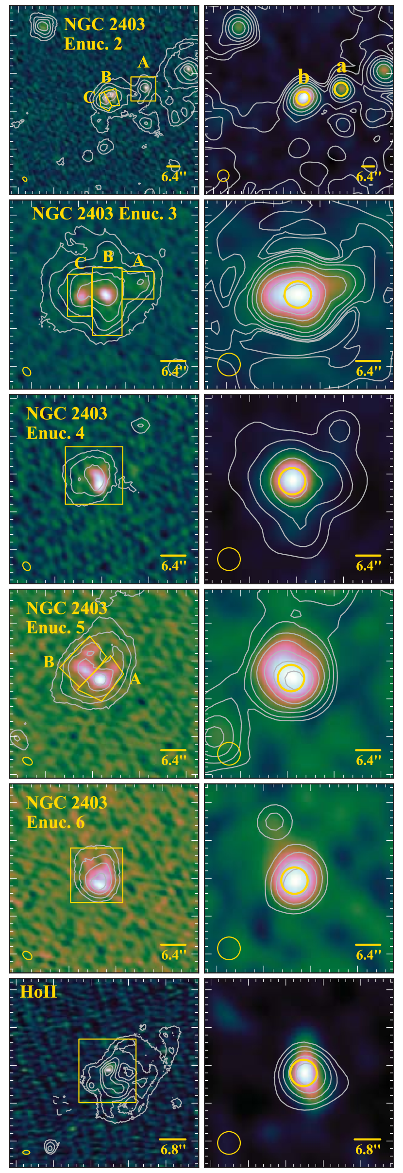
Figure 1.— Continued

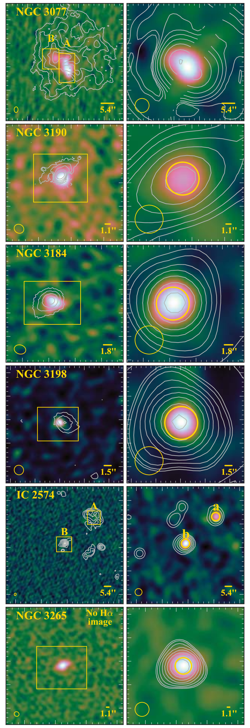
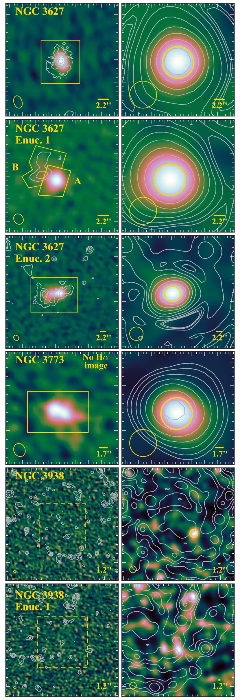
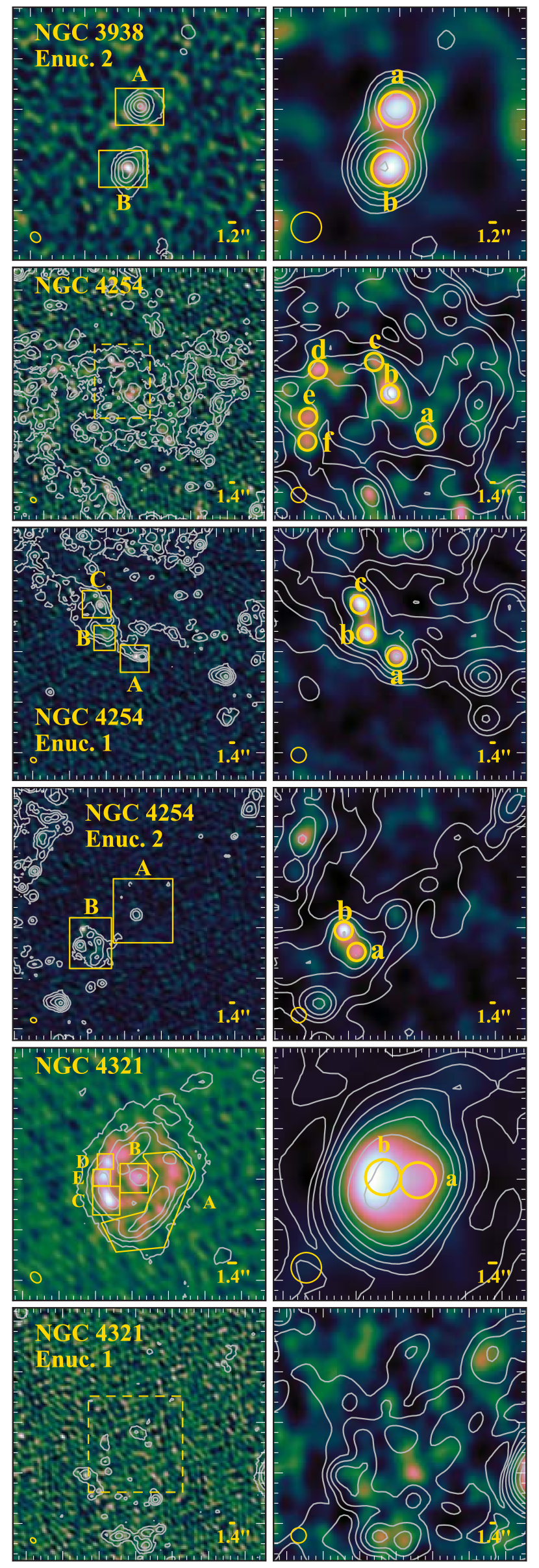
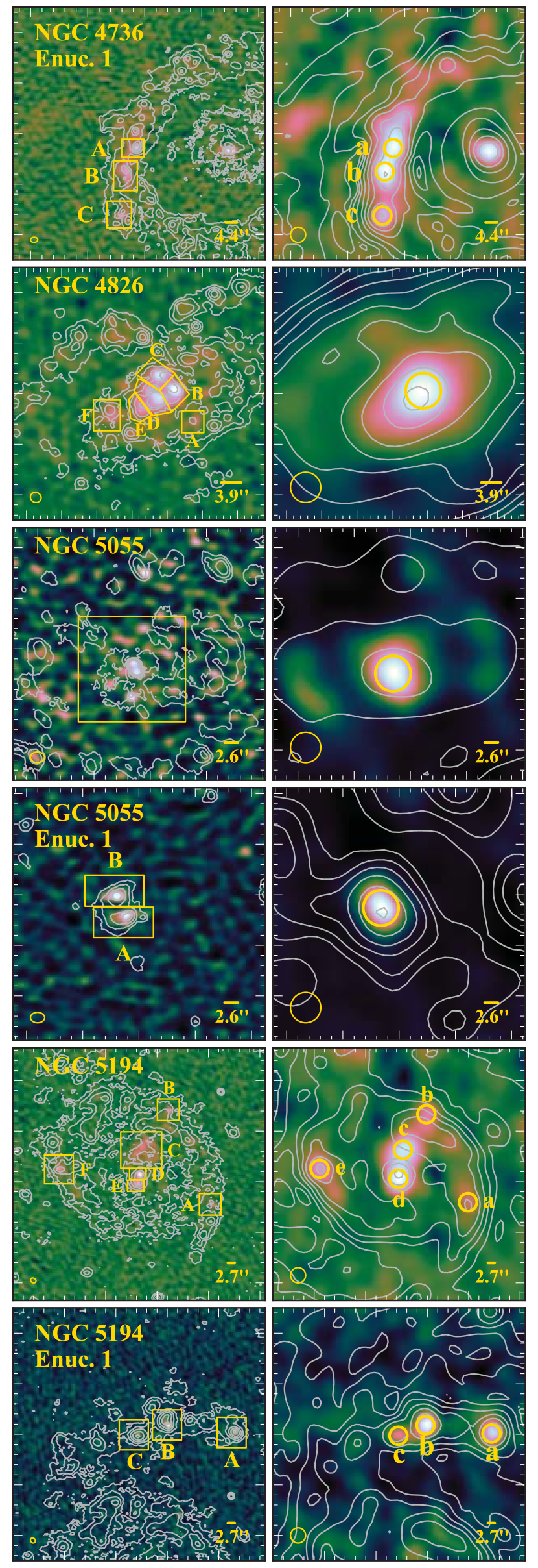
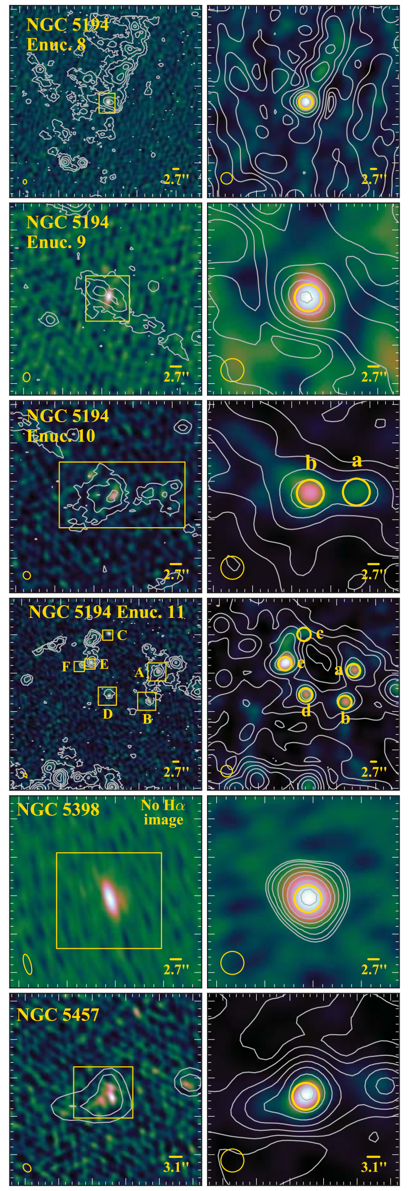
Figure 1.— Continued

Figure 1.— Continued

Figure 1.— Continued

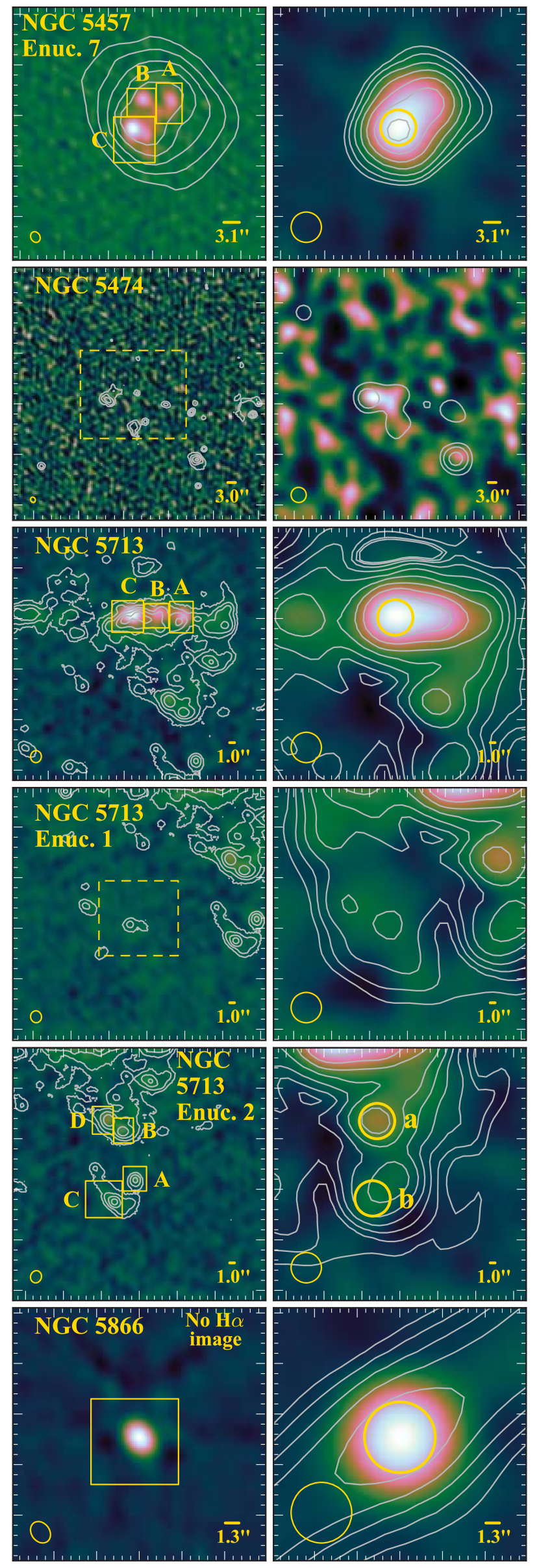
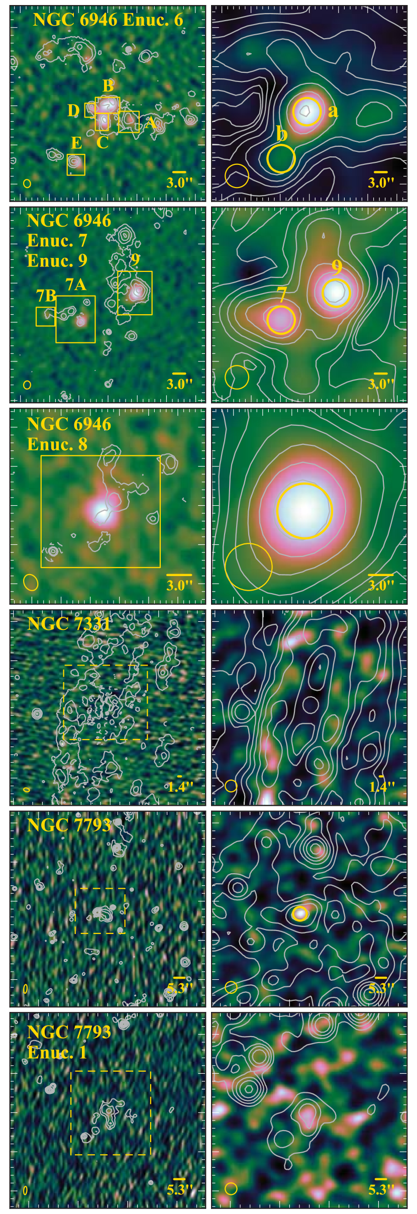
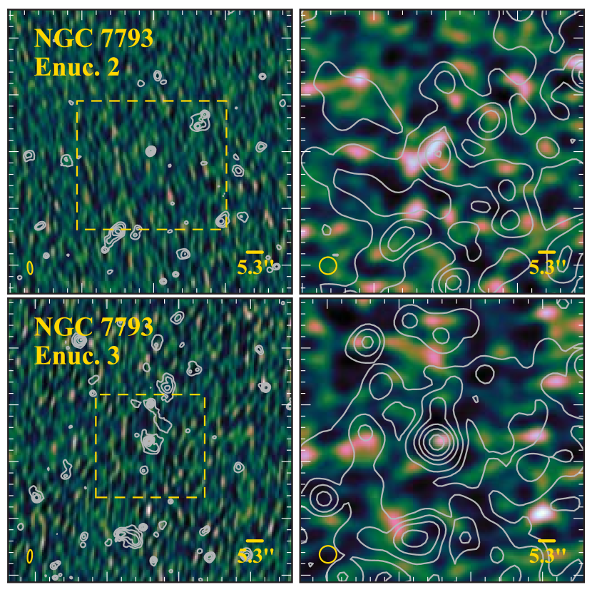
Figure 1.— Continued

Figure 1.— Continued

Figure 1.— Continued

Figure 1.— Continued

Figure 1.— Continued

Table 5Source Photometry

Source ID	R.A.	Decl.	$S_{\mathrm{33\,GHz}}$	$f_{\mathrm{H_{\alpha}}}/10^{-13}$	$r_{\mathrm{G}}$
	(J2000)	(J2000)	(mJy)	(erg s-1 cm-2)	(kpc)
NGC 0337 A	$00~{}59~{}50.00$	$-07~{}34~{}34.7$	$0.57\pm 0.02$	$3.40\pm 0.68$	0.823
NGC 0337 B	$00~{}59~{}50.74$	$-07~{}34~{}58.7$	$1.79\pm 0.06$	$6.18\pm 1.24$	2.100
NGC 0337 C	$00~{}59~{}51.77$	$-07~{}34~{}57.2$	$0.15\pm 0.01$	$1.29\pm 0.26$	2.946
NGC 0337 D	$00~{}59~{}51.87$	$-07~{}34~{}36.2$	$1.01\pm 0.03$	$5.12\pm 1.02$	3.699
NGC 0628 Enuc. 4	$01~{}36~{}35.71$	$+15~{}50~{}07.2$	$0.26\pm 0.01$	$1.15\pm 0.23$	7.611
NGC 0628 Enuc. 2	$01~{}36~{}37.65$	$+15~{}45~{}07.2$	$0.48\pm 0.02$	$1.04\pm 0.21$	4.468
NGC 0628 Enuc. 3	$01~{}36~{}38.92$	$+15~{}44~{}22.9$	$0.59\pm 0.03$	$2.14\pm 0.43$	5.715
NGC 0628	$01~{}36~{}43.26$	$+15~{}46~{}38.6$	$0.24\pm 0.02$	$3.26\pm 0.65$	1.210
NGC 0628 Enuc. 1	$01~{}36~{}45.24$	$+15~{}47~{}48.0$	$0.64\pm 0.03$	$1.74\pm 0.35$	2.463
NGC 0855	$02~{}14~{}03.55$	$+27~{}52~{}38.9$	$0.87\pm 0.03$	$\cdots$	0.036
NGC 0925	$02~{}27~{}17.67$	$+33~{}34~{}28.0$	$0.24\pm 0.01$	$8.59\pm 1.72$	1.314
NGC 1097 Enuc. 2	$02~{}46~{}14.28$	$-30~{}14~{}56.7$	$0.52\pm 0.02$	$\cdots$	7.990
NGC 1097 B	$02~{}46~{}18.31$	$-30~{}16~{}31.9$	$17.51\pm 0.53$	$\cdots$	0.885
NGC 1097 A	$02~{}46~{}18.98$	$-30~{}16~{}29.2$	$3.77\pm 0.12$	$\cdots$	0.030
NGC 1097 Enuc. 1	$02~{}46~{}21.19$	$-30~{}17~{}27.1$	$0.69\pm 0.02$	$\cdots$	4.883
NGC 1266	$03~{}16~{}00.76$	$-02~{}25~{}38.6$	$10.33\pm 0.31$	$\cdots$	0.168
NGC 1377	$03~{}36~{}39.11$	$-20~{}53~{}43.8$	$0.58\pm 0.03$	$\cdots$	5.952
IC 0342 A	$03~{}46~{}47.80$	$+68~{}05~{}46.0$	$18.05\pm 0.54$	$\cdots$	0.066
IC 0342 B	$03~{}46~{}48.61$	$+68~{}05~{}43.6$	$1.97\pm 0.07$	$\cdots$	0.039
IC 0342 C	$03~{}46~{}49.04$	$+68~{}05~{}46.0$	$3.87\pm 0.12$	$\cdots$	0.050
IC 0342 D	$03~{}46~{}49.20$	$+68~{}05~{}49.9$	$2.36\pm 0.08$	$\cdots$	0.093
NGC 1482	$03~{}54~{}39.07$	$-20~{}30~{}08.5$	$21.28\pm 0.64$	$\cdots$	0.272
NGC 2146 A	$06~{}18~{}33.93$	$+78~{}21~{}34.3$	$6.97\pm 0.21$	$\cdots$	2.122
NGC 2146 B	$06~{}18~{}35.22$	$+78~{}21~{}30.7$	$11.51\pm 0.35$	$\cdots$	1.348
NGC 2146 C	$06~{}18~{}36.61$	$+78~{}21~{}27.4$	$9.41\pm 0.28$	$\cdots$	0.581
NGC 2146 D	$06~{}18~{}37.50$	$+78~{}21~{}24.1$	$24.61\pm 0.74$	$\cdots$	0.105
NGC 2146 E	$06~{}18~{}38.79$	$+78~{}21~{}22.3$	$5.54\pm 0.17$	$\cdots$	0.615
NGC 2146 F	$06~{}18~{}38.99$	$+78~{}21~{}19.9$	$5.47\pm 0.17$	$\cdots$	0.955
NGC 2146 G	$06~{}18~{}39.38$	$+78~{}21~{}18.1$	$7.48\pm 0.23$	$\cdots$	1.278
NGC 2403 Enuc. 5 A	$07~{}36~{}19.69$	$+65~{}37~{}04.9$	$0.98\pm 0.03$	$4.39\pm 0.88$	3.484
NGC 2403 Enuc. 5 B	$07~{}36~{}20.32$	$+65~{}37~{}07.3$	$0.84\pm 0.03$	$3.67\pm 0.73$	3.396
NGC 2403 Enuc. 6	$07~{}36~{}28.69$	$+65~{}33~{}48.2$	$0.85\pm 0.03$	$3.84\pm 0.77$	5.406
NGC 2403 Enuc. 1 A	$07~{}36~{}42.01$	$+65~{}36~{}51.6$	$0.25\pm 0.02$	$0.54\pm 0.11$	1.085
NGC 2403 Enuc. 1 B	$07~{}36~{}45.60$	$+65~{}37~{}01.8$	$1.48\pm 0.05$	$8.48\pm 1.70$	1.214
NGC 2403	$07~{}36~{}46.95$	$+65~{}35~{}43.3$	$0.35\pm 0.01$	$9.31\pm 1.86$	0.802
NGC 2403 Enuc. 2 A	$07~{}36~{}49.16$	$+65~{}36~{}52.0$	$0.51\pm 0.02$	$2.30\pm 0.46$	1.123
NGC 2403 Enuc. 2 B	$07~{}36~{}52.12$	$+65~{}36~{}48.4$	$0.65\pm 0.02$	$2.91\pm 0.58$	1.263
NGC 2403 Enuc. 2 C	$07~{}36~{}52.65$	$+65~{}36~{}46.9$	$0.54\pm 0.02$	$2.56\pm 0.51$	1.276
NGC 2403 Enuc. 3 A	$07~{}37~{}05.21$	$+65~{}36~{}41.7$	$0.63\pm 0.03$	$2.16\pm 0.43$	2.637
NGC 2403 Enuc. 3 B	$07~{}37~{}06.85$	$+65~{}36~{}38.7$	$3.56\pm 0.11$	$12.79\pm 2.56$	2.793
NGC 2403 Enuc. 3 C	$07~{}37~{}07.92$	$+65~{}36~{}38.1$	$2.03\pm 0.06$	$5.34\pm 1.07$	2.920
NGC 2403 Enuc. 4	$07~{}37~{}18.14$	$+65~{}33~{}46.9$	$0.99\pm 0.03$	$3.26\pm 0.65$	3.463
Holmberg II	$08~{}19~{}13.12$	$+70~{}43~{}08.6$	$0.78\pm 0.03$	$5.44\pm 1.09$	0.742
NGC 2798	$09~{}17~{}22.83$	$+42~{}00~{}01.3$	$4.60\pm 0.14$	$10.83\pm 2.17$	0.221
NGC 2841	$09~{}22~{}02.67$	$+50~{}58~{}35.7$	$1.11\pm 0.03$	$0.51\pm 0.10$	0.155
NGC 2976 Enuc. 1 A	$09~{}47~{}05.14$	$+67~{}55~{}51.4$	$0.75\pm 0.03$	$1.08\pm 0.16$	1.425
NGC 2976 Enuc. 1 B	$09~{}47~{}07.53$	$+67~{}55~{}54.4$	$1.58\pm 0.05$	$5.40\pm 0.81$	1.205
NGC 2976 Enuc. 1 C	$09~{}47~{}07.85$	$+67~{}55~{}48.4$	$0.26\pm 0.02$	$0.86\pm 0.13$	1.114
NGC 2976 Enuc. 1 D	$09~{}47~{}08.28$	$+67~{}55~{}53.2$	$0.42\pm 0.02$	$2.54\pm 0.38$	1.141
NGC 2976	$09~{}47~{}13.54$	$+67~{}54~{}55.8$	$0.23\pm 0.02$	$5.07\pm 0.76$	0.412
NGC 2976 Enuc. 2 A	$09~{}47~{}23.04$	$+67~{}54~{}05.4$	$0.15\pm 0.02$	$0.93\pm 0.14$	1.205
NGC 2976 Enuc. 2 B	$09~{}47~{}23.52$	$+67~{}53~{}55.5$	$0.50\pm 0.03$	$1.59\pm 0.24$	1.368
NGC 2976 Enuc. 2 C	$09~{}47~{}23.89$	$+67~{}54~{}03.9$	$0.09\pm 0.02$	$0.24\pm 0.04$	1.287
NGC 2976 Enuc. 2 E	$09~{}47~{}24.37$	$+67~{}54~{}03.3$	$0.14\pm 0.02$	$0.57\pm 0.09$	1.335
NGC 2976 Enuc. 2 D	$09~{}47~{}24.37$	$+67~{}53~{}54.9$	$0.58\pm 0.03$	$2.92\pm 0.44$	1.426
NGC 3049	$09~{}54~{}49.56$	$+09~{}16~{}16.1$	$1.18\pm 0.04$	$3.44\pm 0.69$	0.103
NGC 3077 A	$10~{}03~{}18.82$	$+68~{}43~{}57.8$	$4.44\pm 0.14$	$7.85\pm 0.79$	0.086
NGC 3077 B	$10~{}03~{}19.82$	$+68~{}44~{}03.5$	$1.41\pm 0.05$	$5.96\pm 0.60$	0.080
NGC 3190	$10~{}18~{}05.64$	$+21~{}49~{}55.9$	$0.61\pm 0.02$	$0.38\pm 0.08$	0.098
NGC 3184	$10~{}18~{}16.89$	$+41~{}25~{}27.3$	$0.31\pm 0.02$	$0.60\pm 0.12$	0.043
NGC 3198	$10~{}19~{}55.01$	$+45~{}32~{}59.3$	$0.25\pm 0.02$	$0.25\pm 0.05$	0.161
IC 2574 A	$10~{}28~{}43.77$	$+68~{}28~{}27.8$	$0.67\pm 0.03$	$0.18\pm 0.04$	6.301
IC 2574 B	$10~{}28~{}48.40$	$+68~{}28~{}03.5$	$0.54\pm 0.02$	$4.23\pm 0.85$	5.254
NGC 3265	$10~{}31~{}06.77$	$+28~{}47~{}48.0$	$1.15\pm 0.04$	$\cdots$	0.087
NGC 3351 A	$10~{}43~{}57.64$	$+11~{}42~{}17.9$	$0.50\pm 0.02$	$2.26\pm 0.45$	0.247
NGC 3351 B	$10~{}43~{}57.66$	$+11~{}42~{}06.8$	$2.03\pm 0.06$	$6.20\pm 1.24$	0.285
NGC 3351 C	$10~{}43~{}57.76$	$+11~{}42~{}19.4$	$1.20\pm 0.04$	$2.13\pm 0.43$	0.294
NGC 3351 D	$10~{}43~{}58.05$	$+11~{}42~{}16.7$	$0.62\pm 0.03$	$1.99\pm 0.40$	0.351
NGC 3521 Enuc. 1	$11~{}05~{}46.86$	$-00~{}04~{}26.3$	$1.05\pm 0.05$	$1.50\pm 0.30$	10.282
NGC 3521 Enuc. 3	$11~{}05~{}48.60$	$+00~{}00~{}23.5$	$<$ 0.08	$1.35\pm 0.27$	9.547
NGC 3521 Enuc. 2	$11~{}05~{}49.38$	$-00~{}03~{}25.2$	$<$ 0.11	$4.17\pm 0.83$	4.350
NGC 3521	$11~{}05~{}49.76$	$-00~{}01~{}55.2$	$<$ 0.10	$9.48\pm 1.90$	2.512
NGC 3621	$11~{}18~{}16.88$	$-32~{}49~{}01.2$	$0.32\pm 0.03$	$\cdots$	0.671
NGC 3627	$11~{}20~{}15.02$	$+12~{}59~{}29.7$	$2.17\pm 0.07$	$2.03\pm 0.41$	0.032
NGC 3627 Enuc. 1 A	$11~{}20~{}16.28$	$+12~{}57~{}49.2$	$1.47\pm 0.05$	$0.30\pm 0.06$	4.699
NGC 3627 Enuc. 2	$11~{}20~{}16.38$	$+12~{}58~{}43.7$	$6.05\pm 0.18$	$5.64\pm 1.13$	2.661
NGC 3627 Enuc. 1 B	$11~{}20~{}16.47$	$+12~{}57~{}49.8$	$0.42\pm 0.02$	$0.84\pm 0.17$	4.736
NGC 3773	$11~{}38~{}13.10$	$+12~{}06~{}44.7$	$0.93\pm 0.03$	$\cdots$	0.118
NGC 3938 Enuc. 1	$11~{}52~{}44.51$	$+44~{}07~{}18.7$	$0.57\pm 0.03$	$2.77\pm 0.55$	4.978
NGC 3938	$11~{}52~{}48.83$	$+44~{}07~{}17.6$	$0.06\pm 0.02$	$2.47\pm 0.49$	0.637
NGC 3938 Enuc. 2 A	$11~{}52~{}59.94$	$+44~{}08~{}00.0$	$0.22\pm 0.02$	$0.63\pm 0.13$	11.053
NGC 3938 Enuc. 2 B	$11~{}53~{}00.22$	$+44~{}07~{}48.3$	$0.26\pm 0.02$	$0.73\pm 0.15$	11.077
NGC 4254 Enuc. 2 A	$12~{}18~{}45.22$	$+14~{}24~{}37.4$	$<$ 0.03	$0.89\pm 0.18$	5.111
NGC 4254 Enuc. 2 B	$12~{}18~{}46.15$	$+14~{}24~{}19.1$	$0.60\pm 0.02$	$1.98\pm 0.40$	4.667
NGC 4254 Enuc. 1 A	$12~{}18~{}49.20$	$+14~{}23~{}57.6$	$0.29\pm 0.02$	$0.70\pm 0.14$	4.449
NGC 4254 Enuc. 1 B	$12~{}18~{}50.07$	$+14~{}24~{}06.0$	$0.34\pm 0.02$	$1.11\pm 0.22$	3.966
NGC 4254	$12~{}18~{}50.16$	$+14~{}25~{}12.2$	$0.34\pm 0.02$	$6.05\pm 1.21$	1.031
NGC 4254 Enuc. 1 C	$12~{}18~{}50.19$	$+14~{}24~{}18.0$	$0.44\pm 0.02$	$1.44\pm 0.29$	3.158
NGC 4321 Enuc. 2	$12~{}22~{}49.92$	$+15~{}50~{}28.4$	$0.18\pm 0.01$	$1.16\pm 0.23$	7.991
NGC 4321 A	$12~{}22~{}54.63$	$+15~{}49~{}13.8$	$1.46\pm 0.05$	$2.75\pm 0.55$	0.568
NGC 4321 B	$12~{}22~{}54.94$	$+15~{}49~{}20.1$	$0.49\pm 0.02$	$0.82\pm 0.16$	0.086
NGC 4321 C	$12~{}22~{}55.32$	$+15~{}49~{}15.9$	$0.62\pm 0.03$	$0.75\pm 0.15$	0.641
NGC 4321 D	$12~{}22~{}55.34$	$+15~{}49~{}23.4$	$0.23\pm 0.02$	$0.11\pm 0.02$	0.503
NGC 4321 E	$12~{}22~{}55.38$	$+15~{}49~{}20.7$	$0.31\pm 0.02$	$0.28\pm 0.06$	0.547
NGC 4321 Enuc. 1	$12~{}22~{}58.53$	$+15~{}49~{}18.5$	$0.21\pm 0.01$	$1.96\pm 0.39$	4.155
NGC 4536 A	$12~{}34~{}26.92$	$+02~{}11~{}19.7$	$9.28\pm 0.28$	$4.41\pm 0.88$	0.273
NGC 4536 B	$12~{}34~{}27.30$	$+02~{}11~{}15.8$	$7.33\pm 0.22$	$2.38\pm 0.48$	0.277
NGC 4559 A	$12~{}35~{}56.18$	$+27~{}57~{}40.5$	$0.24\pm 0.01$	$3.22\pm 0.64$	1.395
NGC 4559 B	$12~{}35~{}56.39$	$+27~{}57~{}19.5$	$0.12\pm 0.01$	$2.99\pm 0.60$	2.028
NGC 4559 C	$12~{}35~{}58.45$	$+27~{}57~{}27.9$	$0.33\pm 0.01$	$3.60\pm 0.72$	0.563
NGC 4569	$12~{}36~{}49.80$	$+13~{}09~{}46.6$	$1.60\pm 0.05$	$9.57\pm 1.91$	0.037
NGC 4579	$12~{}37~{}43.52$	$+11~{}49~{}05.6$	$61.29\pm 1.84$	$4.56\pm 0.91$	0.105
NGC 4594	$12~{}39~{}59.42$	$-11~{}37~{}23.0$	$73.71\pm 2.21$	$1.85\pm 0.37$	0.052
NGC 4631 Enuc. 1	$12~{}41~{}40.73$	$+32~{}31~{}49.1$	$0.78\pm 0.03$	$6.78\pm 1.36$	13.672
NGC 4625	$12~{}41~{}50.72$	$+41~{}16~{}20.4$	$0.18\pm 0.01$	$3.32\pm 0.50$	1.078
NGC 4631 A	$12~{}42~{}03.34$	$+32~{}32~{}17.5$	$0.47\pm 0.02$	$0.17\pm 0.03$	3.135
NGC 4631 B	$12~{}42~{}03.58$	$+32~{}32~{}16.3$	$1.02\pm 0.03$	$0.29\pm 0.06$	3.384
NGC 4631 C	$12~{}42~{}04.14$	$+32~{}32~{}19.0$	$0.62\pm 0.02$	$0.49\pm 0.10$	2.701
NGC 4631 D	$12~{}42~{}04.19$	$+32~{}32~{}14.5$	$0.27\pm 0.02$	$0.26\pm 0.05$	3.823
NGC 4631 E	$12~{}42~{}04.26$	$+32~{}32~{}25.3$	$3.68\pm 0.11$	$1.06\pm 0.21$	1.755
NGC 4631 F	$12~{}42~{}05.05$	$+32~{}32~{}14.5$	$0.13\pm 0.02$	$0.09\pm 0.02$	3.863
NGC 4631 G	$12~{}42~{}05.07$	$+32~{}32~{}10.3$	$0.50\pm 0.02$	$0.81\pm 0.16$	5.072
NGC 4631 H	$12~{}42~{}05.59$	$+32~{}32~{}30.1$	$1.31\pm 0.04$	$1.16\pm 0.23$	1.485
NGC 4631 I	$12~{}42~{}06.23$	$+32~{}32~{}31.6$	$0.98\pm 0.03$	$0.65\pm 0.13$	1.501
NGC 4631 K	$12~{}42~{}07.18$	$+32~{}32~{}34.3$	$0.85\pm 0.03$	$0.43\pm 0.09$	1.858
NGC 4631 J	$12~{}42~{}07.25$	$+32~{}32~{}29.5$	$0.47\pm 0.02$	$0.18\pm 0.04$	0.494
NGC 4631 L	$12~{}42~{}07.68$	$+32~{}32~{}29.8$	$0.60\pm 0.02$	$0.26\pm 0.05$	0.359
NGC 4631 M	$12~{}42~{}07.84$	$+32~{}32~{}34.9$	$2.09\pm 0.06$	$0.45\pm 0.09$	1.826
NGC 4631 N	$12~{}42~{}08.18$	$+32~{}32~{}36.1$	$1.34\pm 0.04$	$0.30\pm 0.06$	2.102
NGC 4631 Enuc. 2 A	$12~{}42~{}21.44$	$+32~{}33~{}06.6$	$0.43\pm 0.02$	$1.80\pm 0.36$	10.046
NGC 4631 Enuc. 2 B	$12~{}42~{}21.92$	$+32~{}32~{}44.4$	$1.42\pm 0.04$	$6.93\pm 1.39$	6.592
NGC 4725 A	$12~{}50~{}26.56$	$+25~{}30~{}02.7$	$0.29\pm 0.01$	$<$ 0.02	0.043
NGC 4725 B	$12~{}50~{}28.48$	$+25~{}30~{}22.5$	$0.36\pm 0.02$	$0.04\pm 0.01$	1.935
NGC 4736	$12~{}50~{}53.03$	$+41~{}07~{}13.1$	$2.24\pm 0.07$	$2.72\pm 0.54$	0.019
NGC 4736 Enuc. 1 A	$12~{}50~{}56.33$	$+41~{}07~{}14.0$	$0.63\pm 0.03$	$1.61\pm 0.32$	0.842
NGC 4736 Enuc. 1 B	$12~{}50~{}56.65$	$+41~{}07~{}04.7$	$1.04\pm 0.04$	$2.12\pm 0.42$	0.926
NGC 4736 Enuc. 1 C	$12~{}50~{}56.86$	$+41~{}06~{}47.3$	$0.61\pm 0.03$	$1.51\pm 0.30$	1.144
NGC 4826 A	$12~{}56~{}43.10$	$+21~{}40~{}54.6$	$0.15\pm 0.01$	$0.57\pm 0.06$	0.438
NGC 4826 B	$12~{}56~{}43.41$	$+21~{}41~{}00.9$	$0.74\pm 0.03$	$2.10\pm 0.21$	0.114
NGC 4826 D	$12~{}56~{}43.62$	$+21~{}40~{}59.1$	$0.92\pm 0.03$	$4.96\pm 0.50$	0.066
NGC 4826 C	$12~{}56~{}43.64$	$+21~{}41~{}03.6$	$0.63\pm 0.02$	$1.03\pm 0.10$	0.156
NGC 4826 E	$12~{}56~{}43.86$	$+21~{}40~{}57.3$	$0.34\pm 0.02$	$1.08\pm 0.11$	0.110
NGC 4826 F	$12~{}56~{}44.29$	$+21~{}40~{}55.5$	$0.34\pm 0.02$	$0.69\pm 0.07$	0.240
NGC 5055	$13~{}15~{}49.36$	$+42~{}01~{}40.3$	$0.64\pm 0.03$	$4.90\pm 0.83$	0.309
NGC 5055 Enuc. 1 A	$13~{}15~{}58.24$	$+42~{}00~{}25.9$	$0.24\pm 0.02$	$1.05\pm 0.18$	5.686
NGC 5055 Enuc. 1 B	$13~{}15~{}58.40$	$+42~{}00~{}29.5$	$0.20\pm 0.02$	$0.88\pm 0.15$	5.549
NGC 5194 Enuc. 6 A	$13~{}29~{}39.35$	$+47~{}08~{}40.7$	$0.45\pm 0.02$	$1.06\pm 0.21$	12.306
NGC 5194 Enuc. 6 B	$13~{}29~{}39.35$	$+47~{}08~{}36.2$	$0.19\pm 0.01$	$0.40\pm 0.08$	12.445
NGC 5194 Enuc. 3 A	$13~{}29~{}43.69$	$+47~{}10~{}00.7$	$0.14\pm 0.01$	$0.41\pm 0.08$	7.689
NGC 5194 Enuc. 2 A	$13~{}29~{}44.07$	$+47~{}10~{}22.8$	$1.11\pm 0.04$	$5.10\pm 1.02$	6.866
NGC 5194 Enuc. 3 B	$13~{}29~{}44.54$	$+47~{}09~{}59.2$	$0.17\pm 0.01$	$1.10\pm 0.22$	7.291
NGC 5194 Enuc. 3 C	$13~{}29~{}45.16$	$+47~{}09~{}56.8$	$0.45\pm 0.02$	$0.95\pm 0.19$	7.052
NGC 5194 Enuc. 11 A	$13~{}29~{}47.05$	$+47~{}13~{}40.7$	$0.23\pm 0.01$	$1.12\pm 0.22$	4.946
NGC 5194 Enuc. 11 B	$13~{}29~{}47.55$	$+47~{}13~{}25.1$	$0.21\pm 0.01$	$0.36\pm 0.07$	4.357
NGC 5194 Enuc. 1 A	$13~{}29~{}49.42$	$+47~{}12~{}40.6$	$0.99\pm 0.03$	$1.53\pm 0.31$	2.570
NGC 5194 Enuc. 11 D	$13~{}29~{}49.55$	$+47~{}13~{}27.8$	$0.16\pm 0.01$	$0.28\pm 0.06$	4.049
NGC 5194 Enuc. 11 C	$13~{}29~{}49.55$	$+47~{}13~{}59.9$	$0.12\pm 0.01$	$0.03\pm 0.01$	5.215
NGC 5194 A	$13~{}29~{}49.93$	$+47~{}11~{}31.0$	$0.30\pm 0.02$	$0.54\pm 0.11$	1.875
NGC 5194 Enuc. 11 E	$13~{}29~{}50.47$	$+47~{}13~{}44.9$	$0.16\pm 0.01$	$0.39\pm 0.08$	4.631
NGC 5194 Enuc. 11 F	$13~{}29~{}50.94$	$+47~{}13~{}43.7$	$0.11\pm 0.01$	$0.10\pm 0.02$	4.595
NGC 5194 B	$13~{}29~{}51.55$	$+47~{}12~{}08.2$	$0.34\pm 0.02$	$0.98\pm 0.20$	1.043
NGC 5194 Enuc. 1 B	$13~{}29~{}52.04$	$+47~{}12~{}43.3$	$0.63\pm 0.02$	$2.83\pm 0.57$	2.308
NGC 5194 C	$13~{}29~{}52.58$	$+47~{}11~{}53.5$	$1.72\pm 0.05$	$3.97\pm 0.79$	0.402
NGC 5194 D	$13~{}29~{}52.70$	$+47~{}11~{}42.7$	$0.57\pm 0.02$	$1.66\pm 0.33$	0.012
NGC 5194 E	$13~{}29~{}52.76$	$+47~{}11~{}39.1$	$0.56\pm 0.02$	$1.31\pm 0.26$	0.148
NGC 5194 Enuc. 1 C	$13~{}29~{}53.19$	$+47~{}12~{}39.7$	$0.30\pm 0.02$	$1.73\pm 0.35$	2.348
NGC 5194 Enuc. 4	$13~{}29~{}55.49$	$+47~{}14~{}01.9$	$0.51\pm 0.02$	$0.13\pm 0.03$	6.205
NGC 5194 F	$13~{}29~{}55.82$	$+47~{}11~{}44.8$	$0.96\pm 0.03$	$1.95\pm 0.39$	1.920
NGC 5194 Enuc. 10	$13~{}29~{}56.52$	$+47~{}10~{}46.0$	$0.85\pm 0.03$	$2.65\pm 0.53$	2.743
NGC 5194 Enuc. 5	$13~{}29~{}59.63$	$+47~{}13~{}59.8$	$0.51\pm 0.02$	$0.10\pm 0.02$	7.755
NGC 5194 Enuc. 9	$13~{}29~{}59.84$	$+47~{}11~{}12.6$	$0.49\pm 0.02$	$1.22\pm 0.24$	4.166
NGC 5194 Enuc. 7 A	$13~{}30~{}00.91$	$+47~{}09~{}29.5$	$0.31\pm 0.02$	$1.03\pm 0.21$	6.159
NGC 5194 Enuc. 8	$13~{}30~{}01.51$	$+47~{}12~{}51.4$	$0.66\pm 0.03$	$1.45\pm 0.29$	6.659
NGC 5194 Enuc. 7 B	$13~{}30~{}02.38$	$+47~{}09~{}49.0$	$0.41\pm 0.02$	$2.39\pm 0.48$	6.323
NGC 5194 Enuc. 7 C	$13~{}30~{}02.77$	$+47~{}09~{}57.1$	$0.16\pm 0.02$	$1.16\pm 0.23$	6.364
NGC 5194 Enuc. 7 D	$13~{}30~{}03.47$	$+47~{}09~{}40.9$	$0.09\pm 0.02$	$0.78\pm 0.16$	6.952
NGC 5398	$14~{}01~{}20.13$	$-33~{}04~{}10.8$	$1.77\pm 0.06$	$\cdots$	1.406
NGC 5457 Enuc. 6 A	$14~{}02~{}28.24$	$+54~{}16~{}26.3$	$1.32\pm 0.04$	$7.80\pm 1.56$	15.713
NGC 5457 Enuc. 6 B	$14~{}02~{}29.64$	$+54~{}16~{}15.5$	$1.08\pm 0.04$	$3.33\pm 0.67$	15.547
NGC 5457 Enuc. 6 C	$14~{}02~{}30.60$	$+54~{}16~{}09.8$	$0.58\pm 0.02$	$2.80\pm 0.56$	15.414
NGC 5457 Enuc. 6 D	$14~{}02~{}30.63$	$+54~{}16~{}01.1$	$0.30\pm 0.02$	$1.16\pm 0.23$	15.567
NGC 5457 Enuc. 2	$14~{}02~{}55.10$	$+54~{}22~{}27.8$	$0.46\pm 0.02$	$2.61\pm 0.52$	6.428
NGC 5457 Enuc. 5	$14~{}03~{}01.17$	$+54~{}14~{}29.3$	$2.13\pm 0.07$	$10.36\pm 2.07$	13.102
NGC 5457 Enuc. 1 A	$14~{}03~{}11.16$	$+54~{}21~{}00.8$	$0.13\pm 0.01$	$0.77\pm 0.15$	0.473
NGC 5457	$14~{}03~{}12.43$	$+54~{}20~{}54.6$	$0.38\pm 0.02$	$1.62\pm 0.32$	0.092
NGC 5457 Enuc. 1 B	$14~{}03~{}12.53$	$+54~{}20~{}58.1$	$0.42\pm 0.02$	$1.69\pm 0.34$	0.044
NGC 5457 Enuc. 3 A	$14~{}03~{}38.32$	$+54~{}18~{}49.9$	$0.15\pm 0.02$	$1.04\pm 0.21$	9.334
NGC 5457 Enuc. 3 B	$14~{}03~{}39.86$	$+54~{}18~{}56.8$	$0.75\pm 0.03$	$2.67\pm 0.53$	9.645
NGC 5457 Enuc. 3 C	$14~{}03~{}41.40$	$+54~{}19~{}04.3$	$7.11\pm 0.21$	$17.84\pm 3.57$	9.964
NGC 5457 Enuc. 3 D	$14~{}03~{}42.98$	$+54~{}19~{}24.7$	$0.47\pm 0.03$	$0.54\pm 0.11$	10.133
NGC 5457 Enuc. 4 A	$14~{}03~{}51.90$	$+54~{}21~{}52.5$	$0.13\pm 0.01$	$0.75\pm 0.15$	12.107
NGC 5457 Enuc. 4 B	$14~{}03~{}53.07$	$+54~{}21~{}56.1$	$0.16\pm 0.01$	$0.60\pm 0.12$	12.471
NGC 5457 Enuc. 4 C	$14~{}03~{}53.13$	$+54~{}22~{}06.6$	$0.55\pm 0.02$	$2.40\pm 0.48$	12.520
NGC 5457 Enuc. 4 D	$14~{}03~{}53.99$	$+54~{}22~{}11.4$	$0.43\pm 0.02$	$1.83\pm 0.37$	12.797
NGC 5457 Enuc. 7 A	$14~{}04~{}28.61$	$+54~{}23~{}52.7$	$0.83\pm 0.03$	$4.66\pm 0.93$	23.671
NGC 5457 Enuc. 7 B	$14~{}04~{}29.23$	$+54~{}23~{}53.0$	$0.77\pm 0.03$	$4.10\pm 0.82$	23.857
NGC 5457 Enuc. 7 C	$14~{}04~{}29.47$	$+54~{}23~{}47.3$	$2.28\pm 0.07$	$4.87\pm 0.97$	23.901
NGC 5474	$14~{}05~{}00.29$	$+53~{}39~{}56.3$	$0.03\pm 0.01$	$2.73\pm 0.55$	0.540
NGC 5713 Enuc. 2 A	$14~{}40~{}10.56$	$-00~{}17~{}47.6$	$0.12\pm 0.01$	$0.13\pm 0.03$	3.251
NGC 5713 A	$14~{}40~{}10.74$	$-00~{}17~{}19.8$	$1.27\pm 0.04$	$0.49\pm 0.10$	1.324
NGC 5713 Enuc. 2 B	$14~{}40~{}10.74$	$-00~{}17~{}38.0$	$0.21\pm 0.02$	$0.43\pm 0.09$	2.252
NGC 5713 Enuc. 2 C	$14~{}40~{}10.88$	$-00~{}17~{}52.1$	$0.19\pm 0.02$	$0.36\pm 0.07$	3.473
NGC 5713 Enuc. 2 D	$14~{}40~{}10.94$	$-00~{}17~{}36.2$	$0.26\pm 0.02$	$0.43\pm 0.09$	1.915
NGC 5713 B	$14~{}40~{}11.06$	$-00~{}17~{}19.2$	$1.29\pm 0.04$	$0.93\pm 0.19$	0.774
NGC 5713 C	$14~{}40~{}11.40$	$-00~{}17~{}19.5$	$2.75\pm 0.08$	$1.53\pm 0.31$	0.184
NGC 5713 Enuc. 1	$14~{}40~{}12.08$	$-00~{}17~{}50.5$	$<$ 0.03	$0.43\pm 0.09$	3.371
NGC 5866	$15~{}06~{}29.50$	$+55~{}45~{}47.4$	$4.09\pm 0.12$	$\cdots$	0.102
NGC 6946 Enuc. 4 A	$20~{}34~{}19.16$	$+60~{}10~{}03.9$	$0.69\pm 0.02$	$\cdots$	9.184
NGC 6946 Enuc. 4 B	$20~{}34~{}19.88$	$+60~{}10~{}06.6$	$1.56\pm 0.05$	$\cdots$	9.033
NGC 6946 Enuc. 4 C	$20~{}34~{}21.41$	$+60~{}10~{}18.0$	$0.69\pm 0.02$	$\cdots$	8.806
NGC 6946 Enuc. 4 D	$20~{}34~{}22.70$	$+60~{}10~{}33.9$	$1.33\pm 0.04$	$\cdots$	8.743
NGC 6946 Enuc. 8	$20~{}34~{}32.28$	$+60~{}10~{}19.0$	$1.51\pm 0.05$	$5.98\pm 1.20$	6.116
NGC 6946 Enuc. 5	$20~{}34~{}39.36$	$+60~{}04~{}53.3$	$0.48\pm 0.02$	$7.01\pm 1.40$	9.673
NGC 6946 Enuc. 3 A	$20~{}34~{}49.83$	$+60~{}12~{}40.4$	$0.24\pm 0.01$	$2.45\pm 0.49$	7.734
NGC 6946 Enuc. 3 B	$20~{}34~{}51.19$	$+60~{}12~{}42.2$	$0.20\pm 0.01$	$2.31\pm 0.46$	7.722
NGC 6946 A	$20~{}34~{}51.30$	$+60~{}09~{}38.6$	$1.39\pm 0.05$	$4.20\pm 0.84$	0.983
NGC 6946 Enuc. 3 C	$20~{}34~{}52.20$	$+60~{}12~{}43.7$	$0.47\pm 0.02$	$7.15\pm 1.43$	7.730
NGC 6946 B	$20~{}34~{}52.26$	$+60~{}09~{}14.3$	$14.17\pm 0.43$	$15.37\pm 3.07$	0.016
NGC 6946 C	$20~{}34~{}52.82$	$+60~{}09~{}30.2$	$0.52\pm 0.03$	$1.60\pm 0.32$	0.591
NGC 6946 Enuc. 6 A	$20~{}35~{}05.24$	$+60~{}10~{}56.4$	$0.13\pm 0.02$	$2.22\pm 0.44$	4.666
NGC 6946 Enuc. 6 B	$20~{}35~{}06.04$	$+60~{}11~{}00.0$	$0.51\pm 0.02$	$2.45\pm 0.49$	4.886
NGC 6946 Enuc. 6 C	$20~{}35~{}06.20$	$+60~{}10~{}56.4$	$0.35\pm 0.02$	$1.66\pm 0.33$	4.823
NGC 6946 Enuc. 6 D	$20~{}35~{}06.56$	$+60~{}10~{}59.1$	$0.11\pm 0.02$	$0.91\pm 0.18$	4.949
NGC 6946 Enuc. 6 E	$20~{}35~{}07.05$	$+60~{}10~{}45.3$	$0.20\pm 0.02$	$1.21\pm 0.24$	4.717
NGC 6946 Enuc. 9	$20~{}35~{}11.09$	$+60~{}08~{}57.5$	$1.48\pm 0.05$	$8.40\pm 1.68$	5.071
NGC 6946 Enuc. 7 A	$20~{}35~{}12.93$	$+60~{}08~{}50.2$	$0.81\pm 0.03$	$3.27\pm 0.65$	5.630
NGC 6946 Enuc. 7 B	$20~{}35~{}14.10$	$+60~{}08~{}51.7$	$0.13\pm 0.02$	$0.74\pm 0.15$	5.916
NGC 6946 Enuc. 1	$20~{}35~{}16.76$	$+60~{}11~{}00.3$	$0.81\pm 0.03$	$7.72\pm 1.54$	6.985
NGC 6946 Enuc. 2 A	$20~{}35~{}23.61$	$+60~{}09~{}48.9$	$0.36\pm 0.02$	$5.20\pm 1.04$	8.131
NGC 6946 Enuc. 2 B	$20~{}35~{}25.50$	$+60~{}09~{}58.8$	$1.96\pm 0.06$	$25.89\pm 5.18$	8.626
NGC 7331	$22~{}37~{}02.96$	$+34~{}25~{}06.5$	$0.15\pm 0.04$	$6.15\pm 1.23$	2.930
NGC 7793 Enuc. 3	$23~{}57~{}48.87$	$-32~{}34~{}52.8$	$<$ 0.12	$5.65\pm 1.13$	0.992
NGC 7793 Enuc. 1	$23~{}57~{}49.44$	$-32~{}37~{}12.4$	$0.30\pm 0.03$	$7.08\pm 1.42$	2.953
NGC 7793	$23~{}57~{}49.56$	$-32~{}35~{}25.2$	$<$ 0.07	$3.63\pm 0.73$	0.093
NGC 7793 Enuc. 2	$23~{}57~{}55.74$	$-32~{}35~{}22.3$	$<$ 0.07	$5.67\pm 1.13$	1.468

Table 6Source Photometry at 7″ Resolution

Source ID	R.A.	Decl.	$S_{\mathrm{33\,GHz}}$	$f_{\mathrm{H_{\alpha}}}/10^{-13}$	$f_{\mathrm{24\,\micron}}$	$r_{\mathrm{G}}$
	(J2000)	(J2000)	(mJy)	(erg s-1 cm-2)	(mJy)	(kpc)
NGC 0337 a	$00~{}59~{}50.02$	$-07~{}34~{}33.9$	$0.23\pm 0.01$	$1.50\pm 0.30$	$48.04\pm 2.40$	0.945
NGC 0337 b	$00~{}59~{}50.68$	$-07~{}34~{}57.6$	$0.62\pm 0.02$	$1.72\pm 0.34$	$80.48\pm 4.02$	1.966
NGC 0337 c	$00~{}59~{}51.99$	$-07~{}34~{}54.9$	$0.10\pm 0.01$	$0.52\pm 0.10$	$8.54\pm 0.43$	3.227
NGC 0337 d	$00~{}59~{}52.16$	$-07~{}34~{}38.2$	$0.22\pm 0.01$	$1.32\pm 0.26$	$24.25\pm 1.21$	4.061
NGC 0628 Enuc. 4	$01~{}36~{}35.72$	$+15~{}50~{}07.2$	$0.12\pm 0.01$	$0.49\pm 0.10$	$10.30\pm 0.51$	7.608
NGC 0628 Enuc. 2	$01~{}36~{}37.65$	$+15~{}45~{}07.2$	$0.18\pm 0.02$	$0.43\pm 0.09$	$42.11\pm 2.11$	4.468
NGC 0628 Enuc. 3	$01~{}36~{}38.78$	$+15~{}44~{}23.2$	$0.19\pm 0.03$	$0.78\pm 0.16$	$31.08\pm 1.55$	5.720
NGC 0628	$01~{}36~{}41.70$	$+15~{}46~{}59.0$	$<$ 0.06	$0.06\pm 0.01$	$2.37\pm 0.12$	0.071
NGC 0628 Enuc. 1	$01~{}36~{}45.27$	$+15~{}47~{}48.3$	$0.29\pm 0.03$	$0.71\pm 0.14$	$78.59\pm 3.93$	2.478
NGC 0855	$02~{}14~{}03.68$	$+27~{}52~{}37.9$	$0.21\pm 0.01$	$\cdots$	$19.62\pm 0.98$	0.202
NGC 0925	$02~{}27~{}17.00$	$+33~{}34~{}43.0$	$<$ 0.04	$0.30\pm 0.06$	$3.40\pm 0.17$	0.183
NGC 1097 Enuc. 2	$02~{}46~{}14.40$	$-30~{}15~{}04.0$	$0.05\pm 0.01$	$\cdots$	$3.51\pm 0.18$	7.435
NGC 1097	$02~{}46~{}18.98$	$-30~{}16~{}28.8$	$2.30\pm 0.08$	$\cdots$	$158.45\pm 7.92$	0.020
NGC 1097 Enuc. 1 a	$02~{}46~{}22.56$	$-30~{}17~{}29.9$	$0.08\pm 0.01$	$\cdots$	$12.30\pm 0.62$	5.416
NGC 1097 Enuc. 1 b	$02~{}46~{}22.93$	$-30~{}17~{}48.1$	$0.12\pm 0.01$	$\cdots$	$11.02\pm 0.55$	6.817
NGC 1097 Enuc. 1 c	$02~{}46~{}24.06$	$-30~{}17~{}50.9$	$0.07\pm 0.01$	$\cdots$	$8.52\pm 0.43$	7.392
NGC 1266	$03~{}16~{}00.76$	$-02~{}25~{}37.1$	$4.58\pm 0.15$	$\cdots$	$458.85\pm 22.94$	0.270
NGC 1377	$03~{}36~{}38.90$	$-20~{}54~{}06.0$	$<$ 0.08	$\cdots$	$705.71\pm 35.29$	0.580
NGC 1482	$03~{}54~{}38.97$	$-20~{}30~{}07.8$	$6.71\pm 0.21$	$\cdots$	$1394.77\pm 69.74$	0.124
NGC 2403 Enuc. 5	$07~{}36~{}19.84$	$+65~{}37~{}05.5$	$0.56\pm 0.02$	$2.21\pm 0.44$	$54.79\pm 2.74$	3.464
NGC 2403 Enuc. 6	$07~{}36~{}28.69$	$+65~{}33~{}49.4$	$0.30\pm 0.01$	$1.14\pm 0.23$	$9.36\pm 0.47$	5.380
NGC 2403 Enuc. 1 a	$07~{}36~{}42.06$	$+65~{}36~{}51.9$	$0.13\pm 0.01$	$0.15\pm 0.03$	$3.73\pm 0.19$	1.087
NGC 2403 Enuc. 1 b	$07~{}36~{}45.50$	$+65~{}37~{}00.9$	$0.55\pm 0.02$	$2.80\pm 0.56$	$87.21\pm 4.36$	1.192
NGC 2403 Enuc. 2 a	$07~{}36~{}49.11$	$+65~{}36~{}51.7$	$0.25\pm 0.02$	$0.68\pm 0.14$	$36.22\pm 1.81$	1.113
NGC 2403	$07~{}36~{}50.00$	$+65~{}36~{}04.0$	$<$ 0.03	$0.16\pm 0.03$	$3.39\pm 0.17$	0.000
NGC 2403 Enuc. 2 b	$07~{}36~{}52.36$	$+65~{}36~{}46.9$	$0.49\pm 0.02$	$2.12\pm 0.42$	$61.17\pm 3.06$	1.249
NGC 2403 Enuc. 3	$07~{}37~{}06.95$	$+65~{}36~{}39.0$	$1.62\pm 0.05$	$4.92\pm 0.98$	$294.85\pm 14.74$	2.811
NGC 2403 Enuc. 4	$07~{}37~{}18.19$	$+65~{}33~{}48.1$	$0.33\pm 0.01$	$0.74\pm 0.15$	$17.82\pm 0.89$	3.455
Holmberg II	$08~{}19~{}13.06$	$+70~{}43~{}08.0$	$0.21\pm 0.02$	$1.49\pm 0.30$	$16.70\pm 0.83$	0.738
NGC 2798	$09~{}17~{}22.85$	$+42~{}00~{}00.4$	$2.06\pm 0.06$	$4.46\pm 0.89$	$1132.59\pm 56.63$	0.144
NGC 2841	$09~{}22~{}02.67$	$+50~{}58~{}35.7$	$0.56\pm 0.02$	$0.24\pm 0.05$	$13.12\pm 0.66$	0.155
NGC 2976 Enuc. 1 a	$09~{}47~{}05.19$	$+67~{}55~{}52.0$	$0.35\pm 0.02$	$0.58\pm 0.12$	$27.97\pm 1.40$	1.420
NGC 2976 Enuc. 1 b	$09~{}47~{}07.64$	$+67~{}55~{}54.7$	$0.86\pm 0.03$	$3.09\pm 0.62$	$133.92\pm 6.70$	1.201
NGC 2976	$09~{}47~{}13.49$	$+67~{}54~{}54.0$	$0.09\pm 0.02$	$0.50\pm 0.10$	$7.49\pm 0.37$	0.462
NGC 2976 Enuc. 2 a	$09~{}47~{}23.83$	$+67~{}53~{}54.9$	$0.45\pm 0.02$	$1.90\pm 0.38$	$55.16\pm 2.76$	1.394
NGC 2976 Enuc. 2 b	$09~{}47~{}23.94$	$+67~{}54~{}02.1$	$0.21\pm 0.02$	$1.09\pm 0.22$	$23.23\pm 1.16$	1.310
NGC 3049	$09~{}54~{}49.56$	$+09~{}16~{}16.1$	$0.54\pm 0.02$	$1.18\pm 0.24$	$191.34\pm 11.56$	0.103
NGC 3190	$10~{}18~{}05.64$	$+21~{}49~{}55.9$	$0.26\pm 0.02$	$0.15\pm 0.03$	$31.69\pm 1.58$	0.098
NGC 3184	$10~{}18~{}16.94$	$+41~{}25~{}27.0$	$0.14\pm 0.01$	$0.25\pm 0.05$	$57.85\pm 2.89$	0.063
NGC 3198	$10~{}19~{}54.99$	$+45~{}32~{}59.3$	$0.12\pm 0.02$	$0.12\pm 0.02$	$184.89\pm 9.24$	0.116
IC 2574 a	$10~{}28~{}43.71$	$+68~{}28~{}26.3$	$0.28\pm 0.02$	$0.06\pm 0.01$	$5.22\pm 0.26$	6.253
IC 2574 b	$10~{}28~{}48.40$	$+68~{}28~{}03.5$	$0.24\pm 0.02$	$1.74\pm 0.35$	$20.86\pm 1.04$	5.254
NGC 3265	$10~{}31~{}06.77$	$+28~{}47~{}48.0$	$0.43\pm 0.02$	$\cdots$	$147.65\pm 7.38$	0.087
NGC 3351 a	$10~{}43~{}57.68$	$+11~{}42~{}08.0$	$0.77\pm 0.03$	$2.42\pm 0.48$	$316.70\pm 15.83$	0.230
NGC 3351 b	$10~{}43~{}57.80$	$+11~{}42~{}18.5$	$0.89\pm 0.03$	$2.23\pm 0.45$	$403.05\pm 20.15$	0.258
NGC 3521 Enuc. 1	$11~{}05~{}46.30$	$-00~{}04~{}09.0$	$<$ 0.11	$0.12\pm 0.02$	$7.32\pm 0.37$	9.929
NGC 3521 Enuc. 3	$11~{}05~{}47.60$	$+00~{}00~{}33.0$	$<$ 0.07	$0.10\pm 0.02$	$7.48\pm 0.37$	9.509
NGC 3521	$11~{}05~{}48.90$	$-00~{}02~{}06.0$	$<$ 0.05	$0.59\pm 0.12$	$14.37\pm 0.72$	0.625
NGC 3521 Enuc. 2 a	$11~{}05~{}49.34$	$-00~{}03~{}24.2$	$0.15\pm 0.03$	$0.24\pm 0.05$	$22.25\pm 1.11$	4.302
NGC 3521 Enuc. 2 b	$11~{}05~{}49.94$	$-00~{}03~{}55.9$	$0.11\pm 0.03$	$0.05\pm 0.01$	$2.97\pm 0.15$	6.044
NGC 3621	$11~{}18~{}16.00$	$-32~{}48~{}42.0$	$<$ 0.09	$\cdots$	$7.86\pm 0.39$	0.348
NGC 3627	$11~{}20~{}15.00$	$+12~{}59~{}29.4$	$1.07\pm 0.04$	$0.88\pm 0.18$	$257.22\pm 12.86$	0.028
NGC 3627 Enuc. 1	$11~{}20~{}16.32$	$+12~{}57~{}49.2$	$0.85\pm 0.03$	$0.39\pm 0.08$	$177.00\pm 8.85$	4.712
NGC 3627 Enuc. 2	$11~{}20~{}16.46$	$+12~{}58~{}43.4$	$1.93\pm 0.06$	$0.92\pm 0.18$	$496.59\pm 24.83$	2.746
NGC 3773	$11~{}38~{}13.02$	$+12~{}06~{}43.8$	$0.38\pm 0.02$	$\cdots$	$60.04\pm 3.00$	0.023
NGC 3938	$11~{}52~{}48.19$	$+44~{}07~{}05.9$	$0.08\pm 0.01$	$0.07\pm 0.01$	$3.39\pm 0.17$	1.407
NGC 3938	$11~{}52~{}49.50$	$+44~{}07~{}14.0$	$<$ 0.04	$0.07\pm 0.01$	$5.68\pm 0.28$	0.140
NGC 3938 Enuc. 2 a	$11~{}53~{}00.06$	$+44~{}08~{}00.0$	$0.10\pm 0.02$	$0.29\pm 0.06$	$7.92\pm 0.40$	11.158
NGC 3938 Enuc. 2 b	$11~{}53~{}00.19$	$+44~{}07~{}48.3$	$0.11\pm 0.02$	$0.34\pm 0.07$	$22.10\pm 1.10$	11.049
NGC 4254 Enuc. 2 a	$12~{}18~{}45.78$	$+14~{}24~{}10.4$	$0.09\pm 0.01$	$0.36\pm 0.07$	$13.60\pm 0.68$	5.342
NGC 4254 Enuc. 2 b	$12~{}18~{}46.13$	$+14~{}24~{}18.8$	$0.12\pm 0.01$	$0.18\pm 0.04$	$11.38\pm 0.57$	4.698
NGC 4254 a	$12~{}18~{}48.68$	$+14~{}24~{}42.5$	$0.07\pm 0.02$	$0.45\pm 0.09$	$33.20\pm 1.66$	1.553
NGC 4254 Enuc. 1 a	$12~{}18~{}49.20$	$+14~{}23~{}57.9$	$0.12\pm 0.02$	$0.23\pm 0.05$	$22.90\pm 1.15$	4.428
NGC 4254 b	$12~{}18~{}49.67$	$+14~{}24~{}59.0$	$0.11\pm 0.02$	$0.60\pm 0.12$	$54.75\pm 2.74$	0.111
NGC 4254 Enuc. 1 b	$12~{}18~{}50.01$	$+14~{}24~{}06.9$	$0.15\pm 0.02$	$0.49\pm 0.10$	$18.52\pm 0.93$	3.886
NGC 4254 c	$12~{}18~{}50.10$	$+14~{}25~{}11.6$	$0.06\pm 0.02$	$0.37\pm 0.07$	$27.57\pm 1.38$	0.960
NGC 4254 Enuc. 1 c	$12~{}18~{}50.19$	$+14~{}24~{}18.6$	$0.18\pm 0.02$	$0.46\pm 0.09$	$34.51\pm 1.73$	3.116
NGC 4254 d	$12~{}18~{}51.63$	$+14~{}25~{}08.6$	$0.12\pm 0.02$	$0.23\pm 0.05$	$16.04\pm 0.80$	2.344
NGC 4254 e	$12~{}18~{}51.90$	$+14~{}24~{}49.7$	$0.13\pm 0.02$	$0.40\pm 0.08$	$25.51\pm 1.28$	2.813
NGC 4254 f	$12~{}18~{}51.92$	$+14~{}24~{}40.1$	$0.14\pm 0.02$	$0.23\pm 0.05$	$11.52\pm 0.58$	3.149
NGC 4321 Enuc. 2 a	$12~{}22~{}48.84$	$+15~{}50~{}12.8$	$0.05\pm 0.01$	$0.14\pm 0.03$	$8.59\pm 0.43$	8.305
NGC 4321 Enuc. 2 b	$12~{}22~{}49.90$	$+15~{}50~{}27.8$	$0.05\pm 0.01$	$0.15\pm 0.03$	$6.48\pm 0.32$	7.979
NGC 4321 Enuc. 2 c	$12~{}22~{}50.65$	$+15~{}50~{}27.2$	$0.04\pm 0.01$	$0.07\pm 0.01$	$4.81\pm 0.24$	7.285
NGC 4321 a	$12~{}22~{}54.65$	$+15~{}49~{}19.8$	$0.45\pm 0.02$	$0.80\pm 0.16$	$89.71\pm 4.49$	0.284
NGC 4321 b	$12~{}22~{}55.13$	$+15~{}49~{}20.4$	$0.63\pm 0.03$	$0.89\pm 0.18$	$124.94\pm 6.25$	0.270
NGC 4321 Enuc. 1	$12~{}22~{}58.90$	$+15~{}49~{}35.0$	$<$ 0.03	$0.10\pm 0.02$	$4.82\pm 0.24$	4.520
NGC 4536	$12~{}34~{}27.06$	$+02~{}11~{}18.2$	$4.90\pm 0.15$	$2.03\pm 0.41$	$1010.56\pm 50.53$	0.126
NGC 4559 a	$12~{}35~{}56.27$	$+27~{}57~{}40.5$	$0.08\pm 0.01$	$0.76\pm 0.15$	$10.30\pm 0.52$	1.304
NGC 4559 b	$12~{}35~{}56.46$	$+27~{}57~{}21.3$	$0.05\pm 0.01$	$0.57\pm 0.11$	$6.25\pm 0.31$	1.880
NGC 4559 c	$12~{}35~{}58.47$	$+27~{}57~{}29.7$	$0.11\pm 0.01$	$0.72\pm 0.14$	$18.98\pm 0.95$	0.608
NGC 4569	$12~{}36~{}49.80$	$+13~{}09~{}46.6$	$0.51\pm 0.03$	$2.96\pm 0.59$	$326.78\pm 16.34$	0.037
NGC 4579	$12~{}37~{}43.52$	$+11~{}49~{}05.6$	$30.13\pm 0.91$	$1.98\pm 0.40$	$101.01\pm 5.05$	0.105
NGC 4594	$12~{}39~{}59.42$	$-11~{}37~{}23.0$	$36.58\pm 1.10$	$0.77\pm 0.15$	$35.64\pm 1.78$	0.052
NGC 4631 Enuc. 1	$12~{}41~{}40.47$	$+32~{}31~{}49.1$	$0.14\pm 0.01$	$0.82\pm 0.16$	$7.67\pm 0.38$	13.762
NGC 4625	$12~{}41~{}52.40$	$+41~{}16~{}24.0$	$<$ 0.03	$0.15\pm 0.03$	$4.77\pm 0.24$	0.139
NGC 4631 a	$12~{}42~{}03.43$	$+32~{}32~{}17.2$	$0.72\pm 0.03$	$0.35\pm 0.07$	$40.98\pm 2.05$	3.189
NGC 4631 b	$12~{}42~{}03.98$	$+32~{}32~{}16.0$	$0.58\pm 0.02$	$0.48\pm 0.10$	$86.71\pm 4.34$	3.435
NGC 4631 c	$12~{}42~{}04.31$	$+32~{}32~{}25.3$	$1.29\pm 0.04$	$0.27\pm 0.05$	$171.90\pm 8.59$	1.734
NGC 4631 d	$12~{}42~{}05.09$	$+32~{}32~{}10.6$	$0.26\pm 0.02$	$0.38\pm 0.08$	$46.49\pm 2.32$	4.988
NGC 4631 e	$12~{}42~{}05.57$	$+32~{}32~{}29.5$	$0.61\pm 0.02$	$0.41\pm 0.08$	$95.52\pm 4.78$	1.387
NGC 4631 f	$12~{}42~{}06.26$	$+32~{}32~{}31.9$	$0.51\pm 0.02$	$0.35\pm 0.07$	$75.60\pm 3.78$	1.566
NGC 4631 g	$12~{}42~{}07.47$	$+32~{}32~{}31.6$	$0.97\pm 0.03$	$0.32\pm 0.06$	$145.27\pm 7.26$	0.960
NGC 4631 h	$12~{}42~{}08.06$	$+32~{}32~{}34.9$	$1.29\pm 0.04$	$0.30\pm 0.06$	$276.81\pm 13.84$	1.769
NGC 4631 Enuc. 2 a	$12~{}42~{}21.42$	$+32~{}33~{}06.3$	$0.18\pm 0.01$	$0.69\pm 0.14$	$19.61\pm 0.98$	9.974
NGC 4631 Enuc. 2 b	$12~{}42~{}21.99$	$+32~{}32~{}45.0$	$0.36\pm 0.02$	$1.93\pm 0.39$	$42.30\pm 2.11$	6.651
NGC 4725 a	$12~{}50~{}26.56$	$+25~{}30~{}03.0$	$0.16\pm 0.01$	$<$ 0.01	$22.16\pm 1.11$	0.044
NGC 4725 b	$12~{}50~{}28.48$	$+25~{}30~{}21.9$	$0.19\pm 0.01$	$0.01\pm 0.00$	$0.30\pm 0.02$	1.921
NGC 4736	$12~{}50~{}53.05$	$+41~{}07~{}12.8$	$1.02\pm 0.04$	$0.56\pm 0.11$	$313.33\pm 15.67$	0.014
NGC 4736 Enuc. 1 a	$12~{}50~{}56.41$	$+41~{}07~{}14.3$	$0.35\pm 0.02$	$0.89\pm 0.18$	$93.24\pm 4.66$	0.864
NGC 4736 Enuc. 1 b	$12~{}50~{}56.70$	$+41~{}07~{}05.0$	$0.39\pm 0.02$	$0.74\pm 0.15$	$91.02\pm 4.55$	0.939
NGC 4736 Enuc. 1 c	$12~{}50~{}56.78$	$+41~{}06~{}47.6$	$0.26\pm 0.02$	$0.54\pm 0.11$	$93.76\pm 4.69$	1.123
NGC 4826	$12~{}56~{}43.56$	$+21~{}41~{}00.6$	$1.00\pm 0.03$	$3.44\pm 0.69$	$203.63\pm 10.18$	0.055
NGC 5055	$13~{}15~{}49.31$	$+42~{}01~{}45.1$	$0.12\pm 0.02$	$1.26\pm 0.25$	$41.37\pm 2.07$	0.009
NGC 5055 Enuc. 1	$13~{}15~{}58.32$	$+42~{}00~{}27.4$	$0.15\pm 0.02$	$0.64\pm 0.13$	$23.38\pm 1.17$	5.630
NGC 5194 Enuc. 6	$13~{}29~{}39.32$	$+47~{}08~{}40.7$	$0.21\pm 0.01$	$0.50\pm 0.10$	$26.64\pm 1.33$	12.321
NGC 5194 Enuc. 2	$13~{}29~{}44.10$	$+47~{}10~{}23.4$	$0.39\pm 0.02$	$1.40\pm 0.28$	$102.84\pm 5.14$	6.834
NGC 5194 Enuc. 3	$13~{}29~{}45.13$	$+47~{}09~{}57.4$	$0.25\pm 0.01$	$0.67\pm 0.13$	$65.69\pm 3.28$	7.048
NGC 5194 Enuc. 11 a	$13~{}29~{}47.14$	$+47~{}13~{}41.3$	$0.10\pm 0.01$	$0.43\pm 0.09$	$14.18\pm 0.71$	4.941
NGC 5194 Enuc. 11 b	$13~{}29~{}47.58$	$+47~{}13~{}24.8$	$0.09\pm 0.01$	$0.13\pm 0.03$	$10.22\pm 0.51$	4.340
NGC 5194 Enuc. 1 a	$13~{}29~{}49.51$	$+47~{}12~{}40.3$	$0.38\pm 0.02$	$0.58\pm 0.12$	$84.19\pm 4.21$	2.534
NGC 5194 Enuc. 11 d	$13~{}29~{}49.58$	$+47~{}13~{}28.7$	$0.07\pm 0.01$	$0.12\pm 0.02$	$15.18\pm 0.76$	4.078
NGC 5194 Enuc. 11 c	$13~{}29~{}49.67$	$+47~{}14~{}00.2$	$0.06\pm 0.01$	$0.10\pm 0.02$	$2.83\pm 0.14$	5.221
NGC 5194 c	$13~{}29~{}50.02$	$+47~{}11~{}31.9$	$0.16\pm 0.01$	$0.32\pm 0.06$	$51.41\pm 2.57$	1.804
NGC 5194 Enuc. 11 e	$13~{}29~{}50.64$	$+47~{}13~{}44.9$	$0.13\pm 0.01$	$0.26\pm 0.05$	$23.92\pm 1.20$	4.633
NGC 5194 b	$13~{}29~{}51.64$	$+47~{}12~{}06.7$	$0.22\pm 0.01$	$0.60\pm 0.12$	$36.69\pm 1.83$	0.977
NGC 5194 Enuc. 1 b	$13~{}29~{}52.07$	$+47~{}12~{}43.6$	$0.27\pm 0.02$	$0.94\pm 0.19$	$76.18\pm 3.81$	2.322
NGC 5194 e	$13~{}29~{}52.55$	$+47~{}11~{}52.6$	$0.45\pm 0.02$	$0.76\pm 0.15$	$30.02\pm 1.50$	0.365
NGC 5194 d	$13~{}29~{}52.73$	$+47~{}11~{}40.6$	$0.52\pm 0.02$	$1.86\pm 0.37$	$98.02\pm 4.90$	0.092
NGC 5194 Enuc. 1 c	$13~{}29~{}53.13$	$+47~{}12~{}39.4$	$0.14\pm 0.01$	$0.67\pm 0.13$	$33.13\pm 1.66$	2.323
NGC 5194 Enuc. 4 a	$13~{}29~{}53.93$	$+47~{}14~{}04.9$	$0.08\pm 0.01$	$0.02\pm 0.00$	$10.79\pm 0.54$	5.880
NGC 5194 Enuc. 10 a	$13~{}29~{}55.35$	$+47~{}10~{}47.2$	$0.09\pm 0.02$	$0.18\pm 0.04$	$20.28\pm 1.01$	2.336
NGC 5194 Enuc. 4 b	$13~{}29~{}55.49$	$+47~{}14~{}01.6$	$0.19\pm 0.01$	$0.02\pm 0.00$	$34.81\pm 1.74$	6.193
NGC 5194 Enuc. 4 c	$13~{}29~{}55.61$	$+47~{}13~{}50.2$	$0.08\pm 0.01$	$0.02\pm 0.00$	$13.88\pm 0.69$	5.798
NGC 5194 a	$13~{}29~{}55.79$	$+47~{}11~{}45.1$	$0.34\pm 0.02$	$0.68\pm 0.14$	$108.62\pm 5.43$	1.906
NGC 5194 Enuc. 10 b	$13~{}29~{}56.52$	$+47~{}10~{}46.9$	$0.14\pm 0.02$	$0.39\pm 0.08$	$39.62\pm 1.98$	2.723
NGC 5194 Enuc. 4 d	$13~{}29~{}58.73$	$+47~{}14~{}09.4$	$0.07\pm 0.01$	$0.02\pm 0.00$	$23.43\pm 1.17$	7.696
NGC 5194 Enuc. 5	$13~{}29~{}59.60$	$+47~{}13~{}59.8$	$0.17\pm 0.02$	$0.02\pm 0.00$	$33.37\pm 1.67$	7.742
NGC 5194 Enuc. 9	$13~{}29~{}59.78$	$+47~{}11~{}12.3$	$0.20\pm 0.02$	$0.39\pm 0.08$	$53.25\pm 2.66$	4.131
NGC 5194 Enuc. 7 a	$13~{}30~{}01.03$	$+47~{}09~{}28.6$	$0.12\pm 0.02$	$0.39\pm 0.08$	$9.40\pm 0.47$	6.221
NGC 5194 Enuc. 8	$13~{}30~{}01.48$	$+47~{}12~{}51.7$	$0.29\pm 0.02$	$0.62\pm 0.12$	$114.17\pm 5.71$	6.650
NGC 5194 Enuc. 7 b	$13~{}30~{}02.38$	$+47~{}09~{}48.7$	$0.20\pm 0.02$	$1.04\pm 0.21$	$52.45\pm 2.62$	6.329
NGC 5194 Enuc. 7 c	$13~{}30~{}03.47$	$+47~{}09~{}40.3$	$<$ 0.06	$0.41\pm 0.08$	$14.98\pm 0.75$	6.962
NGC 5398	$14~{}01~{}20.10$	$-33~{}04~{}09.2$	$0.69\pm 0.03$	$\cdots$	$104.29\pm 5.21$	1.381
NGC 5457 Enuc. 6 a	$14~{}02~{}28.20$	$+54~{}16~{}27.2$	$0.39\pm 0.02$	$1.80\pm 0.36$	$64.28\pm 3.21$	15.707
NGC 5457 Enuc. 6 b	$14~{}02~{}29.61$	$+54~{}16~{}15.8$	$0.44\pm 0.02$	$1.19\pm 0.24$	$60.68\pm 3.03$	15.550
NGC 5457 Enuc. 6 c	$14~{}02~{}30.57$	$+54~{}16~{}09.8$	$0.30\pm 0.02$	$1.15\pm 0.23$	$65.81\pm 3.29$	15.422
NGC 5457 Enuc. 2	$14~{}02~{}55.00$	$+54~{}22~{}27.5$	$0.16\pm 0.02$	$0.70\pm 0.14$	$25.18\pm 1.26$	6.451
NGC 5457 Enuc. 5	$14~{}03~{}01.20$	$+54~{}14~{}28.4$	$0.70\pm 0.03$	$2.39\pm 0.48$	$77.89\pm 3.89$	13.129
NGC 5457 Enuc. 1	$14~{}03~{}10.20$	$+54~{}20~{}57.8$	$0.05\pm 0.01$	$0.20\pm 0.04$	$13.50\pm 0.68$	0.744
NGC 5457	$14~{}03~{}12.53$	$+54~{}20~{}55.2$	$0.15\pm 0.01$	$0.41\pm 0.08$	$54.79\pm 2.74$	0.062
NGC 5457 Enuc. 3 a	$14~{}03~{}38.32$	$+54~{}18~{}51.4$	$0.07\pm 0.02$	$0.46\pm 0.09$	$15.42\pm 0.77$	9.307
NGC 5457 Enuc. 3 b	$14~{}03~{}39.89$	$+54~{}18~{}56.8$	$0.34\pm 0.02$	$0.97\pm 0.19$	$55.58\pm 2.78$	9.655
NGC 5457 Enuc. 3 c	$14~{}03~{}41.44$	$+54~{}19~{}04.9$	$2.85\pm 0.09$	$5.37\pm 1.07$	$621.47\pm 31.07$	9.964
NGC 5457 Enuc. 3 d	$14~{}03~{}42.91$	$+54~{}19~{}24.7$	$0.21\pm 0.02$	$0.27\pm 0.05$	$40.62\pm 2.03$	10.113
NGC 5457 Enuc. 4 a	$14~{}03~{}52.04$	$+54~{}21~{}52.5$	$0.10\pm 0.01$	$0.57\pm 0.11$	$7.21\pm 0.36$	12.149
NGC 5457 Enuc. 4 b	$14~{}03~{}53.00$	$+54~{}21~{}57.3$	$0.13\pm 0.01$	$0.65\pm 0.13$	$11.41\pm 0.57$	12.453
NGC 5457 Enuc. 4 c	$14~{}03~{}53.20$	$+54~{}22~{}06.3$	$0.28\pm 0.02$	$1.44\pm 0.29$	$40.88\pm 2.04$	12.540
NGC 5457 Enuc. 4 d	$14~{}03~{}53.99$	$+54~{}22~{}10.8$	$0.24\pm 0.02$	$1.02\pm 0.20$	$27.76\pm 1.39$	12.795
NGC 5457 Enuc. 7	$14~{}04~{}29.33$	$+54~{}23~{}47.6$	$1.12\pm 0.04$	$3.40\pm 0.68$	$55.41\pm 2.77$	23.861
NGC 5474	$14~{}05~{}01.30$	$+53~{}39~{}44.0$	$<$ 0.03	$0.09\pm 0.02$	$1.19\pm 0.06$	0.070
NGC 5713 Enuc. 2 a	$14~{}40~{}10.80$	$-00~{}17~{}35.5$	$0.27\pm 0.02$	$0.55\pm 0.11$	$60.40\pm 3.02$	1.984
NGC 5713 Enuc. 2 b	$14~{}40~{}10.86$	$-00~{}17~{}50.2$	$0.09\pm 0.01$	$0.26\pm 0.05$	$29.42\pm 1.47$	3.295
NGC 5713	$14~{}40~{}11.30$	$-00~{}17~{}27.0$	$0.35\pm 0.02$	$0.38\pm 0.08$	$51.77\pm 2.59$	0.795
NGC 5713	$14~{}40~{}11.36$	$-00~{}17~{}18.2$	$1.76\pm 0.06$	$0.99\pm 0.20$	$404.14\pm 20.21$	0.313
NGC 5866	$15~{}06~{}29.50$	$+55~{}45~{}47.7$	$2.01\pm 0.06$	$\cdots$	$21.43\pm 1.07$	0.051
NGC 6946 Enuc. 4 a	$20~{}34~{}19.84$	$+60~{}10~{}06.6$	$0.82\pm 0.03$	$\cdots$	$17.29\pm 0.86$	9.044
NGC 6946 Enuc. 4 b	$20~{}34~{}21.41$	$+60~{}10~{}17.7$	$0.34\pm 0.01$	$\cdots$	$1.05\pm 0.05$	8.801
NGC 6946 Enuc. 4 c	$20~{}34~{}22.74$	$+60~{}10~{}34.2$	$0.61\pm 0.02$	$\cdots$	$126.59\pm 6.33$	8.739
NGC 6946 Enuc. 8	$20~{}34~{}32.28$	$+60~{}10~{}19.3$	$0.56\pm 0.02$	$1.37\pm 0.27$	$81.70\pm 4.08$	6.122
NGC 6946 Enuc. 5 a	$20~{}34~{}37.15$	$+60~{}05~{}10.1$	$0.07\pm 0.01$	$0.64\pm 0.13$	$4.36\pm 0.22$	9.239
NGC 6946 Enuc. 5 b	$20~{}34~{}39.36$	$+60~{}04~{}52.4$	$0.16\pm 0.01$	$1.30\pm 0.26$	$10.92\pm 0.55$	9.704
NGC 6946 Enuc. 3 a	$20~{}34~{}49.86$	$+60~{}12~{}40.7$	$0.10\pm 0.01$	$1.16\pm 0.23$	$5.35\pm 0.27$	7.742
NGC 6946 a	$20~{}34~{}51.30$	$+60~{}09~{}39.2$	$0.49\pm 0.04$	$1.45\pm 0.29$	$75.91\pm 3.80$	1.005
NGC 6946 Enuc. 3 b	$20~{}34~{}52.24$	$+60~{}12~{}43.7$	$0.17\pm 0.01$	$2.38\pm 0.48$	$22.47\pm 1.12$	7.729
NGC 6946 b	$20~{}34~{}52.26$	$+60~{}09~{}14.3$	$5.36\pm 0.16$	$4.82\pm 0.96$	$2160.35\pm 108.02$	0.016
NGC 6946 c	$20~{}34~{}52.74$	$+60~{}09~{}30.5$	$0.24\pm 0.04$	$0.91\pm 0.18$	$45.06\pm 2.25$	0.601
NGC 6946 Enuc. 6 a	$20~{}35~{}06.08$	$+60~{}10~{}58.5$	$0.46\pm 0.02$	$2.94\pm 0.59$	$106.62\pm 5.33$	4.855
NGC 6946 Enuc. 6 b	$20~{}35~{}06.96$	$+60~{}10~{}46.5$	$0.12\pm 0.02$	$1.08\pm 0.22$	$43.73\pm 2.19$	4.728
NGC 6946 Enuc. 9	$20~{}35~{}11.09$	$+60~{}08~{}57.5$	$0.68\pm 0.03$	$3.29\pm 0.66$	$119.69\pm 5.98$	5.071
NGC 6946 Enuc. 7	$20~{}35~{}12.97$	$+60~{}08~{}50.5$	$0.33\pm 0.02$	$1.19\pm 0.24$	$73.65\pm 3.68$	5.637
NGC 6946 Enuc. 1	$20~{}35~{}16.80$	$+60~{}11~{}00.0$	$0.32\pm 0.02$	$2.73\pm 0.55$	$48.45\pm 2.42$	6.989
NGC 6946 Enuc. 2 a	$20~{}35~{}23.57$	$+60~{}09~{}48.9$	$0.15\pm 0.02$	$2.66\pm 0.53$	$17.88\pm 0.89$	8.120
NGC 6946 Enuc. 2 b	$20~{}35~{}25.38$	$+60~{}09~{}58.8$	$0.67\pm 0.03$	$7.44\pm 1.49$	$70.65\pm 3.53$	8.595
NGC 7331	$22~{}37~{}04.10$	$+34~{}24~{}56.0$	$<$ 0.10	$<$ 0.18	$17.10\pm 0.85$	0.000
NGC 7793 Enuc. 1	$23~{}57~{}48.80$	$-32~{}36~{}58.0$	$<$ 0.09	$0.62\pm 0.12$	$5.11\pm 0.26$	2.574
NGC 7793 Enuc. 3	$23~{}57~{}48.80$	$-32~{}34~{}52.0$	$<$ 0.11	$0.78\pm 0.16$	$29.99\pm 1.50$	1.016
NGC 7793	$23~{}57~{}49.20$	$-32~{}35~{}24.0$	$<$ 0.07	$0.55\pm 0.11$	$10.81\pm 0.54$	0.174
NGC 7793	$23~{}57~{}49.58$	$-32~{}35~{}25.6$	$<$ 0.07	$0.62\pm 0.12$	$15.14\pm 0.76$	0.081
NGC 7793 Enuc. 2	$23~{}57~{}56.10$	$-32~{}35~{}40.0$	$<$ 0.07	$0.22\pm 0.04$	$5.76\pm 0.29$	1.526

References

- Aniano et al. (2011) Aniano, G., Draine, B. T., Gordon, K. D., & Sandstrom, K. 2011, PASP, 123, 1218
- Bendo et al. (2015) Bendo, G. J., Baes, M., Bianchi, S., et al. 2015, MNRAS, 448, 135
- Ciardullo et al. (2002) Ciardullo, R., Feldmeier, J. J., Jacoby, G. H., et al. 2002, ApJ, 577, 31
- Condon (1992) Condon, J. J. 1992, ARA&A, 30, 575
- Condon & Yin (1990) Condon, J. J., & Yin, Q. F. 1990, ApJ, 357, 97
- Conway et al. (1990) Conway, J. E., Cornwell, T. J., & Wilkinson, P. N. 1990, MNRAS, 246, 490
- Cornwell (2008) Cornwell, T. J. 2008, IEEE Journal of Selected Topics in Signal Processing, 2, 793
- Dale et al. (1997) Dale, D. A., Giovanelli, R., Haynes, M. P., et al. 1997, AJ, 114, 455
- Dale et al. (2007) Dale, D. A., Gil de Paz, A., Gordon, K. D., et al. 2007, ApJ, 655, 863
- Dale et al. (2009) Dale, D. A., Cohen, S. A., Johnson, L. C., et al. 2009, ApJ, 703, 517
- de Jong et al. (1985) de Jong, T., Klein, U., Wielebinski, R., & Wunderlich, E. 1985, A&A, 147, L6
- de Vaucouleurs et al. (1991) de Vaucouleurs, G., de Vaucouleurs, A., Corwin, Jr., H. G., et al. 1991, Third Reference Catalogue of Bright Galaxies. Volume I: Explanations and references. Volume II: Data for galaxies between 0h and 12h. Volume III: Data for galaxies between 12h and 24h.
- Draine & Lazarian (1998a) Draine, B. T., & Lazarian, A. 1998a, ApJ, 494, L19+
- Draine & Lazarian (1998b) —. 1998b, ApJ, 508, 157
- Draine & Lazarian (1999) —. 1999, ApJ, 512, 740
- Engelbracht et al. (2008) Engelbracht, C. W., Rieke, G. H., Gordon, K. D., et al. 2008, ApJ, 678, 804
- Erickson (1957) Erickson, W. C. 1957, ApJ, 126, 480
- Freedman et al. (2001) Freedman, W. L., Madore, B. F., Gibson, B. K., et al. 2001, ApJ, 553, 47
- Green (2011) Green, D. A. 2011, Bulletin of the Astronomical Society of India, 39, 289
- Groves et al. (2012) Groves, B., Krause, O., Sandstrom, K., et al. 2012, MNRAS, 426, 892
- Helou et al. (1985) Helou, G., Soifer, B. T., & Rowan-Robinson, M. 1985, ApJ, 298, L7
- Hensley et al. (2015) Hensley, B., Murphy, E., & Staguhn, J. 2015, MNRAS, 449, 809
- Hensley et al. (2016) Hensley, B. S., Draine, B. T., & Meisner, A. M. 2016, ApJ, 827, 45
- Ho et al. (1997) Ho, L. C., Filippenko, A. V., & Sargent, W. L. W. 1997, ApJS, 112, 315
- Hughes et al. (2006) Hughes, A., Wong, T., Ekers, R., et al. 2006, MNRAS, 370, 363
- Jarrett et al. (2003) Jarrett, T. H., Chester, T., Cutri, R., Schneider, S. E., & Huchra, J. P. 2003, AJ, 125, 525
- Johnson et al. (2001) Johnson, K. E., Kobulnicky, H. A., Massey, P., & Conti, P. S. 2001, ApJ, 559, 864
- Kennicutt et al. (2011) Kennicutt, R. C., Calzetti, D., Aniano, G., et al. 2011, PASP, 123, 1347
- Kennicutt et al. (1989) Kennicutt, Jr., R. C., Keel, W. C., & Blaha, C. A. 1989, AJ, 97, 1022
- Kennicutt et al. (2003) Kennicutt, Jr., R. C., Armus, L., Bendo, G., et al. 2003, PASP, 115, 928
- Klein & Graeve (1986) Klein, U., & Graeve, R. 1986, A&A, 161, 155
- Klein et al. (1988) Klein, U., Wielebinski, R., & Morsi, H. W. 1988, A&A, 190, 41
- Kobulnicky & Johnson (1999) Kobulnicky, H. A., & Johnson, K. E. 1999, ApJ, 527, 154
- Koyama et al. (1995) Koyama, K., Petre, R., Gotthelf, E. V., et al. 1995, Nature, 378, 255
- Leroy et al. (2012) Leroy, A. K., Bigiel, F., de Blok, W. J. G., et al. 2012, AJ, 144, 3
- McMullin et al. (2007) McMullin, J. P., Waters, B., Schiebel, D., Young, W., & Golap, K. 2007, in Astronomical Society of the Pacific Conference Series, Vol. 376, Astronomical Data Analysis Software and Systems XVI, ed. R. A. Shaw, F. Hill, & D. J. Bell, 127
- Mezger & Henderson (1967) Mezger, P. G., & Henderson, A. P. 1967, ApJ, 147, 471
- Mohan & Rafferty (2015) Mohan, N., & Rafferty, D. 2015, PyBDSM: Python Blob Detection and Source Measurement, Astrophysics Source Code Library, , , ascl:1502.007
- Moustakas et al. (2010) Moustakas, J., Kennicutt, Jr., R. C., Tremonti, C. A., et al. 2010, ApJS, 190, 233
- Murphy et al. (2008) Murphy, E. J., Helou, G., Kenney, J. D. P., Armus, L., & Braun, R. 2008, ApJ, 678, 828
- Murphy et al. (2006) Murphy, E. J., Braun, R., Helou, G., et al. 2006, ApJ, 638, 157
- Murphy et al. (2010) Murphy, E. J., Helou, G., Condon, J. J., et al. 2010, ApJ, 709, L108
- Murphy et al. (2011) Murphy, E. J., Condon, J. J., Schinnerer, E., et al. 2011, ApJ, 737, 67
- Murphy et al. (2012) Murphy, E. J., Bremseth, J., Mason, B. S., et al. 2012, ApJ, 761, 97
- Murphy et al. (2015) Murphy, E. J., Dong, D., Leroy, A. K., et al. 2015, ApJ, 813, 118
- Perley & Butler (2013) Perley, R. A., & Butler, B. J. 2013, ApJS, 204, 19
- Planck Collaboration et al. (2011) Planck Collaboration, Ade, P. A. R., Aghanim, N., et al. 2011, A&A, in press (arXiv:1101.2031), arXiv:1101.2031
- Prescott et al. (2007) Prescott, M. K. M., Kennicutt, Jr., R. C., Bendo, G. J., et al. 2007, ApJ, 668, 182
- Rau & Cornwell (2011) Rau, U., & Cornwell, T. J. 2011, A&A, 532, A71
- Sault & Wieringa (1994) Sault, R. J., & Wieringa, M. H. 1994, A&AS, 108, 585
- Scaife et al. (2010) Scaife, A. M. M., Nikolic, B., Green, D. A., et al. 2010, MNRAS, 406, L45
- Tabatabaei et al. (2007a) Tabatabaei, F. S., Beck, R., Krügel, E., et al. 2007a, A&A, 475, 133
- Tabatabaei et al. (2007b) Tabatabaei, F. S., Beck, R., Krause, M., et al. 2007b, A&A, 466, 509
- Turner & Ho (1983) Turner, J. L., & Ho, P. T. P. 1983, ApJ, 268, L79
- Turner & Ho (1985) —. 1985, ApJ, 299, L77
- Turner & Ho (1994) —. 1994, ApJ, 421, 122
- Turner et al. (1998) Turner, J. L., Ho, P. T. P., & Beck, S. C. 1998, AJ, 116, 1212
- Whitmore et al. (2011) Whitmore, B. C., Chandar, R., Kim, H., et al. 2011, ApJ, 729, 78