Fermion Masses and Mixings and Dark Matter Constraints in a Model with Radiative Seesaw Mechanism

Abstract

We formulate a predictive model of fermion masses and mixings based on a $\Delta(27)$ family symmetry. In the quark sector the model leads to the viable mixing inspired texture where the Cabibbo angle comes from the down quark sector and the other angles come from both up and down quark sectors. In the lepton sector the model generates a predictive structure for charged leptons and, after radiative seesaw, an effective neutrino mass matrix with only one real and one complex parameter. We carry out a detailed analysis of the predictions in the lepton sector, where the model is only viable for inverted neutrino mass hierarchy, predicting a strict correlation between $\theta_{23}$ and $\theta_{13}$. We show a benchmark point that leads to the best-fit values of $\theta_{12}$, $\theta_{13}$, predicting a specific $\sin^{2}\theta_{23}\simeq 0.51$ (within the $3\sigma$ range), a leptonic CP-violating Dirac phase $\delta\simeq 281.6^{\circ}$ and for neutrinoless double-beta decay $m_{ee}\simeq 41.3$ meV. We turn then to an analysis of the dark matter candidates in the model, which are stabilized by an unbroken $\mathbb{Z}_{2}$ symmetry. We discuss the possibility of scalar dark matter, which can generate the observed abundance through the Higgs portal by the standard WIMP mechanism. An interesting possibility arises if the lightest heavy Majorana neutrino is the lightest $\mathbb{Z}_{2}$-odd particle. The model can produce a viable fermionic dark matter candidate, but only as a feebly interacting massive particle (FIMP), with the smallness of the coupling to the visible sector protected by a symmetry and directly related to the smallness of the light neutrino masses.

1 Introduction

A well motivated extension of the Standard Model (SM) is adding a family symmetry in order to account for the observed pattern of SM fermion masses and mixings, i.e. addressing the numerous Yukawa couplings and the large hierarchy between them. These symmetries operate on the generations of fermions and tackle the flavour problem, one of the most relevant of the problems of the SM. The details of the spontaneous breaking of the family symmetry lead to specific Yukawa structures and postdictions for the mixing angles in the quark or lepton sector. Recent reviews on discrete flavour groups can be found in Refs. Ishimori:2010au ; Altarelli:2010gt ; King:2013eh ; King:2014nza ; King:2017guk . In particular the $\Delta(27)$ discrete group  deMedeirosVarzielas:2006fc ; Ma:2006ip ; Ma:2007wu ; Varzielas:2012nn ; Bhattacharyya:2012pi ; Ma:2013xqa ; Nishi:2013jqa ; Varzielas:2013sla ; Aranda:2013gga ; Varzielas:2013eta ; Ma:2014eka ; Abbas:2014ewa ; Varzielas:2015aua ; Abbas:2015zna ; Chen:2015jta ; Bjorkeroth:2015uou ; Vien:2016tmh ; Hernandez:2016eod ; CarcamoHernandez:2017owh ; deMedeirosVarzielas:2017sdv ; CarcamoHernandez:2018iel has attracted a lot of attention as a promising family symmetry for explaining the observed pattern of SM fermion masses and mixing angles.

Another prominent issue in particle physics that motivates theories beyond the SM is its lack of a viable Dark Matter (DM) candidate. In fact, there is compelling evidence for the existence of DM, an unknown, non-baryonic matter component whose abundance in the Universe exceeds the amount of ordinary matter roughly by a factor of five Ade:2015xua . Still, the non-gravitational nature of DM remains a mystery Bergstrom:2000pn ; Bertone:2016nfn ; deSwart:2017heh . Most prominent extensions of the SM feature Weakly Interacting Massive Particles (WIMPs) as DM. WIMPs typically have order one couplings to the SM and masses at the electroweak scale. The observation that this theoretical setup gives the observed relic abundance is the celebrated WIMP miracle Arcadi:2017kky . In the standard WIMP paradigm, DM is a thermal relic produced by the freeze-out mechanism. However, the observed DM abundance may have been generated also out of equilibrium by the so-called freeze-in mechanism McDonald:2001vt ; Choi:2005vq ; Kusenko:2006rh ; Hall:2009bx ; Petraki:2007gq ; Bernal:2017kxu . In this scenario, the DM particle couples to the visible SM sector very weakly, so that it never enters chemical equilibrium. Due to the small coupling strength, the DM particles produced via the freeze-in mechanism have been called Feebly Interacting Massive Particles (FIMPs) Hall:2009bx ; see Ref. Bernal:2017kxu for a recent review.

The solutions to the DM and the flavour problems have indeed often been approached separately in the literature. Nevertheless one could entertain the idea that they have a common origin, whether because some residual flavour symmetry stabilizes it Ma:2006km ; Hernandez:2013dta ; Campos:2014lla ; Hernandez:2015hrt ; Varzielas:2015joa ; Arbelaez:2016mhg ; Kownacki:2016hpm ; Nomura:2016emz ; Nomura:2016pgg ; Nomura:2016dnf ; Chulia:2016ngi ; CarcamoHernandez:2016pdu ; CarcamoHernandez:2017kra ; CarcamoHernandez:2017cwi ; Alvarado:2017bax , or where there is a dark sector which communicates to the visible sector only through family symmetry mediators Calibbi:2015sfa ; Varzielas:2015sno .

With respect to the flavour problem, a viable form of the Yukawa structure for quarks is the mixing inspired texture where the Cabibbo angle originates from the down-quark sector and the remaining (smaller) mixing angles come from the more hierarchical up quark mixing Hernandez:2014zsa . We build a model based on the non-Abelian group $\Delta(27)$ which achieves a generalisation of this mixing inspired texture for the quarks, and is therefore phenomenologically viable. The model leads to a structure for the charged leptons which is diagonal apart from an entry mixing the first and third generations. The effective neutrino mass matrix arises through radiative seesaw and is in this case a very simple structure, a sum of a democratic structure (all entries equal) plus a contribution only on the first diagonal entry. This predictive scenario for the leptons leads to a good fit to all masses and mixing angles with a correlation between $\theta_{13}$ and $\theta_{23}$, which depend only on the parameters of the charged lepton sector. In addition to the $\Delta(27)$, we need to employ $\mathbb{Z}_{N}$ symmetries that constrain the allowed terms, and within these, a single $\mathbb{Z}_{2}$ symmetry remains unbroken and stabilizes a DM, which can be either the lightest of the right-handed neutrinos (which are the only $\mathbb{Z}_{2}$-odd fermions) or a $\mathbb{Z}_{2}$-odd scalar. The model can lead to the correct relic abundance either under the WIMP or the FIMP scenarios.

2 The Model

The model we propose is an extension of the SM that incorporates the $\Delta\left(27\right)\times\mathbb{Z}_{2}\times\mathbb{Z}_{5}\times\mathbb{Z}_{6}\times\mathbb{Z}_{10}\times\mathbb{Z}_{16}$ discrete symmetry and a particle content extended with the SM singlets: scalars $\sigma$, $\eta_{1}$, $\eta_{2}$, $\rho$, $\Phi$, $\Xi$, $\varphi$ and two right handed Majorana neutrinos $N_{1,\,2R}$. All the non-SM fields are charged under the above mentioned discrete symmetry. All the discrete groups are spontaneously broken, except for the $\mathbb{Z}_{2}$ under which only $\varphi$ and $N_{1,\,2R}$ are odd. In this setup the light active neutrino masses arise at one-loop level through a radiative seesaw mechanism, involving two right handed Majorana neutrinos and the $\mathbb{Z}_{2}$ odd scalars that do not acquire VEVs.

Our model reproduces a predictive mixing inspired textures where the Cabibbo mixing arises from the down-type quark sector whereas the remaining mixing angles receive contributions from both up and down type quark sectors. These textures describe the charged fermion masses and quark mixing pattern in terms of different powers of the Wolfenstein parameter $\lambda=0.225$ and order one parameters. The full symmetry $\mathcal{G}$ of the model exhibits the following spontaneous breaking:

$$\mathcal{G}=SU(3)_{C}\times SU\left(2\right)_{L}\times U\left(1\right)_{Y}\times\Delta\left(27\right)\times\mathbb{Z}_{2}\times\mathbb{Z}_{5}\times\mathbb{Z}_{6}\times\mathbb{Z}_{10}\times\mathbb{Z}_{16}$$

$$\hskip 99.58464pt\Downarrow\Lambda$$

$$\hskip 42.67912ptSU(3)_{C}\times SU\left(2\right)_{L}\times U\left(1\right)_{Y}\times\mathbb{Z}_{2}$$

$$\hskip 99.58464pt\Downarrow v$$

$$\hskip 42.67912ptSU(3)_{C}\times U\left(1\right)_{Q}\times\mathbb{Z}_{2}\,,$$ (1)

where $\Lambda$ is the scale of breaking of the $\Delta\left(27\right)\times\mathbb{Z}_{2}\times\mathbb{Z}_{5}\times\mathbb{Z}_{6}\times\mathbb{Z}_{10}\times\mathbb{Z}_{16}$ discrete group, which we assume to be much larger than the electroweak symmetry breaking scale $v=246$ GeV.

The assignments of the scalars and the fermions under the $\Delta\left(27\right)\times\mathbb{Z}_{2}\times\mathbb{Z}_{5}\times\mathbb{Z}_{6}\times\mathbb{Z}_{10}\times\mathbb{Z}_{16}$ discrete group are listed in Tables 1 and 2, where the dimensions of the $\Delta\left(27\right)$ irreducible representations are specified by numbers in boldface and different charges are written in the additive notation. It is worth mentioning that all the scalar fields of the model acquire non-vanishing VEVs, except for the SM singlet scalar field $\varphi$, which is the only scalar charged under the preserved $\mathbb{Z}_{2}$ symmetry.

	$\phi$	$\sigma$	$\eta_{1}$	$\eta_{2}$	$\rho$	$\Phi$	$\Xi$	$\varphi$
$\Delta\left(27\right)$	$\mathbf{1}_{\mathbf{0,0}}$	$\mathbf{1}_{\mathbf{0,0}}$	$\mathbf{1}_{\mathbf{0,0}}$	$\mathbf{1}_{\mathbf{0,0}}$	$\mathbf{1}_{\mathbf{0,1}}$	$\overline{\mathbf{3}}$	$\overline{\mathbf{3}}$	$\mathbf{1}_{\mathbf{0,0}}$
$\mathbb{Z}_{2}$	0	0	0	0	0	0	0	1
$\mathbb{Z}_{5}$	0	0	0	0	1	0	0	0
$\mathbb{Z}_{6}$	0	0	0	0	0	1	-2	0
$\mathbb{Z}_{10}$	0	0	-5	-1	0	0	0	0
$\mathbb{Z}_{16}$	0	-1	0	-1	0	0	0	0

Table 1: Scalar assignments under $\Delta\left(27\right)\times\mathbb{Z}_{2}\times\mathbb{Z}_{5}\times\mathbb{Z}_{6}\times\mathbb{Z}_{10}\times\mathbb{Z}_{16}$. The scalar $\phi$ corresponds to the SM $SU(2)$ Higgs doublet. The $\mathbb{Z}_{N}$ charges, $q$, shown in the additive notation so that the group element is $\omega=e^{2\pi i\,q/N}$. For the $\Delta(27)$ representations and the notations see Appendix A.

	$q_{1L}$	$q_{2L}$	$q_{3L}$	$u_{1R}$	$u_{2R}$	$u_{3R}$	$d_{1R}$	$d_{2R}$	$d_{3R}$	$l_{L}$	$l_{1R}$	$l_{2R}$	$l_{3R}$	$N_{1R}$	$N_{2R}$
$\Delta\left(27\right)$	$\mathbf{1}_{\mathbf{0,0}}$	$\mathbf{1}_{\mathbf{0,0}}$	$\mathbf{1}_{\mathbf{0,0}}$	$\mathbf{1}_{\mathbf{0,0}}$	$\mathbf{1}_{\mathbf{0,0}}$	$\mathbf{1}_{\mathbf{0,0}}$	$\mathbf{1}_{\mathbf{0,0}}$	$\mathbf{1}_{\mathbf{0,0}}$	$\mathbf{1}_{\mathbf{0,0}}$	$\overline{\mathbf{3}}$	$\mathbf{1}_{\mathbf{0,0}}$	$\mathbf{1}_{\mathbf{0,0}}$	$\mathbf{1}_{\mathbf{0,0}}$	$\mathbf{1}_{\mathbf{0,0}}$	$\mathbf{1}_{\mathbf{0,0}}$
$\mathbb{Z}_{2}$	0	0	0	0	0	0	0	0	0	0	0	0	0	1	1
$\mathbb{Z}_{5}$	0	0	0	0	0	0	0	0	0	0	0	-1	3	0	0
$\mathbb{Z}_{6}$	0	0	0	0	0	0	0	0	0	1	0	0	0	0	3
$\mathbb{Z}_{10}$	0	0	0	0	0	0	0	5	0	0	0	0	0	0	0
$\mathbb{Z}_{16}$	-4	-2	0	4	2	0	3	2	3	0	8	3	0	0	0

Table 2: The same as in Table 1 but for fermions.

With the above particle content, the following quark, charged lepton and neutrino Yukawa terms arise:

$$\tciLaplace_{Y}^{\left(U\right)} = y_{11}^{\left(U\right)}\overline{q}_{1L}\widetilde{\phi}u_{1R}\frac{\sigma^{8}}{\Lambda^{8}}+y_{12}^{\left(U\right)}\overline{q}_{1L}\widetilde{\phi}u_{2R}\frac{\sigma^{6}}{\Lambda^{6}}+y_{13}^{\left(U\right)}\overline{q}_{1L}\widetilde{\phi}u_{3R}\frac{\sigma^{4}}{\Lambda^{4}}$$ (2)

$$+y_{21}^{\left(U\right)}\overline{q}_{2L}\widetilde{\phi}u_{1R}\frac{\sigma^{6}}{\Lambda^{6}}+y_{22}^{\left(U\right)}\overline{q}_{2L}\widetilde{\phi}u_{2R}\frac{\sigma^{4}}{\Lambda^{4}}+y_{23}^{\left(U\right)}\overline{q}_{2L}\widetilde{\phi}u_{3R}\frac{\sigma^{2}}{\Lambda^{2}}$$

$$+y_{31}^{\left(U\right)}\overline{q}_{3L}\widetilde{\phi}u_{1R}\frac{\sigma^{4}}{\Lambda^{4}}+y_{32}^{\left(U\right)}\overline{q}_{3L}\widetilde{\phi}u_{2R}\frac{\sigma^{2}}{\Lambda^{2}}+y_{33}^{\left(U\right)}\overline{q}_{3L}\widetilde{\phi}u_{3R}+h.c,$$

$$\tciLaplace_{Y}^{\left(D\right)} = y_{11}^{\left(D\right)}\overline{q}_{1L}\phi d_{1R}\frac{\sigma^{7}}{\Lambda^{7}}+y_{12}^{\left(D\right)}\overline{q}_{1L}\phi d_{2R}\frac{\eta_{2}^{5}\sigma}{\Lambda^{6}}+y_{13}^{\left(D\right)}\overline{q}_{1L}\phi d_{3R}\frac{\sigma^{7}}{\Lambda^{7}}$$ (3)

$$+y_{21}^{\left(D\right)}\overline{q}_{2L}\phi d_{1R}\frac{\sigma^{5}}{\Lambda^{5}}+y_{22}^{\left(D\right)}\overline{q}_{2L}\phi d_{2R}\frac{\sigma^{4}\eta_{1}}{\Lambda^{5}}+y_{23}^{\left(D\right)}\overline{q}_{2L}\phi d_{3R}\frac{\sigma^{5}}{\Lambda^{5}}$$

$$+y_{31}^{\left(D\right)}\overline{q}_{3L}\phi d_{1R}\frac{\sigma^{3}}{\Lambda^{3}}++y_{32}^{\left(D\right)}\overline{q}_{3L}\phi d_{2R}\frac{\eta_{1}\sigma^{2}}{\Lambda^{3}}+y_{33}^{\left(D\right)}\overline{q}_{3L}\phi d_{3R}\frac{\sigma^{3}}{\Lambda^{3}}+h.c,$$

$$\tciLaplace_{Y}^{\left(l\right)} = y_{33}^{\left(l\right)}\left(\overline{l}_{L}\phi\Phi\right)_{\mathbf{1}_{\mathbf{0,1}}}l_{3R}\frac{\rho^{2}}{\Lambda^{3}}+y_{13}^{\left(l\right)}\left(\overline{l}_{L}\phi\Phi\right)_{\mathbf{1}_{\mathbf{0,0}}}l_{3R}\frac{\left(\rho^{\ast}\right)^{3}}{\Lambda^{4}}$$ (4)

$$+y_{22}^{\left(l\right)}\left(\overline{l}_{L}\phi\Phi\right)_{\mathbf{1}_{\mathbf{0,2}}}l_{2R}\frac{\rho\sigma^{3}}{\Lambda^{5}}+y_{11}^{\left(l\right)}\left(\overline{l}_{L}\phi\Phi\right)_{\mathbf{1}_{\mathbf{0,0}}}l_{1R}\frac{\sigma^{8}}{\Lambda^{9}}+h.c,$$

$$\tciLaplace_{Y}^{\left(\nu\right)} = y_{1}^{\left(\nu\right)}\left(\overline{l}_{L}\widetilde{\phi}\Phi\right)_{\mathbf{1}_{\mathbf{0,0}}}N_{1R}\frac{\varphi}{\Lambda^{2}}+y_{2}^{\left(\nu\right)}\left(\overline{l}_{L}\widetilde{\phi}\Xi\right)_{\mathbf{1}_{\mathbf{0,0}}}N_{2R}\frac{\varphi}{\Lambda^{2}}$$ (5)

$$\quad\quad+m_{N_{1R}}\overline{N}_{1R}N_{1R}^{C}+m_{N_{2R}}\overline{N}_{2R}N_{2R}^{C}+h.c,$$

where the dimensionless couplings in Eqs. (2)-(5) are $\mathcal{O}(1)$ parameters, which we will constrain through a fit to the observed fermion masses and mixings parameters.

In addition to these terms, the symmetries unavoidably allow terms in $\tciLaplace_{Y}^{\left(l\right)}$ where the contraction $\left(\overline{l}_{L}\phi\Phi\right)$ is replaced with $\left(\overline{l}_{L}\phi\Xi\right)\left(\Xi^{\dagger}\Phi\right)$. For example, in addition to $\left(\overline{l}_{L}\phi\Phi\right)l_{3R}\frac{\rho^{2}}{\Lambda^{3}}$, the following term is allowed: $\left(\overline{l}_{L}\phi\Xi\right)\left(\Xi^{\dagger}\Phi\right)l_{3R}\frac{\rho^{2}}{\Lambda^{5}}$. These terms have two additional suppressions of $\langle\Xi\rangle/\Lambda$ and can be safely neglected if there is a mild hierarchy between $\langle\Xi\rangle$ and $\langle\Phi\rangle$. This hierarchy in the VEVs is consistent is also consistent with the mild hierarchy obtained for the masses of the light effective neutrinos after seesaw.

As indicated by the current low energy quark flavour data encoded in the Standard parametrization of the quark mixing matrix, the complex phase responsible for CP violation in the quark sector is associated with the quark mixing angle in the $1$-$3$ plane. Consequently, in order to reproduce the experimental values of quark mixing angles and CP violating phase, the Yukawa coupling in Eq. (2) $y_{13}^{\left(U\right)}$ is required to be complex.

An explanation of the role of each discrete group factor of our model is provided in the following. The $\Delta\left(27\right)$, $\mathbb{Z}_{5}$, $\mathbb{Z}_{6}$ and $\mathbb{Z}_{10}$ discrete groups are crucial for reducing the number of model parameters, thus increasing the predictivity of our model and giving rise to predictive and viable textures for the fermion sector, consistent with the observed pattern of fermion masses and mixings, as will be shown later in Sects. 3 and 4. The $\Delta\left(27\right)$, $\mathbb{Z}_{5}$, $\mathbb{Z}_{6}$ and $\mathbb{Z}_{10}$ discrete groups, which are spontaneously broken, determine the allowed entries of the quark mass matrices as well as their hierarchical structure in terms of different powers of the Wolfenstein parameter, thus giving rise to the observed SM fermion mass and mixing pattern. In particular the $\mathbb{Z}_{5}$ discrete symmetry is crucial for explaining the tau and muon charged lepton masses as well as the Cabbibo sized value for the reactor mixing angle, which only arises from the charged lepton sector. The $\mathbb{Z}_{6}$ discrete group allows us to get a predictive texture for the light active neutrino sector. This symmetry forbids mixings between the two right handed Majorana neutrinos $N_{1R}$ and $N_{2R}$. The $\mathbb{Z}_{10}$ discrete symmetry allows to get the right hierarchical in the second column of the down type quark mass matrix crucial to successfully reproduce the right values of the strange quark mass and the Cabbibo angle with $\mathcal{O}(1)$ parameters.

As a result of the $\Delta\left(27\right)\times\mathbb{Z}_{2}\times\mathbb{Z}_{5}\times\mathbb{Z}_{6}\times\mathbb{Z}_{10}\times\mathbb{Z}_{16}$ charge assignment for scalars and quarks given in Tables 1 and 2, the Cabibbo mixing will arise from the down type quark sector, whereas the remaining mixing angles will receive contributions for both up and down type sectors. The preserved $\mathbb{Z}_{2}$ symmetry allows the implementation of the one loop level radiative seesaw mechanism for the generation of the light active neutrino masses as well as provides a viable DM particle candidate.

We assume the following VEV pattern for the $\Delta\left(27\right)$ triplet SM singlet scalars

$$\left\langle\Phi\right\rangle=v_{\Phi}\,\left(1,0,0\right)\,,\hskip 42.67912pt\left\langle\Xi\right\rangle=v_{\Xi}\,\left(1,1,1\right)\,,$$ (6)

which is consistent with the scalar potential minimization equations for a large region of parameter space as shown in detail in Ref. deMedeirosVarzielas:2017glw .

Besides that, as the hierarchy among charged fermion masses and quark mixing angles emerges from the breaking of the $\Delta\left(27\right)\times\mathbb{Z}_{2}\times\mathbb{Z}_{5}\times\mathbb{Z}_{6}\times\mathbb{Z}_{10}\times\mathbb{Z}_{16}$ discrete group, we set the VEVs of the SM singlet scalar fields with respect to the Wolfenstein parameter $\lambda=0.225$ and the model cutoff $\Lambda$, as follows:

$$v_{\sigma}\sim v_{\eta_{1}}\sim v_{\eta_{2}}\sim v_{\rho}\sim v_{\Phi}\sim\lambda\,\Lambda\,,v_{\Xi}\sim\lambda^{3/2}\,\Lambda\,.$$ (7)

We require a mild hierarchy between the VEVs of the two $\Delta(27)$ triplet scalars $\Phi$ and $\Xi$ (merely a factor of two), which is sufficient to suppress the effect of unavoidable terms in the charged lepton sector, which could otherwise spoil the phenomenology of the model discussed in Section 4. The model cutoff scale $\Lambda$ can be thought of as the scale of the UV completion of the model, e.g. the masses of Froggatt-Nielsen messenger fields. It is straightforward to show that the assumption regarding the VEV size of the SM singlet scalars given by Eq. (7) is consistent with the scalar potential minimization. That assumption given by that equation can be justified by considering $\mu^{2}_{\Xi}<\mu^{2}_{\sigma}\sim\mu^{2}_{\eta_{1}}\sim\mu^{2}_{\eta_{2}}\sim\mu^{2}_{\rho}\sim\mu^{2}_{\Phi}$ and the quartic scalar couplings of the same order of magnitude.

3 Quark Masses and Mixings

From the quark Yukawa terms of Eqs. (2) and (3), inserting the VEV magnitudes of the scalars with respect to $\Lambda$ we rewrite it in term of effective parameters

$$\tciLaplace_{Y}^{\left(Q\right)} = \frac{(v+H)}{\sqrt{2}}\left(a_{11}^{\left(U\right)}\overline{q}_{1L}u_{1R}\lambda^{8}+a_{12}^{\left(U\right)}\overline{q}_{1L}u_{2R}\lambda^{6}+a_{13}^{\left(U\right)}\overline{q}_{1L}u_{3R}\lambda^{4}\right.$$ (8)

$$+\left.a_{21}^{\left(U\right)}\overline{q}_{2L}u_{1R}\lambda^{6}+a_{22}^{\left(U\right)}\overline{q}_{2L}u_{2R}\lambda^{4}+a_{23}^{\left(U\right)}\overline{q}_{2L}u_{3R}\lambda^{2}\right.$$

$$+\left.a_{31}^{\left(U\right)}\overline{q}_{3L}u_{1R}\lambda^{4}+a_{32}^{\left(U\right)}\overline{q}_{2L}u_{3R}\lambda^{2}+a_{33}^{\left(U\right)}\overline{q}_{3L}u_{3R}\right)$$

$$+\frac{(v+H)}{\sqrt{2}}\left(a_{11}^{\left(D\right)}\overline{q}_{1L}d_{1R}\lambda^{7}+a_{12}^{\left(D\right)}\overline{q}_{1L}d_{2R}\lambda^{6}+a_{13}^{\left(U\right)}\overline{q}_{1L}d_{3R}\lambda^{7}\right.$$

$$+\left.a_{21}^{\left(D\right)}\overline{q}_{2L}d_{1R}\lambda^{5}+a_{22}^{\left(D\right)}\overline{q}_{2L}d_{2R}\lambda^{5}+a_{23}^{\left(D\right)}\overline{q}_{2L}d_{3R}\lambda^{5}\right.$$

$$+\left.a_{31}^{\left(D\right)}\overline{q}_{3L}d_{1R}\lambda^{3}+a_{32}^{\left(D\right)}\overline{q}_{3L}d_{2R}\lambda^{3}+a_{33}^{\left(D\right)}\overline{q}_{3L}d_{3R}\lambda^{3}\right)+h.c.$$

Then it follows that the quark mass matrices take the form:

$$M_{U}=\left(\begin{array}[]{ccc}a_{11}^{\left(U\right)}\lambda^{8}&a_{12}^{\left(U\right)}\lambda^{6}&a_{13}^{\left(U\right)}\lambda^{4}\\ a_{21}^{\left(U\right)}\lambda^{6}&a_{2}^{\left(U\right)}\lambda^{4}&a_{23}^{\left(U\right)}\lambda^{2}\\ a_{31}^{\left(U\right)}\lambda^{4}&a_{32}^{\left(U\right)}\lambda^{2}&a_{33}^{\left(U\right)}\end{array}\right)\frac{v}{\sqrt{2}},\hskip 28.45274ptM_{D}=\left(\begin{array}[]{ccc}a_{11}^{\left(D\right)}\lambda^{7}&a_{12}^{\left(D\right)}\lambda^{6}&a_{13}^{\left(D\right)}\lambda^{7}\\ a_{21}^{\left(D\right)}\lambda^{5}&a_{22}^{\left(D\right)}\lambda^{5}&a_{23}^{\left(D\right)}\lambda^{5}\\ a_{31}^{\left(D\right)}\lambda^{3}&a_{32}^{\left(D\right)}\lambda^{3}&a_{33}^{\left(D\right)}\lambda^{3}\end{array}\right)\frac{v}{\sqrt{2}},$$ (9)

where $a_{ij}^{\left(U\right)}$ and $a_{ij}^{\left(D\right)}$ ($i,\,j=1,\,2,\,3$) are $\mathcal{O}(1)$ parameters. Here $\lambda=0.225$ is the Wolfenstein parameter and $v=246$ GeV the scale of electroweak symmetry breaking. The SM quark mass textures given above indicate that the Cabibbo mixing emerges from the down type quark sector, whereas the remaining mixing angles receive contributions from both up and down type quark sectors. Indeed, this texture is a generalisation of the particular case referred to as the mixing inspired texture Hernandez:2014zsa , in which the two small quark mixing angles would arise solely from the up type quark sector. Besides that, the low energy quark flavour data indicates that the CP violating phase in the quark sector is associated with the quark mixing angle in the 1-3 plane, as follows from the Standard parametrization of the quark mixing matrix. Consequently, in order to get quark mixing angles and a CP violating phase consistent with the experimental data, we adopt a minimalistic scenario where all the dimensionless parameters given in Eq. (9) are real, except for $a_{13}^{\left(U\right)}$, taken to be complex.

The obtained values for the physical quark mass spectrum Bora:2012tx ; Xing:2007fb , mixing angles and Jarlskog invariant Olive:2016xmw are consistent with their experimental data, as shown in Table 3, starting from the following benchmark point that would correspond to the limit of the mixing inspired texture Hernandez:2014zsa :

$$a_{11}^{\left(U\right)} \simeq 1.266,\hskip 11.38092pta_{22}^{\left(U\right)}\simeq 1.430,\hskip 11.38092pta_{33}^{\left(U\right)}\simeq 0.989,\hskip 11.38092pta_{13}^{\left(U\right)}\simeq-0.510-1.262i,\hskip 11.38092pta_{23}^{\left(U\right)}\simeq 0.806,$$

$$a_{11}^{\left(D\right)} \simeq 0.550,\hskip 11.38092pta_{22}^{\left(D\right)}\simeq 0.554,\hskip 11.38092pta_{33}^{\left(D\right)}\simeq 1.411,\hskip 11.38092pta_{12}^{\left(D\right)}\simeq 0.565.$$ (10)

Observable	Model value	Experimental value
$m_{u}$ [MeV]	$1.47$	$1.45_{-0.45}^{+0.56}$
$m_{c}$ [MeV]	$641$	$635\pm 86$
$m_{t}$ [GeV]	$172$	$172.1\pm 0.6\pm 0.9$
$m_{d}$ [MeV]	$2.8$	$2.9_{-0.4}^{+0.5}$
$m_{s}$ [MeV]	$57.5$	$57.7_{-15.7}^{+16.8}$
$m_{b}$ [GeV]	$2.81$	$2.82_{-0.04}^{+0.09}$
$\sin\theta^{(q)}_{12}$	$0.225$	$0.225$
$\sin\theta^{(q)}_{23}$	$0.0414$	$0.0414$
$\sin\theta^{(q)}_{13}$	$0.00355$	$0.00355$
$\delta$	$68^{\circ}$	$68^{\circ}$

Table 3: Model and experimental values of the quark masses and CKM parameters.

In Table 3 we show the model and experimental values for the physical observables of the quark sector. We use the $M_{Z}$-scale experimental values of the quark masses given by Ref. Bora:2012tx (which are similar to those in Ref. Xing:2007fb ). The experimental values of the CKM parameters are taken from Ref. Agashe:2014kda . As indicated by Table 3, the obtained quark masses, quark mixing angles, and CP violating phase can be fitted to the experimental low energy quark flavour data. We note that the values (10) of the parameters $a^{(U,\,D)}_{i}$ are compatible with $\mathcal{O}(1)$. This fact supports the desired feature of the model that the hierarchy of masses and mixing angles are encoded in the powers of $\lambda$ and texture zero of the mass matrices Eq. (9), which in its turn is the consequence of the particular flavour symmetry of the model.

4 Lepton Masses and Mixings

We can expand the contractions of the $\Delta(27)$ (anti-)triplets $l_{L}$, $\Phi$ and $\Xi$ according to the scalar VEV directions in Eq. (6). Then we have $\left(\overline{l}_{L}\Phi\right)_{\mathbf{1}_{\mathbf{0,0}}}\propto\overline{l}_{1L}$, $\left(\overline{l}_{L}\Phi\right)_{\mathbf{1}_{\mathbf{0,2}}}\propto\overline{l}_{2L}$, $\left(\overline{l}_{L}\Phi\right)_{\mathbf{1}_{\mathbf{0,1}}}\propto\overline{l}_{3L}$, and $\left(\overline{l}_{L}\Xi\right)_{\mathbf{1}_{\mathbf{0,0}}}\propto\left(\overline{l}_{1L}+\overline{l}_{2L}+\overline{l}_{3L}\right)$. Taking into account $v_{\Phi}\sim v_{\Sigma}\sim\lambda\,\Lambda$, specified in Eq. (7), we rewrite Eqs. (4) and (5) in the form

$$\tciLaplace_{Y}^{\left(l\right)}=\frac{(v+H)}{\sqrt{2}}\left(a_{3}^{\left(l\right)}\overline{l}_{3L}l_{3R}\lambda^{3}+a_{4}^{\left(l\right)}\overline{l}_{1L}l_{3R}\lambda^{4}+a_{2}^{\left(l\right)}\overline{l}_{2L}l_{2R}\lambda^{5}+a_{1}^{\left(l\right)}\overline{l}_{1L}l_{1R}\lambda^{9}\right)+h.c,$$ (11)

$$\tciLaplace_{Y}^{\left(\nu\right)} = \frac{(v+H)}{\sqrt{2}}\left(y_{2}^{\left(\nu\right)}v_{\Xi}\left(\overline{l}_{1L}+\overline{l}_{2L}+\overline{l}_{3L}\right)N_{2R}\frac{\varphi}{\Lambda^{2}}+y_{1}^{\left(\nu\right)}v_{\Phi}\overline{l}_{1L}N_{1R}\frac{\varphi}{\Lambda^{2}}\right)$$ (12)

$$\qquad+m_{N_{1R}}\overline{N}_{1R}N_{1R}^{C}+m_{N_{2R}}\overline{N}_{2R}N_{2R}^{C}+h.c.$$

From Eq. (11) we find the charged lepton mass matrix

$$M_{l}=\left(\begin{array}[]{ccc}a_{1}^{\left(l\right)}\lambda^{9}&0&a_{4}^{\left(l\right)}\lambda^{4}\\ 0&a_{2}^{\left(l\right)}\lambda^{5}&0\\ 0&0&a_{3}^{\left(l\right)}\lambda^{3}\end{array}\right)\frac{v}{\sqrt{2}},$$ (13)

where $a_{k}^{\left(l\right)}$ ($k=1,\cdots,4$) are $\mathcal{O}(1)$ dimensionless parameters. The contribution from the charged lepton sector to the PMNS matrix, $U^{\left(l\right)}$ consists in a rotation by a single non-vanishing angle $\theta_{13}^{\left(l\right)}$ which depends crucially on $a_{4}^{\left(l\right)}$.

The effective neutrino mass matrix $M_{\nu}$ arises after radiative seesaw, from the Yukawa terms (which we expanded in Eq. (12)) with scalar $\varphi$ (which does not acquire a VEV) and the masses of the right-handed neutrinos. The mechanism is associated with the loop diagrams in Fig. 1.

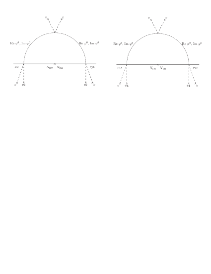
Figure 1: Loop Feynman diagrams contributing to the entries of the neutrino mass matrix. Here $i,j=1,2,3$. The cross marks in the internal lines with $N_{nR}-N_{nR}$ ($n=1,2$) denote the insertion of the mass $m_{N_{nR}}$.

Considering these diagrams and the Dirac couplings in Eq.(12) with $\varphi$, which we represent in the matrix form $Y^{\nu}_{\varphi}$:

$$Y^{\nu}_{\varphi}=\frac{v}{\sqrt{2}\Lambda^{2}}\left(\begin{array}[]{cc}v_{\Phi}y^{(\nu)}_{1}&v_{\Xi}y^{(\nu)}_{2}\\ 0&v_{\Xi}y^{(\nu)}_{2}\\ 0&v_{\Xi}y^{(\nu)}_{2}\end{array}\right),$$ (14)

one reads off there will be a democratic contribution associated with the $y^{(\nu)}_{2}$ coupling filling each entry in $M_{\nu}$ equally (due to the coupling to the combination $\left(\overline{l}_{1L}+\overline{l}_{2L}+\overline{l}_{3L}\right)$) whereas the $y^{(\nu)}_{1}$ coupling is responsible for a contribution solely to the $11$ entry of $M_{\nu}$. Thus we write the effective neutrino mass matrix in the form

$$M_{\nu}=\left(\begin{array}[]{ccc}A_{1}^{\left(\nu\right)}&A_{2}^{\left(\nu\right)}&A_{2}^{\left(\nu\right)}\\ A_{2}^{\left(\nu\right)}&A_{2}^{\left(\nu\right)}&A_{2}^{\left(\nu\right)}\\ A_{2}^{\left(\nu\right)}&A_{2}^{\left(\nu\right)}&A_{2}^{\left(\nu\right)}\end{array}\right),$$ (15)

where the dimensionful parameters $A_{1}^{\left(\nu\right)}$ and $A_{2}^{\left(\nu\right)}$ follow from the loop functions of the diagrams in Fig. 1.

$$A_{1}^{\left(\nu\right)} \simeq \frac{\left(y_{2}^{\left(\nu\right)}\right)^{2}v_{\Xi}^{2}v^{2}m_{N_{2R}}}{32\pi^{2}\Lambda^{4}}f\left(m_{\mathop{\mathrm{R}e}\varphi},m_{\mathop{\mathrm{I}m}\varphi},m_{N_{2R}}\right)$$ (16)

$$\qquad+\frac{\left(y_{1}^{\left(\nu\right)}\right)^{2}v_{\Phi}^{2}v^{2}m_{N_{1R}}}{32\pi^{2}\Lambda^{4}}f\left(m_{\mathop{\mathrm{R}e}\varphi},m_{\mathop{\mathrm{I}m}\varphi},m_{N_{1R}}\right),$$

$$A_{2}^{\left(\nu\right)}\simeq\frac{\left(y_{2}^{\left(\nu\right)}\right)^{2}v_{\Xi}^{2}v^{2}m_{N_{2R}}}{32\pi^{2}\Lambda^{4}}f\left(m_{\mathop{\mathrm{R}e}\varphi},m_{\mathop{\mathrm{I}m}\varphi},m_{N_{2R}}\right),$$ (17)

$$f\left(m_{\mathop{\mathrm{R}e}\varphi},m_{\mathop{\mathrm{I}m}\varphi},m_{N_{kR}}\right)=\frac{m_{\mathop{\mathrm{R}e}\varphi}^{2}}{m_{\mathop{\mathrm{R}e}\varphi}^{2}-m_{N_{kR}}^{2}}\ln\left(\frac{m_{\mathop{\mathrm{R}e}\varphi}^{2}}{m_{N_{kR}}^{2}}\right)-\frac{m_{\mathop{\mathrm{I}m}\varphi}^{2}}{m_{\mathop{\mathrm{I}m}\varphi}^{2}-m_{N_{kR}}^{2}}\ln\left(\frac{m_{\mathop{\mathrm{I}m}\varphi}^{2}}{m_{N_{kR}}^{2}}\right)\,,$$ (18)

with $k=1$, $2$. We note that $\varphi$ needs to be a complex scalar otherwise the loop functions vanish, and further the real and imaginary parts of $\varphi$ must not have degenerate masses. The structure of $M_{\nu}$ is such that it has an eigenvector $(0,1,-1)/\sqrt{2}$ with a vanishing eigenvalue, corresponding therefore to a massless neutrino. This means the neutrino sector’s contribution to the PMNS matrix, $U^{\left(\nu\right)}$, has one direction which is $(0,1,-1)/\sqrt{2}$, meaning $\theta_{13}^{\left(\nu\right)}=0$ and $\theta_{23}^{\left(\nu\right)}=\pi/4$. This gets modified by the contribution from the charged lepton sector such that the reactor angle is non-zero, but given that the associated state is the massless state this structure is viable for the inverted hierarchy of neutrino masses (but not for the normal hierarchy). Indeed, we find that for our model the normal hierarchy scenario leads to a too large reactor mixing angle, thus being ruled out by the current data on neutrino oscillation experiments.

The $\mathcal{O}(1)$ dimensionless couplings $a_{i}^{\left(l\right)}$ ($i=1,\cdots,4$) determine the charged lepton masses, the reactor mixing parameter $\sin^{2}\theta_{13}\neq 0$ and the deviation $\sin^{2}\theta_{23}-1/2\neq 0$, which are correlated:

$$\sin^{2}\theta_{23}=\frac{1}{2\,(1-\sin^{2}\theta_{13})}\,.$$ (19)

In turn, $A_{1}^{\left(\nu\right)}$ and $A_{2}^{\left(\nu\right)}$ are dimensionful parameters crucial to determine the neutrino mass squared splittings as well as the solar angle $\sin^{2}\theta_{12}$. For the sake of simplicity and proving these leptonic structures are viable, we assume that the parameters $a_{l}^{\left(l\right)}$ ($l=1,\cdots,4$), $A_{2}^{\left(\nu\right)}$ are real whereas $A_{1}^{\left(\nu\right)}$ is taken to be complex. We have checked numerically that the simplest scenario of all lepton parameters ($a_{l}^{\left(l\right)}$ ($l=1,\cdots,4$), $A_{1}^{\left(\nu\right)}$and $A_{2}^{\left(\nu\right)}$) being real leads to a solar mixing parameter $\sin^{2}\theta_{12}$ close to about $0.2$, which is below its $3\sigma$ experimental lower bound.

In order to reproduce the experimental values of the physical observables of the lepton sector, i.e. the three charged lepton masses, two neutrino mass squared splittings and the three leptonic mixing parameters, we proceed to fit the parameters $a_{k}^{\left(l\right)}$ ($k=1,\cdots,4$), $\left|A_{1}^{\left(\nu\right)}\right|$,$\ A_{2}^{\left(\nu\right)}$ and $\arg\left[A_{1}^{\left(\nu\right)}\right]$.

For the case of inverted neutrino mass hierarchy we find the following best fit result

$$a_{1}^{\left(l\right)} \simeq 1.936,\hskip 28.45274pta_{2}^{\left(l\right)}\simeq 1.025,\hskip 28.45274pta_{3}^{\left(l\right)}\simeq 0.864,\hskip 28.45274pta_{4}^{\left(l\right)}\simeq 0.813,$$

$$\left|A_{1}^{\left(\nu\right)}\right| \simeq 69.7\hskip 1.42262pt\mbox{meV},\hskip 28.45274ptA_{2}^{\left(\nu\right)}\simeq 20.6\hskip 1.42262pt\mbox{meV},\hskip 28.45274pt\arg\left[A_{1}^{\left(\nu\right)}\right]\simeq-58.26^{\circ}.$$ (20)

The small hierarchy between effective parameters $\left|A_{1}^{\left(\nu\right)}\right|$,$\ A_{2}^{\left(\nu\right)}$ is consistent with the mild hierarchy between $\langle\Phi\rangle$ and $\langle\Xi\rangle$.

As follows from Eqs. (16)-(18), the obtained numerical values given above for the neutrino parameters $\left|A_{1}^{\left(\nu\right)}\right|$, $A_{2}^{\left(\nu\right)}$ and $\arg\left[A_{1}^{\left(\nu\right)}\right]$ can be obtained from the following benchmark point:

$$m_{N_{1}} = 500\hskip 1.42262pt\mbox{GeV},\hskip 14.22636ptm_{N_{2}}=2\hskip 1.42262pt\hskip 1.42262pt\mbox{TeV},\hskip 14.22636ptm_{\mathop{\mathrm{R}e}\varphi}=900\hskip 1.42262pt\hskip 1.42262pt\mbox{GeV},\hskip 14.22636ptm_{\mathop{\mathrm{I}m}\varphi}=600\hskip 1.42262pt\mbox{GeV},$$

$$\Lambda = 2.41\times 10^{5}\leavevmode\nobreak\ \mbox{TeV},\hskip 14.22636pt\left|y_{1\nu}\right|=1.12,\hskip 14.22636pty_{2\nu}=0.61,\hskip 14.22636pt\arg\left[y_{1\nu}\right]\simeq-37.4^{\circ}\,.$$ (21)

Observable	Model value	Experimental value
		$1\sigma$ range	$2\sigma$ range	$3\sigma$ range
$m_{e}$ [MeV]	$0.487$	$0.487$	$0.487$	$0.487$
$m_{\mu}$ [MeV]	$102.8$	$102.8\pm 0.0003$	$102.8\pm 0.0006$	$102.8\pm 0.0009$
$m_{\tau}$ [GeV]	$1.75$	$1.75\pm 0.0003$	$1.75\pm 0.0006$	$1.75\pm 0.0009$
$\Delta m_{21}^{2}$ [$10^{-5}$eV2] (IH)	$7.56$	$7.56\pm 0.19$	$7.20-7.95$	$7.05-8.14$
$\Delta m_{13}^{2}$ [$10^{-3}$eV2] (IH)	$2.49$	$2.49\pm 0.04$	$2.41-2.57$	$2.37-2.61$
$\delta$ [∘] (IH)	$281.6$	$259_{-41}^{+47}$	$182-347$	$0-31$
				$142-360$
$\sin^{2}\theta_{12}$ (IH)	$0.321$	$0.321_{-0.016}^{+0.018}$	$0.289-0.359$	$0.273-0.379$
$\sin^{2}\theta_{23}$ (IH)	$0.511$	$0.596_{-0.018}^{+0.017}$	$0.404-0.456$	$0.388-0.638$
			$0.556-0.625$
$\sin^{2}\theta_{13}$ (IH)	$0.0214$	$0.0214_{-0.00085}^{+0.00082}$	$0.0197-0.0230$	$0.0189-0.0239$

Table 4: Model and experimental values of the charged lepton masses, neutrino mass squared splittings and leptonic mixing parameters for the inverted (IH) mass hierarchy. The model values for CP violating phase are also shown. The experimental values of the charged lepton masses are taken from Ref. Bora:2012tx , whereas the range for experimental values of neutrino mass squared splittings and leptonic mixing parameters, are taken from Ref. deSalas:2017kay .

The benchmark point given above is one out of the many similar solutions that yields physical observables for the neutrino sector consistent with the experimental data. We have numerically checked that for a fixed mass splittings between the masses of the real and imaginary components of $\varphi$, the cutoff scale has a low sensitivity with the masses of the scalar and fermionic seesaw mediators. In addition, we have checked that lowering the mass splitting between $Re\varphi$ and $Im\varphi$ leads to a decrease of the cutoff scale. In particular lowering this mass splitting from $50\%$ up to $0.1\%$ of the mass of $Im\varphi$ leads to a decrease of the cutoff scale from $\sim 10^{8}$ GeV up to $\sim 10^{7}$ GeV. From Table 4, it follows that the reactor $\sin^{2}\theta_{13}$ and solar $\sin^{2}\theta_{12}$ leptonic mixing parameters are in excellent agreement with the experimental data, whereas the atmospheric $\sin^{2}\theta_{23}$ mixing parameter is deviated $3\sigma$ away from its best fit value. Fig. 2 shows the correlation between the solar mixing parameter $\sin^{2}\theta_{12}$ and the Jarlskog invariant for the case of inverted neutrino mass hierarchy. We found a leptonic Dirac CP violating phase of $281.6^{\circ}$ and a Jarlskog invariant close to about $-3.3\times 10^{-2}$ for the inverted neutrino mass hierarchy.

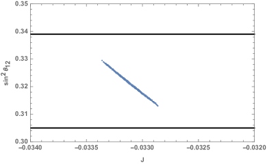
Figure 2: Correlation between the solar mixing parameter $\sin^{2}\theta_{12}$ and the Jarlskog invariant for the case of inverted neutrino mass hierarchy. The horizontal lines are the minimum and maximum values of the solar mixing parameter $\sin^{2}\theta_{12}$ inside the $1\sigma$ experimentally allowed range.

Let us consider the effective Majorana neutrino mass parameter

$$m_{ee}=\left|\sum_{j}U_{ek}^{2}m_{\nu_{k}}\right|,$$ (22)

where $U_{ej}$ and $m_{\nu_{k}}$ are the PMNS leptonic mixing matrix elements and the neutrino Majorana masses, respectively. The neutrinoless double beta ($0\nu\beta\beta$) decay amplitude is proportional to $m_{ee}$. From Eq. (15) it follows that in our model there is a massless neutrino. It is well known that in this case, independently of the other parameters, one expects for the inverted neutrino mass hierarchy 15 meV $<m_{ee}<$ 50 meV. With the model best fit values in Table 4 we find

$$m_{ee}\simeq 41.3\leavevmode\nobreak\ \mbox{meV}\,.$$ (23)

This is within the declared reach of the next-generation bolometric CUORE experiment Alessandria:2011rc or, more realistically, of the next-to-next-generation ton-scale $0\nu\beta\beta$-decay experiments. The current most stringent experimental upper limit $m_{ee}\leq 160$ meV is set by $T_{1/2}^{0\nu\beta\beta}(^{136}\mathrm{Xe})\geq 1.1\times 10^{26}$ yr at 90% C.L. from the KamLAND-Zen experiment KamLAND-Zen:2016pfg .

In theory, Lepton Flavour Violation processes are expected from this kind of model. However, in realisations such as these the new scale $\Lambda$ associated with family symmetry breaking scale is very high. Thus, the rate of muon conversion processes such as $\mu N\to eN$ ($N$ is nucleon), $\mu\to eee$, $\mu\to e\gamma$ is several orders of magnitude beyond experimental reach Varzielas:2010mp .

5 Scalar Potential

In this section we consider the scalar potential. As can be seen in Table 1, the scalar content of the model has many degrees of freedom. We assume that all scalars except for $\phi$ and $\varphi$ get their VEVs at the family symmetry breaking scale, which should be near the cutoff scale $\Lambda$, much greater than the electroweak breaking scale defined by the VEV of $\langle\phi\rangle\sim v$ (we can check the self-consistency of this assumption in the benchmark point in Eq. (21)). Due to this, the family symmetry breaking scalars decouple, such that we have at the TeV scale the effective potential $V(\phi,\varphi)$. We divide it into separate parts for convenience, and use without loss of generality the mass eigenstates $\mathop{\mathrm{R}e}\varphi$, $\mathop{\mathrm{I}m}\varphi$ instead of $\varphi$, $\varphi^{*}$:

$$V(\phi,\varphi)=V(\phi)+V(\phi,\varphi)+V(\varphi)$$ (24)

where

$$V(\phi)=-\mu^{2}\left(\phi^{\dagger}\cdot\phi\right)+\lambda\left(\phi^{\dagger}\cdot\phi\right)^{2}+h.c,$$ (25)

is simply the SM potential (one Higgs doublet) and

$$V(\phi,\varphi)=\gamma_{1}\left(\phi^{\dagger}\cdot\phi\right)\mathop{\mathrm{R}e}\varphi^{2}+\gamma_{2}\left(\phi^{\dagger}\cdot\phi\right)\mathop{\mathrm{I}m}\varphi^{2}+h.c,$$ (26)

has only quartic interactions between the doublet $\phi$ and the $\mathbb{Z}_{2}$-odd scalar $\varphi$. The term

$$V(\varphi)=-m_{1}^{2}\mathop{\mathrm{R}e}\varphi^{2}-m_{2}^{2}\mathop{\mathrm{I}m}\varphi^{2}+\lambda_{1}\left(\mathop{\mathrm{R}e}\varphi\right)^{4}+\lambda_{2}\left(\mathop{\mathrm{I}m}\varphi\right)^{4}+\lambda_{3}\left(\mathop{\mathrm{R}e}\varphi^{2}\mathop{\mathrm{I}m}\varphi^{2}\right)+h.c,$$ (27)

has the masses and quartic interactions that involve only the $\mathbb{Z}_{2}$ odd scalar. Given this, the masses of the real and imaginary parts of $\varphi$ will not be degenerate. As the symmetry is enhanced in the limit of degeneracy (a $U(1)$ symmetry instead of the preserved $\mathbb{Z}_{2}$), if the splitting between their masses is small it remains small, and a small splitting is technically natural in that sense as it is protected by an approximate symmetry.

6 Dark Matter Constraints

In this section we consider the possibilities offered by the model to provide a viable DM candidate. The $\mathbb{Z}_{2}$ symmetry, under which only the scalar field $\varphi$ and the fermions $N_{1R}$ and $N_{2R}$ are charged, remains unbroken and stabilizes the lightest $\mathbb{Z}_{2}$-odd mass eigenstate.

6.1 Scalar Dark Matter Scenario

The first scenario considered is the one where one component of the scalar field $\varphi$ is the lightest $\mathbb{Z}_{2}$-odd particle. In this case, DM is produced in the early Universe via the vanilla WIMP paradigm. If Im $\varphi$ is the lightest $\mathbb{Z}_{2}$ odd state, it can annihilate into a pair of SM particles via the $s$-channel exchange of a Higgs boson. Additionally, the annihilation into Higgs bosons also occurs via the contact interaction and the mediation by an Im $\varphi$ in the $t$- and $u$-channels. Finally, DM could also annihilate into a pair SM neutrino/antineutrino via the $t$- and $u$-channel exchange of a $N_{1}$. However the latter channel is typically very suppressed by the tiny effective neutrino Yukawa coupling $y_{1\chi}\ll 1$. Hence, the DM relic abundance is mainly governed by the DM mass $m_{\text{Im}\leavevmode\nobreak\ \varphi}$ and the quartic coupling $\gamma_{2}$, between two DM particles and two Higgs bosons. The freeze-out of heavy DM particles ($m_{\text{Im}\leavevmode\nobreak\ \varphi}>m_{h}$) is largely dominated by the annihilations into Higgs bosons, with a thermally-averaged cross-section given by:

$$\langle\sigma v\rangle\simeq\frac{\gamma_{2}^{2}}{32\pi}\,\left[\frac{\gamma_{2}\,v^{2}\,\left(m_{h}^{2}-4\,m_{\text{Im}\leavevmode\nobreak\ \varphi}^{2}\right)+m_{h}^{4}-4\,m_{\text{Im}\leavevmode\nobreak\ \varphi}^{4}}{m_{\text{Im}\leavevmode\nobreak\ \varphi}\,\left(m_{h}^{4}-6\,m_{h}^{2}\,m_{\text{Im}\leavevmode\nobreak\ \varphi}^{2}+8\,m_{\text{Im}\leavevmode\nobreak\ \varphi}^{4}\right)}\right]^{2}\,.$$ (28)

In Fig. 3 it is shown the parameter space ($\gamma_{2},\,m_{\text{Im}\leavevmode\nobreak\ \varphi}$) giving rise to the observed DM relic abundance. The black thick line corresponds to the full computation using micrOMEGAs Belanger:2006is ; Belanger:2008sj ; Belanger:2010pz ; Belanger:2013oya , whereas the red line to the analytical case given by Eq. (28). The vertical dashed blue line corresponds to $m_{\text{Im}\leavevmode\nobreak\ \varphi}=m_{h}$. The direct detection constraints are obtained by comparing the spin-independent cross section for the scattering of the DM off of a nucleon,

$$\sigma_{\text{SI}}=\frac{\gamma_{2}^{2}\,m_{N}^{4}\,f^{2}}{8\pi\,m_{h}^{4}\,m_{\text{Im}\leavevmode\nobreak\ \varphi}^{2}}\,,$$ (29)

to the latest limits on $\sigma_{\text{SI}}$ provided by PandaX-II Cui:2017nnn . Here $m_{N}$ is the nucleon mass and $f\simeq 1/3$ corresponds to the form factor Farina:2009ez ; Giedt:2009mr . Again, the analytical result is in good agreement with the numerical computation by micrOMEGAs. Fig. 3 also presents the DM spin-independent direct detection exclusion region, that sets strong tension for the model if the DM is lighter than $\sim 400$ GeV.

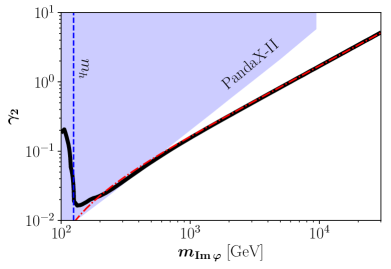
Figure 3: Scalar Dark Matter Scenario. Parameter space generating the observed DM relic abundance via the WIMP mechanism, using the full annihilation cross-section (thick black line) and the only the annihilation into Higgs bosons (thin red line). The light blue region is in tension with the latest PandaX-II results.

6.2 Fermionic Dark Matter Scenario

The second case corresponds to the scenario where $N_{1R}$ is the lightest $\mathbb{Z}_{2}$-odd particle. DM can annihilate into a pair of SM neutrinos via the $t$-channel exchange of the real and the imaginary parts of $\varphi$. This comes from an effective neutrino Yukawa coupling $y_{1\chi}\equiv\left|y_{1\nu}\right|\,\lambda\,\frac{v}{\Lambda}$ produced by Eq. (5) or its expanded version, Eq. (12):

$$\mathcal{L}\supset y_{1}^{\left(\nu\right)}\,\lambda\,\overline{l}_{1L}\,N_{1R}\,\varphi\frac{\langle\widetilde{\phi\rangle}}{\Lambda}\,.$$ (30)

The DM relic abundance is then governed by the DM mass $m_{N_{1}}$, the mediator masses $m_{\text{Re}\,\varphi}$ and $m_{\text{Im}\,\varphi}$, and the effective Yukawa coupling $y_{1\chi}$. The thermally-averaged annihilation cross-section is given by:

$$\langle\sigma v\rangle\simeq\frac{9\,y_{1\chi}^{4}}{32\pi}\,\frac{m_{N_{1}}^{2}\,\left(2m_{N_{1}}^{2}+m_{\text{Re}\,\varphi}^{2}+m_{\text{Im}\,\varphi}^{2}\right)^{2}}{\left(m_{N_{1}}^{2}+m_{\text{Re}\,\varphi}^{2}\right)^{2}\,\left(m_{N_{1}}^{2}+m_{\text{Im}\,\varphi}^{2}\right)^{2}}\,.$$ (31)

Fig. 4 shows the required effective coupling $y_{1\chi}$ in order to reproduce the observed DM relic abundance via the standard thermal WIMP paradigm, and assuming $m_{\text{Re}\,\varphi}=m_{\text{Im}\,\varphi}$.

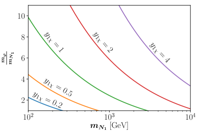
Figure 4: Fermionic Dark Matter Scenario. Effective coupling $y_{1\chi}$ needed in order to generate the observed relic abundance via the WIMP mechanism, assuming $m_{\varphi}\equiv m_{\text{Re}\,\varphi}\sim m_{\text{Im}\,\varphi}$.

As expected for WIMP DM, the effective coupling has to be of the order of $\mathcal{O}(1)$, if DM is heavier than $\sim 100$ GeV. For the DM production this is perfectly viable, however we also want to generate the neutrino masses. In what follows we proceed to scan for the CP odd scalar mass $m_{Im\varphi}$ and effective neutrino Yukawa coupling $y_{1\chi}=\left|y_{1\nu}\right|\,\lambda\,\frac{v}{\Lambda}$ needed required to reproduce the values of the neutrino parameters $\left|A_{1}^{\left(\nu\right)}\right|$, $A_{2}^{\left(\nu\right)}$ and $\arg\left[A_{1}^{\left(\nu\right)}\right]$ shown in Eq. (20). Fixing the right handed Majorana neutrino masses to typical values $m_{N_{1}}\sim 500$ GeV, $m_{N_{2}}\sim 2$ TeV, $m_{\text{Im}\varphi}\sim 1$ TeV and $\Lambda\sim 10^{8}$ GeV, required to reproduce the values of the neutrino parameters $\left|A_{1}^{\left(\nu\right)}\right|$, $A_{2}^{\left(\nu\right)}$ and $\arg\left[A_{1}^{\left(\nu\right)}\right]$, the effective neutrino Yukawa coupling $y_{1\chi}$ has to be of the order of $10^{-7}$ to $10^{-4}$. Values in this ballpark are too small to reproduce the observed DM relic abundance via the WIMP mechanism, which requires $\mathcal{O}(1)$ effective Yukawa coupling $y_{1\chi}$ as indicated by Fig. 4. Consequently the fermionic DM scenario of our model can not be produced via the usual WIMP paradigm.

Alternatively, very suppressed couplings between the visible and the dark sectors are characteristic in non-thermal scenarios where the DM relic abundance is created in the early Universe via freeze-in McDonald:2001vt ; Choi:2005vq ; Kusenko:2006rh ; Petraki:2007gq ; Hall:2009bx ; Bernal:2017kxu . Fig. 5 shows the effective couplings required in order to produce FIMP DM. As expected for this kind of scenarios, $y_{1\chi}$ is in the range $\sim 10^{-8}$ to $\sim 10^{-11}$. The light blue region is disregarded because $N_{1}$ is not the lightest particle of the dark sector.

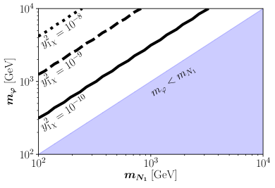
Figure 5: Fermionic Dark Matter Scenario. Effective coupling $y_{1\chi}^{2}$ needed in order to generate the observed relic abundance via the FIMP mechanism, assuming $m_{\varphi}\equiv m_{\text{Re}\,\varphi}\sim m_{\text{Im}\,\varphi}$.

Finally, to close this section, we discuss the splitting between the masses of the real and imaginary parts of $\varphi$. To start, we note that a small scalar mass splitting of $10^{-3}$ times the mass of the imaginary part of $\varphi$ (which is required in order to have fermionic DM through the FIMP mechanism) may look unnatural, but it is actually technically natural in the sense that it is protected by a symmetry: in the limit where the RH neutrino masses and the splitting of the $\varphi$ masses vanish, the symmetry of the Lagrangian is enlarged from the $\mathbb{Z}_{2}$ to a $U(1)$ symmetry. The non-trivial $U(1)$ charges of the RH neutrinos and of $\varphi$ under this $U(1)$ would forbid Majorana terms for the RH neutrinos and force the masses of the real and imaginary parts of $\varphi$ to be the same. Considering this, if the $U(1)$ is broken only by the Majorana terms (but not in the scalar potential), the splitting of the masses is no longer protected by the symmetry and is generated, but only radiatively. In such a scenario, the splitting would be naturally small.

Although we do not consider this scenario in great detail, we propose also some more explicit mechanisms that can explain the splitting between the masses of the real and imaginary parts of $\varphi$ when starting from the symmetry limit where the splitting vanishes. The first possibility consists in extending our model by adding an extra spontaneously broken $\mathbb{Z}_{3}$ discrete symmetry under which $\varphi$ is assumed to have a charge $+1$ (in additive notation). In addition, an extra SM scalar singlet, i.e. $\zeta$ , with $\mathbb{Z}_{3}$ charge +1 has to be added. The remaining scalar and fermions are neutral under $\mathbb{Z}_{3}$. Consequently no new contributions to the quarks, charged leptons and neutrino Yukawa terms originate from the extra field $\zeta$ and the $\mathbb{Z}_{3}$ discrete symmetry. The splitting between the masses of $\mathop{\mathrm{R}e}\varphi$ and $\mathop{\mathrm{I}m}\varphi$ will arise from the trilinear scalar interaction $A\varphi^{2}\zeta$ which preserves both this added $\mathbb{Z}_{3}$ and the existing $\mathbb{Z}_{2}$. The invariance of the neutrino Yukawa interactions under the $\mathbb{Z}_{3}$ discrete symmetry requires that the right handed Majorana neutrinos $N_{1R}$ and $N_{2R}$ should have a $\mathbb{Z}_{3}$ charge equal to $+1$, such that their masses will need to arise from the Yukawa interactions $\overline{N}_{1R}N_{1R}^{C}\zeta$ and $\overline{N}_{2R}N_{2R}^{C}\zeta$ after the spontaneous breaking of the $\mathbb{Z}_{3}$ discrete group. This is an explicit realization of the mechanism described above, showing there is a relation between the $\varphi$ mass splitting and the $N_{iR}$ masses. If this $\mathbb{Z}_{3}$ is broken at the TeV scale the right handed Majorana neutrinos are within the LHC reach and there is a viable fermionic DM candidate through the FIMP mechanism.

A different mechanism to generate the splitting by replacing the SM scalar singlet $\varphi$ with an inert $SU(2)$ scalar doublet charged under the preserved $\mathbb{Z}_{2}$ symmetry. That scenario was proposed for the first time in Ref. Ma:2006km . In that scenario, the splitting between the masses of $\mathop{\mathrm{R}e}\varphi$ and $\mathop{\mathrm{I}m}\varphi$ (in that scenario $\varphi$ is a $SU(2)$ scalar doublet) will arise form the quartic scalar interaction $\left(\phi^{\dagger}\cdot\varphi\right)^{2}$, as explained in detail in Ref. Ma:2006km . In this case, the coupling between right-handed neutrinos and $\varphi$ does not include the Higgs $\phi$.

7 Conclusions

We have built a viable family symmetry model based on the $\Delta\left(27\right)\times\mathbb{Z}_{2}\times\mathbb{Z}_{5}\times\mathbb{Z}_{6}\times\mathbb{Z}_{10}\times\mathbb{Z}_{16}$ discrete group, which leads to a mixing inspired texture for the quarks and to similarly predictive structures for the leptons. For the quarks, the down sector parameters control the Cabibbo angle, and the up and down sector parameters control the remaining angles. For the leptons, the effective neutrino parameters that arise after radiative seesaw control the solar angle, and the charged lepton parameters control the reactor angle, which is also correlated to the deviation of the atmospheric angle from its maximal value. The model is only viable for inverted hierarchy and after fitting to the best-fit values of the solar and reactor angle, predicts $\sin^{2}\theta_{23}\simeq 0.51$, $\delta\simeq 281.6^{\circ}$ and $m_{ee}=41.3$ meV.

Additionally, the model has viable DM candidates, stabilized by an unbroken $\mathbb{Z}_{2}$ symmetry, which we analyze quantitatively. A simple possibility is that there is scalar WIMP DM, which is produced through the Higgs portal. An alternative scenario is when we consider fermionic DM, which in our model would be the lightest right-handed neutrino. In order for it to be a WIMP and to obtain the right abundance, its effective coupling to the visible sector is too large to be consistent with what is required by the effective neutrino masses. Instead, if our fermionic DM candidate is a FIMP, the effective coupling needs to be quite small. This is consistent with obtaining the required neutrino masses but requires a very small splitting of the real and imaginary components of the $\mathbb{Z}_{2}$-odd scalar (the splitting divided by the mass scale would be at the per mille level). The smallness of the splitting is technically natural as when the splitting goes to zero, the symmetry of the theory is enhanced.

This model addresses the flavour problem while providing a viable DM candidate (scalar or fermionic), and is a novel example of the interplay of constraints coming from the observed DM abundance to a family symmetry model, namely by relating the DM abundance to the light neutrino masses.

Appendix A The Product Rules of the $\boldsymbol{\Delta(27)}$ Discrete Group

The $\Delta(27)$ discrete group is a subgroup of $SU(3)$, has 27 elements divided into 11 conjugacy classes. Then the $\Delta(27)$ discrete group contains the following 11 irreducible representations: two triplets, i.e. $\mathbf{3}_{[0][1]}$ (which we denote by $\mathbf{3}$) and its conjugate $\mathbf{3}_{[0][2]}$ (which we denote by $\overline{\mathbf{3}}$) and 9 singlets, i.e. $\mathbf{1}_{k,l}$ ($k,l=0,1,2$), where $k$ and $l$ correspond to the $\mathbb{Z}_{3}$ and $\mathbb{Z}_{3}^{\prime}$ charges, respectively Ishimori:2010au . The $\Delta(27)$ discrete group, which is a simple group of the type $\Delta(3n^{2})$ with $n=3$, is isomorphic to the semi-direct product group $(\mathbb{Z}_{3}^{\prime}\times\mathbb{Z}_{3}^{\prime\prime})\rtimes\mathbb{Z}_{3}$ Ishimori:2010au . It is worth mentioning that the simplest group of the type $\Delta(3n^{2})$ is $\Delta(3)\equiv\mathbb{Z}_{3}$. The next group is $\Delta(12)$, which is isomorphic to $A_{4}$. Consequently the $\Delta(27)$ discrete group is the simplest nontrivial group of the type $\Delta(3n^{2})$. Any element of the $\Delta(27)$ discrete group can be expressed as $b^{k}a^{m}{a^{\prime}}^{n}$, being $b$, $a$ and $a^{\prime}$ the generators of the $\mathbb{Z}_{3}$, $\mathbb{Z}_{3}^{\prime}$ and $\mathbb{Z}_{3}^{\prime\prime}$ cyclic groups, respectively. These generators fulfill the relations:

$$a^{3}=a^{\prime 3}=b^{3}=1,\hskip 14.22636ptaa^{\prime}=a^{\prime}a,$$

$$bab^{-1}=a^{-1}a^{\prime-1},\,\,ba^{\prime}b^{-1}=a.$$ (32)

The characters of the $\Delta(27)$ discrete group are shown in Table 5. Here $n$ is the number of elements, $h$ is the order of each element, and $\omega=e^{\frac{2\pi i}{3}}=-\frac{1}{2}+i\frac{\sqrt{3}}{2}$ is the cube root of unity, which satisfies the relations $1+\omega+\omega^{2}=0$ and $\omega^{3}=1$. The conjugacy classes of $\Delta(27)$ are given by:

$$\begin{array}[]{ccc}C_{1}:&\{e\},&h=1,\\ C_{1}^{(1)}:&\{a,a^{\prime 2}\},&h=3,\\ C_{1}^{(2)}:&\{a^{2},a^{\prime}\},&h=3,\\ C_{3}^{(0,1)}:&\{a^{\prime 2}a^{\prime 2}\},&h=3,\\ C_{3}^{(0,2)}:&\{a^{\prime 2},a^{2},aa^{\prime}\},&h=3,\\ C_{3}^{(1,p)}:&\{ba^{p},ba^{p-1}a^{\prime p-2}a^{\prime 2}\},&h=3,\\ C_{3}^{(2,p)}:&\{ba^{p},ba^{p-1}a^{\prime p-2}a^{\prime 2}\},&h=3.\\ &&\end{array}$$

	h	$\chi_{1_{(r,s)}}$	$\chi_{3_{[0,1]}}$	$\chi_{3_{[0,2]}}$
$1C_{1}$	1	1	3	3
$1C_{1}^{(1)}$	1	1	$3\omega^{2}$	$3\omega$
$1C_{1}^{(2)}$	1	1	$3\omega$	$3\omega^{2}$
$3C_{1}^{(0,1)}$	$3$	$\omega^{s}$	$0$	$0$
$3C_{1}^{(0,2)}$	$3$	$\omega^{2s}$	$0$	$0$
$C_{3}^{(1,p)}$	$3$	$\omega^{r+sp}$	0	0
$C_{3}^{(2,p)}$	$3$	$\omega^{2r+sp}$	0	0

Table 5: Characters of $\Delta(27)$.

The tensor products between $\Delta(27)$ triplets are described by the following relations Ishimori:2010au :

$$\vspace{-1cm}\begin{pmatrix}x_{1,-1}\\ x_{0,1}\\ x_{-1,0}\\ \end{pmatrix}_{\mathbf{3}_{[0][1]}}\otimes\begin{pmatrix}y_{1,-1}\\ y_{0,1}\\ y_{-1,0}\\ \end{pmatrix}_{\mathbf{3}_{[0][1]}} = \begin{pmatrix}x_{1,-1}y_{1,-1}\\ x_{0,1}y_{0,1}\\ x_{-1,0}y_{-1,0}\\ \end{pmatrix}_{\mathbf{3}_{[0][2]}^{\left(S_{1}\right)}}\oplus\frac{1}{2}\begin{pmatrix}x_{0,1}y_{-1,0}+x_{-1,0}y_{0,1}\\ x_{-1,0}y_{1,-1}+x_{1,-1}y_{-1,0}\\ x_{1,-1}y_{0,1}+x_{0,1}y_{1,-1}\\ \end{pmatrix}_{\mathbf{3}_{[0][2]}^{\left(S_{2}\right)}}$$ (33)

$$\oplus\frac{1}{2}\begin{pmatrix}x_{0,1}y_{-1,0}-x_{-1,0}y_{0,1}\\ x_{-1,0}y_{1,-1}-x_{1,-1}y_{-1,0}\\ x_{1,-1}y_{0,1}-x_{0,1}y_{1,-1}\\ \end{pmatrix}_{\mathbf{3}_{[0][2]}^{\left(A\right)}},$$

$$\begin{pmatrix}x_{2,-2}\\ x_{0,2}\\ x_{-2,0}\\ \end{pmatrix}_{\mathbf{3}_{[0][2]}}\otimes\begin{pmatrix}y_{2,-2}\\ y_{0,2}\\ y_{-2,0}\\ \end{pmatrix}_{\mathbf{3}_{[0][2]}} = \begin{pmatrix}x_{2,-2}y_{2,-2}\\ x_{0,2}y_{0,2}\\ x_{-2,0}y_{-2,0}\\ \end{pmatrix}_{\mathbf{3}_{[0][1]}^{\left(S_{1}\right)}}\oplus\frac{1}{2}\begin{pmatrix}x_{0,2}y_{-2,0}+x_{-2,0}y_{0,2}\\ x_{-2,0}y_{2,-2}+x_{2,-2}y_{-2,0}\\ x_{2,-2}y_{0,2}+x_{0,2}y_{2,-2}\\ \end{pmatrix}_{\mathbf{3}_{[0][1]}^{\left(S_{2}\right)}}$$ (34)

$$\oplus\frac{1}{2}\begin{pmatrix}x_{0,2}y_{-2,0}-x_{-2,0}y_{0,2}\\ x_{-2,0}y_{2,-2}-x_{2,-2}y_{-2,0}\\ x_{2,-2}y_{0,2}-x_{0,2}y_{2,-2}\\ \end{pmatrix}_{\mathbf{3}_{[0][1]}^{\left(A\right)}},$$

$$\begin{pmatrix}x_{1,-1}\\ x_{0,1}\\ x_{-1,0}\\ \end{pmatrix}_{\mathbf{3}_{[0][1]}}\otimes\begin{pmatrix}y_{-1,1}\\ y_{0,-1}\\ y_{1,0}\\ \end{pmatrix}_{\mathbf{3}_{[0][2]}} = \sum_{r}(x_{1,-1}y_{-1,1}+\omega^{2r}x_{0,1}y_{0,-1}+\omega^{r}x_{-1,0}y_{1,0})_{\mathbf{1}_{(r,0)}}$$

$$\oplus \sum_{r}(x_{1,-1}y_{0,-1}+\omega^{2r}x_{0,1}y_{1,0}+\omega^{r}x_{-1,0}y_{-1,1})_{\mathbf{1}_{(r,1)}}$$

$$\oplus \sum_{r}(x_{1,-1}y_{1,0}+\omega^{2r}x_{0,1}y_{-1,1}+\omega^{r}x_{-1,0}y_{0,-1})_{\mathbf{1}_{(r,2)}}.$$

The multiplication rules between $\Delta(27)$ singlets and $\Delta(27)$ triplets are given by Ishimori:2010au :

$$\begin{pmatrix}x_{(1,-1)}\\ x_{(0,1)}\\ x_{(-1,0)}\end{pmatrix}_{\mathbf{3}_{[0][1]}}\otimes(z)_{1_{k,l}}=\begin{pmatrix}x_{(1,-1)}z\\ \omega^{r}x_{(0,1)}z\\ \omega^{2r}x_{(-1,0)}z\end{pmatrix}_{\mathbf{3}_{[l][1+l]}},$$ (36)

$$\begin{pmatrix}x_{(2,-2)}\\ x_{(0,2)}\\ x_{(-2,0)}\end{pmatrix}_{\mathbf{3}_{[0][2]}}\otimes(z)_{1_{k,l}}=\begin{pmatrix}x_{(2,-2)}z\\ \omega^{r}x_{(0,2)}z\\ \omega^{2r}x_{(-2,0)}\end{pmatrix}_{\mathbf{3}_{[l][2+l]}}.$$ (37)

The tensor products of $\Delta(27)$ singlets $\mathbf{1}_{k,\ell}$ and $\mathbf{1}_{k^{\prime},\ell^{\prime}}$ take the form Ishimori:2010au :

$$\mathbf{1}_{k,\ell}\otimes\mathbf{1}_{k^{\prime},\ell^{\prime}}=\mathbf{1}_{k+k^{\prime}\mathop{\mathrm{m}od}3,\ell+\ell^{\prime}\mathop{\mathrm{m}od}3}.$$ (38)

From the equation given above, we obtain explicitly the singlet multiplication rules of the $\Delta(27)$ group, which are given in Table 6.

Singlets	$\mathbf{1}_{01}$	$\mathbf{1}_{02}$	$\mathbf{1}_{10}$	$\mathbf{1}_{11}$	$\mathbf{1}_{12}$	$\mathbf{1}_{20}$	$\mathbf{1}_{21}$	$\mathbf{1}_{22}$
$\mathbf{1}_{01}$	$\mathbf{1}_{02}$	$\mathbf{1}_{00}$	$\mathbf{1}_{11}$	$\mathbf{1}_{12}$	$\mathbf{1}_{10}$	$\mathbf{1}_{21}$	$\mathbf{1}_{22}$	$\mathbf{1}_{20}$
$\mathbf{1}_{02}$	$\mathbf{1}_{00}$	$\mathbf{1}_{01}$	$\mathbf{1}_{12}$	$\mathbf{1}_{10}$	$\mathbf{1}_{11}$	$\mathbf{1}_{22}$	$\mathbf{1}_{20}$	$\mathbf{1}_{21}$
$\mathbf{1}_{10}$	$\mathbf{1}_{11}$	$\mathbf{1}_{12}$	$\mathbf{1}_{20}$	$\mathbf{1}_{21}$	$\mathbf{1}_{22}$	$\mathbf{1}_{00}$	$\mathbf{1}_{01}$	$\mathbf{1}_{02}$
$\mathbf{1}_{11}$	$\mathbf{1}_{12}$	$\mathbf{1}_{10}$	$\mathbf{1}_{21}$	$\mathbf{1}_{22}$	$\mathbf{1}_{20}$	$\mathbf{1}_{01}$	$\mathbf{1}_{02}$	$\mathbf{1}_{00}$
$\mathbf{1}_{12}$	$\mathbf{1}_{10}$	$\mathbf{1}_{11}$	$\mathbf{1}_{22}$	$\mathbf{1}_{20}$	$\mathbf{1}_{21}$	$\mathbf{1}_{02}$	$\mathbf{1}_{00}$	$\mathbf{1}_{01}$
$\mathbf{1}_{20}$	$\mathbf{1}_{21}$	$\mathbf{1}_{22}$	$\mathbf{1}_{00}$	$\mathbf{1}_{01}$	$\mathbf{1}_{02}$	$\mathbf{1}_{10}$	$\mathbf{1}_{11}$	$\mathbf{1}_{12}$
$\mathbf{1}_{21}$	$\mathbf{1}_{22}$	$\mathbf{1}_{20}$	$\mathbf{1}_{01}$	$\mathbf{1}_{02}$	$\mathbf{1}_{00}$	$\mathbf{1}_{11}$	$\mathbf{1}_{12}$	$\mathbf{1}_{10}$
$\mathbf{1}_{22}$	$\mathbf{1}_{20}$	$\mathbf{1}_{21}$	$\mathbf{1}_{02}$	$\mathbf{1}_{00}$	$\mathbf{1}_{01}$	$\mathbf{1}_{12}$	$\mathbf{1}_{10}$	$\mathbf{1}_{11}$

Table 6: The singlet multiplications of the group $\Delta(27)$.

References

- (1) H. Ishimori, T. Kobayashi, H. Ohki, Y. Shimizu, H. Okada and M. Tanimoto, Non-Abelian Discrete Symmetries in Particle Physics, Prog. Theor. Phys. Suppl. 183 (2010) 1–163, [1003.3552].
- (2) G. Altarelli and F. Feruglio, Discrete Flavor Symmetries and Models of Neutrino Mixing, Rev. Mod. Phys. 82 (2010) 2701–2729, [1002.0211].
- (3) S. F. King and C. Luhn, Neutrino Mass and Mixing with Discrete Symmetry, Rept. Prog. Phys. 76 (2013) 056201, [1301.1340].
- (4) S. F. King, A. Merle, S. Morisi, Y. Shimizu and M. Tanimoto, Neutrino Mass and Mixing: from Theory to Experiment, New J. Phys. 16 (2014) 045018, [1402.4271].
- (5) S. F. King, Unified Models of Neutrinos, Flavour and CP Violation, Prog. Part. Nucl. Phys. 94 (2017) 217–256, [1701.04413].
- (6) I. de Medeiros Varzielas, S. F. King and G. G. Ross, Neutrino tri-bi-maximal mixing from a non-Abelian discrete family symmetry, Phys. Lett. B648 (2007) 201–206, [hep-ph/0607045].
- (7) E. Ma, Neutrino Mass Matrix from Symmetry, Mod. Phys. Lett. A21 (2006) 1917–1921, [hep-ph/0607056].
- (8) E. Ma, Near tribimaximal neutrino mixing with symmetry, Phys. Lett. B660 (2008) 505–507, [0709.0507].
- (9) I. de Medeiros Varzielas, D. Emmanuel-Costa and P. Leser, Geometrical CP Violation from Non-Renormalisable Scalar Potentials, Phys. Lett. B716 (2012) 193–196, [1204.3633].
- (10) G. Bhattacharyya, I. de Medeiros Varzielas and P. Leser, A common origin of fermion mixing and geometrical CP violation, and its test through Higgs physics at the LHC, Phys. Rev. Lett. 109 (2012) 241603, [1210.0545].
- (11) E. Ma, Neutrino Mixing and Geometric CP Violation with Symmetry, Phys. Lett. B723 (2013) 161–163, [1304.1603].
- (12) C. C. Nishi, Generalized symmetries in flavor models, Phys. Rev. D88 (2013) 033010, [1306.0877].
- (13) I. de Medeiros Varzielas and D. Pidt, Towards realistic models of quark masses with geometrical CP violation, J. Phys. G41 (2014) 025004, [1307.0711].
- (14) A. Aranda, C. Bonilla, S. Morisi, E. Peinado and J. W. F. Valle, Dirac neutrinos from flavor symmetry, Phys. Rev. D89 (2014) 033001, [1307.3553].
- (15) I. de Medeiros Varzielas and D. Pidt, Geometrical CP violation with a complete fermion sector, JHEP 11 (2013) 206, [1307.6545].
- (16) E. Ma and A. Natale, Scotogenic or Model of Neutrino Mass with Symmetry, Phys. Lett. B734 (2014) 403–405, [1403.6772].
- (17) M. Abbas and S. Khalil, Fermion masses and mixing in flavour model, Phys. Rev. D91 (2015) 053003, [1406.6716].
- (18) I. de Medeiros Varzielas, family symmetry and neutrino mixing, JHEP 08 (2015) 157, [1507.00338].
- (19) M. Abbas, S. Khalil, A. Rashed and A. Sil, Neutrino masses and deviation from tribimaximal mixing in model with inverse seesaw mechanism, Phys. Rev. D93 (2016) 013018, [1508.03727].
- (20) P. Chen, G.-J. Ding, A. D. Rojas, C. A. Vaquera-Araujo and J. W. F. Valle, Warped flavor symmetry predictions for neutrino physics, JHEP 01 (2016) 007, [1509.06683].
- (21) F. Björkeroth, F. J. de Anda, I. de Medeiros Varzielas and S. F. King, Towards a complete SUSY GUT, Phys. Rev. D94 (2016) 016006, [1512.00850].
- (22) V. V. Vien, A. E. Cárcamo Hernández and H. N. Long, The flavor 3-3-1 model with neutral leptons, Nucl. Phys. B913 (2016) 792–814, [1601.03300].
- (23) A. E. Cárcamo Hernández, H. N. Long and V. V. Vien, A 3-3-1 model with right-handed neutrinos based on the family symmetry, Eur. Phys. J. C76 (2016) 242, [1601.05062].
- (24) A. E. Cárcamo Hernández, S. Kovalenko, J. W. F. Valle and C. A. Vaquera-Araujo, Predictive Pati-Salam theory of fermion masses and mixing, JHEP 07 (2017) 118, [1705.06320].
- (25) I. de Medeiros Varzielas, G. G. Ross and J. Talbert, A Unified Model of Quarks and Leptons with a Universal Texture Zero, JHEP 03 (2018) 007, [1710.01741].
- (26) A. E. Cárcamo Hernández, H. N. Long and V. V. Vien, Fermion masses and mixings in a 3-3-1 model with family symmetry and inverse seesaw mechanism, 1803.01636.
- (27) Planck collaboration, P. A. R. Ade et al., Planck 2015 results. XIII. Cosmological parameters, Astron. Astrophys. 594 (2016) A13, [1502.01589].
- (28) L. Bergström, Nonbaryonic dark matter: Observational evidence and detection methods, Rept. Prog. Phys. 63 (2000) 793, [hep-ph/0002126].
- (29) G. Bertone and D. Hooper, A History of Dark Matter, Submitted to: Rev. Mod. Phys. (2016) , [1605.04909].
- (30) J. de Swart, G. Bertone and J. van Dongen, How Dark Matter Came to Matter, 1703.00013.
- (31) G. Arcadi, M. Dutra, P. Ghosh, M. Lindner, Y. Mambrini, M. Pierre et al., The waning of the WIMP? A review of models, searches, and constraints, Eur. Phys. J. C78 (2018) 203, [1703.07364].
- (32) J. McDonald, Thermally generated gauge singlet scalars as selfinteracting dark matter, Phys. Rev. Lett. 88 (2002) 091304, [hep-ph/0106249].
- (33) K.-Y. Choi and L. Roszkowski, E-WIMPs, AIP Conf. Proc. 805 (2006) 30–36, [hep-ph/0511003].
- (34) A. Kusenko, Sterile neutrinos, dark matter, and the pulsar velocities in models with a Higgs singlet, Phys. Rev. Lett. 97 (2006) 241301, [hep-ph/0609081].
- (35) L. J. Hall, K. Jedamzik, J. March-Russell and S. M. West, Freeze-In Production of FIMP Dark Matter, JHEP 03 (2010) 080, [0911.1120].
- (36) K. Petraki and A. Kusenko, Dark-matter sterile neutrinos in models with a gauge singlet in the Higgs sector, Phys. Rev. D77 (2008) 065014, [0711.4646].
- (37) N. Bernal, M. Heikinheimo, T. Tenkanen, K. Tuominen and V. Vaskonen, The Dawn of FIMP Dark Matter: A Review of Models and Constraints, Int. J. Mod. Phys. A32 (2017) 1730023, [1706.07442].
- (38) E. Ma, Verifiable radiative seesaw mechanism of neutrino mass and dark matter, Phys. Rev. D73 (2006) 077301, [hep-ph/0601225].
- (39) A. E. Cárcamo Hernández, I. de Medeiros Varzielas, S. G. Kovalenko, H. Päs and I. Schmidt, Lepton masses and mixings in an multi-Higgs model with a radiative seesaw mechanism, Phys. Rev. D88 (2013) 076014, [1307.6499].
- (40) M. D. Campos, A. E. Cárcamo Hernández, S. Kovalenko, I. Schmidt and E. Schumacher, Fermion masses and mixings in an grand unified model with an extra flavor symmetry, Phys. Rev. D90 (2014) 016006, [1403.2525].
- (41) A. E. Cárcamo Hernández, A novel and economical explanation for SM fermion masses and mixings, Eur. Phys. J. C76 (2016) 503, [1512.09092].
- (42) I. de Medeiros Varzielas, O. Fischer and V. Maurer, symmetry at colliders and in the universe, JHEP 08 (2015) 080, [1504.03955].
- (43) C. Arbeláez, A. E. Cárcamo Hernández, S. Kovalenko and I. Schmidt, Radiative Seesaw-type Mechanism of Fermion Masses and Non-trivial Quark Mixing, Eur. Phys. J. C77 (2017) 422, [1602.03607].
- (44) C. Kownacki and E. Ma, Gauge dark symmetry and radiative light fermion masses, Phys. Lett. B760 (2016) 59–62, [1604.01148].
- (45) T. Nomura and H. Okada, Radiatively induced Quark and Lepton Mass Model, Phys. Lett. B761 (2016) 190–196, [1606.09055].
- (46) T. Nomura and H. Okada, Two-loop Induced Majorana Neutrino Mass in a Radiatively Induced Quark and Lepton Mass Model, Phys. Rev. D94 (2016) 093006, [1609.01504].
- (47) T. Nomura, H. Okada and Y. Orikasa, Radiative neutrino model with triplet fields, Phys. Rev. D94 (2016) 115018, [1610.04729].
- (48) S. Centelles Chuliá, E. Ma, R. Srivastava and J. W. F. Valle, Dirac Neutrinos and Dark Matter Stability from Lepton Quarticity, Phys. Lett. B767 (2017) 209–213, [1606.04543].
- (49) A. E. Cárcamo Hernández, S. Kovalenko and I. Schmidt, Radiatively generated hierarchy of lepton and quark masses, JHEP 02 (2017) 125, [1611.09797].
- (50) A. E. Cárcamo Hernández and H. N. Long, A highly predictive flavour 3-3-1 model with radiative inverse seesaw mechanism, J. Phys. G45 (2018) 045001, [1705.05246].
- (51) A. E. Cárcamo Hernández, S. Kovalenko, H. N. Long and I. Schmidt, A variant of 3-3-1 model for the generation of the SM fermion mass and mixing pattern, 1705.09169.
- (52) C. Alvarado, F. Elahi and N. Raj, Thermal dark matter via the flavon portal, Phys. Rev. D96 (2017) 075002, [1706.03081].
- (53) L. Calibbi, A. Crivellin and B. Zaldívar, Flavor portal to dark matter, Phys. Rev. D92 (2015) 016004, [1501.07268].
- (54) I. de Medeiros Varzielas and O. Fischer, Non-Abelian family symmetries as portals to dark matter, JHEP 01 (2016) 160, [1512.00869].
- (55) A. E. Cárcamo Hernández and I. de Medeiros Varzielas, Viable textures for the fermion sector, J. Phys. G42 (2015) 065002, [1410.2481].
- (56) I. de Medeiros Varzielas, S. F. King, C. Luhn and T. Neder, Minima of multi-Higgs potentials with triplets of and , Phys. Lett. B775 (2017) 303–310, [1704.06322].
- (57) K. Bora, Updated values of running quark and lepton masses at GUT scale in SM, 2HDM and MSSM, Horizon 2 (2013) , [1206.5909].
- (58) Z.-z. Xing, H. Zhang and S. Zhou, Updated Values of Running Quark and Lepton Masses, Phys. Rev. D77 (2008) 113016, [0712.1419].
- (59) Particle Data Group collaboration, C. Patrignani et al., Review of Particle Physics, Chin. Phys. C40 (2016) 100001.
- (60) Particle Data Group collaboration, K. A. Olive et al., Review of Particle Physics, Chin. Phys. C38 (2014) 090001.
- (61) P. F. de Salas, D. V. Forero, C. A. Ternes, M. Tortola and J. W. F. Valle, Status of neutrino oscillations 2017, 1708.01186.
- (62) CUORE collaboration, F. Alessandria et al., Sensitivity of CUORE to Neutrinoless Double-Beta Decay, 1109.0494.
- (63) KamLAND-Zen collaboration, A. Gando et al., Search for Majorana Neutrinos near the Inverted Mass Hierarchy Region with KamLAND-Zen, Phys. Rev. Lett. 117 (2016) 082503, [1605.02889].
- (64) I. de Medeiros Varzielas and L. Merlo, Ultraviolet Completion of Flavour Models, JHEP 02 (2011) 062, [1011.6662].
- (65) G. Bélanger, F. Boudjema, A. Pukhov and A. Semenov, MicrOMEGAs 2.0: A Program to calculate the relic density of dark matter in a generic model, Comput. Phys. Commun. 176 (2007) 367–382, [hep-ph/0607059].
- (66) G. Bélanger, F. Boudjema, A. Pukhov and A. Semenov, Dark matter direct detection rate in a generic model with micrOMEGAs 2.2, Comput. Phys. Commun. 180 (2009) 747–767, [0803.2360].
- (67) G. Bélanger, F. Boudjema, A. Pukhov and A. Semenov, micrOMEGAs: A Tool for dark matter studies, Nuovo Cim. C033N2 (2010) 111–116, [1005.4133].
- (68) G. Bélanger, F. Boudjema, A. Pukhov and A. Semenov, micrOMEGAs3: A program for calculating dark matter observables, Comput. Phys. Commun. 185 (2014) 960–985, [1305.0237].
- (69) PandaX-II collaboration, X. Cui et al., Dark Matter Results From 54-Ton-Day Exposure of PandaX-II Experiment, Phys. Rev. Lett. 119 (2017) 181302, [1708.06917].
- (70) M. Farina, D. Pappadopulo and A. Strumia, CDMS stands for Constrained Dark Matter Singlet, Phys. Lett. B688 (2010) 329–331, [0912.5038].
- (71) J. Giedt, A. W. Thomas and R. D. Young, Dark matter, the CMSSM and lattice QCD, Phys. Rev. Lett. 103 (2009) 201802, [0907.4177].
- (72) A. M. Green, Effect of halo modeling on WIMP exclusion limits, Phys. Rev. D66 (2002) 083003, [astro-ph/0207366].
- (73) M. Zemp, J. Diemand, M. Kuhlen, P. Madau, B. Moore, D. Potter et al., The Graininess of Dark Matter Haloes, Mon. Not. Roy. Astron. Soc. 394 (2009) 641–659, [0812.2033].
- (74) C. McCabe, The Astrophysical Uncertainties Of Dark Matter Direct Detection Experiments, Phys. Rev. D82 (2010) 023530, [1005.0579].
- (75) M. Pato, O. Agertz, G. Bertone, B. Moore and R. Teyssier, Systematic uncertainties in the determination of the local dark matter density, Phys. Rev. D82 (2010) 023531, [1006.1322].
- (76) M. Fairbairn, T. Douce and J. Swift, Quantifying Astrophysical Uncertainties on Dark Matter Direct Detection Results, Astropart. Phys. 47 (2013) 45–53, [1206.2693].
- (77) N. Bernal, J. E. Forero-Romero, R. Garani and S. Palomares-Ruiz, Systematic uncertainties from halo asphericity in dark matter searches, JCAP 1409 (2014) 004, [1405.6240].
- (78) N. Bernal, J. E. Forero-Romero, R. Garani and S. Palomares-Ruiz, Systematic uncertainties from halo asphericity in dark matter searches, Nucl. Part. Phys. Proc. 267-269 (2015) 345–352.
- (79) N. Bernal, L. Necib and T. R. Slatyer, Spherical Cows in Dark Matter Indirect Detection, JCAP 1612 (2016) 030, [1606.00433].
- (80) M. Benito, N. Bernal, N. Bozorgnia, F. Calore and F. Iocco, Particle Dark Matter Constraints: the Effect of Galactic Uncertainties, JCAP 1702 (2017) 007, [1612.02010].
- (81) A. M. Green, Astrophysical uncertainties on the local dark matter distribution and direct detection experiments, J. Phys. G44 (2017) 084001, [1703.10102].