The multiplicity and anisotropy of galactic satellite accretion

Abstract

We study the incidence of group and filamentary dwarf galaxy accretion into Milky Way (MW) mass haloes using two types of hydrodynamical simulations: eagle, which resolves a large cosmological volume, and the auriga suite, which are very high resolution zoom-in simulations of individual MW-sized haloes. The present-day 11 most massive satellites are predominantly (75%) accreted in single events, 14% in pairs and 6% in triplets, with higher group multiplicities being unlikely. Group accretion becomes more common for fainter satellites, with 60% of the top 50 satellites accreted singly, 12% in pairs, and 28% in richer groups. A group similar in stellar mass to the Large Magellanic Cloud (LMC) would bring on average 15 members with stellar mass larger than $10^{4}{~{}\rm M_{\odot}}$. Half of the top 11 satellites are accreted along the two richest filaments. The accretion of dwarf galaxies is highly anisotropic, taking place preferentially perpendicular to the halo minor axis, and, within this plane, preferentially along the halo major axis. The satellite entry points tend to be aligned with the present-day central galaxy disc and satellite plane, but to a lesser extent than with the halo shape. Dwarfs accreted in groups or along the richest filament have entry points that show an even larger degree of alignment with the host halo than the full satellite population. We also find that having most satellites accreted as a single group or along a single filament is unlikely to explain the MW disc of satellites.

1 Introduction

One of the fundamental predictions of the standard cosmological model, $\Lambda$ cold dark matter ($\Lambda$CDM), is that dark matter (DM) haloes grow hierarchically, from the accretion of many lower mass haloes (e.g. Ghigna et al., 1998; Springel et al., 2008), which, once accreted, are referred to as substructures or subhaloes. The substructures can survive and orbit their parent halo for a long time, and ultimately they will either merge with or be tidally disrupted by their host halo (e.g. Gao et al., 2004; Angulo et al., 2009; van den Bosch, 2017). The MW and Andromeda (M31) are observed to host around 50 and 40 satellite galaxies (McConnachie, 2012), respectively, the former of which is a subset only of the expected $\sim$120 satellites after incompleteness corrections (Newton et al., 2017). These satellite populations provide a crucial window into hierarchical structure formation, and phenomena such as tidal stripping, strangulation and ram pressure stripping (Simpson et al., 2017).

Despite being an area of intense study, there are many questions related to the infall, orbital evolution and tidal disruption of satellite galaxies that are poorly understood. Here, we focus on the former aspect, the accretion of satellite galaxies into MW-mass haloes, and study the statistics of group and filamentary accretion, the preferential directions along which satellite accretion takes place, and the implications for the present-day satellite distribution.

Accretion of galaxy groups is crucial for understanding the MW satellite populations, especially at the very faint end of the stellar mass function where ${\sim}20$ new dwarf galaxies were discovered recently in the Dark Energy Survey (DES; Bechtol et al. 2015; Drlica-Wagner et al. 2015; Kim & Jerjen 2015; Kim et al. 2015; Koposov et al. 2015; Luque et al. 2016), the Survey of the MAgellanic Stellar History (SMASH; Martin et al. 2015), Pan-STARRS (Laevens et al., 2015), ATLAS (Torrealba et al., 2016) and MagLitesS (Drlica-Wagner et al., 2016). Many of these recent discoveries are likely to be associated with the Large and Small Magellanic Clouds (LMC and SMC, respectively), which themselves are very likely to have fallen in as a group (Kallivayalil et al., 2013). However, it is yet unclear how many and which of the MW satellites fell in with the LMC, which, given its large total mass, is expected to bring a sizeable population of satellites. Jethwa et al. (2016) inferred that around half of the DES satellites fell in with the LMC and that as much as 30% of all MW satellites could have been brought by the LMC. However, Deason et al. (2015) and Sales et al. (2017) predicted that on average only 7% and 5%, respectively, of Galactic satellites were associated with the LMC at infall, although the exact percentage can range from 1 to 25% and it is very sensitive to the poorly constrained LMC total mass (for a compilation of LMC mass estimates see Peñarrubia et al., 2016).

Satellites that fell in together have correlated orbits, which can have important implications for the present-day spatial and kinematic distribution of MW and M31 satellites: both Local Group giant galaxies have highly anisotropic and flattened satellite distributions, so-called planes of satellite galaxies (Kunkel & Demers, 1976; Lynden-Bell, 1976, 1982; Kroupa et al., 2005; Conn et al., 2013; Ibata et al., 2013); many of the Galactic classical satellites have nearly co-planar orbits (Pawlowski et al., 2012a); and the MW classical dwarfs show a tangential velocity excess indicative of circularly biased orbits (Cautun & Frenk, 2017). Group accretion, although uncommon (Wang et al., 2013), may explain one or more of these observed features of the MW and M31 satellite populations (Li & Helmi, 2008; Wang et al., 2013; Smith et al., 2016, although Metz et al. 2009 claim that rich groups of dwarfs are not compact enough to generate a thin plane of satellites). Similar to group accretion, correlated satellite orbits can arise from the accretion of multiple satellites along the same filament of the cosmic web, which is expected to be a common occurrence (e.g. Aubert et al., 2004; Knebe et al., 2004; Libeskind et al., 2005; Zentner et al., 2005; Deason et al., 2011; Wang et al., 2014). Filamentary accretion is often thought to be responsible for the MW and M31 plane of satellite galaxies (Libeskind et al., 2005; Buck et al., 2015; Cautun et al., 2015b; Ahmed et al., 2017) and for the surplus of satellites that have co-planar orbital planes (Libeskind et al., 2009; Lovell et al., 2011; Cautun et al., 2015a, although this explanation has been questioned, e.g. see Pawlowski et al. 2012b).

Group infall and accretion along filaments are important for the preprocessing of dwarf galaxies, especially the very faint ones. Around half of the MW and M31 faint dwarfs could have been accreted by another low-mass group before final infall into MW/M31, and thus could have been subject to star formation quenching and tidal disruption before being accreted into their MW-mass host halo (Wang et al., 2013; Wetzel et al., 2015; Wheeler et al., 2015). Group infall can also enhance the chance of satellite-satellite mergers of MW-mass haloes, with most such mergers taking place shortly after accretion (Deason et al., 2014). Also, accretion on to filaments before the further infall into the MW/M31 halo can lead to gas stripping and star formation quenching of faint dwarfs (Benítez-Llambay et al., 2013; Simpson et al., 2017).

In this paper, we study the prevalence of group and filamentary satellite accretion of MW-mass haloes. We use the eagle (Schaye et al., 2015; Crain et al., 2015) hydrodynamical cosmological simulations which, because of its large volume, has a large sample of MW-mass haloes with luminous satellite population similar to the Galactic classical satellites. For studying even fainter dwarfs, we use the auriga (Grand et al., 2017) suite of zoom-in hydrodynamic resimulations of 30 MW-mass haloes, which allows us to study the orbital history of dwarfs with stellar masses as low as ${\sim}10^{5}{~{}\rm M_{\odot}}$ (for the main auriga sample) and ${\sim}10^{4}{~{}\rm M_{\odot}}$ (for a subset of six auriga haloes resimulated at even higher resolution). We also quantify the anisotropy of satellite accretion, and how these anisotropies are connected to group and filamentary infall. We end with a statistical analysis of the impact of group and filamentary accretion on the flattening of the MW classical satellite distribution and on the extent to which it increases the number of satellites with highly clustered orbital poles.

The paper is organized as follows. Section 2 reviews the simulations used in this work and describes our sample selection; Section 3 presents our main results; we conclude with a short summary and discussion in Section 4.

2 Simulation and methods

We make use of two sets of simulations: eagle and auriga. eagle is the main cosmological hydrodynamical simulation (labelled Ref-L0100N1504) performed as part of the eagle project (Schaye et al., 2015; Crain et al., 2015); it consists of a periodic cube of $100~{}\rm Mpc{}$ side length and follows the evolution of $1504^{3}$ DM particles and an initially equal number of baryonic particles. The DM particles have a mass of $9.7\times 10^{6}{~{}\rm M_{\odot}}$, and the gas particles have an initial mass of $1.8\times 10^{6}{~{}\rm M_{\odot}}$. The simulation uses the Planck cosmology (Planck Collaboration XVI, 2014) with cosmological parameters: $\Omega_{\rm m}=0.307,\Omega_{\rm b}=0.04825,\Omega_{\Lambda}=0.693,h=0.6777,\sigma_{8}=0.8288$ and $n_{\rm s}=0.9611$. The eagle simulation was performed using a modified version of the gadget code (Springel, 2005), which includes state-of-the-art smoothed particle hydrodynamics methods (Dalla Vecchia & Schaye, 2012; Hopkins, 2013; Schaller et al., 2015). The main physical processes implemented in eagle were calibrated to reproduce the present-day stellar mass function and galaxy sizes, as well as the relation between galaxy stellar masses and supermassive black hole masses (Crain et al., 2015; Schaye et al., 2015). See Schaye et al. (2015) for a more detailed description of the baryonic processes implemented in eagle.

auriga is a suite of zoom-in hydrodynamical cosmological simulations of isolated MW-mass haloes (Grand et al., 2017) within the Planck cosmology. The suite consists of 30 medium-resolution simulations, which we refer to as auriga level-4, that have an initial gas particle mass of $5\times 10^{4}{~{}\rm M_{\odot}}$ and a DM particle mass of $3\times 10^{5}{~{}\rm M_{\odot}}$. Six of these haloes, which we refer to as auriga level-3, have been resimulated with an eight times higher mass resolution. The simulations were performed using the N-body, magnetohydrodynamics code arepo (Springel, 2010), and included many physical processes relevant for galaxy formation such as black hole accretion and feedback, stellar and chemical evolution, stellar feedback, metallicity-dependent cooling, star formation and magnetic fields. The properties of auriga galaxies show a good agreement with observational data: they have flat rotation curves; realistic present-day star formation rates and reproduce the mass-metallicity relation (see Grand et al. 2017 for a more detailed comparison).

In both simulations, haloes were identified using the friends-of-friends (FOF) algorithm (Davis et al., 1985) with a linking length of $0.2$ times the mean particle separation. The haloes were further processed to identify gravitationally bound substructures, which was performed by applying the subfind code (Springel et al., 2001; Dolag et al., 2009) to the full matter distribution (DM, gas and stars) associated with each FOF halo. The resulting population of objects was split into main haloes and subhaloes. The main haloes correspond to the FOF substructure that contains the particle with the lowest gravitational energy, and its stellar distribution is classified as the central galaxy. The main haloes are characterized in terms of the mass, $M_{200}$, and the radius, $R_{200}$, corresponding to an enclosed spherical overdensity of $200$ times the critical density. The remaining subhaloes are classified as satellite galaxies. The position of each galaxy, for both centrals and satellites, is given by the particle with the lowest gravitational potential energy.

To trace the evolution of galaxies across multiple simulation outputs, we used the eagle and auriga galaxy merger trees (Springel et al., 2005; De Lucia & Blaizot, 2007; McAlpine et al., 2016; Qu et al., 2017). Galaxies form and evolve within their host haloes, so tracing them across snapshots is analogous to tracing the evolution of their host haloes. The eagle merger trees were constructed by applying the d-trees algorithm (Jiang et al., 2014) to subfind subhalo catalogues across all simulation snapshots. This consists of uniquely linking a subhalo with its descendant across two consecutive simulation outputs. A subhalo descendant, and hence that of the galaxy residing in that subhalo, is identified by tracing where the majority of the most bound particles are located in the successive snapshot. While each subhalo has a unique descendant, it can have multiple progenitors. To trace back the temporal evolution of a $z=0$ galaxy, we follow the main progenitor branch, which for any snapshot is defined as the branch with the largest total mass summed across all the earlier snapshots.

2.1 Sample selection

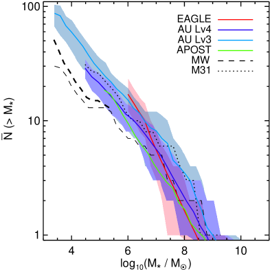
Figure 1: The satellite stellar mass function of the MW-mass haloes studied here. It shows the average number of luminous satellites per host within $300~{}\rm kpc$ as a function of satellite stellar mass, $M_{\star}$. The solid lines show median estimates and the shaded regions show 16th to 84th percentiles for the eagle (red), auriga level-4 (purple), and auriga level-3 (blue) simulations. We also indicate the median satellite stellar mass function of apostle (solid green Sawala et al., 2016). The black dotted and dashed lines give the observed satellite stellar mass function within $300~{}\rm kpc$ of the MW and M31, respectively. The thicker dashed line illustrates the incompleteness-corrected MW satellite stellar mass function (Newton et al., 2017).

To identify systems similar to the MW and M31, we start by selecting in the eagle simulation haloes with mass, $M_{200}\in[0.3,3]\times 10^{12}{~{}\rm M_{\odot}}$. The wide mass range is motivated by the large uncertainties in the total mass of the MW (e.g. Fardal et al., 2013; Cautun et al., 2014b; Piffl et al., 2014; Wang et al., 2015; Han et al., 2016) and the need to have a large sample of such systems. We further select isolated haloes by excluding any central galaxy that has a neighbour within $600~{}\rm kpc$ with a stellar mass larger than half their mass. We also restrict our selection to haloes that, like the MW, have at least 11 luminous satellites within a distance of $300~{}\rm kpc$ from their central galaxy. eagle contains 1080 host haloes that satisfy all the selection criteria; the sample has a median halo mass, $M_{200}\sim 1.2\times 10^{12}{~{}\rm M_{\odot}}$, and, on average, $15$ luminous satellites per halo. For the auriga simulation, we use all the 30 systems, which were selected in the first place to be isolated and to have halo masses similar to the MW halo mass. For both simulations, we only consider luminous satellites, defined to be subhaloes with at least one star particle. Selecting substructures with one or more star particles means that these substructures are luminous and that we capture any biases between luminous and dark subhaloes, if such biases are present. Apart from random effects arising from the stochastic nature of star formation in the simulations, this sample selection is robust. A higher resolution simulation with identical subgrid physics would, on average, assign the same luminosity to the same haloes in the current simulation although with more (less massive) star particles.

Fig. 1 investigates the satellite stellar mass function of the two simulations within a distance of $300~{}\rm kpc$ from each central galaxy. We find good agreement between eagle and auriga medium resolution, with the only noticeable discrepancy being for $M_{\star}<10^{7}{~{}\rm M_{\odot}}$, which is close to the resolution limit of eagle. The stellar mass function of the auriga high-resolution sample is systematically higher than both eagle and auriga level-4 ones; this likely is due to the small number (6) of high-resolution system and due to the fact that these systems have halo masses, on average, 10% more massive than those in the full auriga sample. The eagle and auriga results are consistent with the apostle ones (Sawala et al., 2016), which is another suite of zoom-in simulations of paired MW-mass haloes chosen to resemble the Local Group (Fattahi et al., 2016).

Fig. 1 also shows that the dwarf stellar mass functions found in our simulations are consistent with the ones observed around the MW and M31 (see also Sawala et al., 2016; Simpson et al., 2017), which we take from the McConnachie (2012) compilation. The agreement is especially good with the M31 observations, whereas the MW data is systematically lower, especially for satellites less massive than $10^{7}{~{}\rm M_{\odot}}$. The MW satellite stellar mass function is affected by incomplete sky coverage; accounting for this using the Newton et al. (2017) predictions pushes up the faint end of the MW dwarf count, but not enough to fully account for the difference. The discrepancy could be due to combination of factors, such as the total MW halo mass being lower than that of our sample, the MW having an atypically low number of satellites for its mass, or a higher than accounted for observational incompleteness of MW surveys as argued by Yniguez et al. (2014).

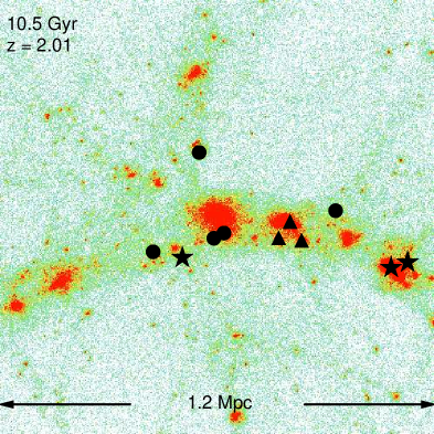
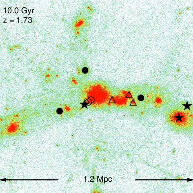
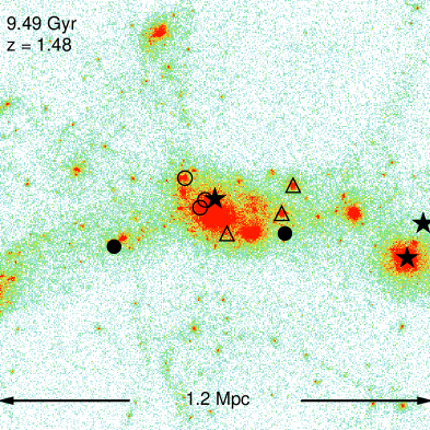
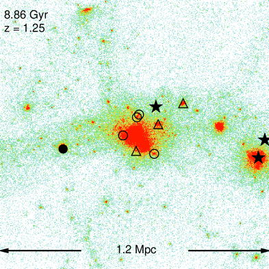
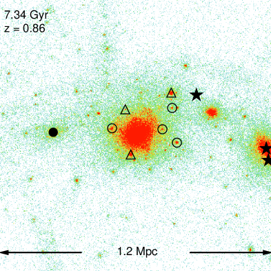
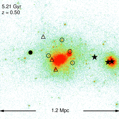
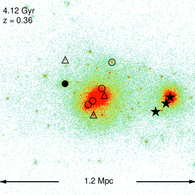
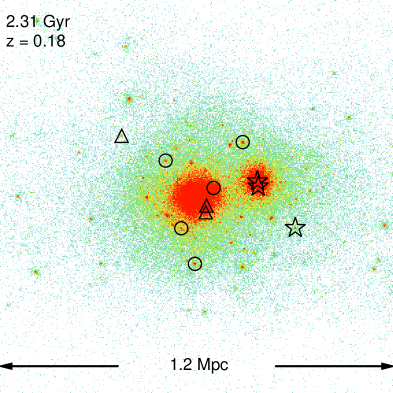
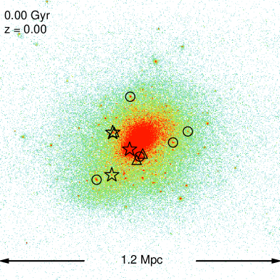
Figure 2: Evolution of a eagle MW-mass system since $z=2.01$ to present day. The colours indicate the DM distribution within a $1.2~{}\rm{Mpc}$ physical box centred on the halo position, with red showing high-density regions. The black symbols indicate the positions of the progenitors for the 11 $z=0$ satellites with the largest stellar mass. These 11 satellites were accreted in two groups of multiplicity, $\rm m_{11}=3$, with the members of those groups shown as star and triangle symbols, while the remaining satellites were accreted singly and are shown as circles. The satellite progenitors are shown as filled symbols before infall, and as open symbols after infall into the host halo.

3 Results

Here we study the fraction of satellites that were accreted as groups or along the same filament, after which, we quantify the anisotropies in the accretion of satellites by investigating the alignment of the infall direction of each satellite with the preferential axes of its host systems. We end with an analysis of the connection between group and filamentary accretion with the MW disc of satellite galaxies, i.e. the structures present in the spatial and kinematic distribution of the Galactic satellites.

3.1 Multiplicity of satellite accretion

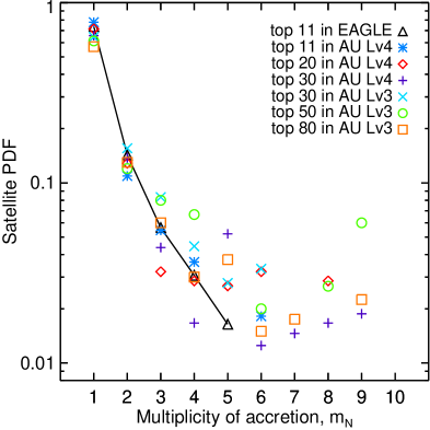
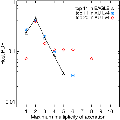
Figure 3: The PDF of the multiplicity of accretion for the top $N$ satellites with the largest $z=0$ stellar mass. Top panel: the vertical axis gives the fraction of satellites accreted in groups of that given multiplicity, with $m_{N}=1$ corresponding to singly accreted satellites. The various symbols correspond to different values of $N$ and to different simulations, which are eagle, and auriga medium (level-4) and high resolution (level-3), as indicated in the legend. For readability, the eagle results are shown as triangles connected with a solid line. Bottom panel: the vertical axis gives the fraction of hosts as a function of their maximum multiplicity of accretion, i.e. the number of objects in the richest accreted satellite group. We show results only for eagle (1080 hosts) and auriga level-4 (30 hosts) using the same symbols as in the top panel.

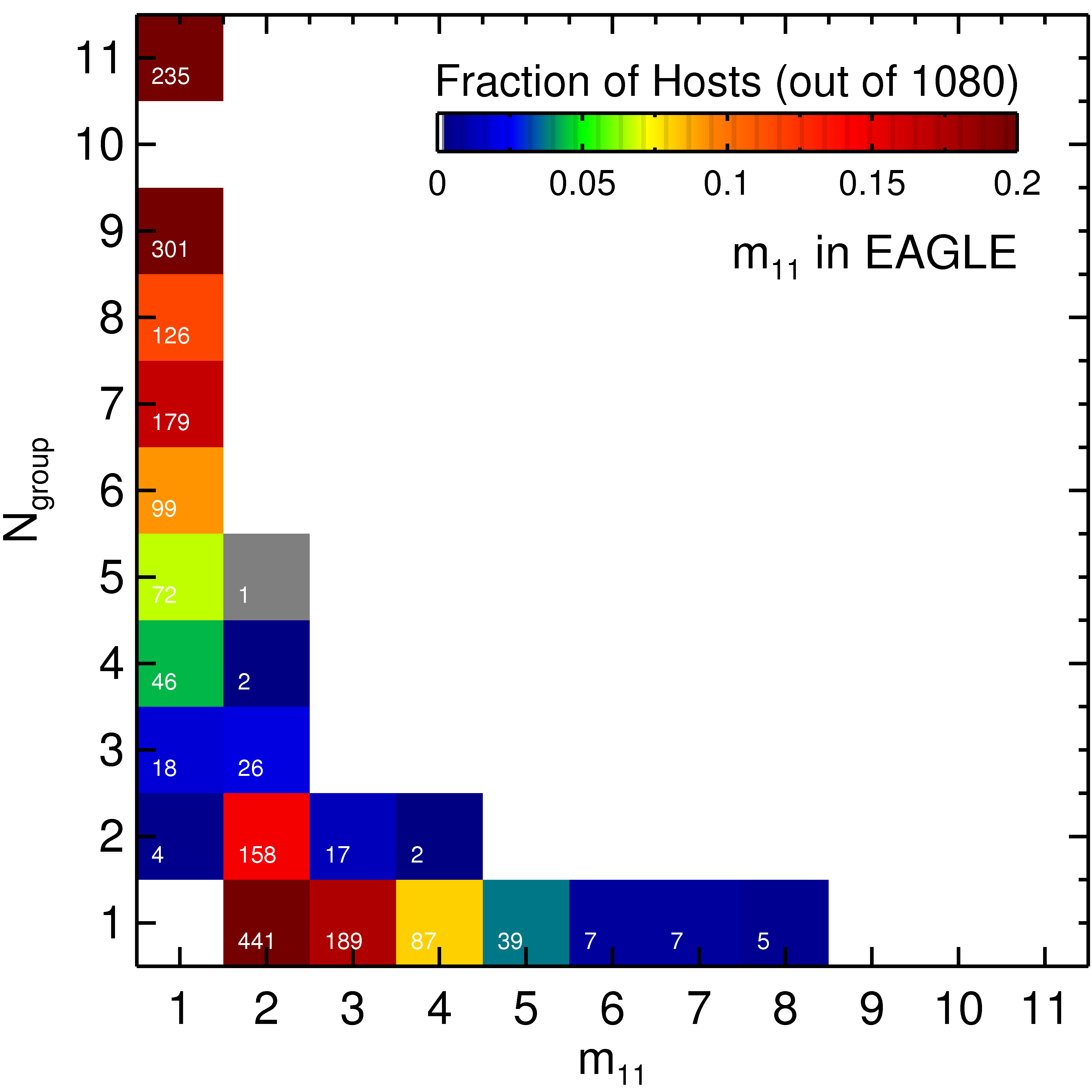
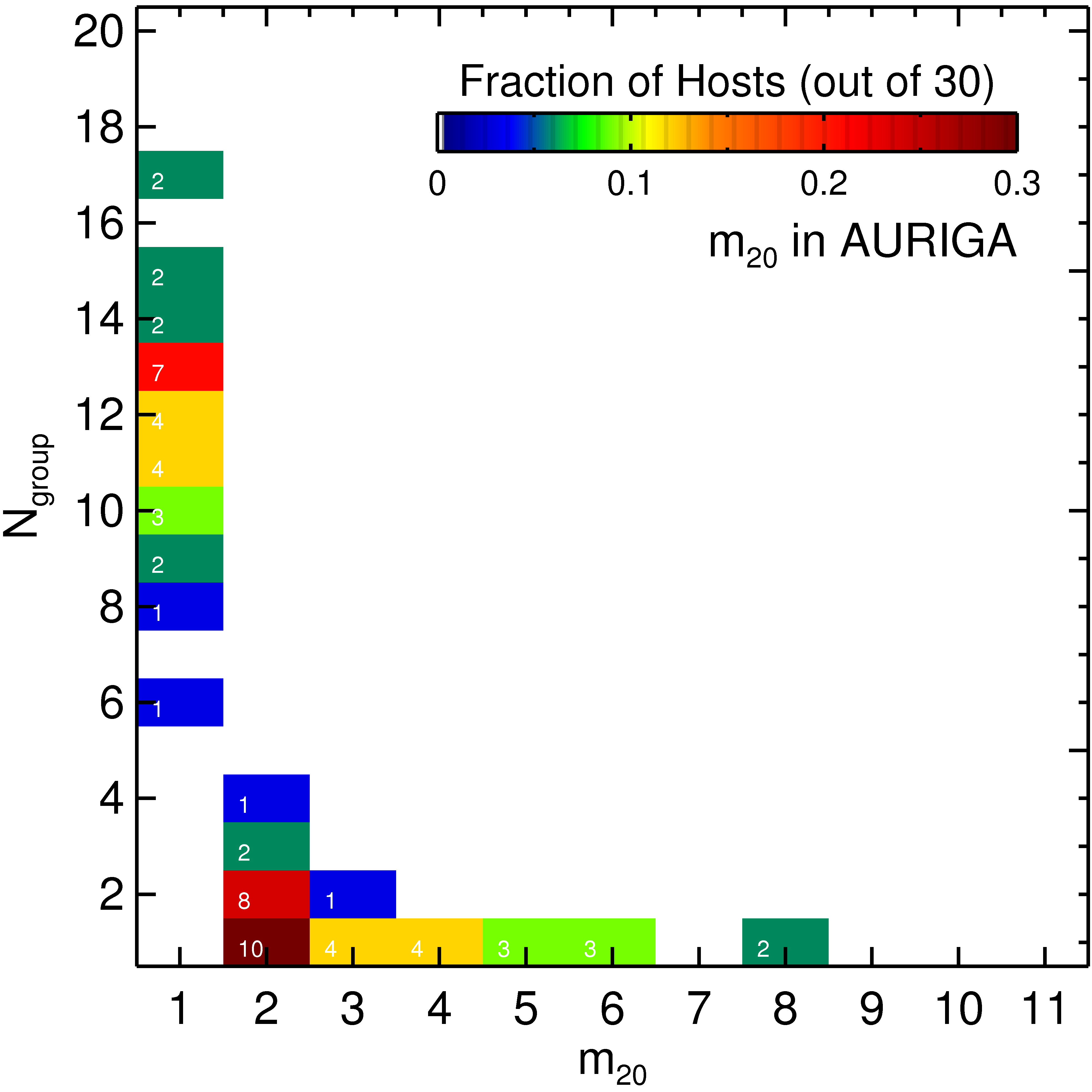
Figure 4: Histogram of the multiplicity of satellite accretion in the eagle (top panel) and the auriga level-4 (bottom panel) MW-mass halo samples. The top and bottom panels show the multiplicity of accretion, $m_{11}$ and $m_{20}$, for the respectively 11 and 20 satellites with the largest present-day stellar mass. The colours indicate the fraction of haloes with a given satellite accretion history, e.g. in the top panel the $(m_{11}=1,~{}N_{\rm{group}}=6)$ point shows that 9% of haloes had accreted six groups with multiplicity 1, and the $(m_{11}=2,~{}N_{\rm{group}}=2)$ point shows that 15% of haloes accreted two groups of multiplicity 2. The number inside each histogram entry gives the count of host haloes (out of 1080 for the top panel and out of 30 for the bottom one) with that satellite accretion history.

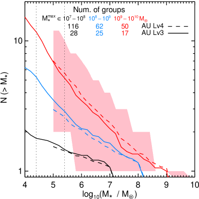
Figure 5: Stellar mass function of satellites of satellites that were accreted into MW-mass haloes. The curves are split according to the stellar mass of the primary object, which is the galaxy in the group with the largest stellar mass before accretion into the MW-sized host halo. We show three bins in primary stellar mass, $10^{9}-10^{10}$ (red), $10^{8}-10^{9}$ (blue), and $10^{7}-10^{8}$ ${~{}\rm M_{\odot}}$ (black), for both auriga level-4 and level-3 simulations, and we give in the legend the number of groups contained in each subsample. The dashed and solid lines show the average satellites-of-satellites count for the medium and the high-resolution simulations. The shaded region shows the 16th to 84th percentile range, which, for clarity, we only show for the most massive subsample in auriga level-4. The vertical dotted lines indicate five times the initial gas element mass for the two resolution levels.

Our goal is to study the accretion of the present-day brightest $N$ satellites, which we select as the $N$ satellites with the largest $z=0$ stellar mass and that are within a distance of $300~{}\rm kpc$ from the central galaxy. We refer to these objects as the top $N$ satellites and we vary $N$ from 11, corresponding to the MW classical satellites, to 80, which is determined by the smallest number of satellites across each of the six auriga high-resolution haloes. For each of the top $N$ satellites, we calculate the multiplicity of accretion, $m_{N}$, as the number of top $N$ satellites that were part of the same group at accretion into the host halo.

For each central and satellite galaxy, we trace their formation history using the eagle and auriga merger trees for the most massive progenitor. Starting at high redshift, we follow forward the merger trees of each satellite in tandem with the merger tree of its central galaxy, until we find the first snapshot where the satellite and the central are part of the same FOF group; this corresponds to the snapshot when the satellite was first accreted on to its $z=0$ host halo. Then, the group ID in which that satellite was accreted is given by the FOF halo ID of its progenitor at the snapshot just before first accretion. We repeat this procedure for the top $N$ satellites of each host, and, once finished, count how many satellites have the same group ID just before accretion. Groups are defined as the subset of galaxies that in the snapshot just before accretion were part of the same FOF group. We do not require that they be gravitationally bound, so a small fraction of groups could potentially contain unbound members that fell into the host halo at the same time and along a similar direction.

Fig. 2 illustrates the evolution of the progenitors for the top 11 present-day satellites of one eagle halo. This system has two group accretion events each with three satellites that are part of the top 11 $z=0$ satellites. The satellites accreted in the two groups are shown as triangle and star symbols, while the remaining satellites, which were accreted singly, are shown as circles. The triplet shown with triangles is accreted early, being already part of the same FOF halo in the second panel of Fig. 2. This group was probably loosely bound, because, in the subsequent frames, its three members are spread over most of the halo; however, in the last two frames, two of these members form a tightly bound pair. The second triplet, which is shown as stars, has a different evolution history. Two of its members were a long-lived group since at least the top-left panel, while the third member falls in along a different filament and only becomes part of the triplet shortly before accretion, which takes places at $z\simeq 0.2$.

The top panel of Fig. 3 quantifies the probability distribution function (PDF) that a satellite was accreted singly, i.e. $m_{N}=1$, or as part of a group, i.e. $m_{N}\geqslant 2$, for different populations of top $N$ satellites, with $N$ ranging from 11 (corresponding to the classical MW satellites) to 80. The top 11 satellites are predominantly accreted by themselves, which happens in 75% of cases. Group accretion is dominated by pairs, 14% of the time, and triplets, 6% of the time, whereas rich groups with $m_{N}\geq 6$ represent 1% of cases. As we increase $N$ and we study a larger number of top satellites, we find that a larger fraction of satellites are accreted in groups. For example, using the high-resolution auriga simulations we find that the top 50 satellites were accreted singly 60% of the time, in pairs 12% of the time, and in groups of six or more members 12% of the time. The results for top 50 satellites, while limited by the small number of systems (6 hosts with 300 satellites), confirm the trend of group accretion to become more important for the faint satellites and agree with the trends found by previous studies, based on dissipationless simulations coupled with semi-analytic galaxy formation models or abundance matching (Wang et al., 2013; Wetzel et al., 2015).

The multiplicity of group accretion can be quantified from the perspective of the host halo. The bottom panel of Fig. 3 shows the fraction of MW-sized hosts that have a given maximum multiplicity of accretion. When considering the top 11 satellites in eagle, the most likely outcome is the accretion of one or more satellite pairs (45% of cases), followed by hosts that accreted all their satellites singly (23% of cases). The accretion probability of triplets and richer groups decreases rapidly, with 18, 8, 4, 2% of MW-sized haloes accreting groups with a maximum multiplicity of 3, 4, 5, and 6 or higher, respectively. As expected, when considering fainter satellites, such as the top 20, we find that the multiplicity of the richest group increases.

Fig. 4 presents a detailed histogram of the number of groups of different multiplicities that were accreted by each host halo. Focusing first on the top 11 satellites in the eagle simulation (top panel), we find that 235 hosts (22%) accreted all their satellites singly, while less than 13% (sum of the boxes with $m_{11}=1$ and $N_{\rm group}\leq 5$) of hosts have five or fewer satellites accreted singly. For pair accretion, i.e. $m_{11}=2$, we find one extraordinary host that has accreted as many as five pairs, 26 hosts have accreted three pairs, while $\gtrsim 15\%$ of the hosts have accreted two pairs of satellites. Furthermore, by summing the numbers in the $m_{11}=2$ column, we find that $\approx 60\%$ of hosts have accreted at least one pair of satellites. For multiplicity greater than 2, we find that almost 20% and 14% of hosts have accreted one group with multiplicity, $m_{11}=3$ and $m_{11}\geq 4$, respectively. The plot suggests that the probability of most of the top 11 satellites to be accreted as a single group is very small, with less than 2% of our MW-mass sample having accreted a group with multiplicity of 6 or higher.

The bottom panel of Fig. 4 shows the multiplicity of accretion histogram for the top 20 satellites in the auriga level-4 simulations. Of the 30 auriga systems, two are dominated by singly accreted satellites, that is the ones with $m_{20}=1$ and $N_{\rm group}=17$, and none of the auriga hosts has only singly accreted satellites. For multiplicity $\rm m_{20}=2$, we find that $\approx 70\%$ of the haloes (21 out of 30) have accreted at least one pair of satellites, which is 10% higher than the fraction for the top 11 satellites. For higher multiplicities, the small number of auriga hosts limits the extent to which we can make statistically robust assertions.

We have shown that a sizeable fraction of the top $N$ satellites were accreted in groups. The richness of such groups is likely correlated to the total halo mass of the group, with more massive groups bringing in a larger number of satellite galaxies. This raises the question: how many satellites would an LMC or an SMC mass galaxy bring with it? We investigate this in Fig. 5, where we plot the satellite stellar mass function of groups at infall. The satellites of these groups, once accreted, become satellites of satellites. We further split the groups into subsamples according to the stellar mass of the most massive member of the group, which can also be done in observations. Groups in which the dominant galaxy has a stellar mass of $10^{9}-10^{10}{~{}\rm M_{\odot}}$, which includes the LMC, bring in a considerable contingent of satellites, and have $3$, $7$ and $15$ members with stellar masses higher than respectively $10^{6}$, $10^{5}$ and $10^{4}{~{}\rm M_{\odot}}$, which is in agreement with the abundance matching predictions of Dooley et al. (2017). We checked that restricting the selection criteria to groups where the dominant galaxy has a stellar mass in the range $1-4\times 10^{9}{~{}\rm M_{\odot}}$, which corresponds to the LMC stellar mass, we get the same satellites-of-satellites mass function. Compared to the MW, which for the same stellar masses has about 7, 13 and 20 satellites, the LMC could have brought a modest, but non-negligible, number of its own satellites. The scatter in the satellite stellar mass function of LMC-mass groups is considerable, which is probably a manifestation of the large scatter between stellar mass and halo mass for LMC-sized dwarf galaxies (Schaye et al., 2015; Sawala et al., 2015), with the satellite luminosity function expected to correlate more strongly with the total halo mass. Groups that host less massive dominant galaxies bring in fewer satellites, with SMC-sized (stellar mass range of $10^{8}\sim 10^{9}{~{}\rm M_{\odot}}$) and Fornax-sized (stellar mass range of $10^{7}\sim 10^{8}{~{}\rm M_{\odot}}$) groups bringing respectively six and two members more massive than $10^{4}{~{}\rm M_{\odot}}$.

3.2 Filamentary accretion

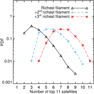
Figure 6: The PDF of the number of top 11 satellites accreted along the richest (solid black), the two richest (dashed blue) and three richest (dotted red) filaments in the eagle simulation. The filament richness is given by the number of satellites accreted along that filament.

Filamentary accretion of satellites is an ubiquitous feature of structure formation within $\Lambda$CDM, and, similarly to group accretion, enhances the spatial and orbital anisotropies of the satellite distribution. The filaments act as channels that transport dwarf galaxies and that funnel their infall into MW-sized haloes (e.g. Libeskind et al., 2005, 2014; Buck et al., 2015; González & Padilla, 2016). Here, we consider that two satellite galaxies were accreted along the same filament if they entered their host halo along approximatively the same direction. This definition is motivated by two observations. First, the prominent massive filaments remain quite stable in time, with most of the evolution of the filamentary network involving only the thin tenuous filaments (Rieder et al., 2013; Cautun et al., 2014a). The massive filaments are the main mass accretion pathways into the halo and thus they are the ones along which most satellites fall in (Danovich et al., 2012). Secondly, filamentary accretion is more likely to lead to co-planar orbits if two satellites enter their host halo at roughly the same points.

The more massive a satellite is, the more likely it is that it was accreted along the spine of a filament (Libeskind et al., 2014). This suggests a simple algorithm for identifying how many of the present-day satellites were accreted along the same filament, i.e. along the same direction. Starting with the most massive satellite, we compute the angle between its entry direction and that of the remaining top $N$ satellites. Then, all the satellites within an opening angle of $30^{\circ}$ are assigned to the first filament. We then go to the next most massive satellite that is yet to be assigned to a filament and compute the angle between its entry direction and that of the other satellites not assigned to filaments. The second filament contains all the satellites within the same opening angle of $30^{\circ}$. We iteratively apply this procedure until all satellites are assigned to one filament. Similarly to group accretion, filamentary accretion is defined using the satellite entry points in the host FOF halo. We checked that we obtain mostly the same filaments if instead we use the satellite entry points measured on a uniform sphere outside the host halo. We refer to the number of satellites associated with each filament as the filament richness, and we order the filaments in decreasing order of their richness. The richest filaments are likely to correspond to the prominent filaments feeding MW-mass haloes, with each MW-mass halo having at least two or three such objects (Danovich et al., 2012; Cautun et al., 2013, 2014a; González & Padilla, 2016).

The choice of $30^{\circ}$ opening angle corresponds to the typical angular size of dwarf groups at infall as seen from the centre of the MW-mass host halo. This ensures that if the primary dwarf galaxy of that group is assigned to a certain filament, then all the other group members are also assigned to that filament. The $30^{\circ}$ opening angle corresponds to a solid angle of $0.27\pi$ and represents $\sim 1/15$ of the full sky. Thus, this opening angle is small enough, such that, if the top 11 satellites were accreted isotropically, no two satellites would have to be part of the same filament.

Fig. 6 shows the satellite galaxies count brought in by the top $i\rm{th}$ ($i=1,2,3$) richest filaments in the eagle simulation. The distribution of the richest filament shows that for all hosts the richest filament contains two or more galaxies that fell along it. Thus, in none of the hosts, were the satellites accreted from 11 directions separated by more than $30^{\circ}$ each. The richest filament is most likely to contain three satellites (40% of cases), followed by four satellites in 25% of the cases. In 20% of the hosts five or more satellites are accreted along the richest filament. The curve for the top two richest filaments peaks at a value of 5$-$6 suggesting that typically half of the top 11 satellites were accreted along just two filaments, with 80% of hosts having accreted at least five satellites along those two filaments. Furthermore, 70% of the hosts have at least seven satellites in their top three richest filaments. If satellite accretion directions were distributed isotropically, only 45% of hosts would have similarly rich top three filaments (see Appendix A for details), which illustrates the anisotropic and filamentary nature of dwarf galaxy accretion.

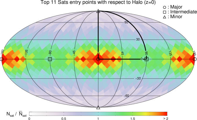
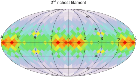
Figure 7: Aitoff sky projections of the entry points of the top 11 satellites in the eagle simulation. To stack all the hosts, we expressed the entry point in a coordinate system given by the preferential axes of the $z=0$ DM halo shape, with the main, intermediary, and minor axes corresponding to the points $(0,0)$, $(90,0)$ and $(0,90)$ degrees, respectively (see the legend of the top panel). The colour scale is the same for all panels and shows the number of satellites in HEALPix pixels normalized by the mean expectation for isotropic accretion. The halo shape determines an orientation, not a direction, which means that all the relevant information is contained in one octant of the sphere (the thick solid line in the top panel shows one such octant); this explains the symmetries of the projection. The top panel shows the entry points of all satellites, the middle one shows the entry points of group (left) and single (right) accretion events, and the bottom one shows the positions of the richest (left) and second richest (right) filaments.

3.3 Anisotropy of accretion

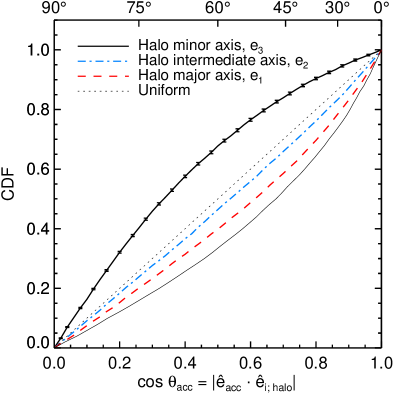
Figure 8: The cumulative distribution function (CDF) of the accretion misalignment angle, $\theta_{\rm acc}$, between the entry points of the top 11 satellites and the major (dashed line), intermediate (dash-dotted line) and minor axes (thick solid line) of the shape of their $z=0$ host haloes in the eagle simulation. The error bars around the thick solid line indicate the $1\sigma$ uncertainty range, which has the same size for all the curves. The thin dotted line corresponds to a uniform distribution. The thin solid line is the mirror image of the thick solid line with respect to the uniform line; it shows that the largest alignment is with the halo minor axis. The error bars shown here and in the subsequent figures show the 68 percentile bootstrap uncertainties calculated using 200 samples.

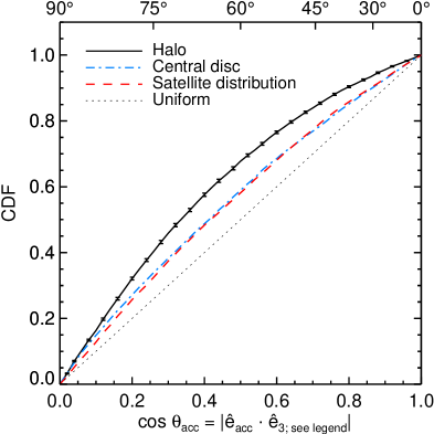
Figure 9: The CDF of the accretion misalignment angle, $\theta_{\rm acc}$, between the entry points of the top 11 satellites and the shape minor axis, $e_{3}$, of their $z=0$ host haloes (solid line), central galaxies (dash-dotted line), and top 11 satellite distributions (dashed line) in the eagle simulation.

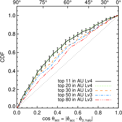
Figure 10: The CDF of the accretion misalignment angle, $\theta_{\rm acc}$, between the entry points of the top $N$ satellites and the shape minor axis of their $z=0$ host haloes. The various curves show the dependence of the CDF on $N$ in the auriga medium- (level-4) and high-resolution (level-3) simulations. The eagle top 11 results agree well with the auriga level-4 top 11 ones and, for readability, are not shown in the figure.

To study the anisotropy of satellite accretion in the eagle simulations, we examine the entry points of the top 11 satellites. As described in Sec. 2.1, starting at high redshift, we trace the top 11 satellites forward up to the first simulation output when they become part of the same FOF group as the progenitor of their present day MW-mass host; this determines the accretion time. Then, using the snapshot just before accretion, we define the entry point of each satellite as the position of the satellite progenitor with respect to the central galaxy progenitor.

We calculate the accretion anisotropy with respect to the $z=0$ shapes of the DM host halo, central galaxy and the top 11 satellite distribution. The shape is determined from the mass tensor,

$$I_{ij}\equiv\sum_{k=1}^{N}m_{k}x_{k,i}x_{k,j}\;,$$ (1)

where $N$ is the number of tracers, which are DM particles for the halo, stars for the central disc and the top 11 satellites for the satellite distribution. For the halo we limit our calculation to all particles included within $\rm R_{200}$, while for the central galaxy we use all the stars within $10~{}\rm kpc$ from the galaxy centre. The quantity $x_{k,i}$ denotes the $i$th component ($i=1,2,3$) of the position vector of tracer $k$ with respect to the halo centre, and $m_{k}$ denotes that tracer’s mass. For the shape of the satellite population, we weigh equally all satellites by assigning them the same mass. The shape and the orientation are determined by the eigenvalues, $\lambda_{i}$ ($\lambda_{1}\geqslant\lambda_{2}\geqslant\lambda_{3}$), and the eigenvectors, $\boldsymbol{\mathit{\hat{e}}}_{i}$, of the mass tensor. The major, intermediate and minor axes of the corresponding ellipsoid are given by $a=\sqrt{\lambda_{1}}$, $b=\sqrt{\lambda_{2}}$, and $c=\sqrt{\lambda_{3}}$, respectively.

In Fig. 7, we show the entry points of the top 11 satellites of eagle MW-sized hosts. To stack all the hosts, we expressed the entry directions into a common coordinate system, which we chose as the eigenvectors of the shape of the DM halo. As we will discuss shortly, satellite accretion shows the strongest alignment with the halo shape, which represents the motivation for our choice of coordinate system. The eigenvectors determine only an orientation and do not have a direction assigned to them, so, when expressed in the halo shape eigenframe, we mirror each entry point eight times: two times for each Cartesian coordinate. This means that independent information is contained in only one octant of the sky plot; however, for clarity, we choose to present the full sky distribution. By stacking the top 11 satellites of all the $1080$ MW-sized hosts, we have a sample of $11880$ entry points which allows for a statistically robust characterization of dwarf galaxy accretion anisotropies. The 3D entry direction of each satellite is expressed in spherical angular coordinates and pixlized using the HEALPix public code.

The top row in Fig. 7 shows that satellite accretion is highly anisotropic, with dwarf galaxies being preferentially accreted within $20^{\circ}$ from the equatorial plane, which is determined by the major and intermediate axes of the DM halo, and, within this plane, satellite accretion shows a pronounced excess along the halo major axis. This not only confirms the anisotropic accretion results found by previous studies (Libeskind et al., 2011; Libeskind et al., 2014; Kang & Wang, 2015; Wang & Kang, 2018), but extends those results to hydrodynamic simulations (see Garaldi et al., 2018) and to a large sample of MW-sized haloes, which allows us to robustly quantify anisotropic accretion. The marked alignment between halo shape and satellite infall is due to both mass and satellites being preferentially accreted along a few massive filaments; this filamentary infall is the one giving rise to the alignment of both DM halo shape (Zhang et al., 2009) and satellite galaxies (Tempel et al., 2015) with the cosmic web filaments.

The middle row in Fig. 7 illustrates how the anisotropy of accretion for the top 11 satellites varies between group and singly accreted dwarfs. Compared to single accretion events, galaxies that arrive with one or more companions (20% of the population) are more strongly clustered along the equatorial plane of the projection and especially along the halo major axis. This is to be expected, since on average groups of dwarfs reside in more massive subhaloes than single dwarfs at accretion, and more massive subhaloes are more likely to be accreted along filaments than less massive ones (Libeskind et al., 2014). This strong correlation between group and filamentary accretion is emphasized by the bottom row of Fig. 7, which shows the entry points of the dwarfs that were accreted along the richest and second richest filaments. The satellites that fell in along the richest filament (42% of the population) are strongly clustered along the halo major axis, very similar to the clustering of group accretions. The second richest filament is preferentially located within the equatorial plane and roughly randomly oriented within this plane.

To better quantify the anisotropy of satellite accretion, we define the accretion misalignment angle, $\theta_{\rm acc}$, between the satellite entry point and the present-day DM halo, central disc or satellite distribution. The misalignment angle is given by

$$\cos\theta_{\rm acc}=|\boldsymbol{\mathit{\hat{e}}}_{\rm acc}\cdot\boldsymbol{\mathit{\hat{e}}}_{i;~{}\rm{X}}|\;,$$ (2)

where $\boldsymbol{\mathit{\hat{e}}}_{\rm acc}$ is the unit vector pointing along the satellite entry point, and $\boldsymbol{\mathit{\hat{e}}}_{i;~{}\rm{X}}$ ($i=1,2,3$) are the principal axes of the $z=0$ shape of the: DM halo ($\rm{X=halo}$), central disc ($\rm{X=disc}$) or satellite distribution ($\rm{X=sats}$).

We start by studying the misalignment angle between satellite accretion and present-day DM halo shape, which is shown in Fig. 8. Satellite accretion tends to be well aligned with the major axis (median angle $52^{\circ}$), to be less aligned with the intermediate axis (median angle $57^{\circ}$), and to be preferentially perpendicular to the minor axis (median angle $70^{\circ}$). To compare the three signals, we mirror the minor axis alignment with respect to the expectation for an isotropic distribution, which is the diagonal line. We find that the accretion direction of satellites shows the largest alignment (actually a misalignment) with the halo minor axis, which suggests that the most important trend is for satellites to fall in perpendicular to the halo minor axis. We studied the misalignment angle between accretion direction and the $z=0$ central disc and satellite distribution, and, in both cases, the strongest alignment is with the minor axis, which is why in the following figures we choose to show only the alignment angle with respect to the minor axis.

Fig. 9 compares the alignment of the satellite infall directions with the $z=0$ shape minor axis of the halo, central galaxy and the top 11 satellites. Of the three, the halo minor axis shows the largest alignment (median angle $71^{\circ}$), while the central galaxies and the satellite systems show lesser degree of alignment (both have median angles of $66^{\circ}$). While central galaxies are well aligned to the innermost ${\sim}20~{}\rm kpc$ of their DM haloes (Shao et al., 2016; Gómez et al., 2017a), the galaxies show on average a $33^{\circ}$ misalignment angle with the full DM distribution within $R_{200}$ (Shao et al., 2016). The misalignment could be due to time variations in position of the filaments along which most matter is accreted into the halo (Vera-Ciro et al., 2011; Rieder et al., 2013) and due to massive substructures that can torque the inner disc (Gómez et al., 2017a; Gómez et al., 2017b). Similarly, the satellite distribution also shows a $33^{\circ}$ misalignment angle with the full DM halo (Shao et al., 2016), which could be due to the satellites representing a stochastic sampling of the DM distribution (Hoffmann et al., 2014). Shao et al. (2016) pointed out that the present-day central galaxy – satellite system alignment is a consequence of the tendency of both components to align with the DM halo. This could also be the case for the alignment of the infall directions. For example, the alignment of the central galaxy with the halo, which in turn is aligned with the satellite infall direction, would result in a weak alignment between the central galaxy and the satellite infall direction, which is what we measure.

In Fig. 10 we study how the anisotropy of accretion varies as a function of satellite brightness using the auriga medium- and high-resolution simulations. The degree of anisotropic accretion decreases from bright to faint satellites, for example the median misalignment angle of the top 11 satellites is $73^{\circ}$ while for the top 80 satellites is $66^{\circ}$. This agrees and extends the results of Libeskind et al. (2014), who have shown that the most massive dark matter subhaloes are the ones that were accreted most anisotropically.

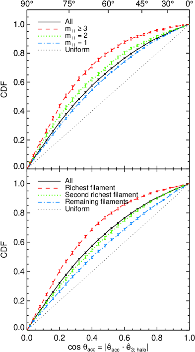
Figure 11: The CDF of the accretion misalignment angle, $\theta_{\rm acc}$, between the entry points of the top 11 satellites and the shape minor axis of their $z=0$ host haloes in the eagle simulation. The black line shows the full sample alignment while coloured lines correspond to subsamples. In the upper panel, satellites are split according their multiplicity of accretion, $\rm m_{11}$, while in the bottom panel satellites are split according to the richness of the filament they fell along. The error bars indicate the $1\sigma$ uncertainty for the various subsamples.

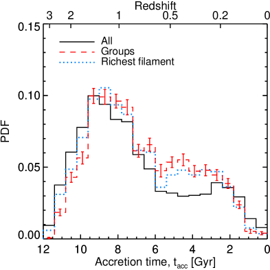
Figure 12: The distribution of top 11 satellites’ accretion lookback time, $t_{\rm acc}$, in eagle for the full sample (solid line), and for two subsamples: satellites that were accreted in groups, i.e. $\rm m_{11}\geq 2$ (dashed line), and those that were accreted along the richest filament (dotted line). The error bars indicate the $1\sigma$ uncertainty range, which, for clarity, we show only for the subsample with the smallest size: satellites accreted in groups.

In Fig. 7, we found that satellites accreted in groups and those along the richest filaments show a larger degree of anisotropic infall than the whole population. We further quantify this effect in Fig. 11, where we present the misalignment angle between infall direction and the DM halo minor axis for a subsample of satellites selected according to their group multiplicity (top panel) or filament richness (bottom panel). Rich groups, that is with a multiplicity of at least 3, show a much larger misalignment than the full satellite population. A similar trend is observed for pair accretion too, though in this case the difference with the full sample is smaller. Singly accreted satellites show roughly the same alignment, albeit slightly weaker, than the full sample. The entry points of satellites that fell in along the richest filament are more anisotropic than the whole population, while dwarfs associated with the second richest and lower richness filaments have a similar anisotropy, which is weaker than that of the full sample.

Satellites that fell in as part of a group or along the richest filament have on average a later accretion time than the full sample. This is illustrated in Fig. 12, which shows the distribution of accretion times, with $t=0$ corresponding to present day. The accretion time distribution is wide, with the full sample of top 11 satellites having a typical accretion time, $t=8.5$ Gyr. Compared to the whole sample, satellites accreted in groups and along the richest filament have systematically late accretion time, with few objects accreted before $t=11$ Gyr and a considerable excess of objects with $t\leq 6$ Gyr. Multiply accreted satellites are more likely to have fallen in inside massive haloes, which, since those haloes needed time to grow, could explain why they were accreted later. Galaxies falling in along filaments are more likely to be on radial orbits and thus more likely to be disrupted (González & Padilla, 2016), and thus the surviving satellites are more likely to be recently accreted ones that were not inside their $z=0$ MW hosts for enough time to experience significant tidal stripping. While not shown, we also find a slight tendency for late accreted satellites to have infall directions that are more aligned with the present-day halo than early accreted objects. But this trend is not strong enough to explain the results of Fig. 11, that is the larger accretion anisotropy of satellites associated with groups and to the richest filament.

3.4 Implications for the MW disc of satellites

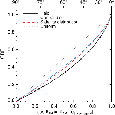
Figure 13: The CDF of the orbital pole misalignment angle, $\cos(\theta_{\rm AM})$, between the $z=0$ orbital angular momentum vector of the top 11 satellites and the shape minor axis, $e_{3}$, of their $z=0$ host haloes (solid line), central galaxies (dash-dotted line), and top 11 satellite distributions (dashed line) in the eagle simulation.

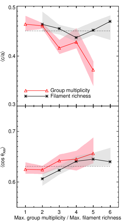
Figure 14: Upper panel: the median flattening, $c/a$, of the top 11 satellite distributions as a function of the maximum group multiplicity (red triangles) and the maximum filament richness (black squares) of the host halo. Bottom panel: the median orbital pole angle, $\cos(\theta_{\rm AM})$, between the satellite orbital angular momentum and the minor axis of the satellite distribution as a function of maximum group multiplicity and maximum filament richness. Solid lines and shaded regions indicate the median values of the distribution and the $1\sigma$ error in determining the median, respectively. The horizontal dotted line indicates the median value for the whole sample.

Group and filamentary accretion has been suggested as an explanation for the MW disc of satellite galaxies (e.g. Libeskind et al., 2005; Libeskind et al., 2011; Li & Helmi, 2008; Lovell et al., 2011) which consists of two main features: a very flattened spatial distribution and a large clustering of the orbital poles. Our large sample of eagle MW-mass haloes offers the perfect opportunity to check this conjuncture, which is the aim of this section.

Shao et al. (2016) studied the flattening of the top 11 satellite distribution for the same sample of eagle MW-mass haloes used here. The flattening, $c/a$, is defined as the ratio of the minor to major axes of the satellite distribution. The top 11 satellites in eagle have a large spread in $c/a$ values, with a median value $c/a\approx 0.45$ (see Fig. 2 in Shao et al. 2016). In contrast, the MW classical dwarfs have $c/a=0.183\pm 0.008$, which is in the tail of the eagle distribution, with only ${\sim}1\%$ of simulated systems having a flattening at least as extreme as the one observed for the MW. This is in general agreement, although slightly lower than previous studies (Wang et al., 2013; Pawlowski & McGaugh, 2014; Pawlowski et al., 2014). The difference could be due to tidal stripping of satellites by the baryonic disc of the central galaxy, which leads to less concentrated radial distributions of satellites (Ahmed et al., 2017; Sawala et al., 2017) and thus less flattened satellite distributions.

In Fig. 13, we present the alignment between the $z=0$ satellite orbital poles and the minor axis of the DM halo, central galaxy and top 11 satellite distribution. Although the orbital poles align with the central disc and the satellite system, the largest alignment is with the halo minor axis (median angle of $46^{\circ}$), which indicates that dwarf satellites preferentially orbit in a plane perpendicular to the halo minor axis. This result qualitatively agrees with previous literature, which studied the orbital pole – halo minor axis alignment using subhaloes (Lovell et al., 2011) or using semi-analytical galaxy formation models (Cautun et al., 2015a); a more quantitative comparison is difficult since the median alignment angle depends on the mass limit used to select the satellite sample, with faint satellites having more misaligned orbits (see Fig. 4 in Cautun et al. 2015a).

The majority of the classical MW satellites have orbital poles pointing along the normal to the Galactic plane of satellites (Pawlowski et al., 2012b), with the median orbital pole – satellite system misalignment angle being $\theta_{\rm AM}=36^{\circ}\pm 6^{\circ}$ (we obtained this value using the MW satellite positions and velocities given in Cautun et al., 2015b). In eagle, the same misalignment angle has a median value $\theta_{\rm AM}=51^{\circ}$; this is significantly less aligned than the MW value and illustrates the enhanced orbital pole clustering seen for the classical MW dwarfs.

The upper panel of Fig. 14 shows the correlation between the richest accreted satellite group and the median $c/a$ ratio, which we calculated by splitting the MW-mass halo sample according to the maximum group multiplicity of each host. We find that groups with a multiplicity of 3 or 4 already lead to slightly thinner planes, but the effect becomes especially important for groups with a multiplicity of 5 or higher. Nevertheless, accretion of such rich groups is rare, with only 4% of systems having accreted a group with multiplicity of 5 or higher. The same panel also shows the relation between the median $c/a$ value and the maximum filament richness of a host halo to find that the two are uncorrelated. It suggests that, if filamentary accretion is the explanation for flat satellite distributions, it is not simply due to many satellites falling in along the same filament, and, probably, the decisive factor is the overall configuration of filaments (see Appendix B), whose study we leave for future work. Alternatively, it has been suggested that rotating planes of satellite galaxies could be due to other processes, such as tidal dwarf galaxies (e.g. see Fouquet et al., 2012; Hammer et al., 2013).

The bottom panel of Fig. 14 shows the dependence of the median orbital pole – satellite system misalignment angle on both maximum group multiplicity and maximum filament richness of the MW-mass hosts. We find that within the error bars, the results are consistent with no dependence of the misalignment angle on either group multiplicity or filament richness. The lack of dependence on group multiplicity given that rich groups lead to a flatter satellite distribution is especially puzzling (see the top panel of Fig. 14). Rich groups typically fall in inside massive haloes, so those members galaxies can have significant velocities with respect to each other and that, in turn, can lead to different orbital planes inside their present-day MW-mass hosts. The satellites accreted along the same filament, while having roughly the same entry point in the host halo, can have different orbital momenta due to either the filament’s velocity dispersion or due to being accreted at different times.

4 Conclusions

We have used two hydrodynamical cosmological simulations, eagle and auriga, to study the accretion of dwarf galaxies into galactic mass haloes. The two simulations self-consistently incorporate the main physical processes that affect galaxy evolution and give rise to dwarf satellite stellar mass functions that are in agreement with both MW and M31 observations (see Fig. 1). This work studied MW-mass haloes (median mass ${\sim}1\times 10^{12}{~{}\rm M_{\odot}}$) and their satellite population within a distance of $300~{}\rm kpc$ from the central galaxy. When applied to eagle, the selection criteria resulted in 1080 MW-mass haloes that have at least 11 luminous satellites; this constitutes our sample of MW classical satellite analogues and its large size is ideal for a statistical study. The zoom-in auriga simulations, while having only 30 MW-sized haloes, are perfect for studying satellites with stellar mass as low as $5\times 10^{4}$ and $5\times 10^{3}{~{}\rm M_{\odot}}$ for respectively the medium- and high-resolution runs.

We investigated three aspects of dwarf galaxy accretion into MW-sized haloes: the accretion of galaxy groups, the infall along the cosmic web filaments, and the anisotropic nature of satellite accretion. Group multiplicity was defined as the number of companion galaxies that fell in as part of the same FOF group and that at $z=0$ are in the top $N$ largest stellar mass satellites, for varying values of $N$. Motivated by filamentary accretion leading to similar entry points into the host halo, filament richness was defined as the number of top $N$ dwarfs that fell into the MW-mass host within a $30^{\circ}$ opening angle. The anisotropic accretion of satellites was characterized in terms of the alignment between the satellite entry points and the preferential axes of the $z=0$ shape of the DM halo, central galaxy disc and the top 11 satellite distribution.

Our main conclusions are as follows.

1. For the present-day top 11 satellites, 75% of them were accreted by themselves, 14% in pairs, 6% as triplets and the rest as part of higher multiplicity groups (see Fig. 3).
   

2. Group accretion becomes more common when considering fainter satellite samples. For example, for the present-day top 50 satellites, 60% were accreted singly, 12% in pairs, and 28% in triplets or richer groups (see Fig. 3).
   

3. The multiplicity of infall groups depends on the stellar mass of the primary (i.e. most massive) group member. LMC-sized groups, where the primary galaxy has a stellar mass in the range $10^{9}-10^{10}{~{}\rm M_{\odot}}$, bring on average 3, 7 and 15 members with stellar mass larger than $10^{6}$, $10^{5}$ and $10^{4}{~{}\rm M_{\odot}}$ respectively. In contrast, Fornax-sized groups (primary stellar mass in the range $10^{7}-10^{8}{~{}\rm M_{\odot}}$) have on average only two members more massive than $10^{4}{~{}\rm M_{\odot}}$ stellar masses (see Fig. 5). The group-to-group variation in the stellar mass function of dwarf galaxy groups is large, with LMC-sized groups having anywhere between $2$ and $12$ (16 and 84 percentiles) members more massive than $10^{5}{~{}\rm M_{\odot}}$.

4. Of the $z=0$ top 11 satellites, 50% of them are accreted along the two most richest filaments and 70% along the three most richest filaments (see Fig. 6).
   

5. Dwarf galaxy accretion is highly anisotropic, takes place preferentially in the plane determined by the major and intermediate axes of the DM host halo shape, and, within this plane, is clustered along the shape major axis (see Figs 7 and 8). The satellite entry points are preferentially aligned with the central disc and the top 11 satellite system, but to a lesser extent than the alignment with the DM halo (see Fig. 9).
   

6. The degree of anisotropic accretion is largest for the most massive satellites and it decreases for fainter satellite samples (see Fig. 10).
   

7. Dwarfs accreted in groups and along the richest filament have infall directions that are more anisotropic than the full satellite sample (see Figs 7 and 11). It suggests that the filament that dominates the anisotropic accretion of matter, and thus determines the halo orientation, is also the one that brings both the most satellites falling in groups and the most satellites overall.

One of the goals of this paper was to understand what determines the spatial and kinematic structures seen in the Galactic distribution of satellites, the so-called MW disc of satellites. Motivated by previous literature (e.g. Libeskind et al., 2005; Libeskind et al., 2011; Li & Helmi, 2008; Lovell et al., 2011), we checked if indeed enhanced group or filamentary accretion leads to a larger amount of structure in the distribution of dwarf satellites (see Fig. 14). The accretion of very rich groups, which is rare, does lead to flatter spatial distributions, but it does not enhance the number of satellites with similar orbital poles. Such rich groups typically arrive in massive haloes and thus their members can have a large velocity dispersion, which can lead to different orbital planes. MW-mass systems that accreted most of their satellites along a single filament have the same average flattening and degree of planar orbits of their $z=0$ satellites as the overall sample. If indeed accretion along filaments is responsible for rotating planes of satellites, then our results suggest that the connection between the MW disc of satellites and filamentary accretion is not as simple as having the majority of satellites accreted along one filament, and that the important factors might be the spatial configuration and the characteristics of the filaments surrounding the host halo.

Appendix A Filament distribution

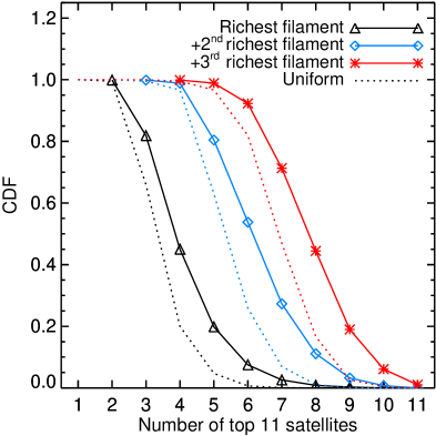
Figure 15: The CDF of the number of satellites in the richest, the two richest and three richest filaments. The solid lines with symbols show the eagle results while the dotted lines show the corresponding expectation if the satellite accretion directions are distributed isotropically on the sky.

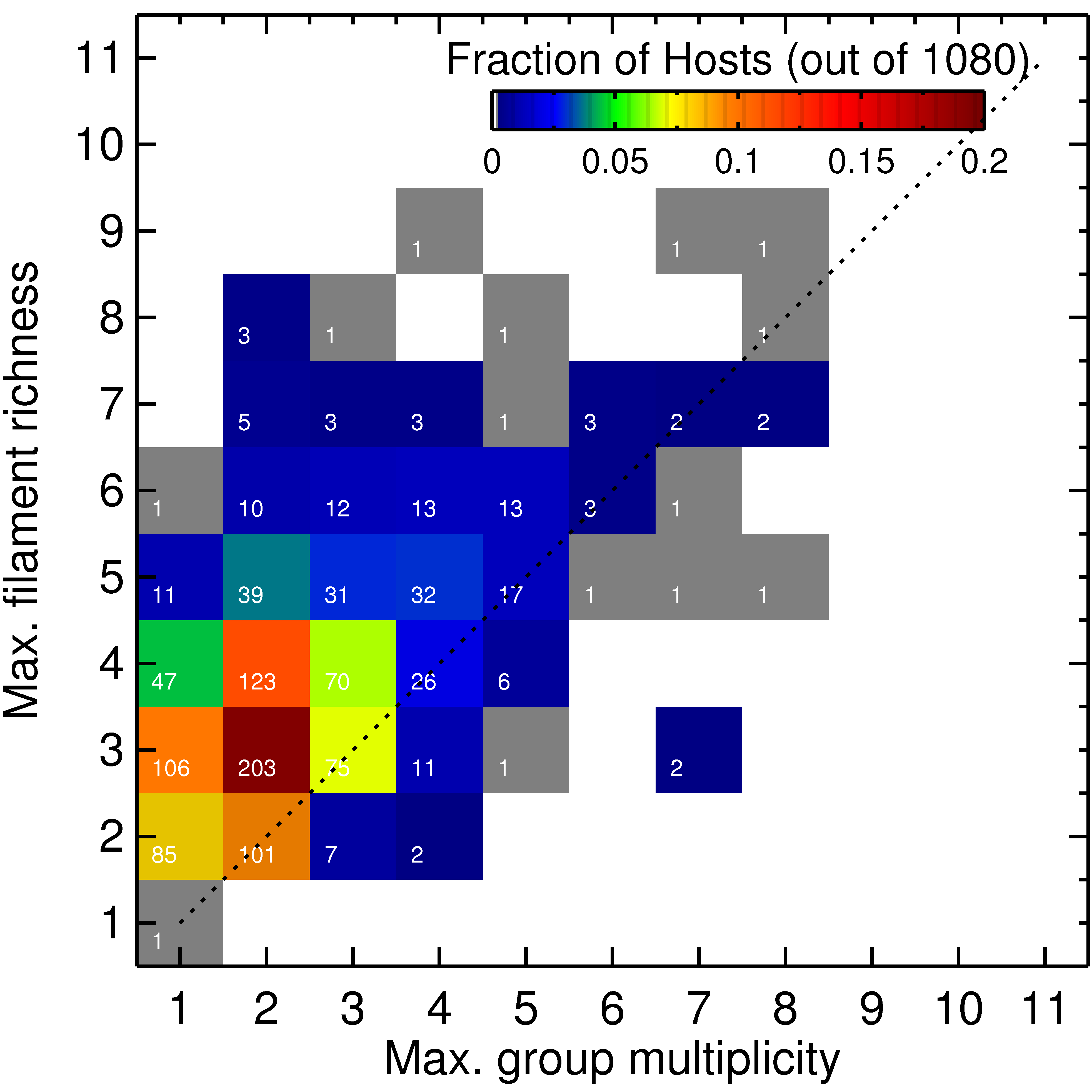
Figure 16: The maximum filament richness as a function of the maximum group multiplicity for eagle MW-mass haloes. Each square is coloured according to the fraction of the population that it contains and the numbers inside give the number of systems that contribute to that point. The diagonal line corresponds to filament richness and group multiplicity having the same value. For most cases, the richest filament has a higher richness than the richest group.

To assess the degree of filamentary accretion of satellites, it is instructive to compare to the case when the satellite entry directions are distributed isotropically on the sky. This comparison is shown in Fig. 15, where we find that $\Lambda$CDM filaments have higher richness than in the isotropic case. For example, the top filament has a richness of 4 or more in 45% of the hosts, while the isotropic accretion case results in a similarly rich top filament in only 20% of systems. Furthermore, the top three filaments bring seven or more satellites for 70% of the MW-mass haloes, while the isotropic accretion case results in similarly rich top three filaments in only 45% of systems.

In Fig. 16 we study the relation between the maximum filamentary richness and the maximum multiplicity of accretion for each of the eagle MW-mass hosts. Whereas for the majority of host haloes the top filament has higher richness than the top group, in a significant fraction of systems (21%) the top filament and the top group have the same richness. Thus, some of the richest filaments consist of satellites accreted in a single group, with no additional satellites falling in along the same direction. Furthermore, for a very small fraction of the eagle systems (3%) the top filament is less rich than the top group. This is due to the groups that have sizes on the sphere of the sky larger than a $30^{\circ}$ opening angle, which is the value used to define filaments. The large size of some groups could be due to them living in massive hosts, which could be the case for the very rich groups (e.g. group multiplicity $\gtrsim 5$), whereas the low-multiplicity groups are likely due to interloper members that are misidentified as being part of an extended FOF group.

Appendix B The connection between satellite planes and anisotropic accretion

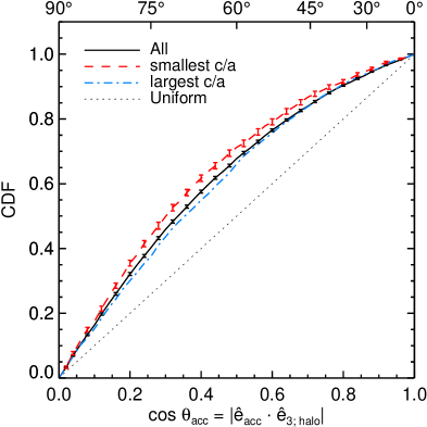
Figure 17: The CDF of the accretion misalignment angle, $\theta_{\rm acc}$, between the entry points of the top 11 satellites and the shape minor axis of the $z=0$ host halo. It shows the full sample (solid black) and two subsamples consisting of the 20% of eagle host haloes with the smallest (red dashed) and largest (blue dot-dashed) $c/a$ values for the top 11 satellite distribution.

Here we study in more detail the factors that could explain the flattening of the classical Galactic satellites. We split the eagle halo into two subsamples according to the $z=0$ flattening of the top 11 satellite system, as measured by the $c/a$ ratio (see Fig. 2 in Shao et al. 2016 for the $c/a$ distribution). We select the 20% of MW-mass haloes that have the thinnest ($c/a<0.33$) and the thickest ($c/a>0.57$) satellite distributions. Fig. 17 shows the accretion misalignment angle between the satellite entry points and the shape minor axis of the $z=0$ DM halo for the two subsamples. Present-day satellite systems that are thin are more likely to have more anisotropic accretion, while the converse is true for thicker satellite systems. Similarly, while not shown, we have also studied the alignment between satellite entry points and the minor axis of the present-day satellite system to find a similar correlation: thinner $z=0$ satellite distributions correspond to more anisotropic accretion.

References

- Ahmed et al. (2017) Ahmed S. H., Brooks A. M., Christensen C. R., 2017, MNRAS, 466, 3119
- Angulo et al. (2009) Angulo R. E., Lacey C. G., Baugh C. M., Frenk C. S., 2009, MNRAS, 399, 983
- Aubert et al. (2004) Aubert D., Pichon C., Colombi S., 2004, MNRAS, 352, 376
- Bechtol et al. (2015) Bechtol K., et al., 2015, ApJ, 807, 50
- Benítez-Llambay et al. (2013) Benítez-Llambay A., Navarro J. F., Abadi M. G., Gottlöber S., Yepes G., Hoffman Y., Steinmetz M., 2013, ApJ, 763, L41
- Buck et al. (2015) Buck T., Macciò A. V., Dutton A. A., 2015, ApJ, 809, 49
- Cautun & Frenk (2017) Cautun M., Frenk C. S., 2017, MNRAS, 468, L41
- Cautun et al. (2013) Cautun M., van de Weygaert R., Jones B. J. T., 2013, MNRAS, 429, 1286
- Cautun et al. (2014a) Cautun M., van de Weygaert R., Jones B. J. T., Frenk C. S., 2014a, MNRAS, 441, 2923
- Cautun et al. (2014b) Cautun M., Frenk C. S., van de Weygaert R., Hellwing W. A., Jones B. J. T., 2014b, MNRAS, 445, 2049
- Cautun et al. (2015a) Cautun M., Wang W., Frenk C. S., Sawala T., 2015a, MNRAS, 449, 2576
- Cautun et al. (2015b) Cautun M., Bose S., Frenk C. S., Guo Q., Han J., Hellwing W. A., Sawala T., Wang W., 2015b, MNRAS, 452, 3838
- Conn et al. (2013) Conn A. R., et al., 2013, ApJ, 766, 120
- Crain et al. (2015) Crain R. A., et al., 2015, MNRAS, 450, 1937
- Dalla Vecchia & Schaye (2012) Dalla Vecchia C., Schaye J., 2012, MNRAS, 426, 140
- Danovich et al. (2012) Danovich M., Dekel A., Hahn O., Teyssier R., 2012, MNRAS, 422, 1732
- Davis et al. (1985) Davis M., Efstathiou G., Frenk C. S., White S. D. M., 1985, ApJ, 292, 371
- De Lucia & Blaizot (2007) De Lucia G., Blaizot J., 2007, MNRAS, 375, 2
- Deason et al. (2011) Deason A. J., et al., 2011, MNRAS, 415, 2607
- Deason et al. (2014) Deason A., Wetzel A., Garrison-Kimmel S., 2014, ApJ, 794, 115
- Deason et al. (2015) Deason A. J., Wetzel A. R., Garrison-Kimmel S., Belokurov V., 2015, MNRAS, 453, 3568
- Dolag et al. (2009) Dolag K., Borgani S., Murante G., Springel V., 2009, MNRAS, 399, 497
- Dooley et al. (2017) Dooley G. A., Peter A. H. G., Carlin J. L., Frebel A., Bechtol K., Willman B., 2017, preprint, (arXiv:1703.05321)
- Drlica-Wagner et al. (2015) Drlica-Wagner A., et al., 2015, ApJ, 813, 109
- Drlica-Wagner et al. (2016) Drlica-Wagner A., et al., 2016, ApJ, 833, L5
- Fardal et al. (2013) Fardal M. A., et al., 2013, MNRAS, 434, 2779
- Fattahi et al. (2016) Fattahi A., et al., 2016, MNRAS, 457, 844
- Fouquet et al. (2012) Fouquet S., Hammer F., Yang Y., Puech M., Flores H., 2012, MNRAS, 427, 1769
- Gao et al. (2004) Gao L., White S. D. M., Jenkins A., Stoehr F., Springel V., 2004, MNRAS, 355, 819
- Garaldi et al. (2018) Garaldi E., Romano-Díaz E., Borzyszkowski M., Porciani C., 2018, MNRAS, 473, 2234
- Ghigna et al. (1998) Ghigna S., Moore B., Governato F., Lake G., Quinn T., Stadel J., 1998, MNRAS, 300, 146
- Gómez et al. (2017a) Gómez F. A., White S. D. M., Grand R. J. J., Marinacci F., Springel V., Pakmor R., 2017a, MNRAS, 465, 3446
- Gómez et al. (2017b) Gómez F. A., et al., 2017b, MNRAS, 472, 3722
- González & Padilla (2016) González R. E., Padilla N. D., 2016, ApJ, 829, 58
- Górski et al. (2005) Górski K. M., Hivon E., Banday A. J., Wandelt B. D., Hansen F. K., Reinecke M., Bartelmann M., 2005, ApJ, 622, 759
- Grand et al. (2017) Grand R. J. J., et al., 2017, MNRAS, 467, 179
- Hammer et al. (2013) Hammer F., Yang Y., Fouquet S., Pawlowski M. S., Kroupa P., Puech M., Flores H., Wang J., 2013, MNRAS, 431, 3543
- Han et al. (2016) Han J., Wang W., Cole S., Frenk C. S., 2016, MNRAS, 456, 1017
- Hoffmann et al. (2014) Hoffmann K., et al., 2014, MNRAS, 442, 1197
- Hopkins (2013) Hopkins P. F., 2013, MNRAS, 428, 2840
- Ibata et al. (2013) Ibata R. A., et al., 2013, Nature, 493, 62
- Jethwa et al. (2016) Jethwa P., Erkal D., Belokurov V., 2016, MNRAS, 461, 2212
- Jiang et al. (2014) Jiang L., Helly J. C., Cole S., Frenk C. S., 2014, MNRAS, 440, 2115
- Kallivayalil et al. (2013) Kallivayalil N., van der Marel R. P., Besla G., Anderson J., Alcock C., 2013, ApJ, 764, 161
- Kang & Wang (2015) Kang X., Wang P., 2015, ApJ, 813, 6
- Kim & Jerjen (2015) Kim D., Jerjen H., 2015, ApJ, 808, L39
- Kim et al. (2015) Kim D., Jerjen H., Mackey D., Da Costa G. S., Milone A. P., 2015, ApJ, 804, L44
- Knebe et al. (2004) Knebe A., Gill S. P. D., Gibson B. K., Lewis G. F., Ibata R. A., Dopita M. A., 2004, ApJ, 603, 7
- Koposov et al. (2015) Koposov S. E., Belokurov V., Torrealba G., Evans N. W., 2015, ApJ, 805, 130
- Kroupa et al. (2005) Kroupa P., Theis C., Boily C. M., 2005, A&A, 431, 517
- Kunkel & Demers (1976) Kunkel W. E., Demers S., 1976, in Dickens R. J., Perry J. E., Smith F. G., King I. R., eds, Royal Greenwich Observatory Bulletins Vol. 182, The Galaxy and the Local Group. p. 241
- Laevens et al. (2015) Laevens B. P. M., et al., 2015, ApJ, 813, 44
- Li & Helmi (2008) Li Y.-S., Helmi A., 2008, MNRAS, 385, 1365
- Libeskind et al. (2005) Libeskind N. I., Frenk C. S., Cole S., Helly J. C., Jenkins A., Navarro J. F., Power C., 2005, MNRAS, 363, 146
- Libeskind et al. (2009) Libeskind N. I., Frenk C. S., Cole S., Jenkins A., Helly J. C., 2009, MNRAS, 399, 550
- Libeskind et al. (2011) Libeskind N. I., Knebe A., Hoffman Y., Gottlöber S., Yepes G., Steinmetz M., 2011, MNRAS, 411, 1525
- Libeskind et al. (2014) Libeskind N. I., Knebe A., Hoffman Y., Gottlöber S., 2014, MNRAS, 443, 1274
- Lovell et al. (2011) Lovell M. R., Eke V. R., Frenk C. S., Jenkins A., 2011, MNRAS, 413, 3013
- Luque et al. (2016) Luque E., et al., 2016, MNRAS, 458, 603
- Lynden-Bell (1976) Lynden-Bell D., 1976, MNRAS, 174, 695
- Lynden-Bell (1982) Lynden-Bell D., 1982, The Observatory, 102, 202
- Martin et al. (2015) Martin N. F., et al., 2015, ApJ, 804, L5
- McAlpine et al. (2016) McAlpine S., et al., 2016, Astronomy and Computing, 15, 72
- McConnachie (2012) McConnachie A. W., 2012, AJ, 144, 4
- Metz et al. (2009) Metz M., Kroupa P., Theis C., Hensler G., Jerjen H., 2009, ApJ, 697, 269
- Newton et al. (2017) Newton O., Cautun M., Jenkins A., Frenk C. S., Helly J., 2017, preprint, (arXiv:1708.04247)
- Pawlowski & McGaugh (2014) Pawlowski M. S., McGaugh S. S., 2014, ApJ, 789, L24
- Pawlowski et al. (2012a) Pawlowski M. S., Pflamm-Altenburg J., Kroupa P., 2012a, MNRAS, 423, 1109
- Pawlowski et al. (2012b) Pawlowski M. S., Kroupa P., Angus G., de Boer K. S., Famaey B., Hensler G., 2012b, MNRAS, 424, 80
- Pawlowski et al. (2014) Pawlowski M. S., et al., 2014, MNRAS, 442, 2362
- Peñarrubia et al. (2016) Peñarrubia J., Gómez F. A., Besla G., Erkal D., Ma Y.-Z., 2016, MNRAS, 456, L54
- Piffl et al. (2014) Piffl T., et al., 2014, A&A, 562, A91
- Planck Collaboration XVI (2014) Planck Collaboration XVI 2014, A&A, 571, A16
- Qu et al. (2017) Qu Y., et al., 2017, MNRAS, 464, 1659
- Rieder et al. (2013) Rieder S., van de Weygaert R., Cautun M., Beygu B., Portegies Zwart S., 2013, MNRAS, 435, 222
- Sales et al. (2017) Sales L. V., Navarro J. F., Kallivayalil N., Frenk C. S., 2017, MNRAS, 465, 1879
- Sawala et al. (2015) Sawala T., et al., 2015, MNRAS, 448, 2941
- Sawala et al. (2016) Sawala T., et al., 2016, MNRAS, 457, 1931
- Sawala et al. (2017) Sawala T., Pihajoki P., Johansson P. H., Frenk C. S., Navarro J. F., Oman K. A., White S. D. M., 2017, MNRAS, 467, 4383
- Schaller et al. (2015) Schaller M., Dalla Vecchia C., Schaye J., Bower R. G., Theuns T., Crain R. A., Furlong M., McCarthy I. G., 2015, MNRAS, 454, 2277
- Schaye et al. (2015) Schaye J., et al., 2015, MNRAS, 446, 521
- Shao et al. (2016) Shao S., Cautun M., Frenk C. S., Gao L., Crain R. A., Schaller M., Schaye J., Theuns T., 2016, MNRAS, 460, 3772
- Simpson et al. (2017) Simpson C. M., Grand R. J. J., Gómez F. A., Marinacci F., Pakmor R., Springel V., Campbell D. J. R., Frenk C. S., 2017, preprint, (arXiv:1705.03018)
- Smith et al. (2016) Smith R., Duc P. A., Bournaud F., Yi S. K., 2016, ApJ, 818, 11
- Springel (2005) Springel V., 2005, MNRAS, 364, 1105
- Springel (2010) Springel V., 2010, MNRAS, 401, 791
- Springel et al. (2001) Springel V., Yoshida N., White S. D. M., 2001, New A, 6, 79
- Springel et al. (2005) Springel V., et al., 2005, Nature, 435, 629
- Springel et al. (2008) Springel V., et al., 2008, MNRAS, 391, 1685
- Tempel et al. (2015) Tempel E., Guo Q., Kipper R., Libeskind N. I., 2015, MNRAS, 450, 2727
- Torrealba et al. (2016) Torrealba G., Koposov S. E., Belokurov V., Irwin M., 2016, MNRAS, 459, 2370
- Vera-Ciro et al. (2011) Vera-Ciro C. A., Sales L. V., Helmi A., Frenk C. S., Navarro J. F., Springel V., Vogelsberger M., White S. D. M., 2011, MNRAS, 416, 1377
- Wang & Kang (2018) Wang P., Kang X., 2018, MNRAS, 473, 1562
- Wang et al. (2013) Wang J., Frenk C. S., Cooper A. P., 2013, MNRAS, 429, 1502
- Wang et al. (2014) Wang Y. O., Lin W. P., Kang X., Dutton A., Yu Y., Macciò A. V., 2014, ApJ, 786, 8
- Wang et al. (2015) Wang W., Han J., Cooper A. P., Cole S., Frenk C., Lowing B., 2015, MNRAS, 453, 377
- Wetzel et al. (2015) Wetzel A. R., Deason A. J., Garrison-Kimmel S., 2015, ApJ, 807, 49
- Wheeler et al. (2015) Wheeler C., Oñorbe J., Bullock J. S., Boylan-Kolchin M., Elbert O. D., Garrison-Kimmel S., Hopkins P. F., Kereš D., 2015, MNRAS, 453, 1305
- Yniguez et al. (2014) Yniguez B., Garrison-Kimmel S., Boylan-Kolchin M., Bullock J. S., 2014, MNRAS, 439, 73
- Zentner et al. (2005) Zentner A. R., Kravtsov A. V., Gnedin O. Y., Klypin A. A., 2005, ApJ, 629, 219
- Zhang et al. (2009) Zhang Y., Yang X., Faltenbacher A., Springel V., Lin W., Wang H., 2009, ApJ, 706, 747
- van den Bosch (2017) van den Bosch F. C., 2017, MNRAS, 468, 885