A priori and a posteriori error estimates for
a virtual element spectral analysis for the elasticity equations
David Mora
dmora@ubiobio.clDepartamento de Matemática,
Universidad del Bío-Bío, Casilla 5-C, Concepción, Chile.
Centro de Investigación en Ingeniería Matemática
(CI2MA), Universidad de Concepción, Concepción, Chile.
Gonzalo Rivera
gonzalo.rivera@ulagos.clDepartamento de Ciencias Exactas,
Universidad de Los Lagos, Casilla 933, Osorno, Chile.
Abstract
We present a priori and a posteriori error analysis
of a Virtual Element Method (VEM) to
approximate the vibration frequencies and modes of an elastic solid.
We analyze a variational formulation relying only on the solid displacement
and propose an -conforming discretization by means of VEM.
Under standard assumptions on the computational domain, we show that
the resulting scheme provides a correct approximation of the spectrum
and prove an optimal order error estimate for the eigenfunctions and a
double order for the eigenvalues. Since, the VEM
has the advantage of using general polygonal meshes,
which allows implementing efficiently mesh refinement strategies,
we also introduce a residual-type
a posteriori error estimator and prove its reliability and efficiency.
We use the corresponding error estimator to drive an adaptive scheme.
Finally, we report the results of a couple of numerical tests
that allow us to assess the performance of this approach.
keywords:
virtual element method
, elasticity equations
, eigenvalue problem
, a priori error estimates
, a posteriori error analysis
, polygonal meshes
MSC:
65N25 , 65N30 , 70J30 , 76M25.
1 Introduction
We analyze in this paper a Virtual Element Method
for an eigenvalue problem arising in linear elasticity.
The Virtual Element Method (VEM), recently introduced in
[6, 8], is a generalization of the
Finite Element Method, which is characterized by the capability
of dealing with very general polygonal/polyhedral meshes.
In recent years, the interest in numerical methods that can make
use of general polygonal/polyhedral meshes for the numerical
solution of partial differential equations has undergone a significant growth;
this because of the high flexibility that this kind of meshes allow
in the treatment of complex geometries. Among the large number of
papers on this subject, we cite as a minimal
sample [10, 27, 29, 30, 42, 43].
Although VEM is very recent, it has been applied to a large
number of problems; for instance, to Stokes, Brinkman,
Cahn-Hilliard, plates bending, advection-diffusion,
Helmholtz, parabolic, and hyperbolic
problems have been introduced in
[3, 4, 12, 15, 23, 16, 24, 25, 28, 41, 44, 45, 46]. Regarding
VEM for linear and non-linear
elasticity we mention [7, 11, 31, 48], for spectral problems [14, 32, 38, 40],
whereas a posteriori error analysis for VEM have been developed
in [13, 19, 26, 39].
The numerical approximation of eigenvalue problems for partial
differential equations is object
of great interest from both, the practical and theoretical points of
view, since they appear in many applications. We refer to [20, 21]
and the references therein for the state of the art in this subject area.
In particular, this paper focus on the approximation by VEM of the
vibration frequencies and modes of an elastic solid. One motivation for
considering this problem is that it constitutes a stepping stone towards
the more challenging goal of devising virtual element spectral
approximations for coupled systems involving fluid-structure
interaction, which arises in many engineering problems
(see [17] for a thorough discussion on this topic).
Among the existing techniques to solve this problem,
various finite element methods have been proposed
and analyzed in different frameworks for
instance in the following references [5, 18, 35, 37].
On the other hand, in numerical computations it is important
to use adaptive mesh refinement strategies based on a posteriori
error indicators. For instance, they guarantee achieving errors
below a tolerance with a reasonable computer cost in presence of
singular solutions. Several approaches have been
considered to construct error estimators based on the residual
equations (see [2, 47] and the references therein).
Due to the large flexibility of the meshes to which the
VEM is applied, mesh adaptivity becomes an
appealing feature since mesh refinement strategies
can be implemented very efficiently. However, the design and
analysis of a posteriori error bounds for the VEM is a challenging task.
References [13, 19, 26, 39] are the only a posteriori
error analyses for VEM currently available in the literature.
In [13], a posteriori error bounds for the -conforming VEM
for the two-dimensional Poisson problem are proposed. In
[19] a residual-based
a posteriori error estimator for the VEM discretization of the
Poisson problem with discontinuous diffusivity coefficient has been introduced and analyzed. Moreover,
in [26], a posteriori error bounds are introduced for the -conforming
VEM for the discretization of second order linear elliptic reaction-convection-diffusion
problems with non-constant coefficients in two and three dimensions.
Finally, in [39]
a posteriori error analysis of a virtual
element method for the Steklov eigenvalue problem has been developed.
The aim of this paper is to introduce and analyze an -VEM
that applies to general polygonal meshes, made by possibly non-convex elements,
for the two-dimensional eigenvalue problem for the linear elasticity equations.
We begin with a variational formulation of the spectral problem relying only
on the solid displacement. Then, we propose a discretization by means of VEM,
which is based on [1] in order to construct a proper -projection operator,
which is used to approximate the bilinear form on the right hand side
of the spectral problem.
Then, we use the so-called Babuška–Osborn abstract spectral approximation
theory (see [5]) to deal with the continuous and discrete solutions operators
which appear as the solution of the continuous and discrete source
problems and whose spectra are related with the solutions of the
spectral problem.
Under rather mild assumptions on the polygonal meshes, we establish that the
resulting VEM scheme provides a correct approximation of the spectrum and
prove optimal-order error estimates for the eigenfunctions and a double order
for the eigenvalues. The second goal of this paper is to introduce and
analyze an a posteriori error estimator of residual type for the
virtual element approximation of the eigenvalue problem.
Since normal fluxes of the VEM solution are not computable,
they will be replaced in the estimators by a proper projection.
We prove that the error estimator is equivalent to the error and use the
corresponding indicator to drive an adaptive scheme.
In addition, in this work we address the issue of
comparing the proposed a posteriori error estimator
with the standard residual estimator for a finite
element method.
The outline of this article is as follows: We introduce in
Section 2 the variational formulation of the
spectral problem, define a solution operator and establish
its spectral characterization. In Section 3,
we introduce the virtual element discrete formulation, describe
the spectrum of a discrete solution operator and establish some
auxiliary results. In Section 4, we prove
that the numerical scheme provides a correct spectral approximation
and establish optimal order error estimates for the eigenvalues
and eigenfunctions using the standard theory for compact operators.
In Section 5, we establish an
error estimate for the eigenfunctions in the -norm,
which will be useful in the a posteriori error analysis.
In Section 6, we define the a posteriori
error estimator and proved its reliability and efficiency.
Finally, in Section 7, we report a set of numerical
tests that allow us to assess the convergence properties of the method,
to confirm that it is not polluted with spurious modes and to check
that the experimental rates of convergence agree with the theoretical ones.
Moreover, we have also made a comparison between the proposed estimator
and the standard residual error estimator for a finite element method,
Throughout the article, is a generic Lipschitz bounded domain of
with boundary ,
we will use standard notations for Sobolev spaces, norms and seminorms. Finally,
we employ to denote a generic null vector and
to denote generic constants independent of the discretization
parameters , which may take different values at different occurrences.
2 The spectral problem
We assume that an isotropic and linearly elastic solid occupies
a bounded and connected Lipschitz domain .
We assume that the boundary of the solid admits
a disjoint partition ,
the structure being fixed on and free of stress on .
We denote by the outward unit normal
vector to the boundary .
Let us consider the eigenvalue problem for the linear
elasticity equation in with mixed boundary conditions,
written in the variational form:
Problem 1.
Find , , such that
where is the solid displacement and
is the corresponding vibration frequency;
is the density of the material, which we assume a strictly positive constant.
The constitutive equation relating the Cauchy stress tensor
and the displacement field is given by
with
being the standard strain tensor and the elasticity operator,
which we assume given by Hooke’s law, i.e.,
where and are the Lamé coefficients,
which we assume constant.
We introduce the following bounded bilinear forms:
Then, the eigenvalue problem above can be rewritten as follows:
Problem 2.
Find , , such that
It is easy to check (as a consequence of the Korn inequality)
that for all .
Then, the bilinear form is -elliptic.
Next, we define the corresponding solution operator:
where is the unique solution of the following source problem:
(2.1)
Thus, the linear operator
is well defined and bounded. Notice that solves
Problem 2 if and only if is an eigenpair of ,
i.e, if and only if
Moreover, it is easy to check that is self-adjoint
with respect to the inner product in .
The following is an additional regularity result for the solution of
problem (2.1) and consequently, for the eigenfunctions of .
Lemma 2.1.
There exists such that the following results hold:
(i)
for all and for all ,
the solution of problem (2.1) satisfies
with and there exists such that
(ii)
if is an eigenfunction
of Problem 2 with eigenvalue ,
for all ,
and there exists (depending on ) such that
Proof.
The proof follows from the regularity
result for the classical elasticity problem
(cf. [34]).
∎
Hence, because of the compact inclusion , is a
compact operator. Therefore, we have the following spectral
characterization result.
Theorem 2.1.
The spectrum of satisfies
, where
is a
sequence of real positive eigenvalues which converges to .
The multiplicity of each eigenvalue is finite and
their corresponding eigenspaces lie in .
3 Virtual elements discretization
We begin this section, by recalling the mesh construction and
the shape regularity assumptions to introduce the discrete virtual element
space. Then, we will introduce a virtual element discretization of
Problem 2 and provide a spectral characterization
of the resulting discrete eigenvalue problem.
Let be a sequence of decompositions of
into polygons . Let denote the diameter of the element
and .
In what follows, we denote by the number of vertices of
, and by a generic edge of .
For the analysis, we will make the following
assumptions as in [14]:
there exists a positive real number such that,
for every and every ,
:
the ratio between the shortest edge
and the diameter of is larger than ;
:
is star-shaped with
respect to every point of a ball
of radius .
Moreover, for any subset and nonnegative
integer , we indicate by the space of
polynomials of degree up to defined on .
To continue the construction of the discrete scheme, we need some preliminary
definitions. First, we split the bilinear forms and
, introduced in the previous section as follows:
with
Now, we consider a simple polygon and, for , we define
We then consider the
following finite dimensional
space:
The following set of linear operators are well defined for all :
1.
: The (vector) values of at the vertices.
2.
, for : The edge moments
for on each edge of .
3.
, for : The internal moments
for on each element .
Now we define the projector
for each as the solution of
(3.4)
where for all ,
We note that the second equation in (3.4) is needed for the problem to be well-posed.
Now, we introduce our local virtual space:
where the space denote the polynomials
in that are orthogonal to .
We observe that, since , the operator is well defined on and computable
only on the basis of the output values of the operators in , and .
We note that it can be proved, see [1, 6, 9] that the set of linear operators
, and constitutes a set of degrees of
freedom for the local virtual space . Moreover, it is easy to check that
. This will guarantee the good approximation properties for the space.
Additionally, we have that the standard -projector operator
can be computed from the set
of degrees freedom. In fact, for all , the function is defined by:
We can now present the global virtual space:
for every decomposition of into
simple polygons .
In agreement with the local choice of the degrees of freedom, in
we choose the following degrees of freedom:
1.
: the (vector) values of at the vertices of .
2.
, for : The edge moments on each edge .
3.
, for : The internal moments on each element .
On the other hand, let and
be symmetric
positive definite bilinear forms chosen as to satisfy
(3.5)
(3.6)
for some positive constants , , and
depending only on the constant that appears in assumptions and .
Then, we introduce on each element the local (and computable) bilinear forms
(3.7)
(3.8)
Now, we define in a natural way
The construction of and
guarantees the usual consistency and stability
properties of VEM, as noted in the proposition below.
Since the proof is simple and follows standard arguments
in the Virtual Element literature, it is omitted (see [6]).
Proposition 3.1.
The local bilinear forms and on each element satisfy
1.
Consistency: for all and for all we have that
(3.9)
(3.10)
2.
Stability: there exist positive constants
, , and , independent of and , such that
(3.11)
(3.12)
Now, we are in a position to write the virtual
element discretization of Problem 2.
Problem 3.
Find , , such that
We observe that by virtue of (3.11),
the bilinear form is bounded. Moreover, as is shown in
the following lemma, it is also uniformly elliptic.
Lemma 3.1.
There exists a constant , independent of , such that
Proof.
Thanks to (3.11), it is easy to check that
the above inequality holds with
.
∎
The next step is to introduce the discrete version of operator :
where is the solution of the corresponding
discrete source problem:
(3.13)
We deduce from Lemma 3.1, (3.11)–(3.12)
and the Lax-Milgram Theorem,
that the linear operator
is well defined and bounded uniformly with respect to .
Once more, as in the continuous case, solves Problem 3 if and
only if is an eigenpair of , i.e, if
and only if
Moreover, it is easy to check that is self-adjoint with respect to
and .
As a consequence, we have the following spectral characterization
of the discrete solution operator.
Theorem 3.1.
The spectrum of consists of eigenvalues
repeated according
to their respective multiplicities. All of them are real and positive.
4 Spectral approximation and error estimates
To prove that provides a correct spectral approximation
of , we will resort to the classical theory for compact operators (see [5]).
With this aim, we recall the following approximation result which is derived by interpolation
between Sobolev spaces (see for instance [33, Theorem I.1.4]
from the analogous result for integer values of .
In its turn, the result for integer values is stated
in [6, Proposition 4.2] and follows from the
classical Scott-Dupont theory (see [22]):
Lemma 4.1.
Assume and are satisfied.
There exists a constant , such that for every
with ,
there exists , such that
The classical theory for compact operators, is based on the
convergence in norm of to as .
However, the operator is not well defined for any
, since the definition of bilinear form
in (3.6) needs the degrees of freedom and in particular
the pointwise values of .
To circumvent this drawback, we introduce the projector
with range ,
which is defined by the relation
(4.1)
In our case, the bilinear form correspond
to the inner product. Thus, .
Moreover,
(4.2)
For the analysis we introduce the following broken seminorm:
(4.3)
which is well defined for every
such that for all polygon .
Now, we define
. Notice
that and the eigenfunctions
of and coincide.
Furthermore, we have the following result.
Lemma 4.2.
There exists such that, for all , if
and , then
for all , for all
such that and for all
such that .
Proof.
Let , for we have that
(4.4)
Now, if we define ,
thanks to Lemma 3.1, the definition of
(cf (3.7)) and those of and , we have
where we have used the consistency property (3.9)
to derive the last equality.
We now bound each term , with a constant .
The term can be bounded as follows:
Let such that Lemma 4.1
holds true, then by (4.1), we have
where we have used the definitions of
and , the consistency and stability properties
(3.10) and (3.12), respectively,
together with Cauchy-Schwarz inequality, Lemma 4.1 and (4.2).
To bound , we first use the stability property (3.11),
Cauchy-Schwarz inequality again and adding and subtracting to obtain
Therefore, by combining the above bounds, we obtain
Hence, the proof follows from the above estimate and (4.4).
∎
The next step is to find appropriate term that can
be used in the above lemma. Thus, we have the following result.
Lemma 4.3.
Assume and are satisfied.
Then, for every with , there exists
and a constant , such that
Proof.
The proof is identical to that of Theorem 11 from [26]
(in the 2D case), but using the following estimate
instead of estimate (4.2) of Theorem 11 from [26],
where is an adequate Clément interpolant of degree of
(see [38, Proposition 4.2]).
∎
Now, we are in a position to conclude that converges in norm to
as goes to zero.
Corollary 4.1.
There exist independent of and (as in Lemma 2.1(i)), such that
Proof.
The result follows from Lemmas 4.1–4.3 and Lemma 2.1.
∎
As a direct consequence of Corollary 4.1, standard results about
spectral approximation (see [36], for instance) show that isolated
parts of are approximated by isolated parts of
and therefore by . More precisely,
let be an isolated eigenvalue of with
multiplicity and let be its associated eigenspace. Then, there
exist eigenvalues of (repeated
according to their respective multiplicities) which converge to .
Let be the direct sum of their corresponding associated
eigenspaces.
We recall the definition of the gap between two closed
subspaces and of :
where
The following error estimates for the approximation of eigenvalues and
eigenfunctions hold true.
Theorem 4.1.
There exists a strictly positive constant such that
where
Proof.
As a consequence of Corollary 4.1, converges in norm to
as goes to zero. Then, the proof follows as a direct consequence of
Theorems 7.1 and 7.3 from [5].
∎
The theorem above yields error estimates depending on .
The next step is to show an optimal-order estimate for this term.
Theorem 4.2.
There exist and , independent of , such that
and consequently,
Proof.
The proof is identical to that of Corollary 4.1,
but using now the additional
regularity from Lemma 2.1(ii).
∎
The error estimate for the eigenvalue of leads to an analogous
estimate for the approximation of the eigenvalue of Problem 2 by means
of the discrete eigenvalues , , of Problem 3. However, the
order of convergence in Theorem 4.1 is not optimal for and,
hence, not optimal for either. Our next goal is to improve this order.
Theorem 4.3.
There exists independent of such that
Proof.
Let be an eigenfunction corresponding to one
of the eigenvalues with . According to
Theorem 4.1, there exists eigenpair of Problem 2
such that
(4.5)
From the symmetry of the bilinear forms and the facts that
for all (cf. Problem 2) and
for all (cf.
Problem 3), we have
thus, we obtain the following identity:
(4.6)
The next step is to bound each term on the right hand side above.
The first and the second ones are easily bounded using the Cauchy-Schwarz
inequality and (4.5):
(4.7)
For the third term, let
such that .
From the definition of (cf (3.7)),
adding and subtracting and using the consistency property (cf (3.9))
we obtain
Then, from the last inequality, Lemma 4.1 and (4.5),we obtain
(4.8)
For the fourth term, repeating similar arguments to the previous case,
but using the consistency property (cf (3.10)) we have
Then, from the last inequality, Lemma 4.1 and (4.5), we have
(4.9)
On the other hand, from the Korn’s inequality and Lemma 3.1,
together with the fact that as goes to zero, we have that
(4.10)
Therefore, the theorem follows from (4.6)–(4.10)
and the fact that .
∎
Remark 4.1.
The above theorem establishes that the resulting
discrete scheme provides a double order estimates
for the eigenvalues. However, we can also conclude
the following estimate which will be useful in the a posteriori
error analysis.
(4.11)
In fact, repeating the arguments used in the proof of the above theorem (see (4.6)) we have
(4.12)
Then, for the second and third terms on the right
hand side of (4.12), we use the definition
of (cf (3.7)),
adding and subtracting
and using the consistency property (cf (3.9)) we have
For the fourth and fifth terms on the right hand side of
(4.12), we use the definition of
(cf. (3.8)), adding and subtracting
and using consistency property (cf (3.10)) we obtain
Thus, (4.11) follows from the previous inequalities.
5 Error estimates for the eigenfunctions in the -norm
Our next goal is to derive an error estimate for
the eigenfunctions in the -norm.
The main result of this section is the following bound.
Theorem 5.1.
There exists independent of such that
(5.13)
The proof of the above result will follow by combining Lemmas 5.1,
5.2 and 5.3 shown in the sequel.
Lemma 5.1.
There exist and (as in Lemma 2.1(i))
such that, for all , if
and , then
Proof.
Let the unique solution of the following problem:
Therefore, , so that according to Lemma 2.1(i),
there exists such that and
(5.14)
Let such that the estimate of Lemma 4.3 holds true.
Then, by simple manipulations, we have that
(5.15)
For the second term on the right hand side above, we have
the following equality
(5.16)
where we have used (2.1), added and subtracted
and (3.13).
To bound the term , we consider
such that
and estimate of Lemma 4.1 holds true.
Then, using the consistency property
(cf (3.9)) twice and the stability
property (cf (3.11)), we obtain
where for the last inequality, we have used Lemmas 4.1
and 4.3. Then, from (5.14), we obtain
(5.17)
For the term , we use the fact that ,
, (4.1), the consistency property
(3.10) twice and the stability property (cf (3.12)), to obtain
where for the last inequality,
we have used Lemmas 4.1 and 4.3 together with (5.14).
Now, we have that
where we have used the fact that ,
and the stability property of .
Thus, we obtain
(5.18)
Finally, combining (5.16)–(5.18), with (5.15)
allow us to conclude the proof.
∎
The next step is to define a solution operator on the space :
where is the unique solution of the following problem:
(5.19)
It is easy to check that the operator
is compact and self-adjoint. Moreover, the spectra of
and coincide.
Given , let and be the solutions of
problems (5.19) and (3.13), respectively. Hence,
and .
The arguments used in the proof of Lemma 4.2 can be repeated, however to bound the term , we use
Therefore, in this case, we obtain
where and are defined as in that lemma.
Thus, the result follows from
Lemmas 4.1–4.3 and Lemma 2.1.
∎
As a consequence of this lemma, a spectral convergence result analogous
to Theorem 4.1 holds for and .
Moreover, we are in a position to establish the following estimate.
Lemma 5.3.
Let be an eigenfunction of associated with the eigenvalue
, , with . Then,
there exists an eigenfunction
of associated with and such
that
(5.20)
Proof.
Thanks to Lemma 5.2, Theorem 7.1 from [5] yields
spectral convergence of to . In particular, because of the
relation between the eigenfunctions of and with those of
and , respectively, we have that and
there exists such that
On the other hand, because of Lemma 5.1, for all ,
if is such that , then
of Theorem 5.1.
Now, we are able to derive estimate (5.13). With this aim,
we will bound each term on the right hand side of estimare (5.20)
in Lemma 5.3.
On the one hand, let be the unique solution of the following problem.
Since we have that
On the other hand, let be the unique solution of
the discrete problem:
(5.21)
Now, since as stated above , we have that
(5.22)
For the second term on the right hand side above, we use (4.11) to write
(5.23)
In order to estimate the third term we recall first that
Then, subtracting this equation divided by from (5.21) we have that
Hence, from the uniform ellipticity of in , we obtain
Therefore
(5.24)
Then, substituting (5.23) and (5.24) into (5.22) we obtain
(5.25)
For the second term on the right hand side of (5.20) we have
(5.26)
whereas
Then, summing over all poligons and using (5.24), we obtain
Substituting this and estimate (5.25) into (5.26) we obtain
(5.27)
For the other term on the right hand side of (5.20) we have
(5.28)
whereas
Then, summing over all polygons and using (5.24), we obtain
Substituting this and estimate (5.25) into (5.28) we obtain
Finally, substituting the above estimate, (5.27)
and (5.25) into (5.20), we conclude (5.13) of Lemma 5.1.
∎
6 A posteriori error estimator
The aim of this section is to introduce a suitable
residual-based error estimator for the elasticity equations
which is completely computable,
in the sense that it depends only on quantities available
from VEM solution. Then, we will show its equivalence with the error.
For this purpose, we introduce the following definitions and notations.
For any polygon , we denote by the set of edges of and,
We decompose
where ,
and .
For each edge and for any sufficiently
smooth function , we define the following jump on by
where and are two element sharing the edge and and are the respective outer unit normal vectors.
As consequence of the mesh regularity assumptions,
we have that, each polygon , admits a sub-triangulation
obtained by joining each vertex of with the midpoint of the ball with respect
to which is starred. Let .
Since we are also assuming A1 and A2,
is a shape-regular family of triangulations of .
Now, we introduce bubble functions on polygons as follows.
A bubble function for a polygon
can be constructed piecewise as the sum of the cubic
bubble functions (cf. [26, 47]) on each triangle of the
mesh element . Now, an edge bubble function for
is a piecewise quadratic function,
attaining the value 1 at the barycenter of and vanishing
on the triangles that do not contain
on its boundary (see also [26]).
The following results which establish standard estimates
for bubble functions will be useful in what follows (see [2, 47]).
Lemma 6.1(Interior bubble functions).
For any , let be the corresponding bubble function.
Then, there exists a constant
independent of such that
Lemma 6.2(Edge bubble functions).
For any and , let
be the corresponding edge bubble function. Then, there exists
a constant independent of such that
Moreover, for all , there exists an extension of
(again denoted by ) such that
Remark 6.1.
A possible way of extending from to
so that Lemma 6.2 holds is as follows:
first to extend to the straight line as the same polynomial function,
then to extend it to the whole plain through a constant
prolongation in the normal direction to and finally restricting it to .
In what follows, let be a solution to Problem 2.
We assume is a simple eigenvalue and we normalize
so that . Then, for each mesh ,
there exists a solution of Problem 3
such that ,
and as .
The following lemmas provide some error equations which will be the starting
points of our error analysis. First, we will denote with
the eigenfunction error and
we define the edge residuals as follows:
(6.1)
Notice that are actually computable since
they only involve values of which is computable.
Using that is a solution of Problem 2,
adding and subtracting and integrating by parts, we obtain the identity
The proof is complete.
∎
For all , we introduce the following local terms
and the local error indicator by:
(6.2)
(6.3)
(6.4)
Now, we are in a position to define the global error estimator by
(6.5)
Remark 6.2.
Contrary to the estimator obtained for standard finite
element approximations, in the local estimator ,
for the virtual element approximations, appear the additional
term . This term which represent the virtual
inconsistency of the VEM, has been also introduced
in [13, 26] for a posteriori error estimates
of other VEM. Moreover,
we stress that the term can be directly
computed in terms of bilinear forms and .
In fact,
6.1 Reliability of the a posteriori error estimator
We now provide an upper bound for our error estimator.
Now, we bound each term , , with a constant independent of .
First, we bound the term , we use the definition of and
the fact that , we obtain
(6.8)
For the term , we add and subtract on each ,
and using the consistency property (3.10), we have
where for the last estimate we have used the stability property (3.12) and (6.6).
In a similar way, for the term , we add and subtract
on each , using the consistency
property (3.9), together a stability
property (3.11) and (6.6), we have
To bound , we use the stability properties (3.11)
and (3.12) and (6.6) to write
Therefore, by the above estimate and (6.2), we have that
(6.9)
For the term . First, we use a local trace inequality
(see [14, Lemma 14]) and (6.6) to write
Hence, by the above inequality and (6.6) again, we have,
The following result establishes an estimate similar to the
above theorem for the projectors and .
Corollary 6.1.
There exists a constant independent of and such that:
Proof.
For each polygon , we have that
then, summing over all polygons we obtain
Hence, from (3.5) and (3.6), together with Remark 6.2,
we have that .
Thus, the result follows from Theorem 6.1.
∎
We prove a convenient upper bound for the eigenvalue approximation.
Corollary 6.2.
There exists a constant independent of such that.
Proof.
The result follows from Remark 4.1 (see (4.11))
and Corollary 6.1.
∎
The upper bounds in Corollaries 6.1 and 6.2
are not computable since they involve the error term
. Our next goal is to prove that
this term is asymptotically negligible.
Theorem 6.2.
There exist positive constants and such that, for all , there holds
Hence, it is straightforward to check that there exists
such that for all (6.11) holds true.
On the other hand, from Lemma 5.1 and (6.11)
we have that for all
Then, for small enough, (6.12) follows
from Corollary 6.2 and the above estimate.
∎
6.2 Efficiency of the a posteriori error estimator
In the present section we will show that the local error indicators
(cf. (6.4)) are efficient in the sense of pointing
out which polygons should be effectively refined.
First, we prove an upper estimate of the volumetric residual term
introduced in (6.3).
Lemma 6.4.
There exists a constant independent of , such that
Proof.
For any , let be the corresponding
interior bubble function,
we define .
Since vanishes on
the boundary of . It may be extended by zero to the whole domain . This extension, again denoted by , belongs to and from Lemma 6.3, we have
Since ,
using Lemma 6.1 and the above equality, we obtain
(6.13)
where, for the last estimate, we have used again
Lemma 6.1 together with (3.5), (3.6) and Remark 6.2.
Thus, multiplying the above inequality by , allow us to conclude the proof.
∎
Next goal is to obtain an upper estimate
for the local term
Lemma 6.5.
There exists independent of such that
Proof.
From definition of ,
together with Remark 6.2 and estimates (3.5) and (3.6), we have
The proof is complete.
∎
The following lemma provides an upper estimate for
the jump terms of the local error indicator (cf. (6.4)).
Lemma 6.6.
There exists a constant independent of , such that
Secondly, for ,
we extend to the element as in Remark 6.1.
Let be the corresponding edge bubble function.
We define . Then, may be extended by zero to the whole domain .
This extension, again denoted by , belongs to and from Lemma 6.3 we have that
For ,
from Lemma 6.2 and the above equality we obtain
where we have used again Lemma 6.2 together
with estimate (6.2) of the proof of Lemma 6.4.
Multiplying by the above inequality allows us to conclude (6.14).
Finally, for , we extend
to as above again. Taking into account that
and is a quadratic bubble function in ,
from Lemma 6.3 we obtain
Then, proceeding analogously to the above case we obtain
Thus, the proof is complete.
∎
Now, we are in a position to prove the efficiency
of our local error indicator .
The last term on the right
hand side above is bounded as follows:
where we have used that .
Now, using the estimate (4.11), we have
Therefore,
and we conclude the proof.
∎
7 Numerical results
We report in this section some numerical examples which have allowed us to assess
the theoretical result proved above. With this aim, we have
implemented in a MATLAB code a lowest-order VEM () on arbitrary
polygonal meshes following the ideas proposed in [8].
To complete the choice of the VEM, we have to choose the bilinear forms
and satisfying (3.5)
and (3.6), respectively. In this respect, we
have proceeded as in [6, Section 4.6]: for each polygon with
vertices , we have used
where and
are multiplicative factors to take into account the magnitude of the
material parameter, for example, in the numerical tests a possible
choice could be to set as the mean value of the eigenvalues
of the local matrix and for
as the mean value of the eigenvalues of the local matrix .
This ensure that the stabilizing terms scales as
and , respectively. Finally, we mention that the above definitions
of the bilinear forms and
are according with the analysis presented in [38] in order to avoid spectral pollution.
7.1 Test 1
In this numerical test, we have taken an elastic body occupying the two dimensional
domain , fixed at its bottom
and free at the rest of boundary .
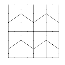
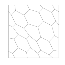
We have used different families of meshes
and the refinement parameter used to label
each mesh is the number of elements on each edge (see Figure 1):
1.
: trapezoidal meshes which consist of partitions
of the domain into congruent trapezoids taking the
middle point of each edge as a new degree of freedom;
note that each element has 8 edges;
2.
: non-structured hexagonal meshes made of convex hexagons.
We recall that the Lamé coefficients of a material are defined in
terms of the Young modulus and the Poisson ratio as follows:
and .
We have used the following physical parameters: density:
kg/m3, Young modulus:
Pa and Poisson ratio: .
We observe that the eigenfunctions of this problem may present singularities at the points
where the boundary condition changes from Dirichlet () to Neumann ().
According to [34], for , the estimate in Lemma 2.1(i)
holds true in this case for all .
Therefore, the theoretical order of convergence for the vibration frequencies
presented in Theorem 4.3 is
(see [37] for further details).
Figure 1: Sample meshes: and with , respectively.
We report in Table 1
the lowest vibration frequencies ,
computed with the method analyzed in this paper. The table also includes
estimated orders of convergence, as well as more accurate values of the
vibration frequencies extrapolated from the computed by means of
a least-squares fitting. Moreover, we compared our results with those
obtained in [37] with a stress-rotation mixed formulation
of the elasticity system and a mixed Galerkin method based on AFW element.
With this aim, we include in the last column of Table 1
the values obtained by extrapolating those reported in [37, Table 1].
Table 1: Test 1. Components lowest vibration frequencies , on different meshes.
It can be seen from Table 1
that the eigenvalue approximation order
of our method is quadratic and that the results
obtained by the two methods agree perfectly well.
Let us remark that the theoretical order of convergence
() is only a lower bound, since the actual order of
convergence for each vibration frequency depends on
the regularity of the corresponding eigenfunctions.
Therefore, the attained orders of convergence are in some cases
larger than this lower bound.
7.2 Test 2
The aim of this test is to assess the performance of the adaptive
scheme when solving a problem with a singular solution.
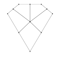
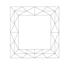
Let
which corresponds to a two-dimensional closed vessel with vacuum inside.
The boundary of the elastic body is the union of and : the solid is
fixed along and free of stress along ;
let the unit outward normal vector along
(see Figure 2).
Figure 2: Solid Domain.
We have used the following physical parameters: density: kg/m3,
Young modulus: Pa and Poisson ratio: .
In this numerical tests we have initiated the adaptive
process with a coarse triangular mesh. In order to compare the performance of
VEM with that of a the finite element method (FEM), we have used
two different algorithms to refine the meshes.
The first one is based on a classical FEM strategy for which all
the subsequent meshes consist of triangles. In such a case,
for , VEM reduces to FEM. The other procedure to refine the
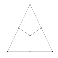
meshes is described in [13]. It consists of splitting
each element into quadrilaterals ( being the number of edges of the polygon) by connecting the
barycenter of the element with the midpoint of each edge as shown
in Figure 3 (see [13] for more details).
Notice that although this process is initiated with a mesh of triangles,
the successively created meshes will contain other kind of convex polygons as can be seen in Figure 5.
(a)Triangle refined into 3 quadrilaterals.
(b)Pentagon refined into 5 quadrilaterals.
Figure 3: Example of refined elements for VEM strategy.
We have used the two refinement procedures (VEM and FEM)
described above. Both schemes are based on the strategy of refining those elements which satisfy
Let us remark that in the case of triangular meshes, since
and hence and are the identity, the term
(see (6.2)) vanishes, by the same reason, the projection also disappears
in the definition (6.1) of and in (6.3)
reduces to .
The eigenfunctions of this problem may present singularities
at the points where the boundary condition changes from Dirichlet
() to Neumann () as well as at the reentrant angles of the domain
According to [34], in this case, the estimate in Lemma 2.1(i)
holds true in this case for all .
Therefore, in case of uniformly refined meshes,
the theoretical convergence rate for the eigenvalues should be
,
where denotes the number of degrees of freedom.
Now, an efficient adaptive scheme should lead to refine the meshes
in such a way that the optimal order
could be recovered.
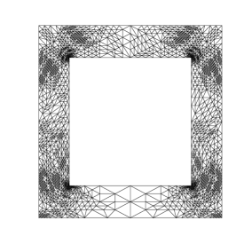
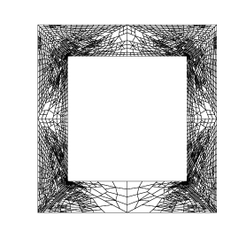
Figures 4 and 5 show the adaptively refined
meshes obtained with FEM and VEM procedures, respectively.
Figure 4: Adaptively refined meshes obtained whit FEM scheme at refinement steps 0, 1 and 8.
Figure 5: Adaptively refined meshes obtained whit VEM scheme at refinement steps 0, 1 and 8.
In order to compute the errors ,
due to the lack of an exact eigenvalue, we have used an approximation
based on a least squares fitting of the computed values obtained with
extremely refined meshes. Thus, we have obtained the value ,
which has at least four correct significant digits.
We report in Table 2 the lowest vibration frequency
on uniformly refined meshes and adaptive refined meshes
with FEM and VEM schemes. Each table includes the estimated convergence rate.
Table 2: Test 2. frequency computed with different schemes: uniformly refined meshes (“Uniform FEM”), adaptively refined meshes with FEM (“Adaptive FEM”) and adaptively refined meshes with VEM (“Adaptive VEM”).
Uniform FEM
Adaptative FEM
Adaptative VEM
136
0.2095
136
0.2095
136
0.2095
390
0.1758
300
0.1810
340
0.1718
1418
0.1625
806
0.1659
646
0.1626
5366
0.1567
1806
0.1599
1498
0.1574
20642
0.1551
2946
0.1577
2942
0.1557
80982
0.1543
4198
0.1563
4788
0.1550
6348
0.1554
7782
0.1545
9000
0.1549
12530
0.1543
12894
0.1545
19398
0.1541
18244
0.1543
26760
0.1541
Order
Order
Order
0.1538
0.1538
0.1538
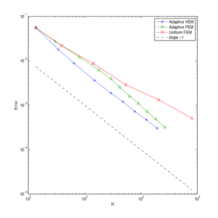
Figure 6: Test2. Error curves of for uniformly refined meshes
(“Uniform FEM”), adaptively refined meshes with
FEM (“Adaptive FEM”) and adaptively refined meshes with VEM (“Adaptive VEM”).
It can be seen from Figure 6 that the four refinement
schemes lead to the correct convergence rate. Moreover, the performance of adaptive VEM is slightly better than that of adaptive FEM.
We report in Table 3, the error
and the estimators at each step of the adaptative VEM scheme.
We include in the table the terms which arise from the inconsistency of VEM, which arise from the volumetric residuals and which arise from the edge residuals. We also report in the table the effectivity indexes .
Table 3: Test 2. Components of the error estimator and effectivity indexes on the adaptively refined meshes with VEM.
136
2.095e-01
5.570e-02
2.795e-05
0
1.643e-01
1.643e-01
3.390e-01
340
1.718e-01
1.797e-02
1.028e-05
2.244e-03
3.501e-02
3.726e-02
4.823e-01
646
1.626e-01
8.792e-03
4.353e-06
1.874e-03
1.777e-02
1.965e-02
4.475e-01
1498
1.574e-01
3.623e-03
2.520e-06
9.645e-04
7.441e-03
8.408e-03
4.309e-01
2942
1.557e-01
1.872e-03
1.039e-06
5.414e-04
4.348e-03
4.891e-03
3.827e-01
4788
1.550e-01
1.194e-03
6.433e-07
3.864e-04
2.883e-03
3.270e-03
3.652e-01
7782
1.545e-01
7.216e-04
4.495e-07
2.472e-04
2.007e-03
2.255e-03
3.200e-01
12530
1.543e-01
4.712e-04
2.894e-07
1.682e-04
1.367e-03
1.536e-03
3.068e-01
19398
1.541e-01
3.030e-04
1.845e-07
1.155e-04
9.524e-04
1.068e-03
2.837e-01
It can be seen from the Table 3 that the effectivity
indexes are bounded above and below far from zero and the inconsistency
and edge residual terms are roughly speaking of the same order,
none of them being asymptotically negliglible.
Acknowledgments
The first author was partially supported by CONICYT-Chile through
FONDECYT project 1140791 and by DIUBB through project 171508 GI/VC,
Universidad del Bío-Bío, (Chile).
The second author was partially supported by a CONICYT-Chile
through FONDECYT initiation project 111170534.
The authors are deeply grateful Prof. Rodolfo Rodríguez (Universidad de
Concepción) for the fruitful discussions.
References
[1]B. Ahmad, A. Alsaedi, F. Brezzi, L.D. Marini and A. Russo,
Equivalent projectors for virtual element methods,
Comput. Math. Appl., 66, (2013), pp. 376–391.
[2]M. Ainsworth and J.T. Oden,
A posteriori error estimation in finite element analysis,
In: Pure and Applied Mathematics. Wiley, New York (2000).
[3]P.F. Antonietti, L. Beirão da Veiga, D. Mora and M. Verani,
A stream virtual element formulation of the Stokes problem on polygonal meshes,
SIAM J. Numer. Anal., 52(1), (2014), pp. 386–404.
[4]P.F. Antonietti, L. Beirão da Veiga, S. Scacchi and M. Verani,
A virtual element method for the Cahn–Hilliard equation with polygonal meshes,
SIAM J. Numer. Anal., 54(1), (2016), pp. 36–56.
[5]I. Babuška and J. Osborn,
Eigenvalue problems,
in Handbook of Numerical Analysis, Vol. II,
P.G. Ciarlet and J.L. Lions, eds.,
North-Holland, Amsterdam, 1991, pp. 641–787.
[6]L. Beirão da Veiga, F. Brezzi, A. Cangiani, G. Manzini,
L.D. Marini and A. Russo,
Basic principles of virtual element methods,
Math. Models Methods Appl. Sci., 23, (2013), pp. 199–214.
[7]L. Beirão da Veiga, F. Brezzi and L.D. Marini,
Virtual elements for linear elasticity problems,
SIAM J. Numer. Anal., 51, (2013), pp. 794–812.
[8]L. Beirão da Veiga, F. Brezzi, L.D. Marini and A. Russo,
The hitchhiker’s guide to the virtual element method,
Math. Models Methods Appl. Sci., 24, (2014), pp. 1541–1573.
[9]L. Beirão da Veiga, F. Brezzi, L.D. Marini and A. Russo,
Virtual Element Method for general second-order
elliptic problems on polygonal meshes,
Math. Models Methods Appl. Sci., 26(4), (2016), pp. 729–750.
[10]L. Beirão da Veiga, K. Lipnikov and G. Manzini,
The Mimetic Finite Difference Method for Elliptic Problems,
Springer, MS&A, vol. 11, 2014.
[11]L. Beirão da Veiga, C. Lovadina and D. Mora,
A virtual element method for elastic and
inelastic problems on polytope meshes,
Comput. Methods Appl. Mech. Engrg., 295, (2015) pp. 327–346.
[12]L. Beirão da Veiga, C. Lovadina and G. Vacca,
Divergence free virtual elements for
the Stokes problem on polygonal meshes,
ESAIM Math. Model. Numer. Anal., 51(2), (2017) pp. 509–535.
[13]L. Beirão da Veiga and G. Manzini,
Residual a posteriori error estimation for the
virtual element method for elliptic problems,
ESAIM Math. Model. Numer. Anal., 49 (2015), pp. 577–599.
[14]L. Beirão da Veiga, D. Mora, G. Rivera and R. Rodríguez,
A virtual element method for the acoustic vibration problem,
Numer. Math., 136(3), (2017) pp. 725–763.
[15]L. Beirão da Veiga, D. Mora and G. Rivera,
Virtual elements for a shear-deflection
formulation of Reissner-Mindlin plates,
Math. Comp., DOI: https://doi.org/10.1090/mcom/3331 (2017).
[16]M.F. Benedetto, S. Berrone, A. Borio, S. Pieraccini, S. Scialò,
Order preserving SUPG stabilization for the virtual element
formulation of advection–diffusion problems,
Comput. Methods Appl. Mech. Engrg., 311, (2016), pp. 18–40.
[17]A. Bermúdez, P. Gamallo, L. Hervella-Nieto, R. Rodríguez and D. Santamarina,
Fluid-structure acoustic interaction.
Computational Acoustics of Noise Propagation in Fluids. Finite and Boundary Element Methods,
S. Marburg, B. Nolte, eds. Springer, 2008, Chap. 9, pp. 253–286.
[18]A. Bermúdez and R. Rodríguez,
Finite element computation of the vibration modes of a fluid-solid system,
Comput. Methods Appl. Mech. Engrg., 119(3-4), (1994), pp. 355–370.
[19]S. Berrone and A. Borio,
A residual a posteriori error estimate for the virtual element method,
Math. Models Methods Appl. Sci., 27, (2017), pp. 1423–1458.
[20]D. Boffi,
Finite element approximation of eigenvalue problems,
Acta Numerica, 19, (2010), pp. 1–120.
[21]D. Boffi, F. Gardini and L. Gastaldi,
Some remarks on eigenvalue approximation by finite elements,
in Frontiers in numerical analysis–Durham 2010,
Lect. Notes Comput. Sci. Eng., 85, Springer, Heidelberg, (2012), pp. 1–77.
[22]S.C. Brenner and R.L. Scott,
The Mathematical Theory of Finite Element Methods,
Springer, New York, 2008.
[23]F. Brezzi and L.D. Marini,
Virtual elements for plate bending problems,
Comput. Methods Appl. Mech. Engrg., 253, (2012), pp. 455–462.
[24]E. Cáceres and G.N. Gatica,
A mixed virtual element method for the pseudostress-velocity
formulation of the Stokes problem,
IMA J. Numer. Anal., 37(1), (2017) pp. 296–331.
[25]E. Cáceres, G.N. Gatica and F. Sequeira,
A mixed virtual element method
for the Brinkman problem,
Math. Models Methods Appl. Sci., 27(4), (2017) pp. 707–743.
[26]A. Cangiani, E.H. Georgoulis, T. Pryer and O.J. Sutton,
A posteriori error estimates for the virtual element method,
Numer. Math., 137(4), (2017) pp. 857–893.
[27]A. Cangiani, E.H. Georgoulis and P. Houston,
-version discontinuous Galerkin methods on polygonal and polyhedral meshes,
Math. Models Methods Appl. Sci., 24(10), (2014), pp. 2009–2041.
[28]C. Chinosi and L.D. Marini,
Virtual element method for fourth order problems: -estimates,
Comput. Math. Appl., 72(8), (2016), pp. 1959–1967.
[29]D. Di Pietro and A. Ern,
A hybrid high-order locking-free method for linear elasticity on general meshes,
Comput. Methods Appl. Mech. Eng., 283, (2015), pp. 1–21.
[30]D. Di Pietro and A. Ern,
Hybrid high-order methods for
variable-diffusion problems on general meshes,
C. R. Acad. Sci., Paris I, 353(1), (2015), pp. 31–34.
[31]A.L. Gain, C. Talischi and G.H. Paulino,
On the virtual element method for three-dimensional
linear elasticity problems on arbitrary polyhedral meshes,
Comput. Methods Appl. Mech. Engrg., 282, (2014), pp. 132–160.
[32]F. Gardini and G. Vacca,
Virtual element method for second order
elliptic eigenvalue problems,
IMA J. Numer. Anal., DOI: https://doi.org/10.1093/imanum/drx063 (2017).
[33]V. Girault and P.A. Raviart,
Finite Element Methods for Navier-Stokes Equations,
Springer-Verlag, Berlin, 1986.
[34]P. Grisvard,
Probléms aux limites dans les polygones. Mode démploi,
EDF, Bull. Dir. Etudes Rech. Ser. C, 1, (1986), pp. 21–59.
[35]E. Hernández,
Finite element approximation of the elasticity spectral problem on curved domains,
J. Comput. Appl. Math., 225, (2009), pp. 452–458.
[36]T. Kato,
Perturbation Theory for Linear Operators,
Springer Verlag, Berlin, 1995.
[37]S. Meddahi, D. Mora and R. Rodríguez,
Finite element spectral analysis for the mixed formulation of the elasticity equations,
SIAM J. Numer. Anal., 51(2), (2010), pp. 1041–1063.
[38]D. Mora, G. Rivera and R. Rodríguez,
A virtual element method for the Steklov eigenvalue problem,
Math. Models Methods Appl. Sci., 25(8), (2015), pp. 1421–1445.
[39]D. Mora, G. Rivera and R. Rodríguez,
A posteriori error estimates for a virtual element
method for the Steklov eigenvalue problem,
Comput. Math. Appl., 74(9), (2017), pp. 2172–2190.
[40]D. Mora, G. Rivera and I. Velásquez,
A virtual element method for the vibration problem of Kirchhoff plates,
ESAIM Math. Model. Numer. Anal., DOI: https://doi.org/10.1051/m2an/2017041 (2017).
[41]I. Perugia, P. Pietra and A. Russo,
A plane wave virtual element method for the Helmholtz problem,
ESAIM Math. Model. Numer. Anal., 50(3), (2016), pp. 783–808.
[42]N. Sukumar and A. Tabarraei,
Conforming polygonal finite elements,
Internat. J. Numer. Methods Engrg., 61, (2004), pp. 2045–2066.
[43]C. Talischi, G.H. Paulino, A. Pereira and I.F.M. Menezes,
Polygonal finite elements for topology optimization: A unifying paradigm,
Internat. J. Numer. Methods Engrg., 82(6), (2010), pp. 671–698.
[44]G. Vacca,
Virtual Element Methods for hyperbolic problems on polygonal meshes,
Comput. Math. Appl., 74(5), (2017), pp. 882–898.
[45]G. Vacca,
An -conforming virtual element for Darcy and Brinkman equations,
Math. Models Methods Appl. Sci., 28(1), (2018), pp. 159–194.
[46]G. Vacca and L. Beirão da Veiga,
Virtual element methods for parabolic problems on polygonal meshes,
Numer. Methods Partial Differential Equations, 31(6), (2015), pp. 2110–2134.
[47]R. Verfurth,
A review of a posteriori error estimate
and adaptative mesh-refinement techniques,
Wiley-Teubner, Chichester (1996).
[48]P. Wriggers, W.T. Rust and B.D. Reddy,
A virtual element method for contact,
Comput. Mech., 58, (2016), pp. 1039–1050.