Phylogenomics with Paralogs

Abstract.

Phylogenomics heavily relies on well-curated sequence data sets that consist, for each gene, exclusively of 1:1-orthologous. Paralogs are treated as a dangerous nuisance that has to be detected and removed. We show here that this severe restriction of the data sets is not necessary. Building upon recent advances in mathematical phylogenetics we demonstrate that gene duplications convey meaningful phylogenetic information and allow the inference of plausible phylogenetic trees, provided orthologs and paralogs can be distinguished with a degree of certainty. Starting from tree-free estimates of orthology, cograph editing can sufficiently reduce the noise in order to find correct event-annotated gene trees. The information of gene trees can then directly be translated into constraints on the species trees. While the resolution is very poor for individual gene families, we show that genome-wide data sets are sufficient to generate fully resolved phylogenetic trees, even in the presence of horizontal gene transfer.

We demonstrate that the distribution of paralogs in large gene families contains in itself sufficient phylogenetic signal to infer fully resolved species phylogenies. This source of phylogenetic information is independent of information contained in orthologous sequences and is resilient against horizontal gene transfer. An important consequence is that phylogenomics data sets need not be restricted to 1:1 orthologs.

1. Introduction

Molecular phylogenetics is primarily concerned with the reconstruction of evolutionary relationships between species based on sequence information. To this end, alignments of protein or DNA sequences are employed, whose evolutionary history is believed to be congruent to that of the respective species. This property can be ensured most easily in the absence of gene duplications and horizontal gene transfer. Phylogenetic studies judiciously select families of genes that rarely exhibit duplications (such as rRNAs, most ribosomal proteins, and many of the housekeeping enzymes). In phylogenomics, elaborate automatic pipelines such as HaMStR [Ebersberger:09], are used to filter genome-wide data sets to at least deplete sequences with detectable paralogs (homologs in the same species).

Figure 1. Outline of the computational framework. Starting from an estimated orthology relation $\Theta$, its graph representation $G_{\Theta}$ is edited to obtain the closest cograph $G_{\Theta^{*}}$, which in turn is equivalent to a (not necessarily fully resolved) gene tree $T$ and an event labeling $t$. From $(T,t)$ we extract the set $\mathbb{S}$ of all relevant species triples. As the triple set $\mathbb{S}$ need not to be consistent, we compute the maximal consistent subset $\mathbb{S^{*}}$ of $\mathbb{S}$. Finally, we construct a least resolved species tree from $\mathbb{S^{*}}$.

In the presence of gene duplications, however, it becomes necessary to distinguish between the evolutionary history of genes (gene trees) and the evolutionary history of the species (species trees) in which these genes reside. Leaves of a gene tree represent genes. Their inner nodes represent two kinds of evolutionary events, namely the duplication of genes within a genome – giving rise to paralogs – and speciations, in which the ancestral gene complement is transmitted to two daughter lineages. Two genes are (co-)orthologous if their last common ancestor in the gene tree represents a speciation event, while they are paralogous if their last common ancestor is a duplication event, see [Fitch2000] and [GK13] for a more recent discussion on orthology and paralogy relationships. Speciation events, in turn, define the inner vertices of a species tree. However, they depend on both, the gene and the species phylogeny, as well as the reconciliation between the two. The latter identifies speciation vertices in the gene tree with a particular speciation event in the species tree and places the gene duplication events on the edges of the species tree. Intriguingly, it is nevertheless possible in practice to distinguish orthologs with acceptable accuracy without constructing either gene or species trees [Altenhoff:09]. Many tools of this type have become available over the last decade, see [KWMK:11, DAAGD2013] for a recent review. The output of such methods is an estimate $\Theta$ of the true orthology relation $\Theta^{*}$, which can be interpreted as a graph $G_{\Theta}$ whose vertices are genes and whose edges connect estimated (co-)orthologs.

Recent advances in mathematical phylogenetics suggest that the estimated orthology relation $\Theta$ contains information on the structure of the species tree. To make this connection, we combine here three abstract mathematical results that are made precise in Materials and Methods below.

(1) Building upon the theory of symbolic ultrametrics [Boeckner:98] we showed that in the absence of horizontal gene transfer, the orthology relation of each gene family is a cograph [Hellmuth:13d]. Cographs can be generated from the single-vertex graph $K_{1}$ by complementation and disjoint union [Corneil:81]. This special structure of cographs imposes very strong constraints that can be used to reduce the noise and inaccuracies of empirical estimates of orthology from pairwise sequence comparison. To this end, the initial estimate of $G_{\Theta}$ is modified to the closest correct orthology relation $G_{\Theta^{*}}$ in such a way that a minimal number of edges (i.e., orthology assignments) are introduced or removed. This amounts to solving the cograph-editing problem [Liu:11, Liu:12].

(2) It is well known that each cograph is equivalently represented by its cotree [Corneil:81]. The cotree is easily computed for a given cograph. In our context, the cotree of $G_{\Theta^{*}}$ is an incompletely resolved event-labeled gene-tree. That is, in addition to the tree topology, we know for each internal branch point whether it corresponds to a speciation or a duplication event. Even though, adjacent speciations or adjacent duplications cannot be resolved, the tree faithfully encodes the relative order of any pair of duplication and speciation [Hellmuth:13d]. In the presence of horizontal gene transfer $G_{\Theta}$ may deviate from the structural requirements of a cograph. Still, the situation can be described in terms of edge-colored graphs whose subgraphs are cographs [Boeckner:98, Hellmuth:13d], so that the cograph structure remains an acceptable approximation.

(3) Every triple (rooted binary tree on three leaves) in the cotree that has leaves from three species and is rooted in a speciation event also appears in the underlying species tree [hernandez2012event]. Thus, the estimated orthology relation, after editing to a cograph and conversion to the equivalent event-labeled gene tree, provide many information on the species tree. This result allows us to collect from the cotrees for each gene family partial information on the underlying species tree. Interestingly, only gene families that harbor duplications, and thus have a non-trivial cotree, are informative. If no paralogs exist, then the orthology relation $G_{\Theta}$ is a clique (i.e., every family member is orthologous to every other family member) and the corresponding cotree is completely unresolved, and hence contains no triple. On the other hand, full resolution of the species tree is guaranteed if at least one duplication event between any two adjacent speciations is observable. The achievable resolution therefore depends on the frequency of gene duplications and the number of gene families.

Despite the variance reduction due to cograph editing, noise in the data, as well as the occasional introduction of contradictory triples as a consequence of horizontal gene transfer is unavoidable. The species triples collected from the individual gene families thus will not always be congruent. A conceptually elegant way to deal with such potentially conflicting information is provided by the theory of supertrees in the form of the largest set of consistent triples [Jansson:05, GM-13]. The data will not always contain a sufficient set of duplication events to achieve full resolution. To this end we consider trees with the property that the contraction of any edge leads to the loss of an input triple. There may be exponentially many alternative trees of this type. They can be listed efficiently using Semple’s algorithms [sem:03]. To reduce the solution space further we search for a least resolved tree in the sense of [Jansson:12], i.e., a tree that has the minimum number of inner vertices. It constitutes one of the best estimates of the phylogeny without pretending a higher resolution than actually supported by the data. In the Supplemental Material we discuss alternative choices.

The mathematical reasoning summarized above, outlined in Materials and Methods, and presented in full detail in the Supplemental Material, directly translates into a computational workflow, Fig. 1. It entails three NP-hard combinatorial optimization problems: cograph editing [Liu:12], maximal consistent triple set [Bryant97, Wu2004, Jansson2001] and least resolved supertree [Jansson:12]. We show here that they are nevertheless tractable in practice by formulating them as Integer Linear Programs (ILP) that can be solved for both, artificial benchmark data sets and real-life data sets, comprising genome-scale protein sets for dozens of species, even in the presence of horizontal gene transfer.

2. Preliminaries

Here, we summarize the definitions and notations required to outline the mathematical framework, presented in Section Theory and ILP Formulation

Phylogenetic Trees: We consider a set $\mathfrak{G}$ of at least three genes from a non-empty set $\mathfrak{S}$ of species. We denote genes by lowercase Roman and species by lowercase Greek letters. We assume that for each gene its species of origin is known. This is encoded by the surjective map $\sigma:\mathfrak{G}\to\mathfrak{S}$ with $a\mapsto\sigma(a)$. A phylogenetic tree (on $L$) is a rooted tree $T=(V,E)$ with leaf set $L\subseteq V$ such that no inner vertex $v\in V^{0}:=V\setminus L$ has outdegree one and whose root $\rho_{T}\in V$ has indegree zero. A phylogenetic tree $T$ is called binary if each inner vertex has outdegree two. A phylogenetic tree on $\mathfrak{G}$, resp., on $\mathfrak{S}$, is called gene tree, resp., species tree. A (inner) vertex $y$ is an ancestor of $x\in V$, in symbols $x\prec_{T}y$ if $y\neq x$ lies on the unique path connecting $x$ with $\rho_{T}$. The most recent common ancestor $\operatorname{lca}_{T}(L^{\prime})$ of a subset $L^{\prime}\subseteq L$ is the unique vertex in $T$ that is the least upper bound of $L^{\prime}$ under the partial order $\preceq_{T}$. We write $L(v):=\{y\in L|y\preceq_{T}v\}$ for the set of leaves in the subtree $T(v)$ of $T$ rooted in $v$. Thus, $L(\rho_{T})=L$ and $T(\rho_{T})=T$.

Rooted Triples: Rooted triples [Dress:book], i.e., rooted binary trees on three leaves, are a key concept in the theory of supertrees [sem-ste-03a, Bininda:book]. A rooted triple $r={\mathsf{(xy|z)}}$ with leaf set $L_{r}=\{x,y,z\}$ is displayed by a phylogenetic tree $T$ on $L$ if (i) $L_{r}\subseteq L$ and (ii) the path from $x$ to $y$ does not intersect the path from $z$ to the root $\rho_{T}$. Thus $\operatorname{lca}_{T}(x,y)\prec_{T}\operatorname{lca}_{T}(x,y,z)$. A set $R$ of triples is (strictly) dense on a given leaf set $L$ if for each set of three distinct leaves there is (exactly) one triple $r\in R$. We denote by $\mathfrak{R}(T)$ the set of all triples that are displayed by the phylogenetic tree $T$. A set $R$ of triples is consistent if there is a phylogenetic tree $T$ on $L_{R}:=\cup_{r\in R}L_{r}$ such that $R\subseteq\mathfrak{R}(T)$, i.e., $T$ displays (all triples of) $R$. If no such tree exists, $R$ is said to be inconsistent.
Given a triple set $R$, the polynomial-time algorithm BUILD [Aho:81] either constructs a phylogenetic tree $T$ displaying $R$ or recognizes that $R$ is inconsistent. The problem of finding a phylogenetic tree with the smallest possible number of vertices that is consistent with every rooted triple in $R$, i.e., a least resolved tree, is an NP-hard problem [Jansson:12]. If $R$ is inconsistent, the problem of determining a maximum consistent subset of an inconsistent set of triples is NP-hard and also APX-hard, see [Byrka:10a, vanIersel:09]. Polynomial-time approximation algorithms for this problem and further theoretical results are reviewed by [Byrka:10].

Triple Closure Operations and Inference Rules: If $R$ is consistent it is often possible to infer additional consistent triples. Denote by $\langle R\rangle$ the set of all phylogenetic trees on $L_{R}$ that display $R$. The closure of a consistent set of triples $R$ is $\displaystyle\operatorname{cl}(R)=\cap_{T\in\langle R\rangle}\mathfrak{R}(T)$, see [BS:95, GSS:07, Bryant97, huber2005recovering, BBDS:00]. We say $R$ is closed if $R=\operatorname{cl}(R)$ and write $R\vdash\mathsf{(xy|z)}$ iff $\mathsf{(xy|z)}\in\operatorname{cl}(R)$. The closure of a given consistent set $R$ can be computed in in $O(|R|^{5})$ time [BS:95]. Extending earlier work of Dekker [Dekker86], Bryant and Steel [BS:95] derived conditions under which $R\vdash\mathsf{(xy|z)}\implies R^{\prime}\vdash\mathsf{(xy|z)}$ for some $R^{\prime}\subseteq R$. Of particular importance are the following so-called 2-order inference rules:
          $\{\mathsf{(ab|c)},\mathsf{(ad|c)}\}\vdash\mathsf{(bd|c)}$ (i)
          $\{\mathsf{(ab|c)},\mathsf{(ad|b)}\}\vdash\mathsf{(bd|c)},\mathsf{(ad|c)}$ (ii)
          $\{\mathsf{(ab|c)},\mathsf{(cd|b)}\}\vdash\mathsf{(ab|d)},\mathsf{(cd|a)}$. (iii)
Inference rules based on pairs of triples $r_{1},r_{2}\in R$ can imply new triples only if $|L_{r_{1}}\cap L_{r_{2}}|=2$. Hence, in a strictly dense triple set only the three rules above may lead to new triples.

Cograph: Cographs have a simple characterization as $P_{4}$-free graphs, that is, no four vertices induce a simple path, although there are a number of equivalent characterizations, see [Brandstaedt:99]. Cographs can be recognized in linear time [Corneil:85, habib2005simple].

Orthology Relation: An empirical orthology relation $\Theta\subset\mathfrak{G}\times\mathfrak{G}$ is a symmetric, irreflexive relation that contains all pairs $(x,y)$ of orthologous genes. Here, we assume that $x,y\in\mathfrak{G}$ are paralogs if and only if $x\neq y$ and $(x,y)\notin\Theta$. This amounts to ignoring horizontal gene transfer. Orthology detection tools often report some weight or confidence value $w(x,y)$ for $x$ and $y$ to be orthologs from which $\Theta$ is estimated using a suitable cutoff. Importantly, $\Theta$ is symmetric, but not transitive, i.e., it does in general not represent a partition of $\mathfrak{G}$.

Event-Labeled Gene Tree: Given $\Theta$ we aim to find a gene tree $T$ with an “event labeling” $t:V^{0}\to\{\bullet,\square\}$ at the inner vertices so that, for any two distinct genes $x,y\in L$, $t(\operatorname{lca}_{T}(x,y))=\bullet$ if $\operatorname{lca}_{T}(x,y)$ corresponds to a speciation and hence $(x,y)\in\Theta$ and $t(\operatorname{lca}_{T}(x,y))=\square$ if $\operatorname{lca}_{T}(x,y)$ is a duplication vertex and hence $(x,y)\notin\Theta$. If such a tree $T$ with event-labeling $t$ exists for $\Theta$, we call the pair $(T,t)$ a symbolic representation of $\Theta$. We write $(T,t;\sigma)$ if in addition the species assignment map $\sigma$ is given. A detailed and more general introduction to the theory of symbolic representations is given in the Supplemental Material.

Reconciliation Map: A phylogenetic tree $S=(W,F)$ on $\mathfrak{S}$ is a species tree for a gene tree $T=(V,E)$ on $\mathfrak{G}$ if there is a reconciliation map $\mu:V\to W\cup F$ that maps genes $a\in\mathfrak{G}$ to species $\sigma(a)=\alpha\in\mathfrak{S}$ such that the ancestor relation $\preceq_{S}$ is implied by the ancestor relation $\preceq_{T}$. A more formal definition is given in the Supplemental Material. Inner vertices of $T$ that map to inner vertices of $S$ are speciations, while vertices of $T$ that map to edges of $S$ are duplications.

3. Theory

In this section, we summarize the main ideas and concepts behind our new methods that are based on our results established in [hernandez2012event, Hellmuth:13d]. We consider the following problem. Given an empirical orthology relation $\Theta$ we want to compute a species tree. To this end, four independent problems as explained below have to be solved.

From Estimated Orthologs to Cographs: Empirical estimates of the orthology relation $\Theta$ will in general contain errors in the form of false-positive orthology assignments, as well as false negatives, e.g., due to insufficient sequence similarity. Horizontal gene transfer adds to this noise. Hence an empirical relation $\Theta$ will in general not have a symbolic representation. In fact, $\Theta$ has a symbolic representation $(T,t)$ if and only if $G_{\Theta}$ is a cograph [Hellmuth:13d], from which $(T,t)$ can be derived in linear time, see also Theorem 4 in the Supplemental Material. However, the cograph editing problem, which aims to convert a given graph $G(V,E)$ into a cograph $G^{*}=(V,E^{*})$ with the minimal number $|E\vartriangle E^{*}|$ of inserted or deleted edges, is an NP-hard problem [Liu:11, Liu:12]. Here, the symbol $\vartriangle$ denotes the symmetric difference of two sets. In our setting the problem is considerably simplified by the structure of the input data. The gene set of every living organism consists of hundreds or even thousands of non-homologous gene families. Thus, the initial estimate of $G_{\Theta}$ already partitions into a large number of connected components. As shown in Lemma 9 in the Supplemental Material, it suffices to solve the cograph editing for each connected component separately.

Extraction of All Species Triples: From this edited cograph $G_{\Theta^{*}}$, we obtain a unique cotree that, in particular, is congruent to an incompletely resolved event-labeled gene-tree $(T,t;\sigma)$. In [hernandez2012event], we investigated the conditions for the existence of a reconciliation map $\mu$ from the gene tree $T$ to the species tree $S$. Given $(T,t;\sigma)$, consider the triple set $\mathbb{G}$ consisting of all triples $r=\mathsf{(ab|c)}\in\mathfrak{R}(T)$ so that (i) all genes $a,b,c$ belong to different species, and (ii) the event at the most recent common ancestor of $a,b,c$ is a speciation event, $t(\operatorname{lca}_{T}(a,b,c))=\bullet$. From $\mathbb{G}$ and $\sigma$, one can construct the following set of species triples:

$$\mathbb{S}=\left\{\mathsf{(\alpha\beta|\gamma)}|\,\exists\mathsf{(ab|c)}\in\mathbb{G}\textrm{\ with\ }\sigma(a)=\alpha,\sigma(b)=\beta,\sigma(c)=\gamma\right\}$$

The main result of [hernandez2012event] establishes that there is a species tree on $\sigma(\mathfrak{G})$ for $(T,t,\sigma)$ if and only if the triple set $\mathbb{S}$ is consistent. In this case, a reconciliation map can be found in polynomial time. No reconciliation map exists if $\mathbb{S}$ is inconsistent.

Maximal Consistent Triple Set: In practice, we cannot expect that the set $\mathbb{S}$ will be consistent. Therefore, we have to solve an NP-hard problem, namely, computing a maximum consistent subset of triples $\mathbb{S}^{*}\subset\mathbb{S}$ [Jansson:12]. The following result (see [GM-13] and Supplemental Material) plays a key role for the ILP formulation of triple consistency.

Theorem 1.

A strictly dense triple set $R$ on $L$ with $|L|\geq 3$ is consistent if and only if $\operatorname{cl}(R^{\prime})\subseteq R$ holds for all $R^{\prime}\subseteq R$ with $|R^{\prime}|=2$.

Least Resolved Species Tree: In order to compute an estimate for the species tree in practice, we finally compute from $\mathbb{S}^{*}$ a least resolved tree $S$ that minimizes the number of inner vertices. Hence, we have to solve another NP-hard problem [Byrka:10a, vanIersel:09]. However, some instances can be solved in polynomial time, which can be checked efficiently by utilizing the next result (see Supplemental Material).

Proposition 1.

If the tree $T$ inferred from the triple set $R$ by means of BUILD is binary, then the closure $\operatorname{cl}(R)$ is strictly dense. Moreover, $T$ is unique and hence, a least resolved tree for $R$.

4. ILP Formulation

Since we have to solve three intertwined NP-complete optimization problems we cannot realistically hope for an efficient exact algorithm. We therefore resort to ILP as the method of choice for solving the problem of computing a least resolved species tree $S$ from an empirical estimate of the orthology relation $G_{\Theta}$. We will use binary variables throughout. Table 1 summarizes the definition of the ILP variables and provides a key to the notation used in this section. In the following we summarize the ILP formulation. A detailed description and proofs for the correctness and completeness of the constraints can be found in the Supplemental Material.

Table 1. The notation used in the ILP formulation.

Sets & Constants	Definition
$\mathfrak{G}$	Set of genes
$\mathfrak{S}$	Set of species
$\Theta_{ab}$	Genes $a,b\in\mathfrak{G}$ are estimated orthologs:
	$\Theta_{ab}=1$ iff $(a,b)\in\Theta$.
Binary Variables	Definition
$E_{xy}$	Edge set of the cograph $G_{\Theta^{*}}=(\mathfrak{G},E_{\Theta^{*}})$
	of the closest relation $\Theta^{*}$ to $\Theta$:
	$E_{xy}=1$ iff $\{x,y\}\in E_{\Theta^{*}}$ (thus, iff $(x,y)\in\Theta^{*})$.
$T_{\mathsf{(\alpha\beta|\gamma)}}$	Rooted (species) triples in obtained set $\mathbb{S}$:
	$T_{\mathsf{(\alpha\beta|\gamma)}}=1$ iff $\mathsf{(\alpha\beta|\gamma)}\in\mathbb{S}$.
$T^{\prime}_{\mathsf{(\alpha\beta|\gamma)}}$, $T^{*}_{\mathsf{(\alpha\beta|\gamma)}}$	Rooted (species) triples in auxiliary strict dense
	set $\mathbb{S}^{\prime}$, resp., maximal consistent species triple
	set $\mathbb{S}^{*}$: $T^{\bullet}_{\mathsf{(\alpha\beta|\gamma)}}=1$ iff $\mathsf{(\alpha\beta|\gamma)}\in\mathbb{S}^{\bullet}$, $\bullet\in\{\prime,\ast\}$.
$M_{\alpha p}$	Set of clusters: $M_{\alpha p}=1$ iff $\alpha\in\mathfrak{S}$ is contained
	in cluster $p\in\{1,\dots,|\mathfrak{S}|-2\}$.
$N_{\alpha\beta,p}$	Cluster $p$ contains both species $\alpha$ and $\beta$:
	$N_{\alpha\beta,p}=1$ iff $M_{\alpha p}=1$ and $M_{\beta p}=1$
$C_{p,q,\Gamma\Lambda}$	Compatibility: $C_{p,q,\Gamma\Lambda}=1$ iff cluster $p$ and $q$
	have gamete $\Gamma\Lambda\in\{01,10,11\}$.
$Y_{p}$	Non-trivial clusters: $Y_{p}$=1 iff cluster $p\neq\emptyset$.

From Estimated Orthologs to Cographs: Our first task is to compute a cograph $G_{\Theta^{*}}$ that is as similar as possible to $G_{\Theta}$ (Eq. (1) and (1)) with the additional constraint that no pair of genes within the same species is connected by an edge, since no pair of orthologs can be found in the same species (Eq. (1)). Binary variables $E_{xy}$ express (non)edges in $G_{\Theta^{*}}$ and binary constants $\Theta_{ab}$ (non)pairs of the input relation $\Theta$. This ILP formulation requires $O(|\mathfrak{G}|^{2})$ binary variables and $O(|\mathfrak{G}|^{4})$ constraints. In practice, the effort is not dominated by the number of vertices, since the connected components of $G_{\Theta}$ can be treated independently.

Δ min& ∑_(x,y)∈$\mathfrak{G}$×$\mathfrak{G}$ (1-Θ_xy) E_xy + ∑_(x,y)∈$\mathfrak{G}$×$\mathfrak{G}$ Θ_xy (1-E_xy) Δ E_xy=0 for all x,y∈$\mathfrak{G}$ with σ(x)=σ(y) Δ &E_wx + E_xy+ E_yz - E_xz - E_wy - E_wz ≤2
∀ ordered tuples  (w,x,y,z)  of distinct  w,x,y,z∈$\mathfrak{G}$

Extraction of All Species Triples: The construction of the species tree $S$ is based upon the set $\mathbb{S}$ of species triples that can be derived from the set of gene triples $\mathbb{G}$, as explained in the previous section. Although the problem of determining such triples is not NP-hard, we give in the Supplemental Material an ILP formulation due to the sake of completeness. However, as any other approach can be used to determine the species triples we omit here the ILP formulation, but state that it requires $O(|\mathfrak{S}|^{3})$ variables and $O(|\mathfrak{G}|^{3}+|\mathfrak{S}|^{4})$ constraints.

Maximal Consistent Triple Set: An ILP approach to find maximal consistent triple sets was proposed in [chang2011ilp]. It explicitly builds up a binary tree as a way of checking consistency. Their approach, however, requires $O(|\mathfrak{S}|^{4})$ ILP variables, which limits the applicability in practice. By Theorem 1, strictly a dense triple set $R$ is consistent, if for all two-element subsets $R^{\prime}\subseteq R$ the closure $\operatorname{cl}(R^{\prime})$ is contained in $R$. This observation allows us to avoid the explicit tree construction and makes is much easier to find a maximal consistent subset $\mathbb{S}^{*}\subseteq\mathbb{S}$. Of course, neither $\mathbb{S}^{*}$ nor $\mathbb{S}$ need to be strictly dense. However, since $\mathbb{S}^{*}$ is consistent, Lemma 7 (Supplemental Material) guarantees that there is a strictly dense triple set $\mathbb{S}^{\prime}$ containing $\mathbb{S}^{*}$. Thus we have $\mathbb{S}^{*}=\mathbb{S}^{\prime}\cap\mathbb{S}$, where $\mathbb{S}^{\prime}$ must be chosen to maximize $|\mathbb{S}^{\prime}\cap\mathbb{S}|$. We define binary variables $T^{\prime}_{\mathsf{(\alpha\beta|\gamma)}}$, $T^{*}_{\mathsf{(\alpha\beta|\gamma)}}$, resp., binary constants $T_{\mathsf{(\alpha\beta|\gamma)}}$ to indicate whether $\mathsf{(\alpha\beta|\gamma)}$ is contained in $\mathbb{S}^{\prime}$, $\mathbb{S}^{*}$, resp., $\mathbb{S}$. The ILP formulation that uses $O(|\mathfrak{S}|^{3})$ variables and $O(|\mathfrak{S}|^{4})$ constraints is as follows. Δ max∑_$\mathsf{(\alpha\beta|\gamma)}$∈S T’_$\mathsf{(\alpha\beta|\gamma)}$ Δ &T’_$\mathsf{(\alpha\beta|\gamma)}$ + T’_$\mathsf{(\alpha\gamma|\beta)}$ + T’_$\mathsf{(\beta\gamma|\alpha)}$ = 1 Δ 2 T’_$\mathsf{(\alpha\beta|\gamma)}$ + 2&T’_$\mathsf{(\alpha\delta|\beta)}$ - T’_$\mathsf{(\beta\delta|\gamma)}$ - T’_$\mathsf{\mathsf{(\alpha\delta|\gamma)}}$ ≤2 Δ 0 ≤T’_$\mathsf{(\alpha\beta|\gamma)}$ + T_$\mathsf{(\alpha\beta|\gamma)}$ - 2T^*_$\mathsf{(\alpha\beta|\gamma)}$ ≤1 This ILP formulation can easily be adapted to solve a “weighted” maximum consistent subset problem: Denote by $w\mathsf{(\alpha\beta|\gamma)}$ the number of connected components in $G_{\Theta^{*}}$ that contain three vertices $a,b,c\in\mathfrak{G}$ with $\mathsf{(ab|c)}\in\mathbb{G}$ and $\sigma(a)=\alpha,\sigma(b)=\beta,\sigma(c)=\gamma$. These weights can simply be inserted into the objective function Eq. (1)

Δ max∑_$\mathsf{(\alpha\beta|\gamma)}$∈S T’_$\mathsf{(\alpha\beta|\gamma)}$*w$\mathsf{(\alpha\beta|\gamma)}$ to increase the relative importance of species triples in $\mathbb{S}$, if they are observed in multiple gene families.

Least Resolved Species Tree: We finally have to find a least resolved species tree from the set $\mathbb{S}^{*}$ computed in the previous step. Thus the variables $T^{*}_{\mathsf{(\alpha\beta|\gamma)}}$ become the input constants. For the explicit construction of the tree we use some of the ideas of [chang2011ilp]. To build an arbitrary tree for the consistent triple set $\mathbb{S}^{*}$, one can use one of the fast implementations of BUILD [sem-ste-03a]. If this tree is binary, then Proposition 1 implies that the closure $\operatorname{cl}(\mathbb{S}^{*})$ is strictly dense and that this tree is a unique and least resolved tree for $\mathbb{S}^{*}$. Hence, as a preprocessing step BUILD is used in advance, to test whether the tree for $\mathbb{S}^{*}$ is already binary. If not, we proceed with the following ILP approach that uses $O(|\mathfrak{S}|^{3})$ variables and constraints. Δ min &∑_p Y_p Δ 0 ≤Y_p—$\mathfrak{S}$— - ∑_α∈$\mathfrak{S}$ M_αp≤—$\mathfrak{S}$—-1 Δ 0≤& M_αp + M_βp - 2 N_αβ, p ≤1 Δ 1 - —$\mathfrak{S}$—(1- T^*_$\mathsf{(\alpha\beta|\gamma)}$) ≤∑_p N_αβ,p - 12 N_αγ,p -12 N_βγ,p Δ C_p,q,01≥&-M_αp+M_αq
C_p,q,10≥    M_αp-M_αq
C_p,q,11≥    M_αp+M_αq-1 Δ C_p,q,01 + C_p,q,10 + C_p,q,11 ≤2  ∀p,q Since a phylogenetic tree $S$ is equivalently specified by its hierarchy $\mathcal{C}=\{L(v)\mid v\in V(S)\}$ whose elements are called clusters (see Supplemental Material or [sem-ste-03a]), we construct the clusters induced by all triples of $\mathbb{S}^{*}$ and check whether they form a hierarchy on $\mathfrak{S}$. Following [chang2011ilp], we define the binary $|\mathfrak{S}|\times(|\mathfrak{S}|-2)$ matrix $M$, whose entries $M_{\alpha p}=1$ indicates that species $\alpha$ is contained in cluster $p$, see Supplemental Material. The entries $M_{\alpha p}$ serve as ILP variables. In contrast to the work of [chang2011ilp], we allow trivial columns in $M$ in which all entries are $0$. Minimizing the number of non-trivial columns then yields a least resolved tree.

For any two distinct species $\alpha,\beta$ and all clusters $p$ we introduce binary variables $N_{\alpha\beta,p}$ that indicate whether two species $\alpha,\beta$ are both contained in the same cluster $p$ or not (Eq. (1)). To determine whether a triple $\mathsf{(\alpha\beta|\gamma)}$ is contained in $\mathbb{S}^{*}\subseteq\mathbb{S}$ and displayed by a tree, we need the constraint Eq. (1). Following, the ideas of Chang et al. we use the “three-gamete condition”. Eq. (1) and (1) ensures that $M$ defines a “partial” hierarchy (any two clusters satisfy $p\cap q\in\{p,q,\emptyset\}$) of compatible clusters. A detailed discussion how these conditions establish that $M$ encodes a “partial” hierarchy can be found in the Supplemental Material.

Our aim is to find a least resolved tree that displays all triples of $\mathbb{S}^{*}$. We use the $|\mathfrak{S}|-2$ binary variables $Y_{p}=1$ to indicate whether there are non-zero entries in column $p$ (Eq. (1)). Finally, Eq. (1) captures that the number of non-trivial columns in $M$, and thus the number of inner vertices in the respective tree, is minimized. In the Supplemental Material we also discuss an ILP formulation to find a tree that displays the minimum number of additional triples not contained in $\mathbb{S}^{*}$ as an alternative to minimizing number of interior vertices.

5. Implementation and Data Sets

Details on implementation and test data sets can be found in the Supplemental Material. Simulated data were computed with and without horizontal gene transfer using both, the method described in [HHW+14] and the Artificial Life Framework (ALF) [Dalquen:12]. As real-life data sets we used the complete protein complements of 11 Aquificales and 19 Enterobacteriales species. The initial orthology relations are estimated with Proteinortho [Lechner:11a]. The ILP formulation of Fig. 1 is implemented in the Software ParaPhylo using IBM ILOG CPLEX™ Optimizer 12.6. ParaPhylo is freely available from
http://pacosy.informatik.uni-leipzig.de/paraphylo.

6. Results and Discussion

Figure 2. Accuracy of reconstructed species trees in simulated data sets. (a) Dependence on the number of gene families: 10 (left), and 20 (right) species and 100 to 500 gene families are generated using ALF with duplication/loss rate 0.005 and horizontal gene transfer rate $0.0$. (b) Dependence on the intensity of horizontal gene transfer: Orthology estimated with Proteinortho (left), and assuming perfect paralogy knowledge (right); $10$ species and $1000$ gene families are generated using ALF with duplication/loss rate $0.005$ and horizontal gene transfer rate ranging from $0.0$ to $0.0075$. (c) Dependence on the type and intensity ($p=5-25\%$) of noise in the raw orthology data $\Theta$: $10$ species and 1000 gene families are generated using ALF with duplication/loss rate $0.005$ and horizontal gene transfer rate $0.0$. Tree distances are measured by the triple metric (TT); all box plots summarize 100 independent data sets.

We have shown rigorously that orthology information alone is sufficient to reconstruct the species tree provided that (i) the orthology is known without error and unperturbed by horizontal gene transfer, and (ii) the input data contains a sufficient number of duplication events. While this species tree can be inferred in polynomial time for noise-free data, in a realistic setting three NP-hard optimization problems need to be solved.

To this end, we use here an exact ILP formulation implementing the workflow of Fig. 1 to compute species trees from empirically estimated orthology assignments. We first use simulated data to demonstrate that it is indeed feasible in practice to obtain correct gene trees directly from empirical estimates of orthology. For 5, 10, 15, and 20 species we obtained prefect, fully resolved reconstructions of 80%, 56%, 24%, and 11% of the species trees using 500 gene families. This comes with no surprise, given the low amount of paralogs in the simulations (7.5% to 11.2%), and the high amount of extremely short branches in the generated species trees – on 11.3% to 17.9% of the branches, less then one duplication is expected to occur. Nevertheless, the average TT distance was always smaller than 0.09 for more than 300 gene families, independent from the number of species, Fig. 2(a). Similar results for other tree distance measures are compiled in the Supplemental Material. Thus, deviations from perfect reconstructions are nearly exclusively explained by a lack of perfect resolution.

In order to evaluate the robustness of the species trees in response to noise in the input data we used simulated gene families with different noise models and levels: (i) insertion and deletion of edges in the orthology graph (homologous noise), (ii) insertion of edges (orthologous noise), (iii) deletion of edges (paralogous noise), and (iv) modification of gene/species assignments (xenologous noise). We observe a substantial dependence of the accuracy of the reconstructed species trees on the noise model. The results are most resilient against overprediction of orthology (noise model ii), while missing edges in $\Theta$ have a larger impact, see Fig. 2(c) for TT distance, and Supplemental Material for the other distances. This behavior can be explained by the observation that many false orthologs (overpredicting orthology) lead to an orthology graph, whose components are more clique-like and hence, yield few informative triples. Incorrect species triples thus are reduced, while missing species triples often can be supplemented through other gene families. On the other hand, if there are many false paralogs (underpredicting orthology) more false species triples are introduced, resulting in inaccurate trees. Xenologous noise (model iv), simulated by changing gene/species associations with probability $p$ while retaining the original gene tree, amounts to an extreme model for horizontal transfer. Our model, in particular in the weighted version, is quite robust for small amounts of HGT of 5% to 10%. Although some incorrect triples are introduced in the wake of horizontal transfer, they are usually dominated by correct alternatives observed from multiple gene families, and thus, excluded during computation of the maximal consistent triple set. Only large scale concerted horizontal transfer, which may occur in long-term endosymbiotic associations [Keeling:08], thus pose a serious problem.

Simulations with ALF[Dalquen:12] show that our method is resilient against errors resulting from mis-predicting xenology as orthology, see Fig. 2(b) right, even at horizontal gene transfer rates of $39.5\%$. Assuming perfect paralogy knowledge, i.e., assuming that all xenologs are mis-predicted as orthologs, the correct trees are reconstructed essentially independently from the amount of HGT for $69.75\%$ of the data sets, and the triple distance to the correct tree remain minute in the remaining cases. This is consistent with noise model (ii), i.e., a bias towards overpredicting orthology. Tree reconstruction based directly on the estimated orthology relation computed with Proteinortho are of course more inaccurate, Fig. 2(b) left. Even extreme rates of HGT, however, have no discernible effect on the quality of the inferred species trees. Our approach is therefore limited only by quality of initial orthology prediction tools.

The fraction $s$ of all triples obtained from the orthology relations that are retained in the final tree estimates serves as a quality measure similar in flavor e.g. to the retention index of cladistics. Bootstrapping support values for individual nodes are readily computed by resampling either at the level of gene families or at the level of triples (see Supplemental Material).

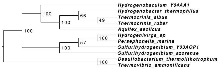
Figure 3. Phylogenetic tree of eleven Aquificales species inferred from paralogy. Internal node labels indicate triple-based bootstrap support.

For the Aquificales data set Proteinortho predicts 2856 gene families, from which 850 contain duplications. The reconstructed species tree (see Fig. 3, support $s=0.61$) is almost identical to the tree presented in [Lechner:14b]. All species are clustered correctly according to their taxonomic families. A slight difference refers to the two Sulfurihydrogenibium species not being directly clustered. These two species are very closely related. With only a few duplicates exclusively found in one of the species, the data was not sufficient for the approach to resolve this subtree correctly. Additionally, Hydrogenivirga sp. is misplaced next to Persephonella marina. This does not come as a surprise: Lechner et al. [Lechner:14b] already suspected that the data from this species was contaminated with material from Hydrogenothermaceae.

The second data set comprises the genomes of 19 Enterobacteriales with 8218 gene families of which 15 consists of more than 50 genes and 1342 containing duplications. Our orthology-based tree shows the expected groupings of Escherichia and Shigella species and identifies the monophyletic groups comprising Salmonella, Klebsiella, and Yersinia species. The topology of the deeper nodes agrees only in part with the reference tree from PATRIC database [Wattam:13], see Supplemental Material for additional information. The resulting tree has a support of $0.53$, reflecting that a few of the deeper nodes are poorly supported.

Data sets of around 20 species with a few thousand gene families, each having up to 50 genes, can be processed in reasonable time, see Table LABEL:tab:runtimeExtended. However, depending on the amount of noise in the data, the runtime for cograph editing can increase dramatically even for families with less than 50 genes.

7. Conclusion

We have shown here both theoretically and in a practical implementation that it is possible to access the phylogenetic information implicitly contained in gene duplications and thus to reconstruct a species phylogeny from information of paralogy only. This source of information is strictly complementary to the sources of information employed in phylogenomics studies, which are always based on alignments of orthologous sequences. In fact, 1:1 orthologs – the preferred data in sequence-based phylogenetics – correspond to cographs that are complete and hence have a star as their cotree and therefore do not contribute at all to the phylogenetic reconstruction in our approach. Access to the phylogenetic information implicit in (co-)orthology data requires the solution of three NP-complete combinatorial optimization problems. This is generally the case in phylogenetics, however: both the multiple sequence alignment problem and the extraction of maximum parsimony, maximum likelihood, or optimal Bayesian trees is NP-complete as well. Here we solve the computational tasks exactly for moderate-size problems by means of an ILP formulation. Using phylogenomic data for Aquificales and Enterobacteriales we demonstrated that non-trivial phylogenies can indeed be re-constructed from tree-free orthology estimates alone. Just as sequence-based approaches in molecular phylogeny crucially depend on the quality of multiple sequence alignments, our approach is sensitive to the initial estimate $\Theta$ of the orthology relation. Horizontal gene transfer, furthermore, is currently not included in the model but rather treated as noise that disturbs the phylogenetic signal. Simulated data indicate that the method is rather robust and can tolerate surprisingly large levels of noise in the form of both, mis-predicted orthology and horizontal gene transfer, provided a sufficient number of independent gene families is available as input data. Importantly, horizontal gene-transfer can introduce a bias only when many gene families are simultaneously affected by horizontal transfer. Lack of duplications, on the other hand, limits our resolution at very short time scales, a regime in which sequence-based approaches work very accurately.

We have used here an exact implementation as ILP to demonstrate the potential of the approach without confounding it with computational approximations. Thus, the current implementation does not easily scale to very large data sets. Paralleling the developments in sequence-based phylogenetics, where the NP-complete problems of finding a good input alignment and of constructing tree(s) maximizing the parsimony score, likelihood, or Bayesian posterior probability also cannot be solved exactly for large data sets, it will be necessary in practice to settle for heuristic solutions. In sequence-based phylogenetics, these have improved over decades to the point where they are no longer a limiting factor in phylogenetic reconstruction. Several polynomial time heuristics and approximation algorithms have been devised already for the triple consistency problem [Gasieniec:99, Maemura:07, Byrka:10a, Tazehkand:13]. The cograph editing problem and the least resolved tree problem, in contrast, have received comparably little attention so far, but constitute the most obvious avenues for boosting computational efficiency. Empirical observations such as the resilience of our approach against overprediction of orthologs in the input will certainly be helpful in designing efficient heuristics.

In the long run, we envision that the species tree $S$, and the symbolic representation of the event-annotated gene tree $(T,t)$ may serve as constraints for a refinement of the initial estimate of $\Theta$, solely making use only of (nearly) unambiguously identified branchings and event assignments. A series of iterative improvements of estimates for $\Theta$, $(T,t)$, and $S$, and, more importantly, methods that allow to accurately detect paralogs, may not only lead to more accurate trees and orthology assignments, but could also turn out to be computationally more efficient.

APPENDIX

8. Theory

In this section we give an expanded and more technical account of the mathematical theory underlying the relationships between orthology relations, triple sets, and the reconciliation of gene and triple sets. In particular, we include here the proofs of the key novel results outline in the main text. The notation in the main text is a subset of the one used here. Theorems, remarks, and ILP formulations have the same numbers as in the main text. As a consequence, the numberings in this supplement may not always be in ascending order.

8.1. Notation

For an arbitrary set $X$ we denote with $\binom{X}{n}$ the set of $n$-elementary subsets of X. In the remainder of this paper, $L$ will always denote a finite set of size at least three. Furthermore, we will denote with $\mathfrak{G}$ a set of genes and with $\mathfrak{S}$ a set of species and assume that $|\mathfrak{G}|\geq 3$ and $|\mathfrak{S}|\geq 1$. Genes contained in $\mathfrak{G}$ are denoted by lowercase Roman letters $a,b,c,\ldots$ and species in $\mathfrak{S}$ by lower case Greek letters $\alpha,\beta,\gamma\ldots$. Furthermore, let $\sigma:\mathfrak{G}\to\mathfrak{S}$ with $x\mapsto\sigma(x)$ be a mapping that assigns to each gene $x\in\mathfrak{G}$ its corresponding species $\sigma(x)=\chi\in\mathfrak{S}$. With $\sigma(\mathfrak{G})$ we denote the image of $\sigma$. W.l.o.g. we can assume that the map $\sigma$ is surjective, and thus, $\sigma(\mathfrak{G})=\mathfrak{S}$. We assume that the reader is familiar with graphs and its terminology, and refer to [Diestel12] as a standard reference.

8.2. Phylogenetic Trees

A tree $T=(V,E)$ is a connected cycle-free graph with vertex set $V(T)=V$ and edge set $E(T)=E$. A vertex of $T$ of degree one is called a leaf of $T$ and all other vertices of $T$ are called inner vertices. An edge of $T$ is an inner edge if both of its end vertices are inner vertices. The sets of inner vertices of $T$ is denoted by $V^{0}$. A tree $T$ is called binary if each inner vertex has outdegree two. A rooted tree $T=(V,E)$ is a tree that contains a distinguished vertex $\rho_{T}\in V$ called the root.

A phylogenetic tree $T$ (on $L$) is a rooted tree $T=(V,E)$ with leaf set $L\subseteq V$ such that no inner vertex has in- and outdegree one and whose root $\rho_{T}\in V$ has indegree zero. A phylogenetic tree on $\mathfrak{G}$, resp., on $\mathfrak{S}$, is called gene tree, resp., species tree.

Let $T=(V,E)$ be a phylogenetic tree on $L$ with root $\rho_{T}$. The ancestor relation $\preceq_{T}$ on $V$ is the partial order defined, for all $x,y\in V$, by $x\preceq_{T}y$ whenever $y$ lies on the (unique) path from $x$ to the root. Furthermore, we write $x\prec_{T}y$ if $x\preceq_{T}y$ and $x\neq y$. For a non-empty subset of leaves $L^{\prime}\subseteq L$, we define $\operatorname{lca}_{T}(L^{\prime})$, or the most recent common ancestor of $L^{\prime}$, to be the unique vertex in $T$ that is the least upper bound of $L^{\prime}$ under the partial order $\preceq_{T}$. In case $L^{\prime}=\{x,y\}$, we put $\operatorname{lca}_{T}(x,y):=\operatorname{lca}_{T}(\{x,y\})$ and if $L^{\prime}=\{x,y,z\}$, we put $\operatorname{lca}_{T}(x,y,z):=\operatorname{lca}_{T}(\{x,y,z\})$. If there is no danger of ambiguity, we will write $\operatorname{lca}(L^{\prime})$ rather then $\operatorname{lca}_{T}(L^{\prime})$.

For $v\in V$, we denote with $L(v):=\{y\in L|y\preceq_{T}v\}$ the set of leaves in the subtree $T(v)$ of $T$ rooted in $v$. Thus, $L(\rho_{T})=L$ and $T(\rho_{T})=T$.

It is well-known that there is a one-to-one correspondence between (isomorphism classes of) phylogenetic trees on $L$ and so-called hierarchies on $L$. For a finite set $L$, a hierarchy on $L$ is a subset $\mathcal{C}$ of the power set $\mathbb{P}(L)$ such that

1. $L\in\mathcal{C}$

2. $\{x\}\in\mathcal{C}$ for all $x\in L$ and

3. $p\cap q\in\{p,q,\emptyset\}$ for all $p,q\in\mathcal{C}$.

The elements of $\mathcal{C}$ are called clusters.  

Theorem 2 ([sem-ste-03a]).

Let $\mathcal{C}$ be a collection of non-empty subsets of $L$. Then, there is a phylogenetic tree $T$ on $L$ with $\mathcal{C}=\{L(v)\mid v\in V(T)\}$ if and only if $\mathcal{C}$ is a hierarchy on $L$.

The following result appears to be well known. We include a simple proof since we were unable to find a reference for it.  

Lemma 1.

The number of clusters $|\mathcal{C}|$ in a hierarchy $\mathcal{C}$ on $L$ determined by a phylogenetic tree $T=(V,E)$ on $L$ is bounded by $2|L|-1$.

Proof.

Clearly, the number of clusters $|\mathcal{C}|$ is determined by the number of vertices $|V|$, since each leaf $v\in L$, determines the singleton cluster $\{v\}\in\mathcal{C}$ and each inner node $v$ has at least two children and thus, gives rise to a new cluster $L(v)\in\mathcal{C}$. Hence, $|\mathcal{C}|=|V|$.

First, consider a binary phylogenetic tree $T=(V,E)$ on $|L|$ leaves. Then there are $|V|-|L|$ inner vertices, all of out-degree two. Hence, $|E|=2(|V|-|L|)=|V|-1$ and thus $|V|=2|L|-1$. Hence, $T$ determines $|\mathcal{C}|=2|L|-1$ clusters and has in particular $|L|-1$ inner vertices.

Now, its easy to verify by induction on the number of leaves $|L|$ that an arbitrary phylogenetic tree $T^{\prime}=(V^{\prime},E^{\prime})$ has $n_{0}\leq|L|-1$ inner vertices and thus, $|\mathcal{C}^{\prime}|=|V^{\prime}|=n_{0}+|L|\leq 2|L|-1$ clusters. ∎

8.3. Rooted Triples

8.3.1. Consistent Triple Sets

Rooted triples, sometimes also called rooted triplets [Dress:book], constitute an important concept in the context of supertree reconstruction [sem-ste-03a, Bininda:book] and will also play a major role here. A rooted triple $r={\mathsf{(xy|z)}}$ is displayed by a phylogenetic tree $T$ on $L$ if $x,y,z\in L$ pairwise distinct, and the path from $x$ to $y$ does not intersect the path from $z$ to the root $\rho_{T}$ and thus, having $\operatorname{lca}_{T}(x,y)\prec_{T}\operatorname{lca}_{T}(x,y,z)$. We denote with $L_{r}$ the set of the three leaves $\{x,y,z\}$ contained in the triple $r=\mathsf{(xy|z)}$, and with $L_{R}:=\cup_{r\in R}L_{r}$ the union of the leaf set of each $r\in R$. For a given leaf set $L$, a triple set $R$ is said to be (strict) dense if for each $x,y,z\in L$ there is (exactly) one triple $r\in R$ with $L_{r}=\{x,y,z\}$. For a phylogenetic tree $T$, we denote by $\mathfrak{R}(T)$ the set of all triples that are displayed by $T$. A set $R$ of triples is consistent if there is a phylogenetic tree $T$ on $L_{R}$ such that $R\subseteq\mathfrak{R}(T)$, i.e., $T$ displays all triples $r\in R$.

Not all sets of triples are consistent, of course. Given a triple set $R$ there is a polynomial-time algorithm, referred to in [sem-ste-03a] as BUILD, that either constructs a phylogenetic tree $T$ displaying $R$ or recognizes that $R$ is not consistent or inconsistent [Aho:81]. Various practical implementations have been described starting with [Aho:81], improved variants are discussed in [Henzinger:99, Jansson:05]. The problem of determining a maximum consistent subset of an inconsistent set of triples, however, is NP-hard and also APX-hard, see [Byrka:10a, vanIersel:09] and the references therein. We refer to [Byrka:10] for an overview on the available practical approaches and further theoretical results.

For a given consistent triple set $R$, a rooted phylogenetic tree, in which the contraction of any edge leads to the loss of an input triple is called a least resolved tree (for $R$). Following the idea of Janson et al. [Jansson:12], we are mainly concerned with the construction of least resolved trees, that have in addition as few inner vertices as possible and cover the largest subset of compatible triples contained in $R$. Finding a tree with a minimal number of inner nodes for a given consistent set of rooted triples is also an NP-hard problem, see [Jansson:12]. Unless stated explicitly, we use the term least resolved tree to refer to a tree with a minimum number of interior vertices, i.e., the least resolved trees in the sense of [Jansson:12]. Alternative choices include the trees that display the minimum number of additional triples not contained in $R$.

8.3.2. Graph Representation of Triples

There is a quite useful representation of a set of triples $R$ as a graph also known as Aho graph, see [Aho:81, huson2010phylogenetic, BS:95]. For given a triple set $R$ and an arbitrary subset $\mathcal{L}\subseteq L_{R}$, the graph $[R,\mathcal{L}]$ has vertex set $\mathcal{L}$ and two vertices $x,y\in\mathcal{L}$ are linked by an edge, if there is a triple $\mathsf{(xy|z)}\in R$ with $z\in\mathcal{L}$. Based on connectedness properties of the graph $[R,\mathcal{L}]$ for particular subsets $\mathcal{L}\subseteq L_{R}$, the algorithm BUILD recognizes if $R$ is consistent or not. In particular, this algorithm makes use of the following well-known theorem.

Theorem 3 ([Aho:81, BS:95]).

A set of rooted triples $R$ is consistent if and only if for each subset $\mathcal{L}\subseteq L_{R}$, $|\mathcal{L}|>1$ the graph $[R,\mathcal{L}]$ is disconnected.

Lemma 2 ([huson2010phylogenetic]).

Let $R$ be a dense set of rooted triples on $L$. Then for each $\mathcal{L}\subseteq L$, the number of connected components of the Aho graph $[R,\mathcal{L}]$ is at most two.

The tree computed with BUILD based on the Aho graph for a consistent set of rooted triples $R$ is denoted by $\mathrm{Aho}(R)$. Lemma 2 implies that $\mathrm{Aho}(R)$ must be binary for a consistent dense set of rooted triples. We will use the Aho graph and its key properties as a frequent tool in upcoming proofs.

For later reference, we recall

Lemma 3 ([BS:95]).

If $R^{\prime}$ is a subset of the triple set $R$ and $L$ is a leaf set, then $[R^{\prime},L]$ is a subgraph of $[R,L]$.

8.3.3. Closure Operations and Inference Rules

The requirement that a set $R$ of triples is consistent, and thus, that there is a tree displaying all triples, allows to infer new triples from the set of all trees displaying all triples of $R$ and to define a closure operation for $R$, which has been extensively studied in the last decades, see [BS:95, GSS:07, Bryant97, huber2005recovering, BBDS:00]. Let $\langle R\rangle$ be the set of all phylogenetic trees on $L_{R}$ that display all the triples of $R$. The closure of a consistent set of rooted triples $R$ is defined as

$$\operatorname{cl}(R)=\bigcap_{T\in\langle R\rangle}\mathfrak{R}(T).$$

This operation satisfies the usual three properties of a closure operator, namely: $R\subseteq\operatorname{cl}(R)$; $\operatorname{cl}(\operatorname{cl}(R))=\operatorname{cl}(R)$ and if $R^{\prime}\subseteq R$, then $\operatorname{cl}(R^{\prime})\subseteq\operatorname{cl}(R)$. We say $R$ is closed if $R=\operatorname{cl}(R)$. Clearly, for any tree $T$ it holds that $\mathfrak{R}(T)$ is closed. The brute force computation of the closure of a given consistent set $R$ runs in $O(|R|^{5})$ time [BS:95]: For any three leaves $x,y,z\in L_{R}$ test whether exactly one of the sets $R\cup\{\mathsf{(xy|z)}\}$, $R\cup\{\mathsf{(xz|y)}\}$, $R\cup\{\mathsf{(zy|x)}\}$ is consistent, and if so, add the respective triple to the closure $\operatorname{cl}(R)$ of $R$.

For a consistent set $R$ of rooted triples we write $R\vdash\mathsf{(xy|z)}$ if any phylogenetic tree that displays all triples of $R$ also displays $\mathsf{(xy|z)}$. In other words, $R\vdash\mathsf{(xy|z)}$ iff $\mathsf{(xy|z)}\in\operatorname{cl}(R)$. In a work of Bryant and Steel [BS:95], in which the authors extend and generalize the work of Dekker [Dekker86], it was shown under which conditions it is possible to infer triples by using only subsets $R^{\prime}\subseteq R$, i.e., under which conditions $R\vdash\mathsf{(xy|z)}\implies R^{\prime}\vdash\mathsf{(xy|z)}$ for some $R^{\prime}\subseteq R$. In particular, we will make frequent use of the following inference rules:

(i) $$\{\mathsf{(ab|c)},\mathsf{(ad|c)}\} \vdash\mathsf{(bd|c)}$$

(ii) $$\{\mathsf{(ab|c)},\mathsf{(ad|b)}\} \vdash\mathsf{(bd|c)},\mathsf{(ad|c)}$$

(iii) $$\{\mathsf{(ab|c)},\mathsf{(cd|b)}\} \vdash\mathsf{(ab|d)},\mathsf{(cd|a)}.$$

Remark 1.

It is an easy task to verify, that such inference rules based on two triples $r_{1},r_{2}\in R$ can lead only to new triples, whenever $|L_{r_{1}}\cap L_{r_{2}}|=2$. Hence, the latter three stated rules are the only ones that lead to new triples for a given pair of triples in a strictly dense triple set.

For later reference and the ILP formulation, we give the following lemma.

Lemma 4.

Let $R$ be a strictly dense set of rooted triples. For all $L^{\prime}=\{a,b,c,d\}\subseteq L_{R}$ we have the following statements:

All triples inferred by rule (ii) applied on triples $r\in R$ with $L_{r}\subset L^{\prime}$ are contained in $R$ if and only if all triples inferred by rule (iii) applied on triples $r\in R$ with $L_{r}\subset L^{\prime}$ are contained in $R$.

Moreover, if all triples inferred by rule (ii) applied on triples $r\in R$ with $L_{r}\subset L^{\prime}$ are contained in $R$ then all triples inferred by rule (i) applied on triples $r\in R$ with $L_{r}\subset L^{\prime}$ are contained in $R$.

Proof.

The first statement was established in [GM-13, Lemma 2].

For the second statement assume that for all pairwise distinct $L^{\prime}=\{a,b,c,d\}\subseteq L_{R}$ it holds that all triples inferred by rule (ii), or equivalently, by rule (iii) applied on triples $r\in R$ with $L_{r}\subset L^{\prime}$ are contained in $R$. Assume for contradiction that there are triples $\mathsf{(ab|c)},\mathsf{(ad|c)}\in R$, but $\mathsf{(bd|c)}\not\in R$. Since $R$ is strictly dense, we have either $\mathsf{(bc|d)}\in R$ or $\mathsf{(cd|b)}\in R$. In the first case and since $\mathsf{(ab|c)}\in R$, rule (ii) implies that $\mathsf{(ac|d)}\in R$, a contradiction. In the second case and since $\mathsf{(ab|c)}\in R$, rule (iii) implies that $\mathsf{(cd|a)}\in R$, a contradiction. ∎

We are now in the position to prove the following important and helpful lemmas and theorem. The final theorem basically states that consistent strict dense triple sets can be characterized by the closure of any two element subset of $R$. Note, an analogous result was established by [GM-13]. However, we give here an additional direct and transparent proof.

Lemma 5.

Let $R$ be a strictly dense set of triples on $L$ such that for all $R^{\prime}\subseteq R$ with $|R^{\prime}|=2$ it holds $\operatorname{cl}(R^{\prime})\subseteq R$. Let $x\in L$ and $L^{\prime}=L\setminus\{x\}$. Moreover, let $R_{|L^{\prime}}\subset R$ denote the subset of all triples $r\in R$ with $L_{r}\subseteq L^{\prime}$. Then $R_{|L^{\prime}}$ is strictly dense and for all $R^{\prime}\subseteq R_{|L^{\prime}}$ with $|R^{\prime}|=2$ it holds $\operatorname{cl}(R^{\prime})\subseteq R_{|L^{\prime}}$.

Proof.

Clearly, since $R$ is strictly dense and since $R_{|L^{\prime}}$ contains all triples except the ones containing $x$ it still holds that for all $a,b,c\in L^{\prime}$ there is exactly one triple $r\in R_{|L^{\prime}}$ with $a,b,c\in L_{r}$. Hence, $R_{|L^{\prime}}$ is strictly dense.

Assume for contradiction, that there are triples $r_{1},r_{2}\in R_{|L^{\prime}}\subset R$ with $\operatorname{cl}(r_{1},r_{2})\not\subseteq R_{|L^{\prime}}$. By construction of $R_{|L^{\prime}}$, no triples $r_{1},r_{2}\in R_{|L^{\prime}}$ can infer a new triple $r_{3}$ with $x\in L_{r_{3}}$. This immediately implies that $\operatorname{cl}(r_{1},r_{2})\not\subseteq R$, a contradiction. ∎

Lemma 6.

Let $R$ be a strictly dense set of triples on $L$ with $|L|=4$. If for all $R^{\prime}\subseteq R$ with $|R^{\prime}|=2$ holds $\operatorname{cl}(R^{\prime})\subseteq R$ then $R$ is consistent.

Proof.

By contraposition, assume that $R$ is not consistent. Thus, the Aho graph $[R,\mathcal{L}]$ is connected for some $\mathcal{L}\subseteq L$. Since $R$ is strict dense, for any $\mathcal{L}\subseteq L$ with $|\mathcal{L}|=2$ or $|\mathcal{L}|=3$ the Aho graph $[R,\mathcal{L}]$ is always disconnected. Hence, $[R,\mathcal{L}]$ for $\mathcal{L}=L$ must be connected. The graph $[R,L]$ has four vertices, say $a,\ b,\ c$ and $d$. The fact that $R$ is strictly dense and $|L|=4$ implies that $|R|=4$ and in particular, that $[R,L]$ has three or four edges. Hence, the graph $[R,L]$ is isomorphic to one of the following graphs $G_{0}$, $G_{1}$ or $G_{2}$.

The graph $G_{0}$ is isomorphic to a path $x_{1}-x_{2}-x_{3}-x_{4}$ on four vertices; $G_{1}$ is isomorphic to a chordless square; and $G_{2}$ is isomorphic to a path $x_{1}-x_{2}-x_{3}-x_{4}$ on four vertices where the edge $\{x_{1},x_{3}\}$ or $\{x_{2},x_{4}\}$ is added. W.l.o.g. assume that for the first case $[R,L]\simeq G_{0}$ has edges $\{a,b\}$, $\{b,c\}$, $\{c,d\}$; for the second case $[R,L]\simeq G_{1}$ has edges $\{a,b\}$, $\{a,c\}$, $\{c,d\}$ and $\{b,d\}$ and for the third case assume that $[R,L]\simeq G_{2}$ has edges $\{a,b\}$, $\{a,c\}$, $\{c,d\}$ and $\{a,d\}$.

Let $[R,L]\simeq G_{0}$. Then there are triples of the form $\mathsf{(ab|*)}$, $\mathsf{(bc|*)}$, $\mathsf{(cd|*)}$, where one kind of triple must occur twice, since otherwise, $[R,L]$ would have four edges. Assume that this is $\mathsf{(ab|*)}$. Hence, the triples $\mathsf{(ab|c)},\mathsf{(ab|d)}\in R$ since $|R|=4$. Since $R$ is strictly dense, $\mathsf{(bc|*)}=\mathsf{(bc|d)}\in R$, which implies that $\mathsf{(cd|*)}=\mathsf{(cd|a)}\in R$. Now, $R^{\prime}=\{\mathsf{(ab|c)},\mathsf{(bc|d)}\}\vdash\mathsf{(ac|d)}$. However, since $R$ is strictly dense and $\mathsf{(cd|a)}\in R$ we can conclude that $\mathsf{(ac|d)}\not\in R$, and therefore $\operatorname{cl}(R^{\prime})\not\subseteq R$. The case with triples $\mathsf{(cd|*)}$ occurring twice is treated analogously. If triples $\mathsf{(bc|*)}$ occur twice, we can argue the same way to obtain obtain $\mathsf{(bc|a)},\mathsf{(bc|d)}\in R$, $\mathsf{(ab|*)}=\mathsf{(ab|d)}$, and $\mathsf{(cd|*)}=\mathsf{(cd|a)}$. However, $R^{\prime}=\{\mathsf{(bc|a)},\mathsf{(cd|a)}\}\vdash\mathsf{(bd|a)}\notin R$, and thus $\operatorname{cl}(R^{\prime})\not\subseteq R$.

Let $[R,L]\simeq G_{1}$. Then there must be triples of the form $\mathsf{(ab|*)}$, $\mathsf{(ac|*)}$, $\mathsf{(cd|*)}$, $\mathsf{(bd|*)}$. Clearly, $\mathsf{(ab|*)}\in\{\mathsf{(ab|c)},\mathsf{(ab|d)}\}$. Note that not both $\mathsf{(ab|c)}$ and $\mathsf{(ab|d)}$ can be contained in $R$, since then $[R,L]\simeq G_{0}$. If $\mathsf{(ab|*)}=\mathsf{(ab|c)}$ and since $R$ is strict dense, $\mathsf{(ac|*)}=\mathsf{(ac|d)}$. Again, since $R$ is strictly dense, $\mathsf{(cd|*)}=\mathsf{(cd|b)}$ and this implies that $\mathsf{(bd|*)}=\mathsf{(bd|a)}$. However, $R^{\prime}=\{\mathsf{(ab|c)},\mathsf{(ac|d)}\}\vdash\mathsf{(ab|d)}\notin R$, since $R$ is strictly dense and $\mathsf{(bd|a)}\in R$. Thus, $\operatorname{cl}(R^{\prime})\not\subseteq R$. If $\mathsf{(ab|*)}=\mathsf{(ab|d)}$ and since $R$ is strictly dense, we can argue analogously, and obtain, $\mathsf{(bd|*)}=\mathsf{(bd|c)}$, $\mathsf{(cd|*)}=\mathsf{(cd|a)}$ and $\mathsf{(ac|*)}=\mathsf{(ac|b)}$. However, $R^{\prime}=\{\mathsf{(ab|d)},\mathsf{(bd|c)}\}\vdash\mathsf{(ad|c)}\notin R$, and thus $\operatorname{cl}(R^{\prime})\not\subseteq R$.

Let $[R,L]\simeq G_{2}$. Then there must be triples of the form $\mathsf{(ab|*)}$, $\mathsf{(ac|*)}$, $\mathsf{(cd|*)}$, $\mathsf{(ad|*)}$. Again, $\mathsf{(ab|*)}\in\{\mathsf{(ab|c)},\mathsf{(ab|d)}\}$. By similar arguments as in the latter two cases, if $\mathsf{(ab|*)}=\mathsf{(ab|c)}$ then we obtain, $\mathsf{(ac|*)}=\mathsf{(ac|d)}$, $\mathsf{(ad|*)}=\mathsf{(ad|b)}$ and $\mathsf{(cd|*)}=\mathsf{(cd|b)}$. Since $R^{\prime}=\{\mathsf{(ab|c)},\mathsf{(ac|d)}\}\vdash\mathsf{(bc|d)}\notin R$, we can conclude that $\operatorname{cl}(R^{\prime})\not\subseteq R$. If $\mathsf{(ab|*)}=\mathsf{(ab|d)}$ we obtain analogously, $\mathsf{(ad|*)}=\mathsf{(ad|c)}$, $\mathsf{(cd|*)}=\mathsf{(cd|b)}$ and $\mathsf{(ac|*)}=\mathsf{(ac|b)}$. However, $R^{\prime}=\{\mathsf{(ab|d)},\mathsf{(ad|c)}\}\vdash\mathsf{(bd|c)}\notin R$, and thus $\operatorname{cl}(R^{\prime})\not\subseteq R$. ∎

Theorem 1.

Let $R$ be a strictly dense triple set on $L$ with $|L|\geq 3$. The set $R$ is consistent if and only if $\operatorname{cl}(R^{\prime})\subseteq R$ holds for all $R^{\prime}\subseteq R$ with $|R^{\prime}|=2$.

Proof.

$\Rightarrow:$ If $R$ is strictly dense and consistent, then for any triple triple $\mathsf{(ab|c)}\notin R$ holds $R\cup\mathsf{(ab|c)}$ is inconsistent as either $\mathsf{(ac|b)}$ or $\mathsf{(bc|a)}$ is already contained in $R$. Hence, for each $a,b,c\in L$ exactly one $R\cup\{\mathsf{(ab|c)}\}$, $R\cup\{\mathsf{(ac|b)}\}$, $R\cup\{\mathsf{(bc|a)}\}$ is consistent, and this triple is already contained in $R$. Hence, $R$ is closed. Therefore, for any subset $R^{\prime}\subseteq R$ holds $\operatorname{cl}(R^{\prime})\subseteq\operatorname{cl}(R)=R$. In particular, this holds for all $R^{\prime}\subseteq R$ with $|R^{\prime}|=2$.

$\Leftarrow:$ (Induction on $|L|$.)
If $|L|=3$ and since $R$ is strictly dense, it holds $|R|=1$ and thus, $R$ is always consistent. If $|L|=4$, then Lemma 6 implies that if for any two-element subset $R^{\prime}\subseteq R$ holds that $\operatorname{cl}(R^{\prime})\subseteq R$, then $R$ is consistent. Assume therefore, the assumption is true for all strictly dense triple sets $R$ on $L$ with $|L|=n$.

Let $R$ be a strictly dense triple set on $L$ with $|L|=n+1$ such that for each $R^{\prime}\subseteq R$ with $|R^{\prime}|=2$ it holds $\operatorname{cl}(R^{\prime})\subseteq R$. Moreover, let $L^{\prime}=L\setminus\{x\}$ for some $x\in L$ and $R_{|L^{\prime}}\subset R$ denote the subset of all triples $r\in R$ with $L_{r}\subset L^{\prime}$. Lemma 5 implies that $R_{|L^{\prime}}$ is strictly dense and for each $R^{\prime}\subseteq R_{|L^{\prime}}$ with $|R^{\prime}|=2$ we have $\operatorname{cl}(R^{\prime})\subseteq R_{|L^{\prime}}$. Hence, the induction hypothesis can be applied for any such $R_{|L^{\prime}}$ implying that $R_{|L^{\prime}}$ is consistent. Moreover, since $R_{|L^{\prime}}$ is strictly dense and consistent, for any triple $\mathsf{(xy|z)}\notin R_{|L^{\prime}}$ holds that $R_{|L^{\prime}}\cup\mathsf{(xy|z)}$ is inconsistent. But this implies that $R_{|L^{\prime}}$ is closed, i.e., $\operatorname{cl}(R_{|L^{\prime}})=R_{|L^{\prime}}$. Lemma 2 implies that the Aho graph $[R_{|L^{\prime}},\mathcal{L}]$ has exactly two connected components $C_{1}$ and $C_{2}$ for each $\mathcal{L}\subseteq L^{\prime}$ with $|\mathcal{L}|>1$. In the following we denote with $\mathcal{L}_{i}=V(C_{i})$, $i=1,2$ the set of vertices of the connected component $C_{i}$ in $[R_{|L^{\prime}},\mathcal{L}]$. Clearly, $\mathcal{L}=\mathcal{L}_{1}\dot{\cup}\mathcal{L}_{2}$. It is easy to see that $[R,\mathcal{L}]\simeq[R_{|L^{\prime}},\mathcal{L}]$ for any $\mathcal{L}\subseteq L^{\prime}$, since none of the graphs contain vertex $x$. Hence, $[R,\mathcal{L}]$ is always disconnected for any $\mathcal{L}\subseteq L^{\prime}$. Therefore, it remains to show that, for all $\mathcal{L}\cup\{x\}$ with $\mathcal{L}\subseteq L^{\prime}$ holds: if for any $R^{\prime}\subseteq R$ with $|R^{\prime}|=2$ holds $\operatorname{cl}(R^{\prime})\subseteq R$, then $[R,\mathcal{L}\cup\{x\}]$ is disconnected and hence, $R$ is consistent.

To proof this statement we consider the different possibilities for $\mathcal{L}$ separately. We will frequently use that $[R_{|L^{\prime}},\mathcal{L}]$ is a subgraph of $[R,\mathcal{L}]$ for every $\mathcal{L}\subseteq L$ (Lemma 3).

Case 1. If $|\mathcal{L}|=1$, then $\mathcal{L}\cup\{x\}$ implies that $[R,\mathcal{L}\cup\{x\}]$ has exactly two vertices and clearly, no edge. Thus, $[R,\mathcal{L}\cup\{x\}]$ is disconnected.

Case 2. Let $|\mathcal{L}|=2$ with $\mathcal{L}_{1}=\{a\}$ and $\mathcal{L}_{2}=\{b\}$. Since $R$ is strictly dense, exactly one of the triples $\mathsf{(ab|x)}$, $\mathsf{(ax|b)}$, or $\mathsf{(xb|a)}$ is contained in $R$. Hence, $[R,\mathcal{L}\cup\{x\}]$ has exactly three vertices where two of them are linked by an edge. Thus, $[R,\mathcal{L}\cup\{x\}]$ is disconnected.

Case 3. Let $|\mathcal{L}|\geq 3$ with $\mathcal{L}_{1}=\{a_{1},\ldots,a_{n}\}$ and $\mathcal{L}_{2}=\{b_{1},\ldots,b_{m}\}$. Since $R_{|L^{\prime}}$ is consistent and strict dense and by construction of $\mathcal{L}_{1}$ and $\mathcal{L}_{2}$ it holds $\forall a_{i},a_{j}\in\mathcal{L}_{1},b_{k}\in\mathcal{L}_{2},i\neq j:\mathsf{(a_{i}a_{j}|b_{k})}\in R_{|L^{\prime}}\subseteq R$ and $\forall a_{i}\in\mathcal{L}_{1},b_{k},b_{l}\in\mathcal{L}_{2},k\neq l:\mathsf{(b_{k}b_{l}|a_{i})}\in R_{|L^{\prime}}\subseteq R$. Therefore, since $R$ is strictly dense, there cannot be any triple of the form $\mathsf{(a_{i}b_{k}|a_{j})}$ or $\mathsf{(a_{i}b_{k}|b_{l})}$ with $a_{i},a_{j}\in\mathcal{L}_{1},b_{k},b_{l}\in\mathcal{L}_{2}$ that is contained $R$. It remains to show that $R$ is consistent. The following three subcases can occur.

• The connected components $C_{1}$ and $C_{2}$ of $[R_{|L^{\prime}},\mathcal{L}]$ are connected in $[R,\mathcal{L}\cup\{x\}]$. Hence, there must be a triple $\mathsf{(ab|x)}\in R$ with $a\in\mathcal{L}_{1}$ and $b\in\mathcal{L}_{2}$. Hence, in order to prove that $R$ is consistent, we need to show that there is no triple $\mathsf{(cx|d)}$ contained $R$ for all $c,d\in\mathcal{L}$, which would imply that $[R,\mathcal{L}\cup\{x\}]$ stays disconnected.

• The connected component $C_{1}$ of $[R_{|L^{\prime}},\mathcal{L}]$ is connected to $x$ in $[R,\mathcal{L}\cup\{x\}]$. Hence, there must be a triple $\mathsf{(ax|c)}\in R$ with $a\in\mathcal{L}_{1}$, $c\in\mathcal{L}$. Hence, in order to prove that $R$ is consistent, we need to show that there are no triples $\mathsf{(b_{k}x|a_{i})}$ and $\mathsf{(b_{k}x|b_{l})}$ for all $a_{i}\in\mathcal{L}_{1}$, $b_{k},b_{l}\in\mathcal{L}_{2}$, which would imply that $[R,\mathcal{L}\cup\{x\}]$ stays disconnected.

• As in Case $3.b)$, the connected component $C_{2}$ of $[R_{|L^{\prime}},\mathcal{L}]$ might be connected to $x$ in $[R,\mathcal{L}\cup\{x\}]$ and we need to show that there are no triples $\mathsf{(a_{i}x|b_{k})}$ and $\mathsf{(a_{i}x|a_{j})}$$\mathsf{(a_{i}x|a_{j})}$ for all $a_{i},a_{j}\in\mathcal{L}_{1}$, $b_{k}\in\mathcal{L}_{2}$ in order to prove that $R$ is consistent.

Case 3.a) Let $\mathsf{(ab|x)}\in R$, $a\in\mathcal{L}_{1}$, $b\in\mathcal{L}_{2}$. First we show that for all $a_{i}\in\mathcal{L}_{1}$ holds $\mathsf{(a_{i}b|x)}\in R$. Clearly, if $\mathcal{L}_{1}=\{a\}$ the statement is trivially true. If $|\mathcal{L}_{1}|>1$ then $\{\mathsf{(ab|x)},\mathsf{(a_{i}a|b)}\}\vdash\mathsf{(a_{i}b|x)}$ for all $a_{i}\in\mathcal{L}_{1}$. Since the closure of all two element subsets of $R$ is contained in $R$ and $\mathsf{(ab|x)},\mathsf{(a_{i}a|b)}\in R$ we can conclude that $\mathsf{(a_{i}b|x)}\in R$. Analogously one shows that for all $b_{k}\in\mathcal{L}_{2}$ holds $\mathsf{(ab_{k}|x)}\in R$.

Since $\{\mathsf{(a_{i}a|b_{k})},\mathsf{(ab_{k}|x)}\}\vdash\mathsf{(a_{i}b_{k}|x)}$ and $\mathsf{(a_{i}a|b_{k})},\mathsf{(ab_{k}|x)}\in R$ we can conclude that $\mathsf{(a_{i}b_{k}|x)}\in R$ for all $a_{i}\in\mathcal{L}_{1}$, $b_{k}\in\mathcal{L}_{2}$. Furthermore, $\{\mathsf{(a_{i}a_{j}|b)},\mathsf{(a_{i}b|x)}\}\vdash\mathsf{(a_{i}a_{j}|x)}$ for all $a_{i},a_{j}\in\mathcal{L}_{1}$ and again, $\mathsf{(a_{i}a_{j}|x)}\in R$ for all $a_{i},a_{j}\in\mathcal{L}_{1}$. Analogously, one shows that $\mathsf{(b_{k}b_{l}|x)}\in R$ for all $b_{k},b_{l}\in\mathcal{L}_{2}$.

Thus, we have shown, that for all $c,d\in\mathcal{L}$ holds that $\mathsf{(cd|x)}\in R$. Since $R$ is strictly dense, there is no triple $\mathsf{(cx|d)}$ contained in $R$ for any $c,d\in\mathcal{L}$. Hence, $[R,\mathcal{L}\cup\{x\}]$ is disconnected.

Case 3.b) Let $\mathsf{(ax|c)}\in R$ with $a\in\mathcal{L}_{1}$, $c\in\mathcal{L}$. Assume first that $c\in\mathcal{L}_{1}$. Then there is triple $\mathsf{(ac|b)}\in R$. Moreover, $\{\mathsf{(ax|c)},\mathsf{(ac|b)}\}\vdash\mathsf{(ax|b)}$ and thus, $\mathsf{(ax|b)}\in R$. This implies that there is always some $c^{\prime}=b\in\mathcal{L}_{2}$ with $\mathsf{(ax|c^{\prime})}\in R$. In other words, w.l.o.g. we can assume that for $\mathsf{(ax|c)}\in R$, $a\in\mathcal{L}_{1}$ holds $c\in\mathcal{L}_{2}$.

Since $\{\mathsf{(ax|b)},\mathsf{(aa_{i}|b)}\}\vdash\mathsf{(a_{i}x|b)}$ and $\mathsf{(ax|b)},\mathsf{(aa_{i}|b)}\in R$ we can conclude that $\mathsf{(a_{i}x|b)}\in R$ for all $a_{i}\in\mathcal{L}_{1}$. Moreover, $\{\mathsf{(a_{i}x|b)},\mathsf{(bb_{k}|a_{i})}\}\vdash\mathsf{(a_{i}x|b_{k})}$ and by similar arguments, $\mathsf{(a_{i}x|b_{k})}\in R$ for all $a_{i}\in\mathcal{L}_{1},b_{k}\in\mathcal{L}_{2}$. Finally, $\{\mathsf{(a_{i}x|b_{k})},\mathsf{(b_{l}b_{k}|a_{i})}\}\vdash\mathsf{(b_{k}b_{l}|x)}$, and therefore, $\mathsf{(b_{k}b_{l}|x)}\in R$ for all $b_{k},b_{l}\in\mathcal{L}_{2}$. To summarize, for all $a_{i}\in\mathcal{L}_{1},b_{k},b_{l}\in\mathcal{L}_{2}$ we have $\mathsf{(a_{i}x|b_{k})}\in R$ and $\mathsf{(b_{k}b_{l}|x)}\in R$. Since $R$ is strict dense there cannot be triples $\mathsf{(b_{k}x|a_{i})}$ and $\mathsf{(b_{k}x|b_{l})}$ for any $a_{i}\in\mathcal{L}_{1}$, $b_{k},b_{l}\in\mathcal{L}_{2}$, and hence, $[R,\mathcal{L}\cup\{x\}]$ is disconnected.

Case 3.c) By similar arguments as in Case $3.b)$ and interchanging the role of $\mathcal{L}_{1}$ and $\mathcal{L}_{2}$, one shows that $[R,\mathcal{L}\cup\{x\}]$ is disconnected.

In summary, we have shown that $[R,\mathcal{L}\cup\{x\}]$ is disconnected in all cases. Therefore $R$ is consistent. ∎

Proposition 1.

Let $R$ be a consistent triple set on $L$. If the tree obtained with BUILD is binary, then the closure $\operatorname{cl}(R)$ is strictly dense. Moreover, this tree $T$ is unique and therefore, a least resolved tree for $R$.

Proof.

Note, the algorithm BUILD relies on the Aho graph $[R,\mathcal{L}]$ for particular subsets $\mathcal{L}\subseteq L$. This means, that if the tree obtained with BUILD is binary, then for each of the particular subsets $\mathcal{L}\subseteq L$ the Aho graph $[R,\mathcal{L}]$ must have exactly two components. Moreover, $R$ is consistent, since BUILD constructs a tree.

Now consider arbitrary three distinct leaves $x,y,z\in L$. Since $T$ is binary, there is a subset $\mathcal{L}\subseteq L$ with $x,y,z\in\mathcal{L}$ in some stage of BUILD such that two of the three leaves, say $x$ and $y$ are in a different connected component than the leaf $z$. This implies that $R\cup\mathsf{(xy|z)}$ is consistent, since even if $\{x,y\}\not\in E([R,\mathcal{L}])$, the vertices $x$ and $y$ remain in the same connected component different from the one containing $z$ when adding the edge $\{x,y\}$ to $[R,\mathcal{L}]$. Moreover, by the latter argument, both $R\cup\mathsf{(xz|y)}$ and $R\cup\mathsf{(yz|x)}$ are not consistent. Thus, for any three distinct leaves $x,y,z\in L$ exactly one of the sets $R\cup\{\mathsf{(xy|z)}\}$, $R\cup\{\mathsf{(xz|y)}\}$, $R\cup\{\mathsf{(zy|x)}\}$ is consistent, and thus, contained in the closure $\operatorname{cl}(R)$. Hence, $\operatorname{cl}(R)$ is strictly dense.

Since a tree $T$ that displays $R$ also displays $\operatorname{cl}(R)$ and because $\operatorname{cl}(R)$ is strictly dense and consistent, we can conclude that $\operatorname{cl}(R)=\mathfrak{R}(T)$ whenever $T$ displays $R$. Hence, $T$ must be unique and therefore, the least resolved tree for $R$. ∎

Lemma 7.

Let $R$ be a consistent set of triples on $L$. Then there is a strictly dense consistent triple set $R^{\prime}$ on $L$ that contains $R$.

Proof.

Let $\mathrm{Aho}(R)$ be the tree constructed by BUILD from a consistent triple set $R$. It is in general not a binary tree. Let $T^{\prime}$ be a binary tree obtained from $\mathrm{Aho}(R)$ by substituting a binary tree with $k$ leaves for every internal vertex with $k>2$ children. Any triple $(ab|c)\in\mathfrak{R}(\mathrm{Aho}(R))$ is also displayed by $T^{\prime}$ since unique disjoint paths $a-b$ and $c-\rho$ in $\mathrm{Aho}(R)$ translate directly to unique paths in $T^{\prime}$, which obviously are again disjoint. Furthermore, a binary tree $T^{\prime}$ with leaf set $L$ displays exactly one triple for each $\{a,b,c\}\in\binom{L}{3}$; hence $R^{\prime}$ is strictly dense. ∎

Remark 2.

Let $T$ be a binary tree. Then $\mathfrak{R}(T)$ is strictly dense and hence, $\mathfrak{R}(T)\cup\{r\}$ is inconsistent for any triple $r\notin\mathfrak{R}(T)$. Since $\mathfrak{R}(T)\subseteq\mathfrak{R}(\mathrm{Aho}(\mathfrak{R}(T))$ by definition of the action of BUILD and there is no consistent triple set that strictly contains $\mathfrak{R}(T)$, we have $\mathfrak{R}(T)=\mathfrak{R}(\mathrm{Aho}(\mathfrak{R}(T))$. Thus $\mathrm{Aho}(\mathfrak{R}(T))=T$.

In order to discuss the relationship of alternative choices of least resolved trees we need a few additional definitions. Let $\mathcal{C}(T)=\bigcup_{v\in V(T)}\{L(v)\}$ be the hierarchy defined by $T$. We say that a phylogenetic tree $S$ refines a tree $T$, if $\mathcal{C}(T)\subseteq\mathcal{C}(S)$. A collection of rooted triples $R$ identifies a phylogenetic tree $T$ if $T$ displays $R$ and every other tree that displays $R$ is a refinement of $T$.

Lemma 8.

Let $R$ be a consistent set of triples that identifies a phylogenetic tree $T$. Suppose the trees $T_{1}$ and $T_{2}$ display all triples of $R$ so that $T_{1}$ has the minimum number of vertices among all trees in $\langle R\rangle$ and $T_{2}$ minimizes the cardinality $|\mathfrak{R}(T_{2})|$. Then,

$$T\simeq\mathrm{Aho}(R)\simeq T_{1}\simeq T_{2}.$$

Proof.

Lemma 2.1 and 2.2 in [GSS:07] state that $R$ identifies $T$ iff $\mathfrak{R}(T)=\operatorname{cl}(R)$ and that $T\simeq\mathrm{Aho}(R)$ in this case. Since $R$ identifies $T$, any other tree that displays $R$ refines $T$ and thus, must have more vertices. Hence, $T\simeq T_{1}$.
Since the closure $\operatorname{cl}(R)$ must be displayed by all trees that display $R$ it follows that $T$ is one of the trees that have a minimum cardinality set $\mathfrak{R}(T)$ and thus, $|\mathfrak{R}(T_{2})|=|\mathfrak{R}(T)|$ and hence, $\mathfrak{R}(T_{2})=\mathfrak{R}(T)=\operatorname{cl}(R)$. Lemma 2.1 in [GSS:07] implies that $R$ identifies $T_{2}$. Lemma 2.2 in [GSS:07] implies that, therefore, $T_{2}\simeq\mathrm{Aho}(R)$. ∎

8.4. Orthology Relations, Symbolic Representations, and Cographs

For a gene tree $T=(V,E)$ on $\mathfrak{G}$ we define $t:V^{0}\to M$ as a map that assigns to each inner vertex an arbitrary symbol $m\in M$. Such a map $t$ is called a symbolic dating map or event-labeling for $T$; it is discriminating if $t(u)\neq t(v)$, for all inner edges $\{u,v\}$, see [Boeckner:98].

In the rest of this paper we are interested only in event-labelings $t$ that map inner vertices into the set $M=\{\bullet,\square\}$, where the symbol “$\bullet$” denotes a speciation event and “$\square$” a duplication event. We denote with $(T,t)$ a gene tree $T$ with corresponding event labeling $t$. If in addition the map $\sigma$ is given, we write this as $(T,t;\sigma)$.

An orthology relation $\Theta\subset\mathfrak{G}\times\mathfrak{G}$ is a symmetric relation that contains all pairs $(x,y)$ of orthologous genes. Note, this implies that $(x,x)\notin\Theta$ for all $x\in\mathfrak{G}$. Hence, its complement $\overline{\Theta}$ contains all leaf pairs $(x,x)$ and pairs $(x,y)$ of non-orthologous genes and thus, in this context all paralogous genes.

For a given orthology relation $\Theta$ we want to find an event-labeled phylogenetic tree $T$ on $\mathfrak{G}$, with $t:V^{0}\to\{\bullet,\square\}$ such that

1. $t(\operatorname{lca}_{T}(x,y))=\bullet$ for all $(x,y)\in\Theta$

2. $t(\operatorname{lca}_{T}(x,y))=\square$ for all $(x,y)\in\overline{\Theta}\setminus\{(x,x)\mid x\in\mathfrak{G}\}$.

In other words, we want to find an event-labeled tree $T$ on $\mathfrak{G}$ such that the event on the most recent common ancestor of the orthologous genes is a speciation event and of paralogous genes a duplication event. If such a tree $T$ with (discriminating) event-labeling $t$ exists for $\Theta$, we call the pair $(T,t)$ a (discriminating) symbolic representation of $\Theta$.

8.4.1. Symbolic Representations and Cographs

Empirical orthology estimations will in general contain false-positives. In addition orthologous pairs of genes may have been missed due to the scoring function and the selected threshold. Hence, not for all estimated orthology relations there is such a tree. In order to characterize orthology relations we define for an arbitrary symmetric relation $R\subseteq\mathfrak{G}\times\mathfrak{G}$ the underlying graph $G_{R}=(\mathfrak{G},E_{R})$ with edge set $E_{R}=\left\{\{x,y\}\in\binom{\mathfrak{G}}{2}\mid(x,y)\in R\right\}$.

As we shall see, orthology relations $\Theta$ and cographs are closely related. A cograph is a $P_{4}$-free graph (i.e. a graph such that no four vertices induce a subgraph that is a path on $4$ vertices), although there are a number of equivalent characterizations of such graphs (see e.g. [Brandstaedt:99] for a survey).

It is well-known in the literature concerning cographs that, to any cograph $G=(V,E)$, one can associate a canonical cotree $\operatorname{CoT}(G)=(W\cup V,F)$ with leaf set $V$ together with a labeling map $\lambda_{G}:W\to\{0,1\}$ defined on the inner vertices of $\operatorname{CoT}(G)$. The key observation is that, given a cograph $G=(V,E)$, a pair $\{x,y\}\in\binom{V}{2}$ is an edge in $G$ if and only if $\lambda_{G}(\operatorname{lca}_{\operatorname{CoT}(G)}(x,y))=1$ (cf. [Corneil:81, p. 166]). The next theorem summarizes the results, that rely on the theory of so-called symbolic ultrametrics developed in [Boeckner:98] and have been established in a more general context in [Hellmuth:13d].

Theorem 4 ([Hellmuth:13d]).

Suppose that $\Theta$ is an (estimated) orthology relation and denote by $\overline{\Theta}^{\neq}:=\overline{\Theta}\setminus\{(x,x)\mid x\in\mathfrak{G}\}$ the complement of $\Theta$ without pairs $(x,x)$. Then the following statements are equivalent:

• $\Theta$ has a symbolic representation.

• $\Theta$ has a discriminating symbolic representation.

• $G_{\Theta}=\overline{G}_{\overline{\Theta}^{\neq}}$ is a cograph.

This result enables us to find the corresponding discriminating symbolic representation $(T,t)$ for $\Theta$ (if one exists) by identifying $T$ with the respective cotree $\operatorname{CoT}(G_{\Theta})$ of the cograph $G_{\Theta}$ and setting $t(v)=\bullet$ if $\{x,y\}\in E(G_{\Theta})$ and thus, $\lambda_{G_{\Theta}}(v)=1$ and $t(v)=\square$ if $\{x,y\}\not\in E(G_{\Theta})$ and thus $\lambda_{G_{\Theta}}(v)=0$

We identify the discriminating symbolic representation $(T,t)$ for $\Theta$ (if one exists) with the cotree $\operatorname{CoT}(G_{\Theta})$ as explained above.

8.4.2. Cograph Editing

It is well-known that cographs can be recognized in linear time [Corneil:85, habib2005simple]. However, the cograph editing problem, that is given a graph $G=(V,E)$ one aims to convert $G$ into a cograph $G^{*}=(V,E^{*})$ such that the number $|E\vartriangle E^{*}|$ of inserted or deleted edges is minimized is an NP-complete problem [Liu:11, Liu:12]. In view of the above results, this implies the following:

Theorem 5.

Let $\Theta\subset\mathfrak{G}\times\mathfrak{G}$ be an (estimated) orthology relation. It can be recognized in linear time whether $\Theta$ has a (discriminating) symbolic representation.

For a given positive integer $K$ the problem of deciding if there is an orthology relation $\Theta^{*}$ that has a (discriminating) symbolic representation s.t. $|\Theta\vartriangle\Theta^{*}|\leq K$ is NP-complete.

As the next result shows, it suffices to solve the cograph editing problem separately for the connected components of $G$.

Lemma 9.

For any graph $G(V,E)$ let $F\in\binom{V}{2}$ be a minimal set of edges so that $G^{\prime}=(V,E\vartriangle F)$ is a cograph. Then $(x,y)\in F\setminus E$ implies that $x$ and $y$ are located in the same connected component of $G$.

Proof.

Suppose, for contradiction, that there is a minimal set $F$ connecting two distinct connected components of $G$, resulting in a cograph $G^{\prime}$. W.l.o.g., we may assume that $G$ has only two connected components $C_{1},C_{2}$. Denote by $G^{\prime\prime}$ the graph obtained from $G^{\prime}$ by removing all edges $\{x,y\}$ with $x\in V(C_{1})$ and $y\in V(C_{2})$. If $G^{\prime\prime}$ is not a cograph, then there is an induced $P_{4}$, which must be contained in one of the connected components of $G^{\prime\prime}$. By construction this induced $P_{4}$ is also contained in $G^{\prime}$. Since $G^{\prime}$ is a cograph no such $P_{4}$ exists and hence $G^{\prime\prime}$ is also a cograph, contradicting the minimality of $F$. ∎

8.5. From Gene Triples to Species Triples and Reconciliation Maps

A gene tree $T$ on $\mathfrak{G}$ arises in evolution by means of a series of events along a species tree $S$ on $\mathfrak{S}$. In our setting these may be duplications of genes within a single species and speciation events, in which the parent’s gene content is transmitted to both offsprings. The connection between gene and species tree is encoded in the reconciliation map, which associates speciation vertices in the gene tree with the interior vertex in the species tree representing the same speciation event. We consider the problem of finding a species tree for a given gene tree. In this subsection We follow the presentation of [hernandez2012event].

8.5.1. Reconciliation Maps

We start with a formal definition of reconciliation maps.

Definition 1 ([hernandez2012event]).

Let $S=(W,F)$ be a species tree on $\mathfrak{S}$, let $T=(V,E)$ be a gene tree on $\mathfrak{G}$ with corresponding event labeling $t:V^{0}\to\{\bullet,\square\}$ and suppose there is a surjective map $\sigma$ that assigns to each gene the respective species it is contained in. Then we say that $S$ is a species tree for $(T,t;\sigma)$ if there is a map $\mu:V\to W\cup F$ such that, for all $x\in V$:

• If $x\in\mathfrak{G}$ then $\mu(x)=\sigma(x)$.

• If $t(x)=\bullet$ then $\mu(x)\in W\setminus\mathfrak{S}$.

• If $t(x)=\square$ then $\mu(x)\in F$.

• Let $x,y\in V$ with $x\prec_{T}y$. We distinguish two cases:

  1. If $t(x)=t(y)=\square$ then $\mu(x)\preceq_{S}\mu(y)$ in $S$.

  2. If $t(x)=t(y)=\bullet$ or $t(x)\neq t(y)$ then $\mu(x)\prec_{S}\mu(y)$ in $S$.

• If $t(x)=\bullet$ then $\mu(x)=\operatorname{lca}_{S}(\sigma(L(x)))$

We call $\mu$ the reconciliation map from $(T,t,\sigma)$ to $S$.

A reconciliation map $\mu$ maps leaves $x\in\mathfrak{G}$ to leaves $\mu(x):=\sigma(x)$ in S and inner vertices $x\in V^{0}$ to inner vertices $w\in W\setminus\mathfrak{S}$ in $S$ if $t(x)=\bullet$ and to edges $f\in F$ in $S$ if $t(x)=\square$, such that the ancestor relation $\preceq_{S}$ is implied by the ancestor relation $\preceq_{T}$. Definition 1 is consistent with the definition of reconciliation maps for the case when the event labeling $t$ on $T$ is not known, see [Doyon:09].

8.5.2. Existence of a Reconciliation Map

The reconciliation of gene and species trees is usually studied in the situation that only $S$, $T$, and $\sigma$ are known and both $\mu$ and $t$ and must be determined [Guigo1996, Page1997, Arvestad2003, Bonizzoni2005, Gorecki2006, Hahn2007, Bansal2008, Chauve2008, Burleigh2009, Larget2010]. In this form, there is always a solution $(\mu,t)$, which however is not unique in general. A variety of different optimality criteria have been used in the literature to obtain biologically plausible reconciliations. The situation changes when not just the gene tree $T$ but a symbolic representation $(T,t)$ is given. Then a species tree need not exists. [hernandez2012event] derived necessary and sufficient conditions for the existence of a species tree $S$ so that there exists a reconciliation map from $(T,t)$ to $S$. We briefly summarize the key results.

For $(T,t;\sigma)$ we define the triple set

$$\begin{split}\mathbb{G}=\left\{r\in\mathfrak{R}(T)\big{|}t(\operatorname{lca}_{T}(L_{r}))=\bullet\,\textrm{ and }\,\sigma(x)\not=\sigma(y),\,\right.\\ \left.\textrm{for all }\,x,y\in L_{r}\,\textrm{pairwise distinct}\right\}\end{split}$$

In other words, the set $\mathbb{G}$ contains all triples $r=\mathsf{(ab|c)}$ of $\mathfrak{R}(T)$ where all three genes in $a,b,c\in L_{r}$ are contained in different species and the event at the most recent common ancestor of $L_{r}$ is a speciation event, i.e., $t(\operatorname{lca}_{T}(a,b,c))=\bullet$. It is easy to see that in this case $S$ must display $\mathsf{(\sigma(a)\sigma(b)|\sigma(c))}$, i.e., it is a necessary condition that the triple set

$$\mathbb{S}=\left\{\mathsf{(\alpha\beta|\gamma)}|\,\exists\mathsf{(ab|c)}\in\mathbb{G}\textrm{\ with\ }\sigma(a)=\alpha,\sigma(b)=\beta,\sigma(c)=\gamma\right\}$$

is consistent. This condition is also sufficient:

Theorem 6 ([hernandez2012event]).

There is a species tree on $\sigma(\mathfrak{G})$ for $(T,t,\sigma)$ if and only if the triple set $\mathbb{S}$ is consistent. A reconciliation map can then be found in polynomial time.

8.5.3. Maximal Consistent Triple Sets

In general, however, $\mathbb{S}$ may not be consistent. In this case it is impossible to find a valid reconciliation map. However, for each consistent subset $\mathbb{S}^{*}\subset\mathbb{S}$, its corresponding species tree $S^{*}$, and a suitably chosen homeomorphic image of $T$ one can find the reconciliation. For a phylogenetic tree $T$ on $L$, the restriction $T|_{L^{\prime}}$ of $T$ to $L^{\prime}\subseteq L$ is the phylogenetic tree with leaf set $L^{\prime}$ obtained from $T$ by first forming the minimal spanning tree in $T$ with leaf set $L^{\prime}$ and then by suppressing all vertices of degree two with the exception of $\rho_{T}$ if $\rho_{T}$ is a vertex of that tree, see [sem-ste-03a]. For a consistent subset $\mathbb{S}^{*}\subset\mathbb{S}$ let $L^{\prime}=\{x\in\mathfrak{G}\mid\exists r\in\mathbb{S}^{*}$ with $\sigma(x)\in L_{r}\}$ be the set of genes (leaves of $T|_{L^{\prime}}$) for which a species $\sigma(x)$ exits that is also contained in some triple $r\in\mathbb{S}^{*}$. Clearly, the reconciliation map of $T|_{L^{\prime}}$ and the species tree $S^{*}$ that displays $\mathbb{S}^{*}$ can then be found in polynomial time by means of Theorem 6.

9. ILP Formulation

The workflow outline in the main text consists of three stages, each of which requires the solution of hard combinatorial optimization problem. Our input data consist of an $\Theta$ or of a weighted version thereof. In the weighted case we assume the edge weights $w(x,y)$ have values in the unit interval that measures the confidence in the statement “$(x,y)\in\Theta$”. Because of measurement errors, our first task is to correct $\Theta$ to an irreflexive, symmetric relation $\Theta^{*}$ that is a valid orthology relation. As outlined in section 8.4.1, $G_{\Theta^{*}}$ must be cograph so that $(x,y)\in\Theta^{*}$ implies $\sigma(x)\neq\sigma(y)$. By Lemma 9 this problem has to be solved independently for every connected component of $G_{\Theta}$. The resulting relation $\Theta^{*}$ has the symbolic representation $(T,t)$.

In the second step we identify the best approximation of the species tree induced by $(T,t)$. To this end, we determine the maximum consistent subset $\mathbb{S}^{*}$ in the set $\mathbb{S}$ of species triples induced by those triples of $(T,t)$ that have a speciation vertex as their root. The hard part in the ILP formulation for this problem is to enforce consistency of a set of triples [chang2011ilp]. This step can be simplified considerably using the fact that for every consistent triple set $\mathbb{S}^{*}$ there is a strictly dense consistent triple set $\mathbb{S}^{\prime}$ that contains $\mathbb{S}^{*}$ (Lemma 7). This allows us to write $\mathbb{S}^{*}=\mathbb{S}^{\prime}\cap\mathbb{S}$. The gain in efficiency in the corresponding ILP formulation comes from the fact that a strictly dense set of triples is consistent if and only if all its two-element subsets are consistent (Theorem 1), allowing for a much faster check of consistency.

In the third step we determine the least resolved species tree $S$ from the triple set $\mathbb{S}^{*}$ since this tree makes least assumptions of the topology and thus, of the evolutionary history. In particular, it displays only those triples that are either directly derived from the data or that are logically implied by them. Thus $S$ is the tree with the minimal number of (inner) vertices that displays $\mathbb{S}^{*}$. Our ILP formulation uses ideas from the work of [chang2011ilp] to construct $S$ in the form of an equivalent partial hierarchy.

9.1. Cograph Editing

Given the edge set of an input graph, in our case the pairs $(x,y)\in\Theta$, our task is to determine a modified edge set so that the resulting graph is a cograph. The input is conveniently represented by binary constants $\Theta_{ab}=1$ iff $(a,b)\in\Theta$. The edges of the adjusted cograph $G_{\Theta^{*}}$ are represented by binary variables $E_{xy}=E_{yx}=1$ if and only if $\{x,y\}\in E(G_{\Theta^{*}})$. Since $E_{xy}\equiv E_{yx}$ we use these variables interchangeably, without distinguishing the indices. Since genes residing in the same organism cannot be orthologs, we exclude edges $\{x,y\}$ whenever $\sigma(x)=\sigma(y)$ (which also forbids loops $x=y$. This is expressed by setting

(1) $$E_{xy}=0\text{ for all }\{x,y\}\in\binom{\mathfrak{G}}{2}\text{ with }\sigma(x)=\sigma(y).$$

To constrain the edge set of $G_{\Theta^{*}}$ to cographs, we use the fact that cographs are characterized by $P_{4}$ as forbidden subgraph. This can be expressed as follows. For every ordered four-tuple $(w,x,y,z)\in\mathfrak{G}^{4}$ with pairwise distinct $w,x,y,z$ we require

(1) $$E_{wx}+E_{xy}+E_{yz}-E_{xz}-E_{wy}-E_{wz}\leq 2$$

Constraint (1) ensures that for each ordered tuple $(w,x,y,z)$ it is not the case that there are edges $\{w,x\}$, $\{x,y\}$, $\{y,z\}$ and at the same time no edges $\{x,z\}$, $\{w,y\}$, $\{w,z\}$ that is, $w,x,y$ and $z$ induce the path $w-x-y-z$ on four vertices. Enforcing this constraint for all orderings of $w,x,y,z$ ensures that the subgraph induced by $\{w,x,y,z\}$ is $P_{4}$-free.

In order to find the closest orthology cograph $G_{\Theta^{*}}$ we minimize the symmetric difference of the estimated and adjusted orthology relation. Thus the objective function is

(1) $$\min \sum_{(x,y)\in\mathfrak{G}\times\mathfrak{G}}(1-\Theta_{xy})E_{xy}+\sum_{(x,y)\in\mathfrak{G}\times\mathfrak{G}}\Theta_{xy}(1-E_{xy})$$

Remark 3.

We have defined $\Theta$ above as a binary relation. The problem can be generalized to a weighted version in which the input $\Theta$ is a real valued function $\Theta:\mathfrak{G}\times\mathfrak{G}\to[0,1]$ measuring the confidence with which a pair $(x,y)$ is orthologous. The ILP formulation remains unchanged.

The latter ILP formulation makes use of $O(|\mathfrak{G}|^{2})$ variables and Equations (1) and (1) impose $O(|\mathfrak{G}|^{4})$ constraints.

9.2. Extraction of All Species Triples

Let $\Theta$ be an orthology relation with symbolic representation $(T,t;\sigma)$ so that $\sigma(x)=\sigma(y)$ implies $(x,y)\notin\Theta$. By Theorem 6, the species tree $S$ displays all triples $\mathsf{(\alpha\beta|\gamma)}$ with a corresponding gene triple $\mathsf{(xy|z)}\in\mathbb{G}\subseteq\mathfrak{R}(T)$, i.e., a triple $\mathsf{(xy|z)}$ with speciation event at the root of $t(\operatorname{lca}_{T}(x,y,z)=\bullet$ and $\sigma(x)=\alpha$, $\sigma(y)=\beta$, $\sigma(z)=\gamma$ are pairwise distinct species. We denote the set of these triples by $\mathbb{S}$. Although all species triples can be extracted in polynomial time, e.g. by using the BUILD algorithm, we give here an ILP formulation to complete the entire ILP pipeline. It will also be useful as a starting point for the final step, which consists in finding a minimally resolved trees that displays $\mathbb{S}$. Instead of using the symbolic representation $(T,t;\sigma)$ we will directly make use of the information stored in $\Theta$ using the following simple observation.

Lemma 10.

Let $\Theta$ be an orthology relation with discriminating symbolic representation $(T,t;\sigma)$ that is identified with the cotree of the corresponding cograph $G_{\Theta}=(\mathfrak{G},E_{\Theta})$. Assume that $\mathsf{(xy|z)}\in\mathfrak{R}(T)$ is a triple where all genes $x,y,z$ are contained in pairwise different species. Then it holds: $t(\operatorname{lca}(x,y))=\square$ if and only if $\{x,y\}\notin E_{\Theta}$ and $t(\operatorname{lca}(x,y,z))=\bullet$ if and only if $\{x,z\},\{y,z\}\in E_{\Theta}$

Proof.

Assume there is a triple $\mathsf{(xy|z)}\in\mathfrak{R}(T)$ where all genes $x,y,z$ are contained in pairwise different species. Clearly, $t(\operatorname{lca}(x,y))=\square$ iff $(x,y)\notin\Theta$ iff $\{x,y\}\notin E_{\Theta}$. Since, $\operatorname{lca}(x,y)\neq\operatorname{lca}(x,z)=\operatorname{lca}(y,z)=\operatorname{lca}(x,y,z)$ we have $t(\operatorname{lca}(x,z))=t(\operatorname{lca}(y,z))=\bullet$, which is iff $(x,z),(y,z)\in\Theta$ and thus, iff $\{x,z\},\{y,z\}\in E_{\Theta}$. ∎

The set $\mathbb{S}$ of species triples is encoded by the binary variables $T_{\mathsf{(\alpha\beta|\gamma)}}=1$ iff $\mathsf{(\alpha\beta|\gamma)}\in\mathbb{S}$. Note that $\mathsf{(\beta\alpha|\gamma)}\equiv\mathsf{(\alpha\beta|\gamma)}$. In order to avoid superfluous variables and symmetry conditions connecting them we assume that the first two indices in triple variables are ordered. Thus there are three triple variables $T_{\mathsf{(\alpha\beta|\gamma)}}$, $T_{\mathsf{(\alpha\gamma|\beta)}}$, and $T_{\mathsf{(\beta\gamma|\alpha)}}$ for any three distinct $\alpha,\beta,\gamma\in\mathfrak{S}$.

Assume that $\mathsf{(xy|z)}\in\mathfrak{R}(T)$ is an arbitrary triple displayed by $T$. In the remainder of this section, we assume that these genes $x,y$ and $z$ are from pairwise different species $\sigma(x)=\alpha$, $\sigma(y)=\beta$ and $\sigma(z)=\gamma$. Given that in addition $t(\operatorname{lca}(x,y,z))=\bullet$, we need to ensure that $T_{\mathsf{(\alpha\beta|\gamma)}}=1$. If $t(\operatorname{lca}(x,y,z))=\bullet$ then there are two cases: (1) $t(\operatorname{lca}(x,y))=\square$ or (2) $t(\operatorname{lca}(x,y))=\bullet$. These two cases needs to be considered separately for the ILP formulation.

Case (1) $t(\operatorname{lca}(x,y))=\square\neq t(\operatorname{lca}(x,y,z))$: Lemma 10 implies that $E_{xy}=0$ and $E_{xz}=E_{yz}=1$. This yields, $(1-E_{xy})+E_{xz}+E_{yz}=3$. To infer that in this case $T_{\mathsf{(\alpha\beta|\gamma)}}=1$ we add the next constraint.

Δ (1-E_xy)+E_xz+E_yz-T_$\mathsf{(\alpha\beta|\gamma)}$ & ≤2

These constraints need, by symmetry, also be added for the possible triples $\mathsf{(xz|y)}$, resp., $\mathsf{(yz|x)}$ and the corresponding species triples $\mathsf{(\alpha\gamma|\beta)}$, resp., $\mathsf{(\beta\gamma|\alpha)}$:

(10) $$E_{xy}+(1-E_{xz})+E_{yz}-T_{\mathsf{(\alpha\gamma|\beta)}}\leq 2$$

$$E_{xy}+E_{xz}+(1-E_{yz})-T_{\mathsf{(\beta\gamma|\alpha)}}\leq 2$$

Case (2) $t(\operatorname{lca}(x,y))=\bullet=t(\operatorname{lca}(x,y,z))$: Lemma 10 implies that $E_{xy}=E_{xz}=E_{yz}=1$. Since $\operatorname{lca}(x,y)\neq\operatorname{lca}(x,y,z)$ and the gene tree we obtained the triple from is a discriminating representation, that is consecutive event labels are different, there must be an inner vertex $v\not\in\{\operatorname{lca}(x,y),\operatorname{lca}(x,y,z)\}$ on the path from $\operatorname{lca}(x,y)$ to $\operatorname{lca}(x,y,z)$ with $t(v)=\square$. Since $T$ is a phylogenetic tree, there must be a leaf $w\in L(v)$ with $w\neq x,y$ and $\operatorname{lca}(x,y,w)=v$ which implies $t(\operatorname{lca}(x,y,w))=t(v)=\square$. For this vertex $w$ we derive that $(xw|z),(yw|z)\in\mathfrak{R}(T)$ and in particular, $\operatorname{lca}(y,w,z)=\operatorname{lca}(x,y,z)=\operatorname{lca}(w,z)$. Therefore, $t(\operatorname{lca}(y,w,z))=t(\operatorname{lca}(w,z))=\bullet$.

Now we have to distinguish two subcases; either Case (2a) $\sigma(x)=\alpha=\sigma(w)$ (analogously one treats the case $\sigma(y)=\beta=\sigma(w)$ by interchanging the role of $x$ and $y$) or Case (2b) $\sigma(x)=\alpha\neq\sigma(w)=\delta\notin\{\alpha,\beta,\gamma\}$. Note, the case $\sigma(w)=\sigma(z)=\gamma$ cannot occur, since we obtained $(T,t)$ from the cotree of $G_{\Theta}$ and in particular, we have $t(\operatorname{lca}(w,z))=\bullet$. Therefore, $E_{wz}=1$ and hence, by Constraint 1 it must hold $\sigma(w)\neq\sigma(z)$.

• Since $t(\operatorname{lca}(y,w,z))=\bullet$ and $v=\operatorname{lca}(y,w)$ with $t(v)=\square$ it follows that the triple $(yw|z)$ fulfills the conditions of Case 1, and hence $T_{\mathsf{(\alpha\beta|\gamma)}}=1$ and we are done.

• Analogously as in Case (2a), the triples $(xw|z)$ and $(yw|z)$ fulfill the conditions of Case (1), and hence we get $T_{\mathsf{\mathsf{(\alpha\delta|\gamma)}}}=1$ and $T_{\mathsf{(\beta\delta|\gamma)}}=1$. However, we must ensure that also the triple $\mathsf{(\alpha\beta|\gamma)}$ will be determined as observed species triple. Thus we add the constraint:

  (10) $$T_{\mathsf{\mathsf{(\alpha\delta|\gamma)}}}+T_{\mathsf{(\beta\delta|\gamma)}}-T_{\mathsf{(\alpha\beta|\gamma)}}\leq 1$$

  which ensures that $T_{\mathsf{(\alpha\beta|\gamma)}}=1$ whenever $T_{\mathsf{\mathsf{(\alpha\delta|\gamma)}}}=T_{\mathsf{(\beta\delta|\gamma)}}=1$.

The first three constraints in Eq. (10) are added for all $\{x,y,z\}\in\binom{\mathfrak{G}}{3}$ and where all three genes are contained in pairwise different species $\sigma(x)=\alpha$, $\sigma(y)=\beta$ and $\sigma(z)=\gamma$ and the fourth constraint in Eq. (10) is added for all $\{\alpha,\beta,\gamma,\delta\}\in\binom{\mathfrak{S}}{4}$.

In particular, these constraints ensure, that for each triple $\mathsf{(xy|z)}\in\mathbb{G}$ with speciation event on top and corresponding species triple $\mathsf{(\alpha\beta|\gamma)}$ the variable $T_{\mathsf{(\alpha\beta|\gamma)}}$ is set to $1$.

However, the latter ILP constraints allow some degree of freedom for the choice of the binary value $T_{\mathsf{(\alpha\beta|\gamma)}}$, where for all respective triples $\mathsf{(xy|z)}\in\mathfrak{R}(T)$ holds $t(\operatorname{lca}(x,y,z))=\square$. To ensure, that only those variables $T_{\mathsf{(\alpha\beta|\gamma)}}$ are set to $1$, where at least one triple $\mathsf{(xy|z)}\in\mathfrak{R}(T)$ with $t(\operatorname{lca}(x,y,z))=\bullet$ and $\sigma(x)=\alpha$, $\sigma(y)=\beta$, $\sigma(z)=\gamma$ exists, we add the following objective function that minimizes the number of variables $T_{\mathsf{(\alpha\beta|\gamma)}}$ that are set to $1$:

Δ min∑_{α,β,γ}∈(S3) T_$\mathsf{(\alpha\beta|\gamma)}$+T