Primal dual mixed finite element methods for the elliptic Cauchy problem

Abstract

We consider primal-dual mixed finite element methods for the solution of the elliptic Cauchy problem, or other related data assimilation problems. The method has a local conservation property. We derive a priori error estimates using known conditional stability estimates and determine the minimal amount of weakly consistent stabilization and Tikhonov regularization that yields optimal convergence for smooth exact solutions. The effect of perturbations in data is also accounted for. A reduced version of the method, obtained by choosing a special stabilization of the dual variable, can be viewed as a variant of the least squares mixed finite element method introduced by Dardé, Hannukainen and Hyvönen in An $H_{\sf{div}}$-based mixed quasi-reversibility method for solving elliptic Cauchy problems, SIAM J. Numer. Anal., 51(4) 2013. The main difference is that our choice of regularization does not depend on auxiliary parameters, the mesh size being the only asymptotic parameter. Finally, we show that the reduced method can be used for defect correction iteration to determine the solution of the full method. The theory is illustrated by some numerical examples.

1 Introduction

Let $\Omega\in\mathbb{R}^{d}$, $d\in\{2,3\}$, be a convex polygonal/polyhedral domain, with boundary $\partial\Omega$ and outward pointing unit normal $\boldsymbol{\nu}$. We consider the following elliptic Cauchy problem,

$$\begin{array}[]{rcl}\nabla\cdot(A\nabla u)+\mu u&=&f+\nabla\cdot\boldsymbol{F}\mbox{ in }\Omega\\ u&=&g\mbox{ on }\Sigma\\ (A\nabla u)\cdot\boldsymbol{\nu}&=&\psi\mbox{ on }\Sigma,\end{array}$$ (1.1)

where $\Sigma\subset\partial\Omega$. The problem data is given by $f\in L^{2}(\Omega)$, $\boldsymbol{F}\in[L^{2}(\Omega)]^{d}$, $g\in H^{\frac{1}{2}}(\Sigma)$, $\psi\in H^{-\frac{1}{2}}(\Sigma)$, $\mu\in\mathbb{R}$. The diffusivity matrix $A\in\mathbb{R}^{d\times d}$ is assumed to be symmetric positive definite. Observe that the second term in the right-hand side is well defined only in the weak sense, see (1.2) below for the precise formulation. For the physical problem, the function $\boldsymbol{F}$ will be assumed to be zero, but it will play a role for the numerical analysis.

Contrary to a typical boundary value problem, the data $g$, $\psi$ is available only on the portion $\Sigma$ of the domain boundary. Observe that on this portion, on the other hand, both the Dirichlet and the Neumann data are known. For simplicity we only consider the case of unperturbed Dirichlet boundary conditions. We will assume that $\psi$ is some measured Neumann data, possibly with perturbations $\delta\psi$. We also assume that the unperturbed data has at least the additional regularity $g\in H^{\frac{3}{2}}(\Sigma)$ and $\psi\in H^{\frac{1}{2}}(\Sigma)$ and that there exists a solution $u\in H^{2}(\Omega)$ to (1.1) for the given $f,\,\psi$ and $g$. The elliptic Cauchy problem is severly ill-posed [3] and even when a unique solution $u$ exists, small perturbations of data in the computational model can have a strong impact on the result.

The computational approximation of ill-posed problems is a challenging topic. Indeed the lack of stability of the physical model under study typically prompts Tikhonov regularization on the continuous level [31, 37] in order to obtain a well-posed problem, which then allows for standard approximation techniques to be applied. Although convenient, this approach comes with the price of having to estimate both the perturbation error induced by adding the regularization and the approximation error due to discretization, in order to assess the quality of the solution. For early works on finite element approximation of the elliptic Cauchy problem and ill-posed problems we refer to [29, 26, 25, 36].

Herein we will advocate a different approach based on discretization of the ill-posed physical model in an optimization framework, followed by regularization of the discrete problem. This primal-dual approach was first introduced by Burman in the papers [11, 13, 12, 14], drawing on previous work by Bourgeois and Dardé on quasi reversibility methods [4, 5, 7, 8] and further developed for elliptic data assimilation problems [17], for parabolic data reconstruction problems in [20, 18] and finally for unique continuation for Helmholtz equation [19]. For a related method using finite element spaces with $C^{1}$-regularity see [22] and for methods designed for well-posed, but indefinite problems, we refer to [9] and for second order elliptic problems on non-divergence form see [38] and [39]. Recently approaches similar to those discussed in this work were proposed for the approximation of well-posed convection–diffusion problems [27] or porous media flows [32].

The idea is to cast the ill-posed problem on the form of an optimization problem under the constraint of the satisfaction of the partial differential equation, and look for the solution of the discrete form of the partial differential equation that allows for the best matching of the data. This problem is unstable also on the discrete level and to improve the stability properties we use stabilization techniques known from the theory of stabilized finite element methods. Typical stabilizers are least squares penalty terms on fluctuations of discrete quantities over element faces, or Galerkin least squares term on the residual, in the elements. Since both a forward and a dual problem must be solved, this approach doubles the number of degrees of freedom in the computation.

The objective of the present work is to revisit the primal-dual stabilized method for the Cauchy problem but in the context of mixed finite element methods. This means that we use one variable to discretize the flux variable and another for the primal variable. In this framwork, the primal stabilizer, that typically is based on the penalization of fluctuations, can be formulated as the difference between the flux variable and the flux evaluated using the primal variable. Our method is designed by minimizing this fluctuation quantity under the constraint of the conservation law. The use of the mixed finite element formulation allows us to choose discrete spaces in such a way that the conservation law is satisfied exactly on each cell of the mesh. The resulting system is large, but we show that a special choice of the adjoint stabilizer allows for the elimination of the multiplier and a reduction of the system to a symmetric least squares formulation, at the price of exact local conservation. For the reduced case local conservation is only satisfied asymptotically.

The reduced method is identified as a variant of the method proposed by Dardé, Hannukainen and Hyvönen in [23]. In this work the elliptic Cauchy problem was considered and a discrete solution was sought using Raviart-Thomas finite elements for the flux variable and standard Lagrange elements for the primal variable. Additional stability was obtained through Tikhonov regularization on both the primal and the flux variable. Contrary to [23], our choice of regularization does not depend on auxiliary parameters, the mesh size being the only asymptotic parameter. This allows us to carry out a complete analysis of the rate of convergence of the method.

The convergence analysis is based on known conditional stability estimates for the elliptic Cauchy problem, see e.g. [1]. We prove estimates for the mixed FEMs that in a certain sense can be considered optimal with respect to the approximation order of the space, the stability properties of the ill-posed problem and perturbations in data. For the analysis using conditional stability estimates, we need an a priori bound on the discrete solution. This naturally leads to the introduction of a Tikhonov regularization on the primal variable. The dependence of the regularization parameter on the mesh-size is chosen so that optimal convergence is obtained for unperturbed solutions, depending on the approximation order of the space and the regularity of the exact solution. The analysis is illustrated with some numerical examples.

1.1 The elliptic Cauchy problem

The problem (1.1) can be cast on weak form by introducing the spaces

$$V_{\Sigma}:=\{v\in H^{1}(\Omega):v|_{\Sigma}=g\}$$

and, using $\Sigma^{\prime}:=\partial\Omega\setminus\Sigma$,

$$V_{\Sigma^{\prime}}:=\{v\in H^{1}(\Omega):v|_{\Sigma^{\prime}}=0\}.$$

We also introduce the bilinear forms

$$a(u,v):=\int_{\Omega}(-A\nabla u\cdot\nabla v+\mu uv)~{}\mbox{d}x,\quad l(v):=\int_{\Sigma}\psi v~{}\mbox{d}s+\int_{\Omega}fv~{}\mbox{d}x+\int_{\Omega}\boldsymbol{F}\cdot\nabla v~{}\mbox{d}x.$$

The weak formulation then reads: find $u\in V_{\Sigma}$ such that

$$a(u,v)=l(v)\quad\forall v\in V_{\Sigma^{\prime}}.$$ (1.2)

Observe that this problem is severely ill posed (see e.g. [3]). Moreover, if $f$ and $\psi$ are chosen arbitrarily, it may fail to have a solution. We will assume below that we have at our disposal perturbed data,

$$\tilde{\psi}:=\psi+\delta\psi,\quad\delta\psi\in L^{2}(\Sigma)$$

and

$$\tilde{f}=f+\delta f,\quad\delta f\in L^{2}(\Omega),$$

such that, in the unperturbed case $(\delta\psi=0,\,\delta f=0)$, there is a solution $u\in H^{2}(\Omega)$ of (1.2). We then arrive to the following perturbed problem, find $u\in V_{\Sigma}$ such that

$$a(u,v)=\tilde{l}(v),\quad\forall v\in V_{\Sigma^{\prime}},$$

where the perturbed right hand side is given by

$$\tilde{l}(v):=\int_{\Sigma}\tilde{\psi}v~{}\mbox{d}s+\int_{\Omega}\tilde{f}v~{}\mbox{d}x.$$

Here we have omitted the contribution from $\boldsymbol{F}$ since this term is assumed to be zero for the physical problem. The problem posed with the perturbed data most likely does not have a solution.

We define for $k\geq 0$,

$$H^{k}_{div,\psi}:=\{\boldsymbol{q}\in H^{k}(\Omega):\nabla\cdot\boldsymbol{q}\in H^{k}(\Omega)\mbox{ and }\boldsymbol{q}\cdot\boldsymbol{\nu}|_{\Sigma}=\psi\}.$$

Assuming $f\in L^{2}(\Omega)$, the flux variable $\boldsymbol{p}:=A\nabla u$ is in $H_{div,\psi}:=H^{0}_{div,\psi}$. We will write also $H_{div}=H_{div,0}$. For the finite element method we will use the equation (1.1) written on mixed form, that is, find $u\in V_{\Sigma},\,\boldsymbol{p}\in H_{div,\psi}$ such that

$$\boldsymbol{p}-A\nabla u =0\mbox{ in }\Omega,$$ (1.3)

$$\nabla\cdot\boldsymbol{p}+\mu u =f\mbox{ in }\Omega.$$ (1.4)

The method that we will propose below will be based on minimizing the left hand side of (1.3) under the constraint of (1.4).

In the analysis below we will use the following notation for the $L^{2}$-scalar products and norms on $\omega\subset\mathbb{R}^{d}$ and $\sigma\subset\mathbb{R}^{d-1}$,

$$(u,v)_{\omega}:=\int_{\omega}uv~{}\mbox{d}x,\mbox{ with norm }\|u\|_{\omega}=(u,u)_{\omega}^{\frac{1}{2}}$$

and

$$\left<u,v\right>_{\sigma}:=\int_{\sigma}uv~{}\mbox{d}s,\mbox{ with norm }\|u\|_{\sigma}=\left<u,u\right>_{\sigma}^{\frac{1}{2}}.$$

With some abuse of notation we will not distinguish between the norms of vector valued and scalar quantities.

1.2 Stability properties of the Cauchy problem

The literature on the stability properties of the elliptic Cauchy problem spans more than a hundred years, see for instance [28, 34, 35, 2, 3, 1, 6]. The results known as quantitative unique continuation or quantitative uniqueness are useful for numerical analysis. For our analysis we will use the results in [1], and we refer the reader to this review paper by Allessandrini and his co-authors for background on the analysis of the Cauchy problem. To keep down the technical detail we will here present their main results on a simplified form suitable for our analysis. In particular, we do not track the constants related to the geometry of the domain. For the complete results, as well as full proofs, we refer to [1]. First we introduce the following bounds on the data. Assume that there exists $\eta,\varepsilon>0$ such that

$$\|g\|_{H^{1/2}(\Sigma)}+\|\psi\|_{H^{-1/2}(\Sigma)}\leq\eta$$ (1.5)

and $\|f\|_{\Omega}+\|\boldsymbol{F}\|_{\Omega}\leq\varepsilon$ or equivalently, the right hand side $l(v)$ satifies the following bound

$$\|l\|_{(V_{\Sigma^{\prime}})^{\prime}}\leq\varepsilon$$ (1.6)

Theorem 1.1.

(Conditional stability of the Cauchy problem, local bound) Assume that $u\in H^{1}(\Omega)$ is a solution to (1.2), with data satisfying (1.5) and (1.6). Assume that the following a priori bound holds

$$\|u\|_{\Omega}\leq E_{0}.$$ (1.7)

Let $G\subset\Omega$ be such that $\mbox{dist}(G,\Sigma^{\prime})>0$. Then there exists a constant $C>0$ and $\tau\in(0,1)$ depending only on the geometry of $\Omega$ and $G$ such that

$$\|u\|_{G}\leq C(\varepsilon+\eta)^{\tau}(E_{0}+\varepsilon+\eta)^{(1-\tau)}.$$ (1.8)

Observe that compared to Theorem 1.7 in [1], we have omitted the assumption that $\mbox{dist}(G,\Sigma)$ is small. This is because estimates for $u$ can be propagated in the interior of $\Omega$, at the cost of making the constants $C$ and $\tau$ worse, see Section 5 in [1]. It is important, however, that $G$ does not touch $\Sigma^{\prime}$. If it does, the optimal estimate is of logarithmic type.

Theorem 1.2.

(Conditional stability of the Cauchy problem, global bound) Assume that $u\in H^{1}(\Omega)$ is a solution to (1.2), with data satisfying (1.5) and (1.6). Assume that the following a priori bound holds

$$\|u\|_{H^{1}(\Omega)}\leq E.$$ (1.9)

Then there exists a constant $C>0$ and $\tau\in(0,1)$ depending only on the geometry of $\Omega$ such that

$$\|u\|_{\Omega}\leq C(E+\varepsilon+\eta)\mathop{\omega}\left(\frac{\varepsilon+\eta}{E+\varepsilon+\eta}\right)$$ (1.10)

where

$$\omega(t)\leq\frac{1}{\log(t^{-1})^{\tau}},\quad\mbox{ for }t<1.$$

2 The mixed finite element framework

Let $\{\mathcal{T}\}_{h}$ be a family of conforming, quasi uniform meshes consisting of shape regular simplices $\mathcal{T}=\{K\}$. The index $h$ is the mesh parameter $h$, defined as the largest diameter of any element $K$ in $\mathcal{T}$. For each simplex $K$ we let $\boldsymbol{n}_{K}$ be the outward pointing unit normal. We assume that the boundary faces of $\mathcal{T}$ fits the zone $\Sigma$ so that $\partial\Sigma$ nowhere cuts through a boundary face. The set of faces of the elements in $\mathcal{T}$ will be denoted by $\mathcal{F}$ and the set of faces in $\mathcal{F}$ whose union coincides with $\Sigma$ by $\mathcal{F}_{\Sigma}$.

We introduce the space of functions in $L^{2}(\Omega)$ that are piecewise polynomial of order $k$ on each element

$$X^{k}_{h}:=\{x_{h}\in L^{2}(\Omega):x_{h}|_{K}\in\mathbb{P}_{k}(K),\,\forall K\in\mathcal{T}\},$$

where $\mathbb{P}_{k}(K)$ denotes the set of polynomials of degree less than or equal to $k$ on the simplex $K$. We define the $L^{2}$-projection $\pi_{X,k}:L^{2}(\Omega)\mapsto X_{h}^{k}$ by, $\pi_{X,k}y\in X^{k}_{h}$ such that

$$(\pi_{X,k}y-y,v_{h})_{\Omega}=0,\quad\forall v_{h}\in X_{h}^{k}.$$

The $L^{2}$-projection on a face $F$ of some simplex $K\in\mathcal{T}$, will also be used in the analysis. We define $\pi_{F,l}:L^{2}(F)\mapsto\mathbb{P}_{l}(F)$ such that, for $\phi\in L^{2}(F)$, $\pi_{F,l}\phi$ satisfies

$$\left<\phi-\pi_{F,l}\phi,p_{h}\right>_{F}=0,\quad\forall p_{h}\in\mathbb{P}_{l}(F).$$

For functions in $X^{k}_{h}$ we introduce the broken norms,

$$\|x\|_{h}:=\left(\sum_{K\in\mathcal{T}}\|x\|_{K}^{2}\right)^{\frac{1}{2}}\mbox{ and }\|x\|_{1,h}:=\left(\|\nabla x\|^{2}_{h}+\|h^{-\frac{1}{2}}\pi_{F,l}[\![x]\!]\|^{2}_{\mathcal{F}\setminus\mathcal{F}_{\Sigma}}\right)^{\frac{1}{2}}$$ (2.1)

where $\|x\|^{2}_{\mathcal{F}}:=\sum_{F\in\mathcal{F}}\|x\|_{F}^{2}$ and

$$[\![u]\!]|_{F}(x):=\left\{\begin{array}[]{l}\lim_{\epsilon\rightarrow 0^{+}}(u(x-\epsilon\boldsymbol{n}_{F})-u(x+\epsilon\boldsymbol{n}_{F}))\mbox{ for }F\in\mathcal{F}_{i}\\ u(x)\mbox{ for }F\in\mathcal{F}_{\Sigma^{\prime}}\end{array}\right.$$

where $\boldsymbol{n}_{F}$ is a fixed unit normal to the face $F$ and $\mathcal{F}_{i}$ is the set of interior faces. Note that we do not need to define the jump on $\Sigma$. Also recall the discrete Poincaré inequality [10],

$$\|x\|_{L^{2}(\Omega)}\lesssim\|x\|_{1,h},\quad\forall x\in X_{h}^{k},$$

which guarantees that the right expression of (2.1) is a norm. Here and below we use the notation $a\lesssim b$ for $a\leq Cb$ where $C$ is a constant independent of $h$. Occasionally, we will also use the notation $a\sim b$ meaning $a\lesssim b$ and $b\lesssim a$.

To formulate the method we write the standard $H^{1}$-conforming finite element space

$$L_{h}^{k}:=\{v_{h}\in H^{1}(\Omega)\cap X^{k}_{h}\}.$$

For the primal variable it is convenient to introduce the spaces

$$V_{g}^{k}:=\{v_{h}\in L_{h}^{k}\,:\,v_{h}=g_{h}\mbox{ on }\Sigma\},\quad V_{0}^{k}:=\{v_{h}\in L_{h}^{k}\,:\,v_{h}=0\mbox{ on }\Sigma\}.$$

We let $g_{h}$ denote the nodal interpolant of $g$ on the trace of functions in $V_{h}$ on $\Sigma$, so that defining the nodal interpolant $i_{h}:C^{0}(\bar{\Omega})\mapsto L_{h}^{k}$, there holds $i_{h}:V_{\Sigma}\mapsto V_{g}^{k}$. The following approximation estimate is satisfied by $i_{h}$, see e.g. [24]. For $v\in H^{k+1}(\Omega)$ there holds

$$\|v-i_{h}v\|_{\Omega}+h\|\nabla(v-i_{h}v)\|_{\Omega}\lesssim h^{k+1}|v|_{H^{k+1}(\Omega)},\quad k\geq 1.$$ (2.2)

The flux variable will be approximated in the Raviart-Thomas space

$$RT^{l}:=\{\boldsymbol{q}_{h}\in H_{div}(\Omega)\,:\,\boldsymbol{q}_{h}|_{K}\in\mathbb{P}_{l}(K)^{d}\oplus\boldsymbol{x}(\mathbb{P}_{l}(K)\setminus\mathbb{P}_{l-1}(K))\mbox{ for all }K\in\mathcal{T}\}$$

with $\boldsymbol{x}\in\mathbb{R}^{d}$ being the spatial variable. We recall the Raviart-Thomas interpolant $\boldsymbol{R}_{h}:H_{div}(\Omega)\mapsto RT^{l}$ and its approximation properties [24]. For $\boldsymbol{q}\in H^{l}_{div}(\Omega)$ and $\boldsymbol{R}_{h}\boldsymbol{q}\in RT^{l}$ there holds

$$\|\boldsymbol{q}-\boldsymbol{R}_{h}\boldsymbol{q}\|_{\Omega}+\|\nabla\cdot(\boldsymbol{q}-\boldsymbol{R}_{h}\boldsymbol{q})\|_{\Omega}\lesssim h^{l}(|\nabla\cdot\boldsymbol{q}|_{H^{l}(\Omega)}+|\boldsymbol{q}|_{H^{l}(\Omega)}).$$ (2.3)

Then assuming that the Neumann data $\tilde{\psi}$ is in $L^{2}(\Sigma)$ we define the discretized Neumann boundary data by the $L^{2}$-projection, for $F\in\Sigma$, $\tilde{\psi}_{h}|_{F}:=\pi_{F,l}\tilde{\psi}$. A space for the flux variable, with the satisfaction of the Neumann condition built in, takes the form

$$\begin{array}[]{l}D_{\tilde{\psi}}^{l}:=\{\boldsymbol{q}_{h}\in RT^{l}:\boldsymbol{q}_{h}\cdot\boldsymbol{\nu}=\tilde{\psi}_{h}\mbox{ on }\Sigma\},\quad D_{0}^{l}:=\{\boldsymbol{q}_{h}\in RT^{l}:\boldsymbol{q}_{h}\cdot\boldsymbol{\nu}=0\mbox{ on }\Sigma\}.\end{array}$$

Given a function $x_{h}\in X_{h}^{k}$ we define a reconstruction $\boldsymbol{\eta}_{h}(x_{h})$ of the gradient of $x_{h}$ in $D_{0}^{l}$. By the properties of the Raviart-Thomas element there exists $\boldsymbol{\eta}_{h}(x_{h})\in D_{0}^{l}$ such that for all $F\in\mathcal{F}\setminus\mathcal{F}_{\Sigma}$

$$\left<\boldsymbol{\eta}_{h}(x_{h})\cdot\boldsymbol{n}_{F},w_{h}\right>_{F}=\left<h_{F}^{-1}[\![x_{h}]\!],w_{h}\right>_{F},\mbox{ for all }w_{h}\in\mathbb{P}_{l}(F)$$ (2.4)

where $h_{F}$ is the diameter of $F$, and if $l\geq 1$, for all $K\in\mathcal{T}$,

$$(\boldsymbol{\eta}_{h}(x_{h}),\boldsymbol{q}_{h})_{K}=-(\nabla x_{h},\boldsymbol{q}_{h})_{K},\mbox{ for all }\boldsymbol{q}_{h}\in[\mathbb{P}_{l-1}(K)]^{d}.$$ (2.5)

The stability of $\boldsymbol{\eta}_{h}$ with respect to data is crucial in the analysis below and we therefore prove it in a proposition.

Proposition 1.

There exists a unique $\boldsymbol{\eta}_{h}\in D_{0}^{l}$ such that (2.4)-(2.5) hold for every face $F\in\mathcal{F}\setminus\mathcal{F}_{\Sigma}$ and every element in the mesh. More over $\boldsymbol{\eta}_{h}$ satisfies the stability estimate

$$\|\boldsymbol{\eta}_{h}\|_{\Omega}\leq C_{ds}(\|\pi_{X,l-1}\nabla x_{h}\|^{2}_{h}+\|h^{-\frac{1}{2}}\pi_{F,l}[\![x_{h}]\!]\|^{2}_{\mathcal{F}\setminus\mathcal{F}_{\Sigma}})^{\frac{1}{2}},$$ (2.6)

here $C_{ds}>0$ is a constant depending only on the element shape regularity that will appear in the constant of the stability estimate, see Proposition 2.1 below.

Proof.

The unique existence of $\boldsymbol{\eta}_{h}$ is an immediate consequence of the definition and unisolvence of the Raviart-Thomas space. Observe that the left hand side of equations (2.4)-(2.5) coincides exactly with the degrees of freedom defining the Raviart-Thomas element.

For the stability estimate (2.6) we notice that since by definition $\pi_{K,l-1}\boldsymbol{\eta}_{h}|_{K}=\pi_{K,l-1}\nabla x_{h}|_{K}$ and $\boldsymbol{\eta}_{h}\cdot\boldsymbol{n}_{K}|_{\partial K}=h_{F}^{-1}\pi_{F,l}[\![x_{h}]\!]|_{K}$ it is enough to prove the estimate

$$\|\boldsymbol{\eta}_{h}\|^{2}_{K}\lesssim\|\pi_{K,l-1}\boldsymbol{\eta}_{h}\|^{2}_{K}+h\|\boldsymbol{\eta}_{h}\cdot\boldsymbol{n}_{K}\|^{2}_{\partial K}.$$

To this end let $\hat{K}$ be a fixed reference element. Then we have the bound

$$\|\hat{\boldsymbol{\eta}}_{h}\|^{2}_{\hat{K}}\lesssim\|\pi_{\hat{K},l-1}\hat{\boldsymbol{\eta}}_{h}\|^{2}_{\hat{K}}+\|\hat{\boldsymbol{\eta}}_{h}\cdot\hat{\boldsymbol{n}}_{\hat{K}}\|^{2}_{\partial\hat{K}}$$ (2.7)

by finite dimensionality and unisolvence of the Raviart-Thomas element.

Next let $\Phi(\hat{\boldsymbol{x}})=\boldsymbol{b}+B\hat{\boldsymbol{x}}$ be an affine mapping such that $\Phi:\hat{K}\rightarrow K$ is a bijection and the determinant $|B|$ of $B$ is positive. Define the mappings $w=\hat{w}\circ\Phi^{-1}$ and $\boldsymbol{q}=|B|^{-1}B\hat{\boldsymbol{q}}\circ\Phi^{-1}$. Then we have identities $(\boldsymbol{q}\cdot\boldsymbol{n}_{K},w)_{\partial K}=(\hat{\boldsymbol{q}}\cdot\hat{\boldsymbol{n}}_{\hat{K}},\hat{w})_{\partial\hat{K}}$, $(\nabla\cdot\boldsymbol{q},w)_{K}=(\hat{\nabla}\cdot\hat{\boldsymbol{q}},\hat{w})_{\hat{K}}$, and $(\nabla w,\boldsymbol{q})_{K}=(\hat{\nabla}\hat{w},\hat{\boldsymbol{q}})_{\hat{K}}$. Since $B$ is a constant matrix it follows that $\boldsymbol{q}\in[\mathbb{P}_{l-1}(K)]^{d}\Longleftrightarrow\hat{\boldsymbol{q}}\in[\mathbb{P}_{l-1}(\hat{K})]^{d}$, and thus for $\boldsymbol{q}\in[\mathbb{P}_{l-1}(K)]^{d}$ we have

$$(\pi_{\hat{K},l-1}\hat{\boldsymbol{\eta}}_{h},\hat{\boldsymbol{q}})_{\hat{K}}=(\hat{\nabla}\hat{w},\hat{\boldsymbol{q}})_{\hat{K}}=(\nabla w,\boldsymbol{q})_{K}=(\pi_{K,l-1}\nabla w,\boldsymbol{q})_{K}=(\pi_{K,l-1}\boldsymbol{\eta},\boldsymbol{q})_{K}.$$

Furthermore, we have the estimates

$$\|\boldsymbol{q}\|^{2}_{K}\lesssim|B|^{-1}\|B\|^{2}\|\hat{\boldsymbol{q}}\|^{2}_{\hat{K}},\qquad\|\hat{\boldsymbol{q}}\|^{2}_{\hat{K}}\lesssim|B|\|B^{-1}\|^{2}\|\boldsymbol{q}\|^{2}_{K}.$$ (2.8)

Moreover, denoting by $(\Phi|_{\hat{F}})^{\prime}$ the derivative of the restriction of $\Phi$ on a face $\hat{F}$ of the reference element $\hat{K}$, and by $|B|_{\partial K}$ the maximum of $|(\Phi|_{\hat{F}})^{\prime}|$ over all the faces $\hat{F}$, it holds that

$$\|\hat{\boldsymbol{q}}\cdot\hat{\boldsymbol{n}}_{\hat{K}}\|^{2}_{\partial\hat{K}}\lesssim|B|_{\partial K}\|\boldsymbol{q}\cdot\boldsymbol{n}_{K}\|^{2}_{\partial K}.$$ (2.9)

To verify (2.9) we note that

$$\sup_{\hat{w}\in L^{2}(\hat{K})}\frac{(\hat{\boldsymbol{q}}\cdot\hat{\boldsymbol{n}}_{K},\hat{w})_{\partial\hat{K}}}{\|\hat{w}\|_{\partial\hat{K}}}=\sup_{w\in L^{2}(K)}\frac{(\boldsymbol{q}\cdot\boldsymbol{n}_{K},w)_{\partial K}}{\|w\|_{\partial K}}\frac{\|w\|_{\partial K}}{\|\hat{w}\|_{\partial\hat{K}}}\lesssim\max_{\hat{F}}|(\Phi|_{\hat{F}})^{\prime}|\|\boldsymbol{q}\cdot\boldsymbol{n}_{K}\|_{\partial K}.$$

Recall that we have assumed that the meshes are quasi uniform. In particular, they are shape regular, and therefore the diameter $\rho_{K}$ of the largest ball in $K$ satisfies $\rho_{K}\sim h$. The projection of this ball onto the plane containing a face $F$ of $K$ is a $(d-1)$-dimensional ball of the same radius $\rho_{K}$. But this ball is contained in $F$, and therefore the volume of $F$ is proportional to $h^{d-1}$. This again implies that $|B|_{\partial K}\sim h^{d-1}$. Also,

$$\|B\|\lesssim h,\qquad\|B^{-1}\|\lesssim h^{-1},\qquad|B|\sim h^{d}.$$

Finally, using (2.7), (2.8), and (2.9) and the above geometric bounds we obtain

$$\|\boldsymbol{\eta}_{h}\|^{2}_{K} \lesssim|B|^{-1}\|B\|^{2}\|\hat{\boldsymbol{\eta}}_{h}\|^{2}_{\hat{K}}$$

$$\lesssim|B|^{-1}\|B\|^{2}(\|\pi_{\hat{K},l-1}\hat{\boldsymbol{\eta}}_{h}\|^{2}_{\hat{K}}+\|\hat{\boldsymbol{\eta}}_{h}\cdot\hat{\boldsymbol{n}}_{K}\|^{2}_{\partial\hat{K}})$$

$$\lesssim|B|^{-1}\|B\|^{2}(|B|\|B^{-1}\|^{2}\|\pi_{K,l-1}\boldsymbol{\eta}_{h}\|^{2}_{K}+|B|_{\partial K}\|\boldsymbol{\eta}_{h}\cdot{\boldsymbol{n}}_{K}\|^{2}_{\partial K})$$

$$\lesssim\|\pi_{K,l-1}\boldsymbol{\eta}_{h}\|^{2}_{K}+h\|\boldsymbol{\eta}_{h}\cdot{\boldsymbol{n}}_{K}\|^{2}_{\partial K}.$$

∎

To measure the effect of the perturbed data we introduce the corrector function $\delta\boldsymbol{p}\in D_{\delta\psi}^{l}$,

$$\left<\delta\boldsymbol{p}\cdot\boldsymbol{n}_{F},p_{h}\right>_{F}=\left\{\begin{array}[]{ll}\left<\delta\psi,p_{h}\right>_{F}&\mbox{ for all }p_{h}\in\mathbb{P}_{l}(F)\mbox{ for }F\in\mathcal{F}_{\Sigma}\\ 0&\mbox{ for all }p_{h}\in\mathbb{P}_{l}(F)\mbox{ for }F\in\mathcal{F}\setminus\mathcal{F}_{\Sigma}\end{array}\right.$$ (2.10)

and if $k\geq 1$, for any $K\in\mathcal{T}$, $(\delta\boldsymbol{p},\boldsymbol{q}_{h})_{K}=0,\mbox{ for all }\boldsymbol{q}_{h}\in[\mathbb{P}_{l-1}(K)]^{d}.$ For $\delta\boldsymbol{p}$ we may also show the bound $\|\delta\boldsymbol{p}\|_{\Omega}\lesssim h^{\frac{1}{2}}\|\delta\psi\|_{\Sigma}.$

We will frequently use the following inverse and trace inequalities, for all $v\in\mathbb{P}_{k}(K)$,

$$\|\nabla v\|_{K}\lesssim h^{-1}\|v\|_{K},$$ (2.11)

and for all $v\in H^{1}(K)$

$$\|v\|_{\partial K}\lesssim h^{-\frac{1}{2}}\|v\|_{K}+h^{\frac{1}{2}}\|\nabla v\|_{K}.$$ (2.12)

For a proof of (2.11) we refer to Ciarlet [21], and for (2.12) see for instance [33].

2.1 Deriving finite element methods in an optimization framework

The method to solve ill-posed problems proposed in [14] is based on discretization in an optimization framework where some quantity is minimized under the constraint of the partial differential equation. The quantity to be minimized is typically either some least squares fit of data or some weakly consistent regularization term acting on the discrete space, or both. Introducing the Lagrange multiplier space $W^{m}:=X_{h}^{m}$, this problem then takes the form of finding the critical point of a Lagrangian $\mathcal{L}:V_{g}^{k}\times D_{\tilde{\psi}}^{l}\times W^{m}\to\mathbb{R}$ defined by

$$\mathcal{L}[v_{h},\boldsymbol{q}_{h},y_{h}]:=\frac{1}{2}s[(v_{h},\boldsymbol{q}_{h}),(v_{h},\boldsymbol{q}_{h})]-\frac{1}{2}s^{*}(y_{h},y_{h})+b(\boldsymbol{q}_{h},v_{h},y_{h})-(\tilde{f},y_{h})_{\Omega}.$$ (2.13)

Here $y_{h}\in W^{m}$ is the Lagrange multiplier, $s(\cdot,\cdot)$ denotes the primal stabilizer, $s^{*}(\cdot,\cdot)$ the dual stabilizer and $b(\cdot,\cdot)$ the bilinear form defining the partial differential equation, in our case the conservation law

$$b(\boldsymbol{q}_{h},v_{h},y_{h}):=(\nabla\cdot\boldsymbol{q}_{h}+\mu v_{h},y_{h})_{\Omega}.$$

As a first step to ensure that the kernel of the system is trivial we propose the primal stabilizer

$$s[(v,\boldsymbol{q}),(v,\boldsymbol{q})]:=\frac{1}{2}\|A\nabla v-\boldsymbol{q}\|_{\Omega}^{2}+t(v,v)$$ (2.14)

where $t(\cdot,\cdot)$ is a symmetric positive semi-definite form related to Tikhonov regularization. However here we will design $t$ so that it is weakly consistent to the right order. This should be compared with the jump of the gradient used in [11]. Observe that in this case the first term of $s$ forces $\boldsymbol{p}_{h}$ and $A\nabla u_{h}$ to be close, connecting the flux variable to the primal variable. In that way introducing an effect similar to the penalty on the gradient of [11].

Computing the Euler-Lagrange equations of (2.13) we obtain the following linear system. Find $u_{h},\boldsymbol{p}_{h},z_{h}\in V_{g}^{k}\times D_{\tilde{\psi}}^{l}\times W^{m}$ such that

$$s[(u_{h},\boldsymbol{p}_{h}),(v_{h},\boldsymbol{q}_{h})]+b(\boldsymbol{q}_{h},v_{h},z_{h}) =0$$ (2.15)

$$b(\boldsymbol{p}_{h},u_{h},w_{h})-(\tilde{f},w_{h})_{\Omega}-s^{*}(z_{h},w_{h}) =0$$ (2.16)

for all $v_{h},\boldsymbol{q}_{h},w_{h}\in V_{0}^{k}\times D_{0}^{l}\times W^{m}$. The system (2.15)-(2.16) is of the same form as that proposed in [12, 14]. To ensure that the system is well-posed, the spaces $V_{g}^{k}\times D_{\tilde{\psi}}^{l}\times W^{m}$ and the stabilizations $t$ and $s^{*}$ must be carefully balanced. If we restrict the discussion to $k-1\leq l\leq k$ and $l\leq m\leq k$, $k\geq 1$, a stable system is obtained by choosing

$$\begin{cases}t(v_{h},v_{h}):=\frac{1}{2}\mu^{2}h^{2}\|(1-\pi_{W})v_{h}\|_{\Omega}^{2}+\gamma_{T}h^{2k}\|\nabla v_{h}\|_{\Omega}^{2},\\ s^{*}(y_{h},y_{h}):=\gamma^{*}\frac{1}{2}\|(1-\pi_{X,l-1})\nabla y_{h}\|^{2}_{\Omega},\end{cases}$$ (2.17)

where $\pi_{W}:L^{2}(\Omega)\mapsto W^{m}$ denotes the standard $L^{2}$-projections on $W^{m}$. We also define $\pi_{X,-1}\equiv 0$. Alternatively for any choice of $k,l,m$ one may use the regularizing terms:

$$\begin{cases}t(v_{h},v_{h}):=\frac{1}{2}\gamma_{T}h^{2k}\|\nabla v_{h}\|_{\Omega}^{2},\\ s^{*}(y_{h},y_{h}):=\frac{1}{2}\|y_{h}\|_{\Omega}^{2}.\end{cases}$$ (2.18)

For simplicity we limit the discussion to $H^{1}$ conforming approximation of the primal variable, i.e. $V^{k}_{h}\subset H^{1}(\Omega)$. The extension to non-conforming methods is immediate, for instance by adding a penalty on the solution jump over element faces and a penalty on the solution on the boundary $\Sigma$. The contribution $\|h^{-{\frac{1}{2}}}[\![u_{h}]\!]\|_{\mathcal{F}_{i}\cup\mathcal{F}_{\Sigma}}^{2}$ is then added to (2.14) . Such alternative methods can then be analysed using the arguments below together with elements of [16, 15]. We leave the details to the reader.

We end this section by detailing some different choices of polynomial orders for the spaces and associated stabilizers $s,\,s^{*}$, that result in stable and optimally convergent methods.

2.2 Inf-sup stable finite element formulation

If for fixed $k\geq 1$ we take $l=m=k$ then the primal-dual method is stable with minimal stabilization. It is obvious that for this choice the first term of $t$ is always zero as well as $s^{*}$. Considering equation (2.16) we see that for every cell $K\in\mathcal{T}_{h}$ we have by taking $w_{h}=\chi_{K}$, with $\chi$ denoting the characteristic function,

$$\int_{\partial K}\boldsymbol{p}_{h}\cdot\boldsymbol{n}_{K}~{}\mbox{d}s=\int_{K}(f-\mu u_{h})~{}\mbox{d}x$$ (2.19)

expressing the cell-wise satisfaction of the conservation law. This method however has a very large number of degrees of freedom and it is not obvious how to eliminate the Lagrange multiplier in order to reduce the size of the system. Moreover the spaces are not matched with respect to accuracy, optimal estimates are obtained also if $l=k-1$.

2.3 Well balanced method with local $H^{1}$ dual stabilizer

For fixed $k$ take $l=k-1$ and $m=k$, then as we shall see below, the primal and dual spaces are well balanced in the sense that they produce the same order of approximation error $O(h^{k})$ for a sufficiently smooth solution. Since $V^{k}_{g}\subset X_{h}^{m}$ the first term of $t$ in (2.17) is zero. On the other hand with this choice of spaces the method is not inf-sup stable for $s^{*}\equiv 0$. The dual stabilizer in (2.17) is however completely local to each element. In the case $l=0$, the dual stabilizer (2.17), becomes

$$s^{*}(y_{h},y_{h}):=\frac{1}{2}\sum_{K\in\mathcal{T}}\|\nabla y_{h}\|_{K}^{2}.$$

Since $s^{*}$ is zero for constant functions the relation (2.19) still holds. Thanks to the local character, all the degrees of freedom of the Lagrange multiplier, except the cell-wise average value, can be eliminated from the system using static condensation.

For the choice $l=k-1$ and $m=k-1$, we take $t$ defined by (2.17) and $s^{*}\equiv 0$, which results in an inf-sup stable well balanced method. If $\mu=0$, the first term of $t$ can be omitted, i.e. $t(v_{h},v_{h}):=\frac{1}{2}\gamma_{T}h^{2k}\|\nabla v_{h}\|_{\Omega}^{2}$. This method can easily be analysed using the approach below and has similar convergence order as the previous well-balanced method.

2.4 mixed $L^{2}$-least squares finite element formulation

The choice of spaces and stabilizers proposed above lead to methods that have optimal convergence properties up to physical stability and that satisfy the conservation law exactly on each cell. These properties however come at a price: the number of degrees of freedom is large. Indeed compared to the method introduced in [11], using piecewise affine conforming approximation for both the primal and dual variable the number of degrees of freedom increases at least by a factor of three if this formulation is used. This large increase can be reduced to a factor of two by using the dual stabilizer (2.18) as we shall see below, but the price is that local conservation only holds weakly.

If we define $s^{*}(z_{h},w_{h}):=(z_{h},w_{h})_{\Omega}$ we immediately get from (2.16) that $z_{h}=\nabla\cdot\boldsymbol{p}_{h}+\mu u_{h}-f_{h}$ where $f_{h}$ is the $L^{2}$-projection of $f$ onto $W^{m}$. Reinjecting this expression for $z_{h}$ into (2.15) and defining $s$ by (2.14), with $t$ as in (2.18), we obtain the equation: find $(u_{h},\boldsymbol{p}_{h})\in V_{g}^{k}\times D_{\tilde{\psi}}^{l}$ such that

$$s[(u_{h},\boldsymbol{p}_{h}),(v_{h},\boldsymbol{q}_{h})]+(\mu u_{h}+\nabla\cdot\boldsymbol{p}_{h},\mu v_{h}+\nabla\cdot\boldsymbol{q}_{h})_{\Omega}=(\tilde{f},\nabla\cdot\boldsymbol{q}_{h}+\mu v_{h})_{\Omega},$$ (2.20)

for all $(v_{h},\boldsymbol{q}_{h})\in V_{0}^{k}\times D_{0}^{l}$. This method, which coincides with the one proposed in [23] up to Tikhonov regularization, can be derived directly from the minimization of the following functional $\mathcal{J}_{h}:V_{g}^{k}\times D_{\tilde{\psi}}^{l}\to\mathbb{R}$,

$$\mathcal{J}_{h}(u_{h},\boldsymbol{p}_{h}):=s[(u_{h},\boldsymbol{p}_{h}),(u_{h},\boldsymbol{p}_{h})]+\int_{\Omega}(\nabla\cdot\boldsymbol{p}_{h}+\mu u_{h}-\tilde{f})^{2}~{}\mbox{d}x.$$

There is one Tikhonov regularization term added in $s$, where the parameter $\gamma_{T}$ is independent of the mesh size. Our discrete method can now be written: find $(u_{h},\boldsymbol{p}_{h})\in V_{g}^{k}\times D_{\tilde{\psi}}^{l}$ such that

$$(u_{h},\boldsymbol{p}_{h})=\operatorname*{arg\,min}_{V_{g}^{k}\times D_{\tilde{\psi}}^{l}}\,\mathcal{J}_{h}(u_{h},\boldsymbol{p}_{h}).$$ (2.21)

We conclude that the solution of (2.15)-(2.16) coincides with the minimizer of (2.21) for the dual stabilizer of the left relation of (2.18). Compared to the method proposed in [23] the regularization has been reduced to only one term. Indeed this term is all that we need to prove optimal error estimates and its only role is to ensure a uniform apriori estimate on the discrete solution in $H^{1}$. As we shall see below, an iteration based on the method (2.20) can be used to solve one of the previous, larger systems, thus recovering the local conservation and optimal error estimates.

2.5 Stability and continuity of the forms

For the analysis we introduce norms on $V_{\Sigma}\times H_{div}(\Omega)$,

$$|\mspace{-1.0mu}|\mspace{-1.0mu}|(v,\boldsymbol{q})|\mspace{-1.0mu}|\mspace{-1.0mu}|_{-\zeta} :=\left(s[(v,\boldsymbol{q}),(v,\boldsymbol{q})]+\|h^{\zeta}(\nabla\cdot\boldsymbol{q}+\mu v)\|_{\Omega}^{2}\right)^{\frac{1}{2}},$$

$$|\mspace{-1.0mu}|\mspace{-1.0mu}|(v,\boldsymbol{q})|\mspace{-1.0mu}|\mspace{-1.0mu}|_{\sharp} :=|\mspace{-1.0mu}|\mspace{-1.0mu}|(v,\boldsymbol{q})|\mspace{-1.0mu}|\mspace{-1.0mu}|_{-\zeta}+\mu\|v\|_{\Omega}+\|h^{\frac{1}{2}}\boldsymbol{q}\|_{\mathcal{F}}+\|\boldsymbol{q}\|_{\Omega},$$

where, depending on the choice of the spaces and stabilizers, either $\zeta=0$ or $\zeta=1$. Using the approximation properties (2.2), (2.3) and the trace inequality (2.12) it is straightforward to prove the following approximation result for the triple norms, we omit the details,

$$|\mspace{-1.0mu}|\mspace{-1.0mu}|(v-i_{h}v,\boldsymbol{q}-\boldsymbol{R}_{h}\boldsymbol{q}_{h})|\mspace{-1.0mu}|\mspace{-1.0mu}|_{\sharp}\lesssim h^{k}\|u\|_{H^{k+1}(\Omega)}+h^{l+1}(|\boldsymbol{q}|_{H^{l+1}(\Omega)}+|\nabla\cdot\boldsymbol{q}|_{H^{l+1-\zeta}(\Omega)}).$$ (2.22)

The system (2.15)-(2.16) can be written on the compact form: find $(u_{h},\boldsymbol{p}_{h},z_{h})\in V_{g}^{k}\times D_{\tilde{\psi}}^{l}\times W^{m}$ such that

$$\mathcal{A}[(u_{h},\boldsymbol{p}_{h},z_{h}),(v_{h},\boldsymbol{q}_{h},w_{h})]=l(w_{h}),\quad\forall(v_{h},\boldsymbol{q}_{h},y_{h})\in V_{0}^{k}\times D_{0}^{l}\times W^{m},$$ (2.23)

where

$$\mathcal{A}[(u_{h},\boldsymbol{p}_{h},z_{h}),(v_{h},\boldsymbol{q}_{h},y_{h})]:=b(\boldsymbol{q}_{h},v_{h},z_{h})+b(\boldsymbol{p}_{h},u_{h},y_{h})-s^{*}(z_{h},y_{h})+s[(u_{h},\boldsymbol{p}_{h}),(v_{h},\boldsymbol{q}_{h})],$$

with $s$ and $s^{*}$ given by (2.14) and (2.17), and the right hand side given by

$$l(w_{h}):=(\tilde{f},w_{h})_{\Omega}.$$

We will also use the following compact notation for the reduced method (2.20): find $(u_{h},\boldsymbol{p}_{h})\in V_{g}^{k}\times D_{\tilde{\psi}}^{l}$ such that

$${\mathcal{A}}_{R}[(u_{h},\boldsymbol{p}_{h},z_{h}),(v_{h},\boldsymbol{q}_{h},x_{h})]=l_{R}(\boldsymbol{q}_{h}),\quad\forall(v_{h},\boldsymbol{q}_{h})\in V_{0}^{k}\times D_{0}^{l},$$ (2.24)

where,

$${\mathcal{A}}_{R}[(u_{h},\boldsymbol{p}_{h}),(v_{h},\boldsymbol{q}_{h})]:=(\nabla\cdot\boldsymbol{p}_{h}+\mu u_{h},\nabla\cdot\boldsymbol{q}_{h}+\mu v_{h})_{\Omega}+s[(u_{h},\boldsymbol{p}_{h}),(v_{h},\boldsymbol{q}_{h})],$$ (2.25)

with $s$ defined by (2.14) and (2.18), and

$$l_{R}(\boldsymbol{q}_{h},v_{h}):=(\tilde{f},\nabla\cdot\boldsymbol{q}_{h}+\mu v_{h})_{\Omega}.$$

Observe that for the exact solution $(u,\boldsymbol{p})$ there holds

$$\mathcal{A}[(u,\boldsymbol{p},0),(v_{h},\boldsymbol{q}_{h},w_{h})]=l(w_{h})-(\delta f,w_{h})_{\Omega}+t(u,v_{h})$$ (2.26)

and, similarly for the reduced method,

$$\mathcal{A}_{R}[(u,\boldsymbol{p}),(v_{h},\boldsymbol{q}_{h})]=l_{R}(\boldsymbol{q}_{h},v_{h})-(\delta f,\nabla\cdot\boldsymbol{q}_{h}+\mu v_{h})_{\Omega}+t(u,v_{h}).$$

We will now prove a stability result that is the cornerstone of both the methods. The method (2.23) requires an inf-sup argument and the symmetric method (2.24) is coercive.

Proposition 2.1.

For the formulation (2.23) with $k-1\leq l\leq m$ and $l\leq m\leq k$ and, when $l<m$, $\gamma^{*}>0$ small enough, there exists $\alpha>0$ such that for all $v_{h},\boldsymbol{q}_{h},x_{h}\in V_{0}^{k}\times D^{l}_{0}\times W^{m}$ there exists $w_{h},\boldsymbol{y}_{h},r_{h}\in V_{0}^{k}\times D^{l}_{0}\times W^{m}$ such that

$$\alpha(|\mspace{-1.0mu}|\mspace{-1.0mu}|(v_{h},\boldsymbol{q}_{h})|\mspace{-1.0mu}|\mspace{-1.0mu}|_{-1}^{2}+\|x_{h}\|_{1,h}^{2})\leq\mathcal{A}[(v_{h},\boldsymbol{q}_{h},x_{h}),(w_{h},\boldsymbol{y}_{h},r_{h})]$$ (2.27)

and

$$|\mspace{-1.0mu}|\mspace{-1.0mu}|(w_{h},\boldsymbol{y}_{h})|\mspace{-1.0mu}|\mspace{-1.0mu}|_{-1}+\|r_{h}\|_{1,h}\lesssim|\mspace{-1.0mu}|\mspace{-1.0mu}|(v_{h},\boldsymbol{q}_{h})|\mspace{-1.0mu}|\mspace{-1.0mu}|_{-1}+\|x_{h}\|_{1,h}.$$ (2.28)

For the reduced method (2.24) the following coercivity holds. For all $(v,\boldsymbol{q})\in H^{1}(\Omega)\times H_{div}(\Omega)$

$$|\mspace{-1.0mu}|\mspace{-1.0mu}|(v,\boldsymbol{q})|\mspace{-1.0mu}|\mspace{-1.0mu}|_{0}^{2}=\mathcal{A}_{R}[(v,\boldsymbol{q}),(v,\boldsymbol{q})].$$ (2.29)

Proof.

The relation (2.29) is immediate by the definition of $\mathcal{A}_{R}$ (2.25). We now consider the first claim. Let $\xi_{h}:=h^{2}(\nabla\cdot\boldsymbol{q}_{h}+\mu\pi_{W}v_{h})\in W^{m}$. Then

$$b(\boldsymbol{q}_{h},v_{h},\xi_{h}) =(\nabla\cdot\boldsymbol{q}_{h}+\mu v_{h},h^{2}(\nabla\cdot\boldsymbol{q}_{h}+\mu\pi_{W}v_{h}))_{\Omega}$$

$$\geq\frac{1}{2}\|h(\nabla\cdot\boldsymbol{q}_{h}+\mu v_{h})\|_{\Omega}^{2}-\frac{1}{2}\mu^{2}h^{2}\|(1-\pi_{W})v_{h}\|^{2},$$

and using Cauchy-Schwarz inequality, the stability of the $L^{2}$-projection and the inverse inequality (2.11),

$$s^{*}(x_{h},x_{h}-\xi_{h})\geq\frac{1}{2}s^{*}(x_{h},x_{h})-\frac{1}{2}\gamma^{*}C_{i}\|h(\nabla\cdot\boldsymbol{q}_{h}+\mu v_{h})\|_{\Omega}^{2}.$$

It follows from the above bounds that assuming $\gamma^{*}<(2C_{i})^{-1}$ there holds

$$\frac{1}{4}\|h(\nabla\cdot\boldsymbol{q}_{h}+\mu v_{h})\|_{\Omega}^{2}+\|A\nabla v_{h}-\boldsymbol{q}_{h}\|^{2}_{\Omega}+\frac{1}{2}t(v_{h},v_{h})+\frac{1}{2}s^{*}(x_{h},x_{h})\\ \leq\mathcal{A}[(v_{h},\boldsymbol{q}_{h},x_{h}),(v_{h},\boldsymbol{q}_{h},-x_{h}+\xi_{h})].$$ (2.30)

We recall that when $l<m$, the dual stabilizer $s^{*}$ is defined by the second equation of (2.17) and when $l=m$, $s^{*}\equiv 0$.

To prove stability of the multiplier, that is, to obtain the term $\|x_{h}\|_{1,h}$ on the left hand side of (2.27), we consider the test function $\boldsymbol{\eta}_{h}=\boldsymbol{\eta}_{h}(x_{h})$ as defined in (2.4)-(2.5). It then follows by the definition of $\mathcal{A}$ that

$$\mathcal{A}[(v_{h},\boldsymbol{q}_{h},x_{h}),(0,\boldsymbol{\eta}_{h},0)]=(A\nabla v_{h}-\boldsymbol{q}_{h},-\boldsymbol{\eta}_{h})_{\Omega}+(\nabla\cdot\boldsymbol{\eta}_{h},x_{h})_{\Omega}.$$

Using elementwise integration by parts in the second term on the right hand side yields,

$$(\nabla\cdot\boldsymbol{\eta}_{h},x_{h})_{\Omega}=\sum_{K\in\mathcal{T}}\left[\left<\boldsymbol{\eta}_{h}\cdot\boldsymbol{n}_{K},x_{h}\right>_{\partial K}-(\boldsymbol{\eta}_{h},\nabla x_{h})_{K}\right].$$

For the second term of the right hand side we obtain using (2.5),

$$-(\boldsymbol{\eta}_{h},\nabla x_{h})_{K}\geq\|\pi_{X,l-1}\nabla x_{h}\|^{2}_{K}-\frac{\gamma^{*}}{4}\|(1-\pi_{X,l-1})\nabla x_{h}\|_{K}^{2}-\frac{1}{\gamma^{*}}\|\boldsymbol{\eta}_{h}\|_{K}^{2}.$$

Observe that by combining the contributions from the two neighbouring elements sharing a face $F$ we have

$$\sum_{K\in\mathcal{T}}\left<\boldsymbol{\eta}_{h}\cdot\boldsymbol{n}_{K},x_{h}\right>_{\partial K}=\sum_{F\in\mathcal{F}\setminus\mathcal{F}_{\Sigma}}\|h^{-\frac{1}{2}}\pi_{F,l}[\![x_{h}]\!]\|^{2}_{F},$$

where we used (2.4) and the fact that $\boldsymbol{\eta}_{h}\cdot\boldsymbol{n}_{K}=0$ on $\Sigma$. Consequently,

$$\mathcal{A}[(v_{h},\boldsymbol{q}_{h},x_{h}),(0,\epsilon\boldsymbol{\eta}_{h},0)] \geq(A\nabla v_{h}-\boldsymbol{q}_{h},-\epsilon\boldsymbol{\eta}_{h})_{\Omega}+\epsilon\|\pi_{X,l-1}\nabla x_{h}\|^{2}_{\Omega}$$

$$+\epsilon\sum_{F\in\mathcal{F}\setminus\mathcal{F}_{\Sigma}}\|h^{-\frac{1}{2}}\pi_{F,l}[\![x_{h}]\!]\|^{2}_{F}-\frac{\gamma^{*}}{4}\|(1-\pi_{X,l-1})\nabla x_{h}\|_{\Omega}^{2}-\frac{\epsilon^{2}}{\gamma^{*}}\|\boldsymbol{\eta}_{h}\|_{\Omega}^{2}.$$

We obtain

$$\mathcal{A}[(v_{h},\boldsymbol{q}_{h},x_{h}),(0,\epsilon\boldsymbol{\eta}_{h},0)]$$

$$\quad\geq-\frac{1}{4}\|A\nabla v_{h}-\boldsymbol{q}_{h}\|^{2}_{\Omega}-\epsilon^{2}\left(1+\frac{1}{\gamma^{*}}\right)\|\boldsymbol{\eta}_{h}\|^{2}_{\Omega}+\epsilon\|\pi_{X,l-1}\nabla x_{h}\|^{2}_{\Omega}+\epsilon\sum_{F\in\mathcal{F}\setminus\mathcal{F}_{\Sigma}}\|h^{-\frac{1}{2}}\pi_{F,l}[\![x_{h}]\!]\|^{2}_{F}$$

$$\qquad-\frac{\gamma^{*}}{4}\|(1-\pi_{X,l-1})\nabla x_{h}\|_{\Omega}^{2}$$

$$\quad\geq-\frac{1}{4}\|A\nabla v_{h}-\boldsymbol{q}_{h}\|^{2}_{\Omega}-\frac{\gamma^{*}}{4}\|(1-\pi_{X,l-1})\nabla x_{h}\|_{\Omega}^{2}$$

$$\qquad+\epsilon(1-\epsilon(1+{\gamma^{*}}^{-1})C_{ds}^{2})\left(\|\pi_{X,l-1}\nabla x_{h}\|^{2}_{\Omega}+\sum_{F\in\mathcal{F}\setminus\mathcal{F}_{\Sigma}}\|h^{-\frac{1}{2}}\pi_{F,l}[\![x_{h}]\!]\|^{2}_{F}\right).$$

Here we used the stability (2.6) of $\boldsymbol{\eta}_{h}$. Choosing $\epsilon=C_{ds}^{-2}2^{-1}\gamma^{*}(1+\gamma^{*})^{-1}$ we see that

$$\mathcal{A}[(v_{h},\boldsymbol{q}_{h},x_{h}),(0,\epsilon\boldsymbol{\eta}_{h},0)]$$ (2.31)

$$\quad\geq-\frac{1}{4}\|A\nabla v_{h}-\boldsymbol{q}_{h}\|^{2}_{\Omega}+\frac{\epsilon}{2}\left(\|\pi_{X,l-1}\nabla x_{h}\|^{2}_{\Omega}+\sum_{F\in\mathcal{F}\setminus\mathcal{F}_{\Sigma}}\|h^{-\frac{1}{2}}\pi_{F,l}[\![x_{h}]\!]\|^{2}_{F}\right)$$

$$\qquad-\frac{\gamma^{*}}{4}\|(1-\pi_{X,l-1})\nabla x_{h}\|_{\Omega}^{2}.$$

By combining the bounds (2.30) and (2.31), and using that

$$\|x_{h}\|_{1,h}=\|\pi_{X,l-1}\nabla x_{h}\|^{2}_{\Omega}+\|(1-\pi_{X,l-1})\nabla x_{h}\|_{\Omega}^{2}+\sum_{F\in\mathcal{F}\setminus\mathcal{F}_{\Sigma}}\|h^{-\frac{1}{2}}\pi_{F,l}[\![x_{h}]\!]\|^{2}_{F},$$

we obtain

$$\frac{1}{4}|\mspace{-1.0mu}|\mspace{-1.0mu}|(v_{h},\boldsymbol{q}_{h})|\mspace{-1.0mu}|\mspace{-1.0mu}|^{2}+\frac{1}{4}\min(\epsilon,\gamma^{*})\|x_{h}\|_{1,h}^{2}\leq\mathcal{A}[(v_{h},\boldsymbol{q}_{h},x_{h}),(v_{h},\boldsymbol{q}_{h}+\epsilon\boldsymbol{\eta}_{h},-x_{h}+\xi_{h})],$$

which proves (2.27), with $\alpha=1/2\min(1,\epsilon,\gamma^{*})$ and with the test partners $w_{h}=v_{h},\,\boldsymbol{y}_{h}=\boldsymbol{q}_{h}+\epsilon\boldsymbol{\eta}_{h}$ and $r_{h}=-x_{h}+\xi_{h}$.

For the second inequality (2.28), we observe that by the triangle inequality there holds

$$|\mspace{-1.0mu}|\mspace{-1.0mu}|(w_{h},\boldsymbol{y}_{h})|\mspace{-1.0mu}|\mspace{-1.0mu}|_{-1}+\|r_{h}\|_{1,h}\leq|\mspace{-1.0mu}|\mspace{-1.0mu}|(v_{h},\boldsymbol{q}_{h})|\mspace{-1.0mu}|\mspace{-1.0mu}|_{-1}+\|x_{h}\|_{1,h}+|\mspace{-1.0mu}|\mspace{-1.0mu}|(0,\epsilon\boldsymbol{\eta}_{h})|\mspace{-1.0mu}|\mspace{-1.0mu}|_{-1}+\|\xi_{h}\|_{1,h}.$$

To bound the second to last term on the right hand side, we use the inverse inequality

$$|\mspace{-1.0mu}|\mspace{-1.0mu}|(0,\epsilon\boldsymbol{\eta}_{h})|\mspace{-1.0mu}|\mspace{-1.0mu}|_{-1}=\epsilon(\|\boldsymbol{\eta}_{h}\|_{\Omega}+\|h\nabla\cdot\boldsymbol{\eta}_{h}\|_{\Omega})\lesssim\|\boldsymbol{\eta}_{h}\|_{\Omega}\lesssim\|x_{h}\|_{1,h}.$$

Using an inverse inequality (2.11) and a trace inequality (2.12) in the last term of the right hand side, we obtain

$$\|\xi_{h}\|_{1,h}\lesssim\|h(\nabla\cdot\boldsymbol{q}_{h}+\mu v_{h})\|_{\Omega}+h\mu\|(1-\pi_{W})v_{h}\|_{\Omega}.$$

Since it follows that $|\mspace{-1.0mu}|\mspace{-1.0mu}|(w_{h},\boldsymbol{y}_{h})|\mspace{-1.0mu}|\mspace{-1.0mu}|_{-1}+\|r_{h}\|_{1,h}\lesssim|\mspace{-1.0mu}|\mspace{-1.0mu}|(v_{h},\boldsymbol{q}_{h})|\mspace{-1.0mu}|\mspace{-1.0mu}|_{-1}+\|x_{h}\|_{1,h}$ the proof is complete. ∎

Using the previous result, we now show that the discrete solution will exist, regardless of the choice of the parameter $\gamma_{T}\geq 0$.

Proposition 2.2.

(Invertibility of system matrix.) The linear system defined by (2.23), with spaces and dual stabilizations as in Proposition 2.1, admits a unique solution $(u_{h},\boldsymbol{p}_{h},z_{h})$ in $V_{g}^{k}\times D_{\tilde{\psi}}^{l}\times W^{m}$. The linear system defined by (2.24) admits a unique solution $(u_{h},\boldsymbol{p}_{h})$ in $V_{g}^{k}\times D_{\tilde{\psi}}^{k}$.

Proof.

Since existence and uniqueness are equivalent for square, finite dimensional linear systems we only need to show uniqueness. We consider a difference $(u_{h},\boldsymbol{p},z_{h})\in V_{0}^{k}\times D_{0}^{l}\times W^{m}$ of two solutions, and show that it is zero if

$$\mathcal{A}[(u_{h},\boldsymbol{p}_{h},z_{h}),(v_{h},\boldsymbol{q}_{h},x_{h})]=0\quad\forall(v_{h},\boldsymbol{q}_{h},x_{h})\in V_{0}^{k}\times D_{0}^{l}\times W^{m}.$$

By Proposition 2.1 there then holds,

$$\alpha(|\mspace{-1.0mu}|\mspace{-1.0mu}|(u_{h},\boldsymbol{p}_{h})|\mspace{-1.0mu}|\mspace{-1.0mu}|^{2}_{-1}+\|z_{h}\|^{2}_{1,h})\leq\mathcal{A}[(u_{h},\boldsymbol{p}_{h},z_{h}),(w_{h},\boldsymbol{y}_{h},r_{h})]=0$$

and we immediately see that $z_{h}=0$. In the case $\gamma_{T}>0$ the equation $|\mspace{-1.0mu}|\mspace{-1.0mu}|(u_{h},\boldsymbol{p}_{h})|\mspace{-1.0mu}|\mspace{-1.0mu}|^{2}_{-1}=0$ implies the claim since we obtain $\|\nabla u_{h}\|_{\Omega}=\|\boldsymbol{p}_{h}\|_{\Omega}=0$ , and the conclusion follows after noting that the $H^{1}$-semi norm on $V_{0}^{k}$ is a norm by the Poincaré inequality.

Assume now that $\gamma_{T}=0$. In this case the stability implies

$$\|A\nabla u_{h}-\boldsymbol{p}_{h}\|_{\Omega}^{2}+\|\nabla\cdot\boldsymbol{p}_{h}+\mu u_{h}\|_{\Omega}^{2}=0.$$

This means that $A\nabla u_{h}=\boldsymbol{p}_{h}$ and $\nabla\cdot\boldsymbol{p}_{h}+\mu u_{h}=0$. As a consequence $\nabla\cdot(A\nabla u_{h})\in L^{2}(\Omega)$, $u_{h}|_{\Sigma}=A\nabla u_{h}\cdot\boldsymbol{\nu}|_{\Sigma}=0$ and

$$\nabla\cdot(A\nabla u_{h})+\mu u_{h}=0\mbox{ in }\Omega.$$

It follows that $u_{h}$ is a solution to the problem (1.2) with zero data. The stability estimate (1.10) implies that the trivial solution $u_{h}=0$ is the unique solution of this problem. It follows that $u_{h}=0$ and $\boldsymbol{p}_{h}=0$. This proves the claim. The claimed uniqueness for (2.24) is immediate due to the coercivity. ∎

We end this section by proving the continuity of the forms $\mathcal{A}[\cdot,\cdot]$.

Proposition 2.

For all $(v,\boldsymbol{q})\in H^{1}(\Omega)\times H_{div}(\Omega)$ and for all $(w_{h},\boldsymbol{y}_{h},w_{h})$ there holds,

$$\mathcal{A}[(v,\boldsymbol{q},0),(w_{h},\boldsymbol{y},w_{h})]\leq|\mspace{-1.0mu}|\mspace{-1.0mu}|(v,\boldsymbol{q})|\mspace{-1.0mu}|\mspace{-1.0mu}|_{\sharp}\,(|\mspace{-1.0mu}|\mspace{-1.0mu}|(w_{h},\boldsymbol{y}_{h})|\mspace{-1.0mu}|\mspace{-1.0mu}|_{-1}+\|w_{h}\|_{1,h}).$$ (2.32)

For all $(v,\boldsymbol{q}),(w,\boldsymbol{y})\in H^{1}(\Omega)\times H_{div}(\Omega)$ there holds

$$\mathcal{A}_{R}[(v,\boldsymbol{q}),(w,\boldsymbol{y})]\leq|\mspace{-1.0mu}|\mspace{-1.0mu}|(v,\boldsymbol{q})|\mspace{-1.0mu}|\mspace{-1.0mu}|_{0}\,|\mspace{-1.0mu}|\mspace{-1.0mu}|(w,\boldsymbol{y})|\mspace{-1.0mu}|\mspace{-1.0mu}|_{0}.$$ (2.33)

Proof.

The inequality (2.32) follows by first using the Cauchy-Schwarz inequality in the symmetric part of the formulation, $s[(v,\boldsymbol{q}),(w_{h},\boldsymbol{y})]\leq s[(v,\boldsymbol{q}),(v,\boldsymbol{q})]^{\frac{1}{2}}s[(w_{h},\boldsymbol{y}),(w_{h},\boldsymbol{y})]^{\frac{1}{2}}.$ In the remaining term we use the divergence formula elementwise to obtain

$$(\nabla\cdot\boldsymbol{q}+\mu v,w_{h})_{\Omega}=\sum_{K\in\mathcal{T}}(\boldsymbol{q},\nabla w_{h})_{K}+\sum_{F\in\mathcal{F}}\left<\boldsymbol{q}\cdot\boldsymbol{n}_{F},[\![w_{h}]\!]\right>_{F}+(\mu v,w_{h})_{\Omega}.$$

The inequality now follows by applying the Cauchy-Schwarz inequality termwise with suitable scaling in $h$. The inequality (2.33) on the other hand is immediate by applying the Cauchy-Schwarz inequality to the form $\mathcal{A}_{R}$ that is completely symmetric in this case. ∎

3 Error estimates using conditional stability

In this section we will prove error estimates that give, for unperturbed data, an optimal convergence order with respect to the approximation and stability properties of the problem. We also quantify the effect of perturbations in data and the resulting possible growth of error under refinement. Throughout this section we assume that spaces and parameters in the methods are chosen so that Proposition 2.1 holds.

Proposition 3.1.

(Estimate of residuals.) Assume that $(u,\boldsymbol{p})$ is the solution to (1.2), where $\boldsymbol{p}=A\nabla u$ and consider either $(u_{h},\boldsymbol{p}_{h},z_{h})$ the solution of (2.23) or $(u_{h},\boldsymbol{p}_{h})$ the solution of (2.24). Then there holds

$$|\mspace{-1.0mu}|\mspace{-1.0mu}|(u-u_{h},\boldsymbol{p}-\boldsymbol{p}_{h})|\mspace{-1.0mu}|\mspace{-1.0mu}|_{-\zeta}+\zeta\|z_{h}\|_{1,h}\lesssim C_{u}h^{k}+C_{\boldsymbol{p}}h^{l+1}+\|\delta f\|_{\Omega}+h^{-\frac{1}{2}+\zeta}\|\delta\psi\|_{\Sigma},$$

with $\zeta=1$ for the method (2.23) and $\zeta=0$ for the method (2.24). Here

$$C_{u}:=|u|_{H^{k+1}(\Omega)}+\gamma_{T}^{\frac{1}{2}}\|u\|_{H^{1}(\Omega)},\quad C_{\boldsymbol{p}}:=\|\nabla\cdot\boldsymbol{p}\|_{H^{l+1-\zeta}(\Omega)}+\|\boldsymbol{p}\|_{H^{l+1}(\Omega)}.$$

Proof.

We write the errors in the primal and flux variable

$$e=u-u_{h}\mbox{ and }\boldsymbol{\xi}=\boldsymbol{p}-\boldsymbol{p}_{h}.$$

Using the nodal interpolant $i_{h}u$ and the Raviart-Thomas interpolant $\boldsymbol{R}_{h}\boldsymbol{p}$ we decompose the error in the interpolation error $e_{\pi}:=u-i_{h}u$, $\boldsymbol{\xi}_{\pi}=\boldsymbol{p}-\boldsymbol{R}_{h}\boldsymbol{p}$ and the discrete error, $e_{h}=i_{h}u-u_{h}\in V_{0}^{k}$, $\boldsymbol{\xi}_{h}=\boldsymbol{R}_{h}\boldsymbol{p}+\delta\boldsymbol{p}-\boldsymbol{p}_{h}\in D_{0}^{l}$, where $\delta\boldsymbol{p}$ is defined by equation (2.10). Observe that since $e=e_{\pi}+e_{h}$ and $\boldsymbol{\xi}=\boldsymbol{\xi}_{\pi}+\boldsymbol{\xi}_{h}-\delta\boldsymbol{p}$, by the triangle inequality there holds

$$|\mspace{-1.0mu}|\mspace{-1.0mu}|(e,\boldsymbol{\xi})|\mspace{-1.0mu}|\mspace{-1.0mu}|_{-\zeta}\leq|\mspace{-1.0mu}|\mspace{-1.0mu}|(e_{\pi},\boldsymbol{\xi}_{\pi})|\mspace{-1.0mu}|\mspace{-1.0mu}|_{-\zeta}+|\mspace{-1.0mu}|\mspace{-1.0mu}|(e_{h},\boldsymbol{\xi}_{h})|\mspace{-1.0mu}|\mspace{-1.0mu}|_{-\zeta}+|\mspace{-1.0mu}|\mspace{-1.0mu}|(0,\delta\boldsymbol{p})|\mspace{-1.0mu}|\mspace{-1.0mu}|_{-\zeta}.$$ (3.1)

We begin with method (2.23), $\zeta=1$. Since $e_{h}\in V_{0}^{k}$ and $\boldsymbol{\xi}_{h}\in D_{0}^{l}$ we may apply the stability result of Proposition 2.1. Therefore there exists $(w_{h},\boldsymbol{y}_{h},r_{h})\in V_{0}^{k}\times D_{0}^{l}\times W^{m}$ such that

$$\alpha(|\mspace{-1.0mu}|\mspace{-1.0mu}|(e_{h},\boldsymbol{\xi}_{h})|\mspace{-1.0mu}|\mspace{-1.0mu}|_{-1}^{2}+\|z_{h}\|_{1,h}^{2})\leq\mathcal{A}[(e_{h},\boldsymbol{\xi}_{h},z_{h}),(w_{h},\boldsymbol{y}_{h},r_{h})],$$

and also (2.28) holds. Now by (2.26),

$$\mathcal{A}[(e_{h},\boldsymbol{\xi}_{h},z_{h}),(w_{h},\boldsymbol{y}_{h},r_{h})]$$

$$=\mathcal{A}[(i_{h}u,\boldsymbol{R}_{h}\boldsymbol{p},0),(w_{h},\boldsymbol{y}_{h},r_{h})]+\mathcal{A}[(0,\delta\boldsymbol{p},0),(w_{h},\boldsymbol{y}_{h},r_{h})]-\mathcal{A}[(u_{h},\boldsymbol{p}_{h},z_{h}),(w_{h},\boldsymbol{y}_{h},r_{h})]$$

$$=\mathcal{A}[(i_{h}u,\boldsymbol{R}_{h}\boldsymbol{p},0),(w_{h},\boldsymbol{y}_{h},r_{h})]-(\delta\boldsymbol{p},A\nabla w_{h}-\boldsymbol{y}_{h})_{\Omega}+(\nabla\cdot\delta\boldsymbol{p},r_{h})-(f,r_{h})_{\Omega}-(\delta f,r_{h})_{\Omega}$$

$$=\underbrace{\mathcal{A}[(i_{h}u-u,\boldsymbol{R}_{h}\boldsymbol{p}-\boldsymbol{p},0),(w_{h},\boldsymbol{y}_{h},r_{h})]}_{I}-\underbrace{(\delta\boldsymbol{p},A\nabla w_{h}-\boldsymbol{y}_{h})_{\Omega}}_{II}$$

$$\qquad+\underbrace{(\nabla\cdot\delta\boldsymbol{p},r_{h})_{\Omega}}_{III}-\underbrace{(\delta f,r_{h})_{\Omega}}_{IV}+\underbrace{t(u,w_{h})}_{V}$$

$$=I+II+III+IV+V.$$

We now bound the five terms. By the continuity (2.32) there holds

$$I\leq|\mspace{-1.0mu}|\mspace{-1.0mu}|(i_{h}u-u,\boldsymbol{R}_{h}\boldsymbol{p}-\boldsymbol{p})|\mspace{-1.0mu}|\mspace{-1.0mu}|_{\sharp}(|\mspace{-1.0mu}|\mspace{-1.0mu}|(w_{h},\boldsymbol{y}_{h})|\mspace{-1.0mu}|\mspace{-1.0mu}|_{-1}+\|r_{h}\|_{1,h}).$$

An application of the Cauchy-Schwarz inequality leads to

$$II\leq\|\delta\boldsymbol{p}\|_{\Omega}|\mspace{-1.0mu}|\mspace{-1.0mu}|(w_{h},\boldsymbol{y}_{h})|\mspace{-1.0mu}|\mspace{-1.0mu}|_{-1}.$$

Finally an elementwise application of the divergence theorem followed by the Cauchy-Schwarz inequality leads to

$$III\leq|\mspace{-1.0mu}|\mspace{-1.0mu}|(0,\delta\boldsymbol{p})|\mspace{-1.0mu}|\mspace{-1.0mu}|_{\sharp}\|r_{h}\|_{1,h}.$$

By applying the Poincaré inequality for broken $H^{1}$-spaces [10] we have for term $IV$,

$$IV\lesssim\|\delta f\|_{\Omega}\|r_{h}\|_{1,h}.$$

Finally, by the Cauchy-Schwarz inequality, using that $m\geq k-1$ and the standard approximation estimates for the $L^{2}$-projection we have

$$V\leq(\mu h^{k+1}|u|_{H^{k+1}(\Omega)}+\gamma_{T}^{\frac{1}{2}}h^{k}|u|_{H^{1}(\Omega)})|\mspace{-1.0mu}|\mspace{-1.0mu}|(w_{h},0)|\mspace{-1.0mu}|\mspace{-1.0mu}|_{-1}.$$

By (2.28) we obtain

$$\alpha(|\mspace{-1.0mu}|\mspace{-1.0mu}|(e_{h},\boldsymbol{\xi}_{h})|\mspace{-1.0mu}|\mspace{-1.0mu}|_{-1}+\|z_{h}\|_{1,h})\lesssim|\mspace{-1.0mu}|\mspace{-1.0mu}|(i_{h}u-u,\boldsymbol{R}_{h}\boldsymbol{p}-\boldsymbol{p})|\mspace{-1.0mu}|\mspace{-1.0mu}|_{\sharp}+\gamma_{T}^{\frac{1}{2}}h^{k}|u|_{H^{1}(\Omega)}+|\mspace{-1.0mu}|\mspace{-1.0mu}|(0,\delta\boldsymbol{p})|\mspace{-1.0mu}|\mspace{-1.0mu}|_{\sharp}+\|\delta f\|_{\Omega}.$$

Since the first term on the right hand side is bounded by (2.22) it only remains to show that

$$|\mspace{-1.0mu}|\mspace{-1.0mu}|(0,\delta\boldsymbol{p})|\mspace{-1.0mu}|\mspace{-1.0mu}|_{\sharp}\lesssim h^{\frac{1}{2}}\|\delta\psi\|_{\Sigma}.$$

This relation can be proven by the trace inequality and the inverse inequality followed by the properties of the Raviart-Thomas element,

$$|\mspace{-1.0mu}|\mspace{-1.0mu}|(0,\delta\boldsymbol{p})|\mspace{-1.0mu}|\mspace{-1.0mu}|_{\sharp}=\|h^{\frac{1}{2}}\delta\boldsymbol{p}\|_{\mathcal{F}}+2\|\delta\boldsymbol{p}\|_{\Omega}+\|h\nabla\cdot\delta\boldsymbol{p}\|_{\Omega}\lesssim\|h^{\frac{1}{2}}\delta\psi\|_{\Sigma}+\|\delta\boldsymbol{p}\|_{\Omega}\lesssim\|h^{\frac{1}{2}}\delta\psi\|_{\Sigma}.$$

Applying (2.22) and $|\mspace{-1.0mu}|\mspace{-1.0mu}|(0,\delta\boldsymbol{p})|\mspace{-1.0mu}|\mspace{-1.0mu}|_{-1}\leq|\mspace{-1.0mu}|\mspace{-1.0mu}|(0,\delta\boldsymbol{p})|\mspace{-1.0mu}|\mspace{-1.0mu}|_{\sharp}$ the claim follows from (3.1).

Let us now turn to method (2.24), $\zeta=0$. This case is similar to the previous one, but simpler since it relies on the coercivity (2.29). Starting from (3.1) we see that using previous results, there only remains to treat the discrete error term. By (2.29) there holds

$$|\mspace{-1.0mu}|\mspace{-1.0mu}|(e_{h},\boldsymbol{\xi}_{h})|\mspace{-1.0mu}|\mspace{-1.0mu}|_{0}^{2}\leq\mathcal{A}_{R}[(e_{h},\boldsymbol{\xi}_{h}),(e_{h},\boldsymbol{\xi}_{h})].$$

Repeating the previous consistency argument, but this time with $\mathcal{A}_{R}$ we obtain

$$\mathcal{A}_{R}[(e_{h},\boldsymbol{\xi}_{h}),(e_{h},\boldsymbol{\xi}_{h})]$$

$$\qquad=\mathcal{A}_{R}[(i_{h}u,\boldsymbol{R}_{h}\boldsymbol{p}),(e_{h},\boldsymbol{\xi}_{h})]+\mathcal{A}_{R}[(0,\delta\boldsymbol{p}),(e_{h},\boldsymbol{\xi}_{h})]-\mathcal{A}_{R}[(u_{h},\boldsymbol{p}_{h}),(e_{h},\boldsymbol{\xi}_{h})]$$

$$\qquad=\mathcal{A}_{R}[(i_{h}u,\boldsymbol{R}_{h}\boldsymbol{p}),(e_{h},\boldsymbol{\xi}_{h})]-(\delta\boldsymbol{p},A\nabla e_{h}-\boldsymbol{\xi}_{h})_{\Omega}+(\nabla\cdot\delta\boldsymbol{p},\nabla\cdot\boldsymbol{\xi}_{h}+\mu e_{h})_{\Omega}$$

$$\qquad\qquad-(f,\nabla\cdot\boldsymbol{\xi}_{h}+\mu e_{h})_{\Omega}-(\delta f,\nabla\cdot\boldsymbol{\xi}_{h}+\mu e_{h})_{\Omega}$$

$$\qquad=\mathcal{A}_{R}[(i_{h}u-u,\boldsymbol{R}_{h}\boldsymbol{p}-\boldsymbol{p}),(e_{h},\boldsymbol{\xi}_{h})]-(\delta\boldsymbol{p},A\nabla e_{h}-\boldsymbol{\xi}_{h})_{\Omega}$$

$$\qquad\qquad+\underbrace{(\nabla\cdot\delta\boldsymbol{p},\nabla\cdot\boldsymbol{\xi}_{h}+\mu e_{h})_{\Omega}}_{*}-(\delta f,\nabla\cdot\boldsymbol{\xi}_{h}+\mu e_{h})_{\Omega}+\gamma_{T}(h^{2k}\nabla u,\nabla e_{h})_{\Omega}$$

The only term we need to consider this time is the one marked $*$. All the other terms are handled similarly as before, but this time using (2.33) and recalling that $\zeta=0$ in (2.22). For the term marked $*$ we can not use the divergence formula since the multiplier has been eliminated. Instead we proceed with the Cauchy-Schwarz inequality followed by the inverse inequality (2.11) and the properties of $\delta\boldsymbol{p}$,

$$(\nabla\cdot\delta\boldsymbol{p},\nabla\cdot\boldsymbol{\xi}_{h}+\mu e_{h})_{\Omega}\leq\|\nabla\cdot\delta\boldsymbol{p}\|_{\Omega}|\mspace{-1.0mu}|\mspace{-1.0mu}|(e_{h},\boldsymbol{\xi}_{h})|\mspace{-1.0mu}|\mspace{-1.0mu}|_{0}\lesssim\|h^{-\frac{1}{2}}\psi\|_{\Sigma}|\mspace{-1.0mu}|\mspace{-1.0mu}|(e_{h},\boldsymbol{\xi}_{h})|\mspace{-1.0mu}|\mspace{-1.0mu}|_{0}.$$

The claim then follows in the same way as before. ∎

Remark 3.1.

To balance the estimate of Proposition 3.1 we want to balance the orders $O(h^{k})$ and $O(h^{l+1})$ to obtain an economical scheme, implying that $l=k-1$. But we should also balance the regularity requirements, recalling that $\boldsymbol{p}=A\nabla u$, leading to $k+1=l+3-\zeta$. We see that this can only be balanced for $\zeta=1$. We conclude that the only method that balances both the convergence orders and the regularities of the different terms is the one discussed in Section 2.3, i.e. the one given by (2.23).

Corollary 3.1.

(A priori estimate for the $H^{1}$-error) Suppose that $\gamma_{T}>0$. Under the same assumptions as for Proposition 3.1 there holds

$$\|u-u_{h}\|_{H^{1}(\Omega)}\lesssim\gamma_{T}^{-\frac{1}{2}}(C_{u}+C_{\boldsymbol{p}}h^{l+1-k}+h^{-k}\|\delta f\|_{\Omega}+h^{-\frac{1}{2}-k+\zeta}\|\delta\psi\|_{\Sigma}),$$

where $C_{u}$ and $C_{\boldsymbol{p}}$ are defined in Proposition 3.1.

Proof.

By the definition of the triple norm there holds

$$\gamma^{\frac{1}{2}}_{T}h^{k}\|\nabla(u-u_{h})\|_{\Omega}\lesssim C_{u}h^{k}+C_{\boldsymbol{p}}h^{l+1}+\|\delta f\|_{\Omega}+h^{-\frac{1}{2}+\zeta}\|\delta\psi\|_{\Sigma}.$$

Then divide through by $\gamma^{\frac{1}{2}}_{T}h^{k}$ and apply Poincaré’s inequality. ∎

Remark 3.2.

In the lowest order case, $k=1$, if $A$ is the identity matrix, the a priori bound can be achieved also for $\gamma_{T}=0$.

Indeed observe that, with $e_{h}=i_{h}u-u_{h}$ and $\boldsymbol{\xi}_{h}=\boldsymbol{R}_{h}\boldsymbol{p}+\delta\boldsymbol{p}-\boldsymbol{p}_{h}$ we have, using the Poincaré inequality on discrete spaces:

$$\|h\nabla e_{h}\|_{\Omega} \lesssim\|h^{\frac{1}{2}}[\![\nabla e_{h}\cdot\boldsymbol{n}]\!]\|_{\mathcal{F}\setminus\mathcal{F}_{\Sigma}}+\|h^{\frac{1}{2}}\nabla e_{h}\cdot\boldsymbol{n}\|_{\Sigma}+\underbrace{\|h^{-\frac{1}{2}}e_{h}\|_{\Sigma}}_{=0}$$

$$\lesssim\|h^{\frac{1}{2}}[\![\nabla e_{h}\cdot\boldsymbol{n}-\boldsymbol{\xi}_{h}\cdot\boldsymbol{n}]\!]\|_{\mathcal{F}\setminus\mathcal{F}_{\Sigma}}+\|h^{\frac{1}{2}}(\nabla e_{h}\cdot\boldsymbol{n}-\underbrace{\boldsymbol{\xi}_{h}\cdot\boldsymbol{n}}_{=0})\|_{\Sigma}$$

$$\lesssim\|\nabla e_{h}-\boldsymbol{\xi}_{h}\|_{\Omega}.$$

Then we proceed as in Corollary 3.1.

Proposition 3.2.

(Estimates of boundary data in natural norms.) Assume that $(u,\boldsymbol{p})$, $\boldsymbol{p}=A\nabla u$, is the solution to (1.2) and $(u_{h},\boldsymbol{p}_{h})$ the solution of (2.21). Then the following bound holds for the error in the approximation of the boundary data.

$$\|u-u_{h}\|_{H^{\frac{1}{2}}(\Sigma)}+\|\psi-\boldsymbol{p}_{h}\cdot\boldsymbol{\nu}\|_{H^{-\frac{1}{2}}(\Sigma)} \lesssim\|\delta\psi\|_{\Sigma}+\|u-i_{h}u\|_{H^{\frac{1}{2}}(\Sigma)}+h^{\frac{1}{2}}\|\psi-\psi_{h}\|_{\Sigma}$$

$$\lesssim\|\delta\psi\|_{\Sigma}+h^{k}|u|_{H^{k+1}(\Omega)}.$$

Proof.

Since we have assumed that the Dirichlet data are unperturbed and we have defined $u_{h}|_{\Sigma}=g_{h}=i_{h}u|_{\Sigma}$, it follows using (2.2) that

$$\|u-u_{h}\|_{H^{\frac{1}{2}}(\Sigma)}=\|u-i_{h}u\|_{H^{\frac{1}{2}}(\Sigma)}\lesssim\|u-i_{h}u\|_{H^{1}(\Omega)}\lesssim h^{k}|u|_{H^{k+1}(\Omega)}.$$

Recalling that $\boldsymbol{p}_{h}\cdot\boldsymbol{\nu}|_{\Sigma}=\tilde{\psi}_{h}$ we may write, with $\psi_{h}$ the $L^{2}$-projection of $\psi$ such that $\psi_{h}|_{F}=\pi_{F,l}\psi$,

$$\left<\psi-\tilde{\psi}_{h},v\right>_{\Sigma}=\left<\psi-\psi_{h},v\right>_{\Sigma}+\left<\psi_{h}-\tilde{\psi}_{h},v\right>_{\Sigma}\lesssim\left<\psi-\psi_{h},v-v_{h}\right>_{\Sigma}++|\left<\delta\psi,v_{h}\right>_{\Sigma}|.$$

We now choose $v_{h}$ so that $v_{h}|_{F}=\pi_{F,l}v$. Using the stability of the $L^{2}$ projection, bounds for $v\in H^{1}(\Sigma)$, interpolation, and the density of $H^{1}(\Sigma)$ in $H^{\frac{1}{2}}(\Sigma)$ we have that for $v\in H^{\frac{1}{2}}(\Sigma)$, with $\|v\|_{H^{\frac{1}{2}}(\Sigma)}=1$ there holds

$$\|v-v_{h}\|_{\Sigma}\lesssim h^{\frac{1}{2}}\|v\|_{H^{\frac{1}{2}}(\Sigma)}\lesssim h^{\frac{1}{2}}.$$

After bounding the perturbation term using the Cauchy-Schwarz, inequality, duality and the approximation of the $L^{2}$-projection

$$|\left<\delta\psi,v_{h}-v\right>_{\Sigma}|+|\left<\delta\psi,v\right>_{\Sigma}|\lesssim\|\delta\psi\|_{H^{-\frac{1}{2}}(\Sigma)}+h^{\frac{1}{2}}\|\delta\psi\|_{\Sigma},$$

It follows form the above relations that for $\|v\|_{H^{\frac{1}{2}}(\Sigma)}=1$,

$$\left<\psi-\boldsymbol{p}_{h}\cdot\boldsymbol{\nu},v\right>_{\Sigma}\lesssim h^{\frac{1}{2}}\|\psi-\psi_{h}\|_{\Sigma}+\|\delta\psi\|_{\Sigma}$$

Note that by definition of the $L^{2}$-projection, and recalling that $A$ is constant and $A\nabla i_{h}u\cdot\boldsymbol{\nu}|_{F}\in\mathbb{P}_{l}(F)$,

$$\|\psi-\psi_{h}\|_{\Sigma}\leq\|A\nabla u\cdot\boldsymbol{\nu}-A\nabla i_{h}u\cdot\boldsymbol{\nu}\|_{\Sigma}\lesssim h^{k-\frac{1}{2}}|u|_{H^{k+1}(\Omega)}.$$

The last inequality followed by an application of (2.12) on all the boundary faces in $\Sigma$ followed by (2.2). Combining the above bounds completes the proof. ∎

For the error analysis we must construct a function in $H^{1}(\Omega)$ such that both boundary conditions can be estimated simultaneously in natural norms and which is close enough to $u_{h}$ in terms of the residual terms estimated in Proposition 3.1. For the construction we follow the arguments of [15].

Proposition 3.3.

Let $(u_{h},\boldsymbol{p}_{h})$ be the solution of (2.23). Then for some $h_{0}>0$, for all $h<h_{0}$ there exists $\tilde{u}_{h}$ such that $\tilde{u}_{h}|_{\Sigma}=u_{h}|_{\Sigma}$ and

$$\|A\nabla\tilde{u}_{h}-\boldsymbol{p}_{h}\|_{H^{-\frac{1}{2}}(\Sigma)}+h^{-1}\|\tilde{u}_{h}-u_{h}\|_{\Omega}+\|\nabla(\tilde{u}_{h}-u_{h})\|_{\Omega}\lesssim\|A\nabla u_{h}-\boldsymbol{p}_{h}\|_{\Omega}.$$

Proof.

We decompose $\Sigma$ in disjoint, shape regular, elements $\{\tilde{F}\}$, with diameter $O(h)$. To each element $\tilde{F}$ we associate a bulk patch $\tilde{P}$ that extends $O(h)$ into $\Omega$, $\partial\tilde{P}\cap\Sigma=\tilde{F}$. On each patch we will define a function $\varphi_{\tilde{F}}\in H^{1}_{0}(\tilde{P})$ such that

$$\int_{\tilde{F}}A\nabla\varphi_{\tilde{F}}\cdot\boldsymbol{\nu}~{}\mbox{d}s=\int_{\tilde{F}}~{}\mbox{d}s=:\mbox{meas}_{d-1}(\tilde{F})$$

and

$$h^{-1}\|\varphi_{\tilde{F}}\|_{\tilde{P}}+\|\nabla\varphi_{\tilde{F}}\|_{\tilde{P}}\lesssim h^{\frac{d}{2}}.$$ (3.2)

Under the condition that $h$ is small enough we may take $\varphi_{\tilde{F}}\in V_{h,0}^{1}$. An example of construction of the $\{\varphi_{\tilde{F}}\}_{\tilde{F}}$ is given in appendix. We introduce the projection on constant functions on $\tilde{F}$, $\pi_{\tilde{F}}:L^{2}(\tilde{F})\mapsto\mathbb{R}$ defined by $\pi_{\tilde{F}}v:=\mbox{meas}_{d-1}(\tilde{F})^{-1}\int_{\tilde{F}}v~{}\mbox{d}s$. Then consider $u_{\tilde{F}}:=\pi_{\tilde{F}}(\boldsymbol{p}_{h}-A\nabla u_{h}\cdot\boldsymbol{\nu})$ and define

$$\tilde{u}_{h}:=u_{h}+\sum_{\tilde{F}}u_{\tilde{F}}\varphi_{\tilde{F}}.$$

It then follows by the definition of $\tilde{u}_{h}$ and an inverse inequality that

$$h^{-2}\|\tilde{u}_{h}-u_{h}\|^{2}_{\Omega}+\|\nabla(\tilde{u}_{h}-u_{h})\|^{2}_{\Omega}\lesssim\sum_{\tilde{F}}u_{\tilde{F}}^{2}h^{-2}\|\varphi_{\tilde{F}}\|^{2}_{\tilde{P}}\\ \lesssim\sum_{\tilde{F}}h^{1-d}h^{d}\|A\nabla u_{h}\cdot\boldsymbol{\nu}-\boldsymbol{p}_{h}\|_{\tilde{F}}^{2}\lesssim\|A\nabla u_{h}\cdot\boldsymbol{\nu}-\boldsymbol{p}_{h}\|_{\Omega}^{2}.$$ (3.3)

For the second inequality we used (3.2) and $|u_{\tilde{F}}|\leq h^{\frac{1-d}{2}}\|A\nabla u_{h}\cdot\boldsymbol{\nu}-\boldsymbol{p}_{h}\|_{\tilde{F}}$ and for the third we applied the trace inequality (2.12) to every element face in each $\tilde{F}$. The bound of the flux on $\Sigma$ is shown observing that by the definition of the $u_{\tilde{F}}$ and $\varphi_{\tilde{F}}$, for any $v\in H^{\frac{1}{2}}$ with $\|v\|_{H^{\frac{1}{2}}(\Sigma)}=1$,

$$\left<A\nabla\tilde{u}_{h}-\boldsymbol{p}_{h},v\right>_{\Sigma}=\left<A\nabla\tilde{u}_{h}-\boldsymbol{p}_{h},v-v_{h}\right>_{\Sigma}\lesssim h^{\frac{1}{2}}\|A\nabla\tilde{u}_{h}-\boldsymbol{p}_{h}\|_{\Sigma}.$$

Here we $v_{h}$ is the piecewise constant function such that $v_{j}|_{\tilde{F}}=\pi_{\tilde{F}}v$. We conclude by applying once again the trace inequality (2.12) on every face in $\Sigma$ and using a triangle inequality and arguments similar to those used in (3.3), showing that

$$h^{\frac{1}{2}}\|A\nabla\tilde{u}_{h}-\boldsymbol{p}_{h}\|_{\Sigma}\lesssim\|A\nabla u_{h}-\boldsymbol{p}_{h}\|_{\Omega}+\left(\sum_{\tilde{F}}u_{\tilde{F}}^{2}h^{-2}\|\varphi\|^{2}_{\tilde{P}}\right)^{\frac{1}{2}}\lesssim\|A\nabla u_{h}-\boldsymbol{p}_{h}\|_{\Omega}$$

∎

Theorem 3.1.

(Conditional error estimates.) Assume that $(u,\boldsymbol{p})$ is the solution to (1.2), with $u\in H^{1}(\Omega)\cap H^{k+1}(\Omega)$ and $\boldsymbol{p}=A\nabla u$, $(u_{h},\boldsymbol{p}_{h})$ either the solution of (2.23) (case $\zeta=1$) with regularizing term given by (2.17) and $k-1\leq l\leq k$, $m\geq l$, or the solution of (2.24) (case $\zeta=0$). Assume also that the hypothesis of Theorems 1.1 and 1.2 are satisfied and that $h<\min(h_{0},\gamma_{T}^{-\frac{1}{2k}})$, where $h_{0}$ is the bound from Proposition 3.3. Then there holds for all $G$ as defined in Theorem 1.1, for some $\tau\in(0,1)$,

$$\|u-u_{h}\|_{G}\lesssim(1+\gamma_{T}^{\frac{1}{2}})^{\tau}C_{E}\,h^{\tau k}$$ (3.4)

where

$$C_{E}\equiv C_{E}(u,\delta f,\delta\psi,h)\lesssim\gamma_{T}^{-\frac{1}{2}}(C_{u}+C_{\boldsymbol{p}}h^{l+1-k}+h^{-k}\|\delta f\|_{\Omega}+h^{-\frac{1}{2}-k+\frac{\zeta}{2}}\|\delta\psi\|_{\Sigma})$$ (3.5)

with $C_{u}$ and $C_{\boldsymbol{p}}$ defined in Proposition 3.1. The following global estimate also holds for some $\tau\in(0,1)$,

$$\|u-u_{h}\|_{\Omega}\lesssim C_{E}\frac{1}{|\log((1+\gamma_{T}^{\frac{1}{2}})h^{k})|^{\tau}}.$$ (3.6)

Proof.

First observe that recalling the function $\tilde{u}_{h}$ from Proposition 3.3

$$\|u-u_{h}\|_{L^{2}(G)}\lesssim\|u-\tilde{u}_{h}\|_{L^{2}(G)}+h\|A\nabla u_{h}-\boldsymbol{p}_{h}\|_{\Omega}.$$ (3.7)

Since the second term is bounded in Proposition 3.1 we only need to bound the first term of the right hand side. To this end we will use that the error $\tilde{e}:=u-\tilde{u}_{h}$ is a solution to the equation (1.2) for certain data. Observe that using Propositions 3.2 and 3.3

$$\|\tilde{e}\|_{H^{\frac{1}{2}}(\Sigma)}+\|A\nabla\tilde{e}\cdot\boldsymbol{\nu}\|_{H^{-\frac{1}{2}}(\Sigma)}\lesssim\|\delta\psi\|_{\Sigma}+h^{k}|u|_{H^{k+1}(\Omega)}.$$ (3.8)

Injecting $\tilde{e}$ in the weak formulation we see that for all $v\in V_{\Sigma^{\prime}}$,

$$a(\tilde{e},v)=a(u_{h}-\tilde{u}_{h},v)+a(e,v)$$

where $e=u-u_{h}$. Defining also the finite element residual, for all $v\in V_{\Sigma^{\prime}}$,

$$a(e,v) =-(A\nabla e,\nabla v)_{\Omega}+(\mu e,v)_{\Omega}$$

$$=(\boldsymbol{\xi}-A\nabla e,\nabla v)_{\Omega}+(\nabla\cdot\boldsymbol{\xi}+\mu e,v)_{\Omega}-\left<\boldsymbol{\xi}\cdot\boldsymbol{\nu},v\right>_{\Sigma}$$

$$=:\left<r(e,\boldsymbol{\xi}),v\right>_{(V_{\Sigma^{\prime}})^{\prime},V_{\Sigma^{\prime}}}.$$

and comparing with equation (1.2), we may write the right hand side

$$l(v)=a(u_{h}-\tilde{u}_{h},v)+\left<r(e,\boldsymbol{\xi}),v\right>_{(V_{\Sigma^{\prime}})^{\prime},V_{\Sigma^{\prime}}}.$$ (3.9)

It remains to prove (1.6). To this end we show the following bound

$$\|l(v)\|_{(V_{\Sigma^{\prime}})^{\prime}}\lesssim|\mspace{-1.0mu}|\mspace{-1.0mu}|(e,\boldsymbol{\xi})|\mspace{-1.0mu}|\mspace{-1.0mu}|_{-\zeta}+\|z_{h}\|_{1,h}+\|\boldsymbol{\xi}\cdot\boldsymbol{\nu}\|_{H^{-\frac{1}{2}}(\Sigma)}+\|\delta f\|_{\Omega},$$

where $\zeta=1$ for the method (2.23) and $\zeta=0$ for the method (2.24). Indeed, we can combine this bound with that of equation (3.8), and apply the stability estimates in Theorems 1.1 and 1.2 to the error $\tilde{e}$, resulting in the claim. First we use the Cauchy-Schwarz inequality on $a(u_{h}-\tilde{u}_{h},v)$ followed by the bound of Proposition 3.3 leading to

$$a(u_{h}-\tilde{u}_{h},v)\lesssim\|u_{h}-\tilde{u}_{h}\|_{H^{1}(\Omega)}\|v\|_{H^{1}(\Omega)}\lesssim\|A\nabla u_{h}-\boldsymbol{p}_{h}\|_{\Omega}\|v\|_{H^{1}(\Omega)}\leq|\mspace{-1.0mu}|\mspace{-1.0mu}|(e,\boldsymbol{\xi})|\mspace{-1.0mu}|\mspace{-1.0mu}|_{-\zeta}\|v\|_{H^{1}(\Omega)}.$$

When $\zeta=1$ and the method (2.23) is considered, we can apply the orthogonality in the second term of the right hand side of (3.9). Choosing $v_{h}\in W^{m}$ to be the elementwise $L^{2}$-projection of $v$ we obtain

$$(\nabla\cdot\boldsymbol{\xi}+\mu e,v)_{\Omega}=(\nabla\cdot\boldsymbol{\xi}+\mu e,v-v_{h})_{\Omega}+s^{*}(z_{h},v_{h})-(\delta f,v_{h})_{\Omega}.$$

Using the approximation properties of the $L^{2}$-projection it follows that

$$(\nabla\cdot\boldsymbol{\xi}+\mu e,v)_{\Omega}\lesssim(\|h(\nabla\cdot\boldsymbol{\xi}+ce)\|_{\Omega}+\|\delta f\|_{\Omega}+\|z_{h}\|_{1,h})\|v\|_{H^{1}(\Omega)}.$$

Here we used also the fact that $s^{*}(z_{h},v_{h})\lesssim C\|z_{h}\|_{1,h}\|\nabla v_{h}\|_{h}\lesssim\|z_{h}\|_{1,h}\|v\|_{H^{1}(\Omega)}$.

In case $\zeta=0$ the bound of the volume integral term is immediate by the Cauchy-Schwarz inequality,

$$(\boldsymbol{\xi}-A\nabla e,\nabla v)_{\Omega}+(\nabla\cdot\boldsymbol{\xi}+\mu e,v)_{\Omega} \leq(\|A\nabla e-\boldsymbol{\xi}\|^{2}_{\Omega}+\|\nabla\cdot\boldsymbol{\xi}+\mu e\|^{2}_{\Omega})^{\frac{1}{2}}\|v\|_{H^{1}(\Omega)}$$

$$\leq|\mspace{-1.0mu}|\mspace{-1.0mu}|(e,\boldsymbol{\xi})|\mspace{-1.0mu}|\mspace{-1.0mu}|_{0}\|v\|_{H^{1}(\Omega)}.$$

For the boundary term we proceed using duality followed by the trace inequality

$$\left<\boldsymbol{\xi}\cdot\boldsymbol{\nu},v\right>_{\Sigma}\leq\|\boldsymbol{\xi}\cdot\boldsymbol{\nu}\|_{H^{-\frac{1}{2}}(\Sigma)}\|v\|_{H^{\frac{1}{2}}(\Sigma)}\lesssim\|\boldsymbol{\xi}\cdot\boldsymbol{\nu}\|_{H^{-\frac{1}{2}}(\Sigma)}\|v\|_{H^{1}(\Omega)}.$$

Collecting these bounds we obtain, with the two cases distinguished by $\zeta$,

$$-(A\nabla e-\boldsymbol{\xi},\nabla v)_{\Omega}+(\nabla\cdot\boldsymbol{\xi}+\mu e,v)_{\Omega}-\left<\boldsymbol{\xi}\cdot\boldsymbol{\nu},v\right>_{\Sigma}\\ \lesssim(|\mspace{-1.0mu}|\mspace{-1.0mu}|(e,\boldsymbol{\xi})|\mspace{-1.0mu}|\mspace{-1.0mu}|_{-\zeta}+\zeta\|z_{h}\|_{1,h}+\zeta\|\delta f\|_{\Omega}+\|\boldsymbol{\xi}\cdot\boldsymbol{\nu}\|_{H^{-\frac{1}{2}}(\Sigma)})\|v\|_{H^{1}(\Omega)}.$$

We conclude that by Propositions 3.1, 3.2 and 3.3 there holds

$$\begin{array}[]{ll}\|l(v)\|_{(V_{\Sigma^{\prime}})^{\prime}}&\lesssim\|u_{h}-\tilde{u}_{h}\|_{H^{1}(\Omega)}+\|r(e,\boldsymbol{\xi})\|_{(V_{\Sigma^{\prime}})^{\prime}}\\ &\lesssim|\mspace{-1.0mu}|\mspace{-1.0mu}|(e,\boldsymbol{\xi})|\mspace{-1.0mu}|\mspace{-1.0mu}|_{-\zeta}+\zeta\|z_{h}\|_{1,h}+\zeta\|\delta f\|_{\Omega}+\|\boldsymbol{\xi}\cdot\boldsymbol{\nu}\|_{H^{-\frac{1}{2}}(\Sigma)}\\ &\lesssim C_{u}h^{k}+C_{\boldsymbol{p}}h^{l+1}+\|\delta f\|_{\Omega}+h^{-\frac{1}{2}+\frac{\zeta}{2}}\|\delta\psi\|_{\Sigma}.\end{array}$$ (3.10)

Here (and below) we use that $h^{\frac{1}{2}}\|\psi-\psi_{h}\|_{\Sigma}\lesssim h^{k}|u|_{H^{k+1}(\Omega)}\lesssim C_{u}h^{k}$ to absorb the boundary error contribution. We are now in position to prove the error estimate using Theorems 1.1 and 1.2. To simplify the notation, we write $C_{E}=C_{E}(u,\delta f,\delta\psi,h)$. First note that the error $\tilde{e}$ is a solution to the problem (1.2) with the right hand side defined by (3.9). By (3.8) the inequality (1.5) is satisfied with

$$\eta\lesssim\|\delta\psi\|_{\Sigma}+h^{k}\|u\|_{H^{k+1}(\Omega)}.$$

By (3.10) the inequality (1.6) holds with

$$\varepsilon\lesssim\gamma_{T}^{\frac{1}{2}}C_{E}h^{k}.$$

The a priori bounds (1.7) and (1.9) follow from Corollary 3.1 with

$$E_{0}\leq E\lesssim C_{E}.$$

We then observe that, assuming $h<\gamma_{T}^{-\frac{1}{2k}}$,

$$E_{0}+\varepsilon+\eta\lesssim C_{E},\quad\varepsilon+\eta\lesssim(1+\gamma_{T}^{\frac{1}{2}})C_{E}h^{k}.$$

Applying these bounds in (1.8) we obtain a bound for the first term on the right hand side of (3.7),

$$\|u-\tilde{u}_{h}\|_{L^{2}(G)}\lesssim(1+\gamma_{T}^{\frac{1}{2}})^{\tau}C_{E}\,h^{\tau k}$$

leading to the local error bound (3.4). The global error bound (3.6) is obtained by inserting the above bounds on $E$, $\varepsilon$ and $\eta$ into (1.10). ∎

Remark 3.3.

Observe that from the definition of $C_{E}$ it follows that the bound makes sense only when $h^{-k}\|\delta f\|_{\Omega}+h^{-\frac{1}{2}-k+\frac{\zeta}{2}}\|\delta\psi\|_{\Sigma}$ is small compared to $|u|_{H^{k+1}(\Omega)}$.

Remark 3.4.

It is possible to derive corresponding local estimates in the $H^{1}$-norm, if similar stability estimates are available. Such estimates will have the same rate as those in the $L^{2}$-norm, which is expected to be sharp since no adjoint argument is available to improve the convergence in the $L^{2}$-norm. In the numerical section we will see that depending on the geometry of the Cauchy problem, the $L^{2}$-norm can perform better than the $H^{1}$-norm.

3.1 Interlude on the well-posed case

In case the problem under study satisfies the assumptions of the Lax-Milgram’s Lemma, Theorem 3.1 immediately leads to optimal error estimates in the $H^{1}$-norm, using the stability estimate $\|u\|_{H^{1}(\Omega)}\lesssim\|l\|_{H^{-1}(\Omega)}$ instead of the conditional stability. Since the problem is well-posed we may take $\gamma_{T}=0$. Here we will instead focus on the convergence in the $L^{2}$-norm. In this case we only require that the adjoint problem is well-posed and satisfies a shift theorem for the $H^{2}$ semi-norm. This analysis, which is an equivalent of that in [11], for the mixed finite element case, includes indefinite elliptic problems as well. For simplicity we here restrict the discussion to the case of a convex polygonal domain $\Omega$, homogeneous Dirichlet conditions and $A$ the identity matrix. We consider the problem: find $u\in H^{1}(\Omega)$ such that

$$\Delta u+\mu u=f\mbox{ in }\Omega$$ (3.11)

with $u|_{\partial\Omega}=0$ and the associated adjoint problem

$$\Delta\varphi+\mu\varphi=\psi\mbox{ in }\Omega$$ (3.12)

with $\varphi|_{\partial\Omega}=0$. The weak formulation of the forward problem takes the form: find $u\in H_{0}^{1}(\Omega)$ such that

$$a(u,v)=(f,v)_{\Omega}\quad\forall v\in H^{1}_{0}(\Omega).$$

We assume that $\mu$ is such that the problem admits a unique solution, using Fredholm’s alternative. Under the assumptions the adjoint problem satisfies the regularity bound

$$\|\varphi\|_{H^{2}(\Omega)}\lesssim\|\psi\|_{\Omega}.$$ (3.13)

For the discretization we here consider only the formulation (2.15)-(2.16) with stabilizers given by (2.14) and (2.17), $\gamma_{T}=0$, but the result also holds for the stabilizers (2.14) and (2.18). Homogeneous Dirichlet conditions are imposed on all of $\partial\Omega$ in the space $V_{0}^{k}$ and no boundary conditions are imposed on the space where the fluxes are sought, $D^{l}=RT_{l}$. We now prove optimal convergence in the $L^{2}$-norm.

Proposition 3.

Let $u\in H^{k+1}(\Omega)\cap H^{1}_{0}(\Omega)$ by the solution of (3.11) and $(u_{h},\boldsymbol{p}_{h},z_{h})\in V_{0}^{k}\times D^{l}\times W^{m}$, with $k-1\leq l\leq k$ and $l\leq m\leq k$, be a solution of (2.15)-(2.16) with stabilizers given by (2.14) and (2.17). Then there holds

$$\|u-u_{h}\|_{L^{2}(\Omega)}\lesssim h^{k+1}|u|_{H^{k+1}(\Omega)}.$$

Proof.

First observe that the result of Proposition 3.1 holds with $\zeta=1$. To prove optimal convergence of the error in the $L^{2}$-norm we first show that the $L^{2}$-norm of the Lagrange multiplier goes to zero with $O(h^{k+1})$. To this end let $\psi=z_{h}$ in (3.12), then

$$\|z_{h}\|_{\Omega}^{2}=(z_{h},\Delta\varphi+\mu\varphi)_{\Omega}=(z_{h},\Delta\varphi-\nabla\cdot\boldsymbol{R}_{h}(\nabla\varphi)+\mu(\varphi-i_{h}\varphi))_{\Omega}-s[(u_{h},\boldsymbol{p}_{h}),(i_{h}\varphi,\boldsymbol{R}_{h}(\nabla\varphi))]$$

For the last equality we used equation (2.15) with $\boldsymbol{q}_{h}=\boldsymbol{R}_{h}(\nabla\varphi)$ and $v_{h}=i_{h}\varphi$. Using the divergence theorem elementwise we have

$$(z_{h},\Delta\varphi-\nabla\cdot\boldsymbol{R}_{h}(\nabla\varphi))_{\Omega} \leq\|z_{h}\|_{1,h}(\|\nabla\varphi-\boldsymbol{R}_{h}(\nabla\varphi)\|_{\Omega}+\|h^{\frac{1}{2}}(\nabla\varphi-\boldsymbol{R}_{h}(\nabla\varphi))\cdot\boldsymbol{n}\|_{\mathcal{F}})$$

$$\lesssim\|z_{h}\|_{1,h}h|\varphi|_{H^{2}(\Omega)}$$

where we recall that for this case $\|h^{-\frac{1}{2}}z_{h}\|_{\partial\Omega}\leq\|z_{h}\|_{1,h}$ since no boundary conditions are imposed on the flux variable. For the second term there holds using the Cauchy-Schwarz inequality and the approximation properties of the nodal and Raviart-Thomas interpolants (2.2), (2.3)

$$(\nabla u_{h}-\boldsymbol{p}_{h},\nabla i_{h}\varphi-\boldsymbol{R}_{h}(\nabla\varphi))_{\Omega} \lesssim\|\nabla u_{h}-\boldsymbol{p}_{h}\|_{\Omega}(\|\nabla i_{h}\varphi-\nabla\varphi\|_{\Omega}+\|\boldsymbol{R}_{h}(\nabla\varphi)-\nabla\varphi\|_{\Omega})$$

$$\lesssim\|\nabla u_{h}-\boldsymbol{p}_{h}\|_{\Omega}h|\varphi|_{H^{2}(\Omega)}$$

and

$$t(i_{h}\varphi,u_{h})\lesssim t(u_{h},u_{h})^{\frac{1}{2}}\mu h^{2}\|\varphi\|_{H^{2}(\Omega)}$$

Using the stability of the adjoint problem we conclude that

$$\|z_{h}\|_{\Omega}\lesssim h(\|\nabla u_{h}-\boldsymbol{p}_{h}\|_{\Omega}+\|z_{h}\|_{1,h}+t(u_{h},u_{h})^{\frac{1}{2}})\lesssim h^{k+1}|u|_{H^{k+1}(\Omega)}.$$

where we used the result of Proposition 3.1, for unperturbed data in the second inequality. We now proceed to prove the $L^{2}$-error estimate. Let $e=u-u_{h}$, $\boldsymbol{\xi}=\nabla u-\boldsymbol{p}_{h}$ and $\psi=e$ in (3.12), then

$$\|e\|_{\Omega}^{2}=(\nabla\varphi,\nabla e)_{\Omega}+(\mu\varphi,e)_{\Omega}=-(\nabla\varphi,\nabla u_{h}-\boldsymbol{p}_{h})_{\Omega}+(\nabla\cdot\boldsymbol{\xi}+\mu e,\varphi)_{\Omega}.$$ (3.14)

We now proceed by applying Galerkin orthogonality in each of the two terms on the right hand side. For the first term we get

$$(\nabla\varphi,\nabla u_{h}-\boldsymbol{p}_{h})_{\Omega} =((1-\boldsymbol{R}_{h})\nabla\varphi,\nabla u_{h}-\boldsymbol{p}_{h})_{\Omega}-(\nabla\cdot\boldsymbol{R}_{h}(\nabla\varphi),z_{h})$$

$$\leq h|\varphi|_{H^{2}(\Omega)}\|\nabla u_{h}-\boldsymbol{p}_{h}\|_{\Omega}+|\varphi|_{H^{2}(\Omega)}\|z_{h}\|_{\Omega}.$$

Here we used that $\nabla\cdot\boldsymbol{R}_{h}(\nabla\varphi)=\pi_{X,l-1}\Delta\varphi$, and then the stability of the $L^{2}$-projection. In the second term of the right hand side of (3.14) we use (2.16) leading to

$$(\nabla\cdot\boldsymbol{\xi}+\mu e,\varphi)_{\Omega} =(\nabla\cdot\boldsymbol{\xi}+\mu e,\varphi-i_{h}\varphi)_{\Omega}+s^{*}(z_{h},i_{h}\varphi)$$

$$\lesssim h(\|h(\nabla\cdot\boldsymbol{\xi}+\mu e)\|_{\Omega}+\|z_{h}\|_{1,h})|\varphi|_{H^{2}(\Omega)}.$$

We conclude by applying (3.13) in (3.14) together with Proposition 3.1 to obtain

$$\|e\|_{\Omega}\lesssim h(\|h(\nabla\cdot\boldsymbol{\xi}+\mu e)\|_{\Omega}+\|\nabla u_{h}-\boldsymbol{p}_{h}\|_{\Omega}+\|z_{h}\|_{1,h})+\|z_{h}\|_{\Omega}\lesssim h^{k+1}|u|_{H^{k+1}(\Omega)}.$$

∎

4 Iterative solution of the inf-sup stable system

Clearly the elimination of the dual variable is an important gain compared to the original constrained system, in particular since the resulting system is symmetric, positive definite and therefore can be solved using the conjugate gradient method. We will here show how the reduced method can be used to solve the full system in an iterative procedure, which allows to recover the conservation properties and error estimates of the full system while only solving the linear system associated to the reduced system. The idea is to use the Euler-Lagrange equations with the dual stabilizer (2.18), which leads to the mixed least squares method, but consider the dual stabilizer as a perturbation that is eliminated through iteration. The iterative scheme takes the form: let $z^{0}_{h}=0$ compute for $\kappa=0,1,2,3,4\ldots$

$$s[(u_{h}^{\kappa+1},\boldsymbol{p}^{\kappa+1}_{h}),(v_{h},\boldsymbol{q}_{h})]+b(\boldsymbol{q}_{h},v_{h},z^{\kappa+1}_{h}) =0$$ (4.1)

$$b(\boldsymbol{p}^{\kappa+1}_{h},u^{\kappa+1}_{h},w_{h})-s^{*}(z^{\kappa+1}_{h},w_{h}) =(f,w_{h})_{\Omega}-s^{*}(z^{\kappa}_{h},w_{h}),$$ (4.2)

where $s$ and $s^{*}$ is defined by (2.14) and (2.18). Clearly if the iteration converges, the resulting discrete solution solves the inf-sup stable formulation for which $s^{*}\equiv 0$. We will now prove the convergence of the scheme.

Proposition 4.1.

Assume that $\gamma_{T}>0$. Let $\kappa\rightarrow\infty$ in (4.1)-(4.2), then $(u_{h}^{\kappa},\boldsymbol{p}^{\kappa}_{h},z_{h}^{\kappa})\rightarrow(u_{h},\boldsymbol{p}_{h},z_{h})$ solution of (2.15)-(2.16), with $s^{*}\equiv 0$.

Proof.

By linearity it is enough to prove that $(u_{h}^{\kappa},\boldsymbol{p}^{\kappa}_{h},z_{h}^{\kappa})$ goes to zero if $f\equiv 0,\,g\equiv 0,\,\psi\equiv 0$ in (4.1)-(4.2). By taking $v_{h}=u_{h}^{\kappa+1}$, $\boldsymbol{q}_{h}=\boldsymbol{p}^{\kappa+1}_{h}$ and $w_{h}=-z_{h}^{\kappa+1}$ and summing over $\kappa\in 0,\ldots n-1$ we obtain

$$\sum_{\kappa=0}^{n-1}\left(s[(u_{h}^{\kappa+1},\boldsymbol{p}^{\kappa+1}_{h}),(u_{h}^{\kappa+1},\boldsymbol{p}^{\kappa+1}_{h})]+s^{*}(z^{\kappa+1}_{h}-z^{k}_{h},z^{\kappa+1}_{h})\right)=0$$

and therefore using the telescoping sum

$$\frac{1}{2}\|z^{n}_{h}\|_{\Omega}^{2}+\sum_{\kappa=0}^{n-1}\left(s[(u_{h}^{\kappa+1},\boldsymbol{p}^{\kappa+1}_{h}),(u_{h}^{\kappa+1},\boldsymbol{p}^{\kappa+1}_{h})]+\frac{1}{2}\|z^{\kappa+1}_{h}-z^{\kappa}_{h}\|_{\Omega}^{2}\right)=\frac{1}{2}\|z^{0}_{h}\|_{\Omega}^{2}.$$

It follows that

$$\|A\nabla u_{h}^{\kappa}-\boldsymbol{p}_{h}^{\kappa}\|_{\Omega}+\gamma_{T}\|h^{k}\nabla u_{h}^{\kappa}\|_{\Omega}+\|z^{\kappa+1}_{h}-z^{\kappa}_{h}\|_{\Omega}\rightarrow 0\mbox{ when }k\rightarrow\infty.$$

Observe that for $\gamma_{T}>0$ this implies (by Poincaré’s inequality) that $u_{h}=\lim_{\kappa\rightarrow 0}u_{h}^{\kappa}=0$ and $\boldsymbol{p}_{h}=\lim_{\kappa\rightarrow 0}\boldsymbol{p}_{h}^{\kappa}={\bf{0}}$. Using Theorem 2.1 we then conclude that $z^{\kappa}\rightarrow 0$. ∎

Remark 4.1.

If $k=1$ and $A$ is the identity, the conclusion of Proposition 4.1 holds also for $\gamma_{T}=0$. To see this recall the discussion after Remark 3.2 implying that

$$\|h\nabla u_{h}^{\kappa}\|_{\Omega}\lesssim\|\nabla u_{h}^{\kappa}-\boldsymbol{p}_{h}^{\kappa}\|_{\Omega}.$$

The consequence is that $u_{h}=\lim_{\kappa\rightarrow 0}u_{h}^{\kappa}=0$ as before.

5 Numerical example

As a numerical illustration of the theory we consider the original Cauchy problem discussed by Hadamard. In (1.1) let $A=I$, $\mu=0$, $f=0$, $\Omega:=(0,\pi)\times(0,1)$, $\Gamma_{N}:=\{x\in(0,\pi);y=0\}$, $\Gamma_{D}:=\Gamma_{N}\cup\{x\in\{0,\pi\};y\in(0,1)\}$ and

$$\psi:=-b_{n}\sin(nx).$$ (5.1)

It is then straightforward to verify that

$$u_{n}=b_{n}n^{-1}\sin(nx)\sinh(ny)$$

solves (1.1). An example of the exact solution for $n=5$ is given in Figure 1. One may easily show show that the choice $b_{n}=n^{-p}$, $p>0$ leads to $\psi\rightarrow 0$ uniformly as $n\rightarrow\infty$, whereas, for any $y>0$, $u_{n}(x,y)$ blows up. Stability can only be obtained conditionally, under the assumption that $\|u_{n}\|_{H^{1}(\Omega)}<E$ for some $E>0$, leading to the relations (1.8) and (1.10).

We choose $b_{n}:=1$ in (5.1) and impose homogenoeous Dirichlet condition $u=0$ on $x\in(0,\pi),\,y=0$. On the lateral boundaries $x=0$, $x=\pi$ we either impose homogenoeous Dirichlet condition (case 1) or impose nothing (case 2). With these data we then solve the resulting Cauchy problem (1.1). We study the error in the relative $L^{2}$-norms,

$$\frac{\|u-u_{h}\|_{\Omega_{\sigma}}}{\|u\|_{\Omega_{\sigma}}},\mbox{ where }\Omega_{\sigma}:=(0,\pi)\times(0,\sigma),\quad\sigma\in\{1/2,\,1\}.$$

We will also consider the relative $H^{1}$-semi-norm defined similarly. In the graphics below, errors in the $L^{2}$-norm will be marked with circle markers ’$\circ$’ and the error in the relative $H^{1}$-semi norm with square markers ’$\square$’. The case $\sigma=1$ will be indicated with a filled markes, whereas the one for $\sigma=1/2$ with not filled. All computations below were performed using formulation (2.23) in the package FreeFEM++ [30]. We consider the cases $k=1$ and $k=2$ for increasingly oscillating data with $n=1$ and $n=5$. To set the regularization parameter $\gamma_{T}$ we performed a series of computations on a mesh with $240\times 80$ elements and unperturbed data. We then chose the first $\gamma_{T}$ for which the influence of the regularizing term was visible in the form of increasing error. The resulting parameter was $10^{-4}$ both for $k=1$ and $k=2$. Observe that for unperturbed data the regularization parameter could be chosen to be zero. To minimize the influence of mesh structure we used Union-Jack meshes, an example is given in Figure 2. We used the iterative method of Section 4 to solve the linear system and obtained convergence to $10^{-6}$ on the $L^{2}$-norm of the increment after less than three iterations in all cases. In experiments not presented here we used the reduced method and observed similar accuracy of the approximations as those reported below.

5.1 Case 1

In Figure 3 we show computations performed on a sequence of structured meshes using $k=1$. From left to right we have $n=1$, and $n=5$. We see that when $n=1$ the $H^{1}$ and $L^{2}$ errors converge with the optimal orders $O(h^{k})$ and $O(h^{k+1})$ respectively. For $n=5$ on the other hand, (right plot of Figures 3 and 4), when $k=1$ the relative error remains above $30\%$ on all the meshes and the solution is clearly not resolved.

Increasing the order to $k=2$ changes the behaviour dramatically. The results for this case is reported in Figure 4. Here the dotted reference lines are if $y\sim h^{2}$ and $y\sim h^{3}$ and we observe that the $H^{1}$ and $L^{2}$ errors have optimal convergence, but the local and the global errors. For $n=5$ on the coarse scales the problem is completely underresolved also in this case. however the performance for $n=5$ is very different when $k=1$ and $k=2$. indeed for $k=1$ we do not observe any convergence on the considered scales, whereas for $k=2$, the error decreases as expected from the second refinement. Indeed we observe $O(h^{2})$ convergence from $O(1)$ errors to an error of order $10^{-4}$ for $h=0.01$. Clearly there is a strong “pollution” effect of the Cauchy problem due to oscillation in data. It appears that, similarly as for Helmholtz equation, using higher order approximation leads to a method that is more robust in handling this phenomenon.

In Figure 5 we consider a similar computation with $n=3$, but this time using the data $\tilde{\psi}=(1+\delta u_{rand})\psi$ where $u_{rand}$ is a finite element function where each degree of freedom has been set randomly to a value in $[0,1]$. In the left plot we give the convergence for the case $k=1$ and $\delta=0.02$ and in the right $k=2$ with the same level of the perturbation. In both cases we observe stagnation when the error is of the size of the perturbation. On finer meshes we also note that the error can grow under refinement, this is consistent with theory (recall the inverse power of $h$ in $C_{E}$ of (3.5).)

5.2 Case 2

For the second case we only consider $n=1$. In Figure 6 we report the relative errors for the cases $k=1$ (left plot) and $k=2$ (right plot). For $k=1$ the errors decrease during refinement. And on the finest mesh, $h=1/400$, the error is $O(10^{-2})$ for the $L^{2}$-errors and the local $H^{1}$-error. The global $H^{1}$-error is approximately a factor four larger. All error quantities have similar behavior under refinement. For $k=2$ on the other hand the errors are a factor $10$ smaller for comparable mesh-sizes and convergence appear to be logarithmic for all quantities, which coincides with theory since all domains where the errors are measured reach the undefined boundary. For $h<0.02$ the errors grow in this case. For computations on finer meshes not reported here this growth continuous. This saturation and error growth in the case $k=2$ is most likely due to finite precision.

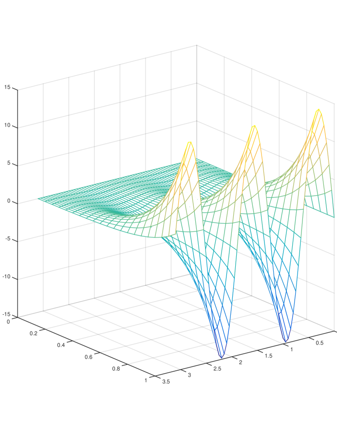
Fig. 1: Carpet plot of exact solution for $n=5$

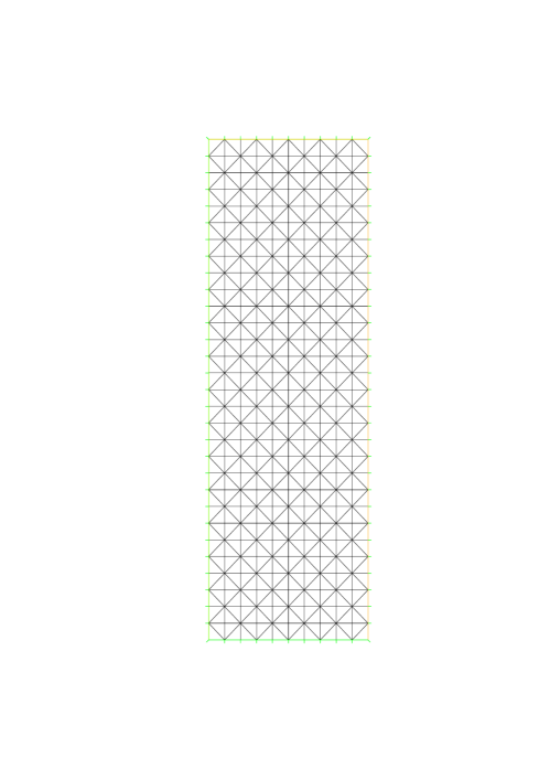
Fig. 2: Example of a computational mesh

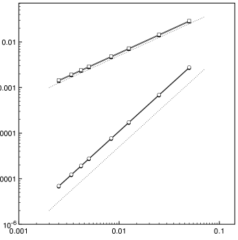
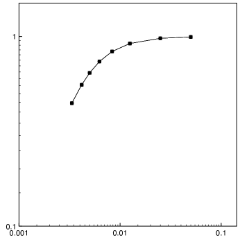
Fig. 3: Relative error against mesh size. $k=1$, from left to right: $n=1$, $n=5$. Square markers indicate $H^{1}$-seminorm errors, circle markers indicate $L^{2}$-errors, filled markers indicate global errors and not filled markers indicate local errors. Dotted reference lines (left plot): top $y=O(h)$, bottom $y=O(h^{2})$

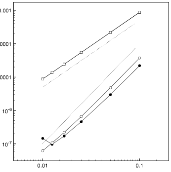
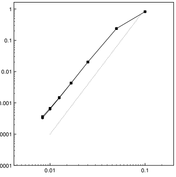
Fig. 4: Relative error against mesh size. $k=2$, from left to right: $n=1$, $n=5$. Square markers indicate $H^{1}$-seminorm errors, circle markers indicate $L^{2}$-errors, filled markers indicate global errors and not filled markers indicate local errors. Dotted reference lines (left plot): top $y=O(h^{2})$, bottom $y=O(h^{3})$, (right plot) $y=O(h^{2})$

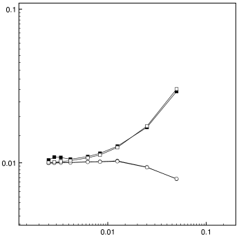
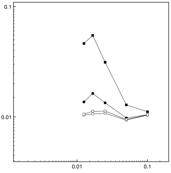
Fig. 5: Relative error against mesh size. Left graphic $k=1$, Neumann data with $2\%$ relative perturbation. Right graphic $k=2$, Neumann data with $2\%$ relative perturbation. Square markers indicate $H^{1}$-seminorm errors, circle markers indicate $L^{2}$-errors, filled markers indicate global errors and not filled markers indicate local errors.

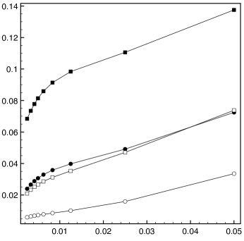
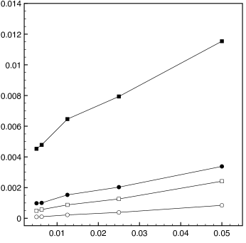
Fig. 6: Relative error against mesh size for case 2. From left to right: $k=1$ and $k=2$. Square markers indicate $H^{1}$-seminorm errors, circle markers indicate $L^{2}$-errors, filled markers indicate global errors and not filled markers indicate local errors.

6 Conclusion

We have derived error estimates for a primal dual mixed finite element method applied to the elliptic Cauchy problem. The results are optimal with respect to the approximation orders of the finite element spaces and the stability of the ill-posed problem. Introducing a special dual stabilizer we reduce the scheme to a least squares mixed method for which the number of degrees of freedom is significantly smaller, the system matrix is symmetric, but the exact local flux conservation is lost. This method satisfies similar estimates, but the results require slightly more regularity of the source term and have slightly worse sensitivity to perturbed data. We then showed that the reduced method can be used in an iterative method to solve the full primal dual formulation, thus recovering local conservation. The estimates show that if the exact solution is smooth the use of high order approximation can pay off. However the amplification of perturbations in data is also stronger with increased approximation order. In numerical experiments we observed that the gain obtained from the high order approximation is more important than the increased sensitivity. Indeed both methods performed better with higher order approximation, in particular for oscillating solutions. As expected from the estimates the accuracy for both methods was similar in our experiments, where the right hand side was zero. The improved local conservation of the full primal dual formulation was observed and the iterative procedure converged to a relative residual of the increment in the $L^{2}$-norm of $O(10^{-6})$ within up to three iterations. Finally we point out the the method presented herein also can be applied to inverse problems subject to the Helmholtz equation, as those discussed in [19].

Appendix

Let $\lambda_{min}(A)$ and $\lambda_{max}(A)$ denote the smallest and largest eigenvalues of the matrix $A$. Assume, without loss of generality, that no $\tilde{F}$ has a corner of the domain through its interior. For a patch $\tilde{F}$ let $\mathcal{N}_{\tilde{F}}$ denote the set of elements with one face entirely in $\tilde{F}$, i.e. not touching the boundary of $\tilde{F}$. Let $\mathcal{N}_{\tilde{P}}$ be the union of the elements $\mathcal{N}_{\tilde{F}}$ and their interior neighbours, that is, any element $K$ such that $K\cap\Sigma=\emptyset$ and $K\cap K^{\prime}\neq\emptyset$ for some $K^{\prime}\in\mathcal{N}_{\tilde{F}}$. We also introduce the set $\mathcal{N}_{\partial\tilde{F}}$ of elements in $\mathcal{N}_{\tilde{F}}$ with a neighbour that intersects $\partial\tilde{F}$. We define the patch $\tilde{P}:=\cup_{K\in\mathcal{N}_{\tilde{P}}}$. Now let $\tilde{\varphi}\in V_{0}^{1}$ such that $\tilde{\varphi}|_{\partial\tilde{P}}=0$ and $\tilde{\varphi}(x_{P})=1$ for any interior vertex $x_{P}$ in $\tilde{P}$. It follows that $\|\nabla\tilde{\varphi}\|_{\tilde{P}}^{2}\lesssim h^{d-2}$. We will first prove, using shape regularity and the properties of $A$, that provided $\mbox{diam}(\tilde{F})/h$ is large enough (but independently of $h$) there exists $c_{0}$, independent of $h$, such that

$$c_{0}h^{-1}\leq\mbox{meas}_{d-1}(\tilde{F})^{-1}\int_{\tilde{F}}A\nabla\tilde{\varphi}\cdot\boldsymbol{\nu}~{}\mbox{d}s=:\Theta(A,\tilde{\varphi}).$$ (6.1)

Here we used that, for any element in $\mathcal{N}_{\tilde{F}}\setminus\mathcal{N}_{\partial\tilde{F}}$, $A\nabla\tilde{\varphi}\cdot\boldsymbol{\nu}\geq\lambda_{min}(A)|\nabla\tilde{\varphi}|$, with $h^{-1}\lesssim|\nabla\tilde{\varphi}|$ on the face intersecting $\tilde{F}$.

$$\int_{\tilde{F}}A\nabla\tilde{\varphi}\cdot\boldsymbol{\nu}~{}\mbox{d}s=\sum_{K\in\mathcal{N}_{\partial\tilde{F}}}\int_{\partial K\cap\tilde{F}}A\nabla\tilde{\varphi}\cdot\boldsymbol{\nu}~{}\mbox{d}s+\sum_{K\in\mathcal{N}_{\tilde{F}}\setminus\mathcal{N}_{\partial\tilde{F}}}\int_{\partial K\cap\tilde{F}}A\nabla\tilde{\varphi}\cdot\boldsymbol{\nu}~{}\mbox{d}s\\ \geq-\sum_{K\in\mathcal{N}_{\partial\tilde{F}}}\lambda_{max}(A)c_{max}h^{-1}h^{d-1}+\sum_{K\in\mathcal{N}_{\tilde{F}}\setminus\mathcal{N}_{\partial\tilde{F}}}\lambda_{min}(A)c_{min}h^{-1}h^{d-1}$$

where $c_{min}$ and $c_{max}$ only depend on the shape regularity of the elements. Observing that $\mbox{card}(\mathcal{N}_{\partial\tilde{F}})=O(h^{2-d})$ and $\mbox{card}(\mathcal{N}_{\mathcal{N}_{\tilde{F}}\setminus\mathcal{N}_{\partial\tilde{F}}})=O(h^{1-d})$ we see that the second sum dominates the first for $\mbox{diam}(\tilde{F})/h$ large enough. This concludes the proof of (6.1).

Define $\varphi_{\tilde{F}}:=\tilde{\varphi}/\Theta(A,\tilde{\varphi})$. By construction

$$\int_{\tilde{F}}A\nabla\varphi_{\tilde{F}}\cdot\boldsymbol{\nu}~{}\mbox{d}s=\mbox{meas}_{d-1}(\tilde{F}).$$

Consider now the $H^{1}$-seminorm of $\varphi_{\tilde{F}}$ on $\tilde{P}$,

$$\|\nabla\varphi_{\tilde{F}}\|_{\tilde{P}}=\|\nabla\tilde{\varphi}\|_{\tilde{P}}/(c_{0}h^{-1})^{2}\lesssim(h^{d-2}/(c_{0}h^{-1})^{2})^{-\frac{1}{2}}\lesssim h^{\frac{d}{2}}.$$ (6.2)

Using a Poincaré inequality we have $\|\varphi_{\tilde{F}}\|_{\tilde{P}}\lesssim h\|\nabla\varphi_{\tilde{F}}\|_{\tilde{P}}$ which together with (6.2) yields the desired bound (3.2).

References

- [1] G. Alessandrini, L. Rondi, E. Rosset, and S. Vessella. The stability for the Cauchy problem for elliptic equations. Inverse Problems, 25(12):123004, 47, 2009.
- [2] M. Azaïez, F. Ben Belgacem, and H. El Fekih. On Cauchy’s problem. II. Completion, regularization and approximation. Inverse Problems, 22(4):1307–1336, 2006.
- [3] F. Ben Belgacem. Why is the Cauchy problem severely ill-posed? Inverse Problems, 23(2):823–836, 2007.
- [4] L. Bourgeois. A mixed formulation of quasi-reversibility to solve the Cauchy problem for Laplace’s equation. Inverse Problems, 21(3):1087–1104, 2005.
- [5] L. Bourgeois. Convergence rates for the quasi-reversibility method to solve the Cauchy problem for Laplace’s equation. Inverse Problems, 22(2):413–430, 2006.
- [6] L. Bourgeois and J. Dardé. About stability and regularization of ill-posed elliptic Cauchy problems: the case of Lipschitz domains. Appl. Anal., 89(11):1745–1768, 2010.
- [7] L. Bourgeois and J. Dardé. A duality-based method of quasi-reversibility to solve the Cauchy problem in the presence of noisy data. Inverse Problems, 26(9):095016, 21, 2010.
- [8] L. Bourgeois and J. Dardé. A quasi-reversibility approach to solve the inverse obstacle problem. Inverse Probl. Imaging, 4(3):351–377, 2010.
- [9] J. H. Bramble, R. D. Lazarov, and J. E. Pasciak. A least-squares approach based on a discrete minus one inner product for first order systems. Math. Comp., 66(219):935–955, 1997.
- [10] S. C. Brenner. Poincaré-Friedrichs inequalities for piecewise functions. SIAM J. Numer. Anal., 41(1):306–324, 2003.
- [11] E. Burman. Stabilized finite element methods for nonsymmetric, noncoercive, and ill-posed problems. Part I: Elliptic equations. SIAM J. Sci. Comput., 35(6):A2752–A2780, 2013.
- [12] E. Burman. Error estimates for stabilized finite element methods applied to ill-posed problems. C. R. Math. Acad. Sci. Paris, 352(7-8):655–659, 2014.
- [13] E. Burman. Stabilized finite element methods for nonsymmetric, noncoercive, and ill-posed problems. Part II: Hyperbolic equations. SIAM J. Sci. Comput., 36(4):A1911–A1936, 2014.
- [14] E. Burman. Stabilised finite element methods for ill-posed problems with conditional stability. Lecture Notes in Computational Science and Engineering, 114:93–127, 2016. cited By 0.
- [15] E. Burman. The elliptic Cauchy problem revisited: control of boundary data in natural norms. C. R. Math. Acad. Sci. Paris, 355(4):479–484, 2017.
- [16] E. Burman. A stabilized nonconforming finite element method for the elliptic Cauchy problem. Math. Comp., 86(303):75–96, 2017.
- [17] E. Burman, P. Hansbo, and M. Larson. Solving ill-posed control problems by stabilized finite element methods: an alternative to Tikhonov regularization. ArXiv e-prints, September 2016.
- [18] E. Burman, J. Ish-Horowicz, and L. Oksanen. Fully discrete finite element data assimilation method for the heat equation. ArXiv e-prints, July 2017.
- [19] E. Burman, M. Nechita, and L. Oksanen. Unique continuation for the Helmholtz equation using stabilized finite element methods. ArXiv e-prints, October 2017.
- [20] E. Burman and L. Oksanen. Data assimilation for the heat equation using stabilized finite element methods. ArXiv e-prints, September 2016.
- [21] P. G. Ciarlet. The finite element method for elliptic problems. North-Holland Publishing Co., Amsterdam-New York-Oxford, 1978. Studies in Mathematics and its Applications, Vol. 4.
- [22] N. Cîndea and A. Münch. Inverse problems for linear hyperbolic equations using mixed formulations. Inverse Problems, 31(7):075001, 38, 2015.
- [23] J. Dardé, A. Hannukainen, and N. Hyvönen. An -based mixed quasi-reversibility method for solving elliptic Cauchy problems. SIAM J. Numer. Anal., 51(4):2123–2148, 2013.
- [24] A. Ern and J.-L. Guermond. Theory and practice of finite elements, volume 159 of Applied Mathematical Sciences. Springer-Verlag, New York, 2004.
- [25] R. S. Falk. Approximation of inverse problems. In Inverse problems in partial differential equations (Arcata, CA, 1989), pages 7–16. SIAM, Philadelphia, PA, 1990.
- [26] R. S. Falk and P. B. Monk. Logarithmic convexity for discrete harmonic functions and the approximation of the Cauchy problem for Poisson’s equation. Math. Comp., 47(175):135–149, 1986.
- [27] A. Fumagalli and E. Keilegavlen. Dual Virtual Element Methods for Discrete Fracture Matrix Models. ArXiv e-prints, November 2017.
- [28] J. Hadamard. Sur les problèmes aux derivées partielles et leur signification physique. Bull. Univ. Princeton, 1902.
- [29] H. Han. The finite element method in the family of improperly posed problems. Math. Comp., 38(157):55–65, 1982.
- [30] F. Hecht. New development in freefem++. J. Numer. Math., 20(3-4):251–265, 2012.
- [31] R. Lattès and J.-L. Lions. The method of quasi-reversibility. Applications to partial differential equations. Translated from the French edition and edited by Richard Bellman. Modern Analytic and Computational Methods in Science and Mathematics, No. 18. American Elsevier Publishing Co., Inc., New York, 1969.
- [32] Y. Liu, J. Wang, and Q. Zou. A Conservative Flux Optimization Finite Element Method for Convection-Diffusion Equations. ArXiv e-prints, October 2017.
- [33] P. Monk and E. Süli. The adaptive computation of far-field patterns by a posteriori error estimation of linear functionals. SIAM J. Numer. Anal., 36(1):251–274, 1999.
- [34] L. E. Payne. Bounds in the Cauchy problem for the Laplace equation. Arch. Rational Mech. Anal., 5:35–45 (1960), 1960.
- [35] L. E. Payne. On a priori bounds in the Cauchy problem for elliptic equations. SIAM J. Math. Anal., 1:82–89, 1970.
- [36] H.-J. Reinhardt, H. Han, and Dinh Nho Hào. Stability and regularization of a discrete approximation to the Cauchy problem for Laplace’s equation. SIAM J. Numer. Anal., 36(3):890–905, 1999.
- [37] A. N. Tikhonov and V. Y. Arsenin. Solutions of ill-posed problems. V. H. Winston & Sons, Washington, D.C.: John Wiley & Sons, New York-Toronto, Ont.-London, 1977. Translated from the Russian, Preface by translation editor Fritz John, Scripta Series in Mathematics.
- [38] C. Wang and J. Wang. A Primal-Dual Weak Galerkin Finite Element Method for Second Order Elliptic Equations in Non-Divergence Form. ArXiv e-prints, October 2015.
- [39] C. Wang and J. Wang. A Primal-Dual Weak Galerkin Finite Element Method for Fokker-Planck Type Equations. ArXiv e-prints, April 2017.