X-ray Light Curve and Spectra of Shock Breakout in a Wind

Abstract

We investigate the properties of X-ray emission from shock breakout of a supernova in a stellar wind. We consider a simple model describing aspherical explosions, in which the shock front with an ellipsoidal shape propagates into the dense circumstellar matter. For this model, both X-ray light curves and spectra are simultaneously calculated using a Monte Carlo method. We show that the shock breakout occurs simultaneously in all directions in a steady and spherically symmetric wind. As a result, even for the aspherical explosion, the rise and decay timescales of the light curve do not significantly depend on the viewing angles. This fact suggests that the light curve of the shock breakout may be used as a probe of the wind mass loss rate. We compare our results with the observed spectrum and light curve of XRO 080109/SN 2008D. The observation can be reproduced by an explosion with a shock velocity of 60% of the speed of light and a circumstellar matter with a mass loss rate of $5\times 10^{-4}M_{\odot}$ yr^-1.

1. Introduction

A core-collapse supernova emits a bright ultraviolet (UV)/X-ray flash, so-called ”shock breakout”, when photons generated from the shock escape upstream. Shock breakout has been studied for several decades since Klein & Chevalier (1978) and Falk (1978). The timescale of the emission is determined by the light crossing time of the radius of the source and the diffusion timescale of photons in the unshocked or shocked matter (e.g. Ensman & Burrows, 1992; Matzner & McKee, 1999). Shock breakout is a powerful probe of the stellar radius and the structure of the outer layer of the star, since it should be associated with all core-collapse supernovae, and the emission properties are highly sensitive to the behavior of the shock.

In 2008, the Swift/XRT accidentally detected X-ray outburst (XRO) 080109 (Soderberg et al., 2008), which was associated with a type Ib supernova (SN) 2008D (Mazzali et al., 2008; Malesani et al., 2009; Modjaz et al., 2009; Tanaka et al., 2009b). The luminosity rapidly reached the maximum in the first $\sim 100$ sec and exponentially decayed until 600 sec from the onset of the outburst. The peak luminosity and total radiated energy are $6\times 10^{43}$ erg s^-1 and $2\times 10^{46}$ erg, respectively. The Swift/XRT spectrum is well fitted by a power-law function, rather than a Planck function. Soderberg et al. (2008) also reported that a $UV/opt$ emission was detected by the Swift/UVOT $\sim 1$ day after XRO 080109, and a decreasing X-ray emission [$L=(1.0\pm 3.0)\times 10^{39}$ erg s^-1 in the energy range of 0.3–10 keV] by the Chandra X-ray Observatory $\sim 10$ days after the Swift discovery. XRO 080109 and the subsequent fainter X-ray emission is believed to originate from shock breakout and interaction of the shock with a circum-stellar matter (CSM) (Soderberg et al., 2008; Chevalier & Fransson, 2008).

The timescale of XRO 080109 is closely related to the shock radius at the moment of breakout. When interpreting the rise time as the light crossing time of the breakout radius, it must be $\approx 10^{12}$ cm (Soderberg et al., 2008). Since it is larger than the typical radius of a Wolf-Rayet star, XRO 080109 is believed to originate from a dense CSM. The observed duration is consistent with the diffusion timescale of photons in the unshocked CSM, in which the shock breaks out at the radius of 1.1–1.6$\times 10^{12}$ cm (Balberg & Loeb, 2011). If the rise time is regarded as the shock expansion timescale, the shock radius is estimated to be $\approx 6\times 10^{11}$ cm (Svirski & Nakar, 2014). Though the two estimated values are different by a factor of a few, they agree upon the excess of the breakout radius compared to the typical radius of a Wolf-Rayet progenitor. In general, Wolf-Rayet stars blow winds with terminal velocities $v_{\rm t}$ of $v_{\rm t}\sim$1,000 km s^-1 (Prinja et al., 1990; Hamann et al., 1995) at rates $\dot{M}$ in the range of $10^{-5}$ to $10^{-4}M_{\odot}$ yr^-1 (Hamann et al., 1995; Nugis et al., 1998). Since a wind mass loss event is known to play a significant role in the evolution of a massive star (Maeder & Meynet, 1987; Meynet et al., 1994), studying shock breakout also enriches the understanding of massive star evolution shortly before the explosion. For this importance, the properties (such as timescale and luminosity evolution) of emission from the shock breakout in a wind have been predicted by several theoretical studies (e.g. Balberg & Loeb, 2011; Moriya et al., 2011; Chevalier & Irwin, 2011, 2012; Svirski et al., 2012; Svirski & Nakar, 2014).

The origin of the observed spectrum of XRO 080109 has been argued in several articles. The observed spectrum can also be fitted by a combination of two blackbody components, but the photospheric radii are far smaller than the typical radius of a Wolf-Rayet star (Li, 2008). Soderberg et al. (2008) attributes the power-law spectral feature to electron (”bulk-Comptonization”) scattering across a shock. In fact, Suzuki & Shigeyama (2010a) numerically examined how the photon energies increase due to this effect. Their results imply that the observed power-law X-ray spectrum requires a shock velocity higher than $0.3c$, where $c$ denotes the speed of light. The effect of bulk-Comptonization has also been studied by Wang et al. (2007), in which mildly relativistic shock breakout in a dense CSM is applied for the low-luminosity GRB 060218/SN 2006j (Campana et al., 2006). Similar studies have been performed for shocks with lower velocities ($\lesssim 10^{4}$ km s^-1) by Svirski et al. (2012) and Chevalier & Irwin (2012), applied to the luminous Type IIn SN 2006gy. The scattering process decreases photon energies in this particular supernova.

In addition to the presence of the CSM and the bulk-Comptonization, the asphericity of the shock front might also be important to determine the emission properties of shock breakout. Suzuki & Shigeyama (2010b) suggested that the shape of the light curve can reflect the degree of shock asphericity and the viewing angle. Couch et al. (2011) investigated the influence of shock asphericity on the light curve and spectrum by using results of their two-dimensional hydrodynamical simulations of a jet-driven supernova. However, they do not take the influence of bulk-Compton scattering into the calculation of the spectrum. Suzuki et al. (2016) recently performed 2D radiation hydrodynamic simulations for a blue supergiant exploding in a steady wind. Since bipolar explosions result in the shock appearing sequentially, the light curve would have a broader peak compared to the case of a spherical shock.

Despite a large number of studies having investigated the emission properties in detail, there have been no studies that reproduce both the observed X-ray spectrum and light curve by taking bulk-Comptonization into account. In this paper, we aim to investigate the influence of shock asphericity and bulk-Comptonization on the properties of emission from shock breakout in a wind. For this purpose, we perform radiative transfer calculations using a Monte-Carlo method. In Section 2, we describe the settings for the shock and Monte-Carlo calculation. In Section 3, we show the results and comparisons with the observed properties of XRO 080109/SN 2008D. In Section 4, we conclude this paper.

2. Methods

We calculate X-ray light curves and spectra of shock breakout emission in a dense CSM. In the following subsections, we describe our model for the propagation of the shock (§2.1) and the method to calculate radiative transfer (§2.2).

2.1. Model for shock

To capture the properties of X-ray emission, we adopt a simple model of shock breakout in a wind as described below (Figure 1). Our calculation does not take into account the feedback from emission to the fluid motion.

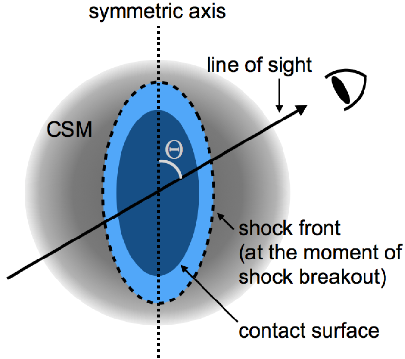
Figure 1.— Schematic view of an ellipsoidal shock propagating into a steady, spherically symmetric CSM. The degree of the shock asphericity is characterized by the oblateness $f$. The position of the shock front corresponds to the dashed curve at the moment of breakout.

The matter is radiation dominated (the adiabatic index $\gamma$ equals to 4/3), and the radiation and matter are in thermal equilibrium below the photosphere. Here we focus on inverse Compton scattering in the shocked CSM of interest. For that, we think of supernova ejecta as a piston, and focus on modeling the forward shock propagating in the CSM. We ignore the presence of the shocked ejecta. Since the supposed ejecta density, $\approx 10^{20}$ cm^-3 at the moment of breakout (hereafter $t=t_{\rm b}$ where $t$ denotes the time measured from the moment of explosion) is orders of magnitude higher than that of the shocked CSM ($\approx 10^{13}$ cm^-3), photons would be absorbed or scattered immediately at the contact surface. (Inward traveling photons generated from the shock front can be blocked by a shell filled by ejecta with a uniform density and a mass of $\Delta M_{\rm ej}\sim 2\times 10^{-7}M_{\odot}$, the same order of magnitude as the total mass of the shocked CSM, $M_{\rm sh}=1\times 10^{-7}M_{\odot}$, at $t=t_{\rm b}$. Here $\Delta M_{\rm ej}$ is estimated from the shell width $R_{\rm c}-r_{\rm min}$ of $1/\kappa\rho_{\rm ej}=3\times 10^{4}$ cm, where $\kappa$=0.2 cm² g^-1 is the opacity for electron scattering, $R_{\rm c}$ the radius of the contact surface, and $\rho_{\rm ej}=1.8\times 10^{-4}$ g cm^-3 the mass density of ejecta). To see the influence of the structure behind the shock on the emission properties (shapes of the light curve and spectrum), we compare results of calculations with that using self-similar solutions of Chevalier (1982) with different density structures of the ejecta. As shown in Figure 13 (Appendix B), there is no significant difference in the shapes of the X-ray light curves between the models. We obtain spectra with similar shapes as long as the density of the ejecta has a steep slope ($n\geq 10$) as a function of radius (see Figure 14). Thus three different regions (unshocked CSM, shocked CSM, and unshocked ejecta) are under consideration. Both the shocked CSM and ejecta move at constant velocities. The ejecta are assumed to have a uniform density and evolve in homologous expansion. The total mass is $10M_{\odot}$.

We consider a shock having an ellipsoidal shape. The shock radial velocity follows the formula

$$v(f,\theta)=\dfrac{1-f}{[(1-f)^{2}\cos^{2}\theta+\sin^{2}\theta]^{1/2}}\times v(f,0),$$ (1)

where $f$ denotes the oblateness of the shock front, $\theta$ the angle measured from the symmetric axis. If the kinetic energy of the ejecta is fixed, the shock velocity at $\theta=0$ can be written as follows (Appendix A).

$$v(f,0)=\sqrt{3}\times v_{f=0}\times(2f^{2}-4f+3)^{-1/2},$$ (2)

where $v_{f=0}$ is the shock velocity in the spherically symmetric case. In this study, $v_{f=0}=0.6c$. Figure 2 shows the angular dependence of $v$ for $f=0$ (spherical), 0.1, 0.3, and 0.5.

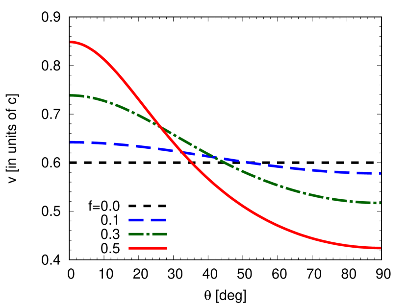
Figure 2.— Angular dependence of the shock velocity $v$.

The wind is supposed to be stationary, spherically symmetric, and emanate from a carbon-oxygen layer. The electron number density $n_{1}$ of the unshocked CSM follows the equation

$$n_{1}=\dfrac{A}{r^{2}},$$ (3)

where $r$ is the radius measured from the center of the progenitor, and $A$ a constant. The optical depth $\tau$ of the unshocked CSM must be equal to $c/v$ when the shock propagating at a speed $v$ breaks out. The characteristic timescale of the emission must strongly depend on $R_{\rm b}$. We can determine the shock radius at the moment of breakout $R_{\rm b}$ for $f=0$ by a condition that the rise time of the observed emission is equal to the light crossing time $R_{\rm b}/c$. If we adopt $\Delta t_{\rm rise}\approx 100$ sec, then $R_{\rm b}$ becomes $3\times 10^{12}$ cm. Therefore the constant $A$ can be uniquely determined by the following equation,

$$A=\frac{c}{v_{f=0}}\left[\sigma_{\rm kl}\int^{\infty}_{R_{\rm b}}r^{-2}dr\right]^{-1},$$ (4)

with a free parameter $v_{f=0}$. $\sigma_{\rm kl}$ is the Klein-Nishina cross section for a photon with an energy corresponding to the peak energy of a blackbody radiation. From the assumption of $v_{f=0}=0.6c$, $A=7.5\times 10^{36}$ cm^-1. When $f\neq 0$, $R_{\rm b}$ has an angular dependence as written by

$$R_{\rm b}=A\sigma_{\rm kl}\times\dfrac{v(f,\theta)}{c}.$$ (5)

This equation indicates that the shock breaks out at the same moment $R_{\rm b}/v$ in all directions (independent of $\theta$) if it has constant velocities. If the radial velocity of the unshocked CSM is 1,000 km s^-1, the mass loss rate $\dot{M}$ becomes $5\times 10^{-4}$ $M_{\odot}$ yr^-1. The rate is one order of magnitude higher than that for an ordinary Wolf-Rayet star, but still consistent with that of a luminous blue variable (Humphreys & Davidson, 1994).

We can estimate the thickness $\Delta R$ of the shocked CSM assuming a uniform density $n_{2}$ there. The number density $n_{2}$ of the shocked CSM at the shock front satisfies the Rankine-Hugoniot relation

$$\dfrac{n_{2}}{n_{1}}=\dfrac{\gamma+1}{\gamma-1}.$$ (6)

A relation between the masses of the matter swept by the shock and the shocked CSM is written by

$$4\pi R^{2}\rho_{2}\Delta R=4\pi AR,$$ (7)

where $R=v(f,\theta)t$ is the shock radius. From equations (6) and (7), $\Delta R$ equals to $(\gamma-1)/(\gamma+1)\times R=R/7$. Therefore the density $\rho_{2}=2.0\times 10^{-11}$ g cm^-3 and the pressure $p_{2}=6.3\times 10^{9}$ g cm^-1 s^-2 at the moment of shock breakout ($R=R_{\rm b}$). Under the assumption of radiation-dominated state and local thermodynamic equilibrium, the temperature for the shocked CSM is determined by $T_{2}=(3p_{2}/a)^{1/4}=1.3\times 10^{6}$ K and that for the ejecta by $T_{\rm ej}=(3\rho_{\rm ej}v^{2}_{f=0}/a)^{1/4}=6.9\times 10^{7}$ K, where $a$ is the radiation constant. The temperature of the unshocked CSM is $T_{1}=1.0\times 10^{4}$ K, which is close to the typical effective temperature of a Wolf-Rayet star (Herald et al., 2000). The shocked CSM and the ejecta are assumed to have the same velocities $v(f,\theta)$. The assumption of $10M_{\odot}$ ejecta with high velocities of $v(f,\theta)$ itself is of cause too energetic. Again, we note that photons do not enter a deep layer of the ejecta, so that only a very low-mass ($\sim 2\times 10^{-7}M_{\odot}$) of ejecta is required to have high velocities as $v(f,\theta)$. The kinetic energy of the ejecta in this region is $1\times 10^{47}$ erg. For that reason, the supposed situation is not so bad in the region calculated in this work.

2.2. Monte-Carlo method

Using the settings of Section 2.1, we calculate radiative transfer of thermal photons by using a Monte-Carlo method. The basic construction of the code is the same one as we used in our previous study (Ohtani et al., 2013). Here we describe several assumptions made in this study.

Photons are isotropically generated at the shock front over a period of $\Delta t_{\rm ph}$=0.5 sec. The period is determined so that the total radiation energy roughly equals to the total emitted energy estimated from the Swift/XRT observation. 1,000 seed photons are generated every $5\times 10^{-4}$ sec with an energy distribution following the Planck distribution in the rest frame of the fluid. If $f=0$, the photospheric temperature is 0.11 keV (hereafter $k_{\rm B}T_{f=0}$; $T_{f=0}=T_{2}$) at the moment of breakout, and the total energy $E_{\rm tot,i}$ radiated in the time interval $\Delta t_{\rm ph}$ is $\sim 6\times 10^{45}$ erg. After the shock breakout, some photons diffuse out of the shock front and reduce the pressure $p_{2}$ in the shocked CSM but not significantly change the temperature, which is proportional to $p^{1/4}_{2}$. (From the thermal energy of the shocked CSM, $4\pi R^{2}\Delta RaT^{4}_{2}=1\times 10^{48}$ erg, the change in the temperature $T_{2}$ is estimated to be $\sim 0.2$%.) Thus we do not take into account this effect in the radiative transfer calculations.

We should note that the energy $E_{\rm tot,i}$ released by radiation is 1–2 orders of magnitude lower than the kinetic energy of the shocked matter, which must be comparable to the thermal radiation in an ordinary shock. We consider that this is because a major portion of photons generated in the ejecta remains trapped. To discuss that, a comparison of the dynamical timescale (hereafter $t_{\rm dyn}$) of the shock, $R_{\rm b}/0.6c\sim 170$ sec, with the diffusion time of photons in the ejecta is needed. We have estimated the diffusion time $t_{\rm diff}$ in a region between $r=r_{\rm min}$ and $r=R$. If the flow expands linearly with time, the optical depth of the above region becomes unity when the shock reaches a radius (hereafter $R^{\prime\prime}_{\tau=1}$) of $\sim 7\times 10^{12}$ cm. Thus the diffusion time $t_{\rm diff}$ becomes $(7-3)\times 10^{12}\text{ cm}/v\sim 200$ sec. Since $t_{\rm diff}$ is longer than $t_{\rm dyn}$, it seems that a major portion of photons is still trapped in the ejecta.

The generated photons are assumed to interact with matter via inverse-Compton scattering and free-free absorption. In the shocked CSM, the effective optical thickness $\tau_{\star}$ can be estimated by

$$\tau_{\star}=\sqrt{\alpha^{\rm ff}(\alpha^{\rm ff}+n_{2}\sigma_{\rm kl})}\Delta R$$ (8)

where $\alpha^{\rm ff}$ is the absorption coefficient, due to free-free transition of electrons

$$\alpha^{\rm ff}=3.7\times 10^{8}T^{-1/2}Z^{2}n_{1}n_{\rm i}\nu^{-3}(1-e^{-h\nu/k_{\rm B}T})\bar{g}_{\rm ff}\text{ cm}^{-1}$$ (9)

(Rybicki & Lightman, 1979). $T$ is the temperature, $Z$ the atomic number, $n_{\rm i}$ the number density of ion, $h$ the Planck constant, $\nu$ the frequency, and $\bar{g}_{\rm ff}(\sim 1)$ the gaunt factor. If $f=0$, $\tau_{\star}=4\times 10^{-4}\ll 1$ for $h\nu=$0.3 keV and $Z=8$ at the moment of shock breakout. Therefore most photons are not absorbed by electrons.

The process of photon-electron coupling is discussed by Nakar & Sari (2010) and Katz et al. (2010) for shock breakout at a stellar surface, and by Svirski et al. (2012) for that in a wind. Here we estimate the total number of thermal photons produced by bremsstrahlung emission. The total emissivity integrated over frequency is expressed by

$$\varepsilon^{\rm ff}=1.4\times 10^{-27}T^{1/2}n_{\rm el}n_{\rm i}Z^{2}\bar{g}_{\rm B},$$ (10)

where $n_{\rm el}$ is the electron number density, $n_{\rm i}$ the ion number density, $Z$ the electric charge of the ion, and $\bar{g}_{\rm B}\sim 1$ the gaunt factor (Rybicki & Lightman, 1979). Assuming $n_{\rm el}=n_{\rm ej}$ ($n_{\rm ej}=6\times 10^{19}$ cm^-3: electron number density in the ejecta), $T=T_{\rm ej}$ and fully ionized oxygen gas, Equation (10) yields $\varepsilon^{\rm ff}=3\times 10^{17}$ erg s^-1 cm^-3. Therefore the energy $E^{\rm ff}_{\nu}$ radiated from the ejecta per unit time is roughly evaluated by $4\pi R_{\rm b}^{2}(1/\kappa\rho_{\rm ej})\varepsilon^{\rm ff}=1\times 10^{48}$ erg s^-1, and the time required to release the energy of $E_{\rm tot,i}$ is $6\times 10^{-3}$ sec. (Dividing $E^{\rm ff}$ by $3k_{\rm B}T_{f=0}$, we can roughly estimate the number of photons as $2\times 10^{57}$ s^-1.) Since the required time is shorter than $\Delta t_{\rm ph}$, we can consider that the generated photons are abundant enough so that the radiation and matter achieve thermal equilibrium.

Under the assumption of fully-ionized gas, possible bound-free absorption is neglected. In order to show the validity of this assumption, we estimate the timescale for photoionization of oxygen in a process similar to that of Suzuki & Shigeyama (2010a). The bound-free cross section of O VI ions is written by

$$\sigma_{\rm bf}=\left(\dfrac{64\pi ng_{\rm bf}}{3\sqrt{3}Z^{2}}\right)\alpha_{\rm fs}a^{2}_{B}\left(\dfrac{\chi}{h\nu}\right)^{3}$$ (11)

where $n=1$ denotes the principal quantum number, $g_{\rm bf}\sim 1$ the bound-free gaunt factor, $\alpha_{\rm fs}$ the fine structure constant, $a_{B}$ the Bohr radius, and $\chi=Z^{2}\alpha^{2}_{\rm fs}m_{\rm el}c^{2}/(2n^{2})=0.87$ keV ($m_{\rm el}$: electron mass) the ionization potential (Rybicki & Lightman, 1979). For photons with energy $3k_{\rm B}T_{f=0}$, Equation (11) yields $\sigma_{\rm bf}=2\times 10^{-18}$ cm${}^{2}\gg\sigma_{\rm kl}$. Though the fact indicates that bound-free absorption is a dominant source of opacity, the interaction would not significantly affect the non-thermal component of the X-ray spectrum due to a short timescale of photoionization. The timescale can be estimated by the total emitted energy and number of non-thermal X-ray photons. Using the luminosity of the thermal emission expressed by

$$L_{\rm th}=4\pi R^{2}_{\rm b}\sigma_{\rm SB}T^{4}_{f=0}=2\times 10^{46}\text{ erg s}^{-1},$$ (12)

($\sigma_{\rm SB}=ac/4$: the Stefan-Boltzmann constant) and the time interval $\Delta t_{\rm ph}$, the total energy becomes

$$E_{\rm th}=L_{\rm th}\dfrac{c\Delta t_{\rm ph}}{v_{f=0}}=2\times 10^{46}\text{ erg}.$$ (13)

Thus the number density of photons with energies of few keV is

$$n_{\rm ph}=\dfrac{\epsilon E_{\rm th}/\text{few keV}}{4\pi R^{2}_{\rm b}c\Delta t_{\rm ph}}\approx 10^{18}\epsilon\text{ cm}^{-3},$$ (14)

where $\epsilon E_{\rm th}$ (here $\epsilon$ is supposed to be $\sim 0.1$) is the total energy of non-thermal photons. Therefore, the timescale for bound-free absorption is

$$\tau_{\rm bf}=\dfrac{1}{c\sigma_{\rm bf}n_{\rm ph}}\approx 10^{-9}\text{ s}$$ (15)

Then we estimate the timescale of radiative recombination for fully ionized oxygen written by

$$\tau_{\rm rad}=\dfrac{1}{\alpha^{\rm rad}_{Z}\bar{n}_{2}},$$ (16)

where

$$\alpha^{\rm ff}_{Z}=5.197\times 10^{-14}Z\beta^{-1/2}(0.4288+0.5\ln\beta+0.469\beta^{-1/3})\text{ cm}^{3}\text{ s}^{-1},$$ (17)

where $\beta=\chi/(k_{\rm B}T)$ (Seaton, 1959). Substituting $T=T_{f=0}$ into the equations above, $\tau_{\rm rad}$ becomes 0.6 sec, which is far longer than $\tau_{\rm bf}$.

We can expect from a comparison of the estimated $\tau_{\rm rad}$ and $\tau_{\rm bf}$ that most elements become fully ionized immediately so that photons with energies of few keVs would not be influenced by bound-free absorption in the shocked CSM. In the unshocked CSM, we obtain $\tau_{\rm bf}\approx 10^{-7}$ sec and $\tau_{\rm rad}=0.4$ sec, by replacing $\Delta t_{\rm ph}$ by the diffusion timescale of photons $\sim 100$ sec (calculated in Section 3.1) in Equation (14), $T$ by $T_{1}$ and $\bar{n}_{2}$ by $n_{1}$ at the shock front in Equations (16) and (17). The small $\tau_{\rm bf}/\tau_{\rm rad}$ ratio allows neglecting the influence of bound-free transition.

Once a photon reaches the surface with an optical depth $\tau$ of $10^{-2}$, it is supposed to escape from the CSM. The calculation stops when the shock front reaches the surface of $\tau=10^{-2}$.

3. Results

First of all, we calculate the X-ray light curve and spectrum for a spherically symmetric supernova ($f=0$), and compare them with the observation of XRO 080109. Then we show the dependence on the oblateness $f$ of the shock and the viewing angle $\Theta$.

3.1. Spherically symmetric shock

Figure 3 shows the light curve in the energy range from 0.3 keV to 10 keV covered by the Swift/XRT. The luminosity rapidly increases for the first 40 sec, and exponentially decreases for the subsequent several hundred seconds, as $L\propto\exp[(t_{\rm obs}-t_{\rm peak})/t_{e}]$ where $t_{\rm peak}=40$ sec and $t_{\rm e}=200$ sec. The time interval between the onset and the peak (hereafter $\Delta t_{\rm rise}$) depends primarily on the light crossing time $\Delta t_{\rm lc}$ of the size of the emerging shock, and secondarily on the diffusion timescale of photons in the shocked CSM. We should note that there is a weak but not negligible influence of relativistic effects on the motion of photons. A photon does not travel toward the observer if the angle between the line of sight and the radial direction exceeds $\tan^{-1}(c\gamma^{-1}v^{-1})\sim 50$ deg. Hereafter the threshold angle is referred to as $\theta_{\rm rel}$. Therefore $\Delta t_{\rm lc}=R_{\rm b}(1-\cos\theta_{\rm rel})/c=30$ sec. The diffusion time $t^{\prime}_{\rm diff}$ of photons in the shocked CSM is determined by the radius $R_{\tau=1}$ at which the optical depth of the shocked CSM becomes unity. From the definition of the CSM density, Equations (3) and (4), $R_{\tau=1}\sim 5\times 10^{12}$ cm. The length of $t^{\prime}_{\rm diff}$ depends on the optical depth between $r=R_{\rm b}$ and $R_{\tau=1}$. It would equal to $(R_{\rm b}-R_{\tau=1})/v=110$ sec.

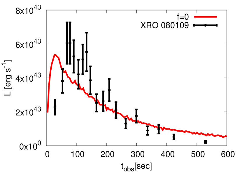
Figure 3.— Light curve (0.3–10 keV) of emission originating from a spherically symmetric shock. The superposed bars are the observed data of XRO 080109. The time is measured from the moment when the first photon passes a large spherical surface concentric with the ejecta.

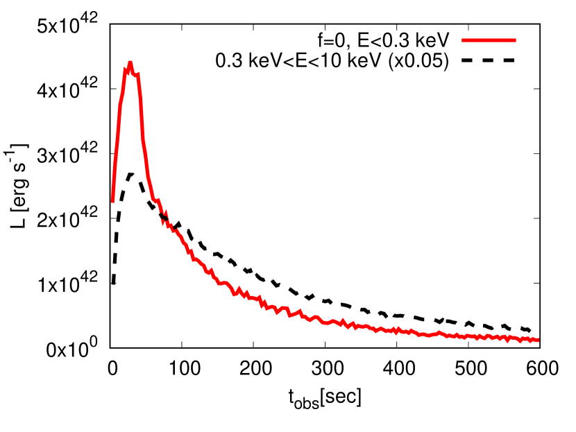
Figure 4.— Comparison of the light curves in the energy range of 0.3-10 keV (black dashed line) and below 0.3 keV (red solid line).

The decay time is related to the light crossing time of the radius $R_{\rm final}$ at which photons are scattered for the last time, and the photon diffusion time in the unshocked CSM. For example, if a photon last scatters off an electron at a radius of $\sim 10R_{\rm b}$, the light crossing time equals to $\sim 10R_{\rm b}/c=1000$ sec. We can expect that nearly $\sim 10$% of generated photons can scatter off electrons between this radius and infinity because the optical depth $\tau$ of the outside matter is not far smaller than 0.1, implying that the scattering probability is close to $1-\exp(-\tau)\sim 0.1$. Therefore the emission can last for several hundreds of seconds. The time constant $t_{\rm e}$ (measured from $t=t_{\rm peak}$) is also related to the optical depth of the unshocked CSM. Because the probability that photons travel straight in the unshocked CSM is $\exp(-\tau)$ and $t_{\rm obs}-t_{\rm peak}$ is inverse proportional to $\tau$, $t_{\rm e}$ corresponds to the time when the luminosity becomes $L_{\rm peak}e^{-1}$. The photon diffusion time is $(R_{\rm b}-R_{\tau=1})/v=110$ sec in the unshocked CSM. The period $\Delta t_{\rm ph}$ over which the shock front emits photons does not influence on the shape of the light curve as long as it is much shorter than the duration.

The overall shape of the light curve consisting of the rapid rise and the exponential decay resembles that of the observed emission in the energy range of the Swift/XRT. Though the length of $\Delta t_{\rm rise}$ is 40 sec in the calculation, which is shorter than the observation, it would be improved when considering a higher density CSM, in which the breakout radius $R_{\rm b}$ becomes $\sim 6\times 10^{12}$ cm. Note that the maximum luminosity should not be discussed in this study, because it is proportional to the assumed period of photon generation and thus can be easily adjusted without additional simulations. Figure 4 shows the light curve for the energy lower than 0.3 keV. Due to absorption, the luminosity decreases rapidly compared to that for 0.3–10 keV, so that the e-folding time $t_{\rm e}$ is as short as 120 sec. There is no significant difference between the rise times for energy lower than 0.3 keV and for 0.3–10 keV.

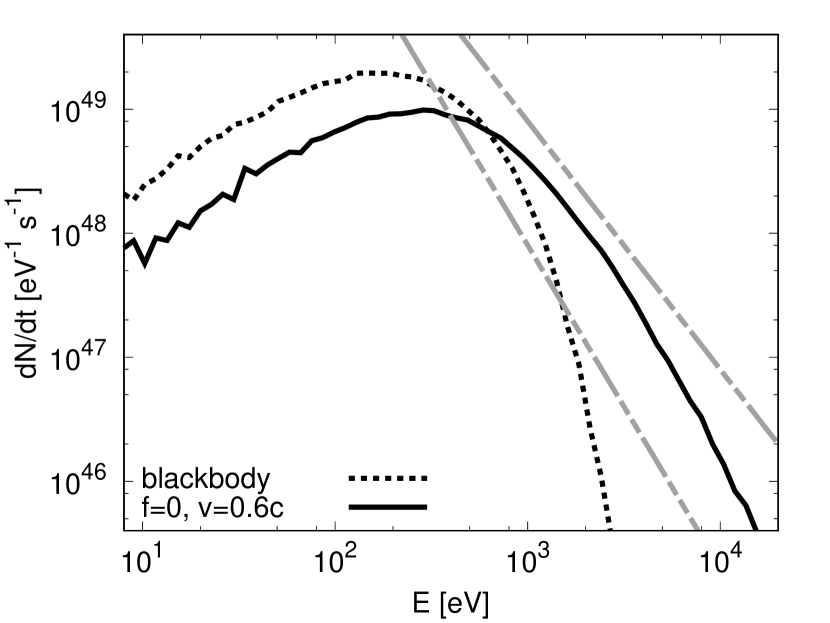
Figure 5.— Time-integrated spectrum of emission from a spherically symmetric shock (solid curve). The dotted curve represents a blackbody spectrum at a temperature of $k_{\rm B}T_{\rm b}$. The gradients of the straight lines are -2.0 and -2.6, which correspond to the $\pm 1\sigma$ values of those of the observed Swift/XRT spectrum.

Figure 5 shows the time-integrated spectrum. The dotted line displays the blackbody with a temperature of $k_{\rm B}T_{f=0}$. Photons following zigzag paths across the shock front receive the kinetic energies of electrons. Their maximum energies reach $E\sim m_{\rm el}v^{2}\sim 10$ keV. The high-energy tail (1–7 keV) of the spectrum can be fitted by a power-law distribution, and the gradient lies in the $1\sigma$ error range of the observed X-ray spectrum (shown by the straight lines in Figure 5).

Comparisons of our results with the observations of XRO 080109 show that the shape of the observed X-ray light curve and the spectrum can be reproduced by the emission generated from a spherically symmetric shock with a velocity of $0.6c$ and a wind with a mass loss rate of $5\times 10^{-4}M_{\odot}$ yr^-1. Here the total radiation energy $E_{\rm tot,f}$ is $2\times 10^{46}$ erg, about 3 times higher than that before electron scattering ($E_{\rm tot,i}$). The total kinetic energy $E_{\rm sh}$ of the shocked CSM is $4\pi R^{2}_{\rm b}\rho_{2}\Delta Rv^{2}=2\times 10^{47}$ erg at the moment of shock breakout. From the relatively small ratio of $E_{\rm tot,f}-E_{\rm tot,i}$ to $E_{\rm sh}$, we can expect that radiation feedback would not induce a significant change of electron temperature.

3.2. Aspherical shock

We investigate the influence of the asphericity of the shock on the light curve and the spectrum. Previous calculations (Suzuki & Shigeyama, 2010b; Couch et al., 2011; Matzner et al., 2013; Salbi et al., 2014; Suzuki et al., 2016) investigated aspherical shock breakout in the vicinities of the stellar surfaces without thick CSM. Caused by the significant time lags between the shocks breaking of their tops and sides, the calculated light curves show the broader peaks compared to that for a spherical shock. Situation of our calculation is fairly different from that, as the shock breakout occurs simultaneously in all directions due to the assumptions of the thick, steady, and spherically symmetric wind and a constant shock velocity $v(f,\theta)$. We should note that in reality, non-radial motions of ejecta play important roles along the stellar surface. If the asphericity (or ”obliquity”) in the ejecta motion is limited to a thin outer layer of the star and the effect of radiation is neglected, non-radial flows are believed to suppress the shock (Matzner et al., 2013). Thus the assumptions in our model need somewhat energetic explosion process, such as a jet-like explosion or a prolonged activity of the central engine.

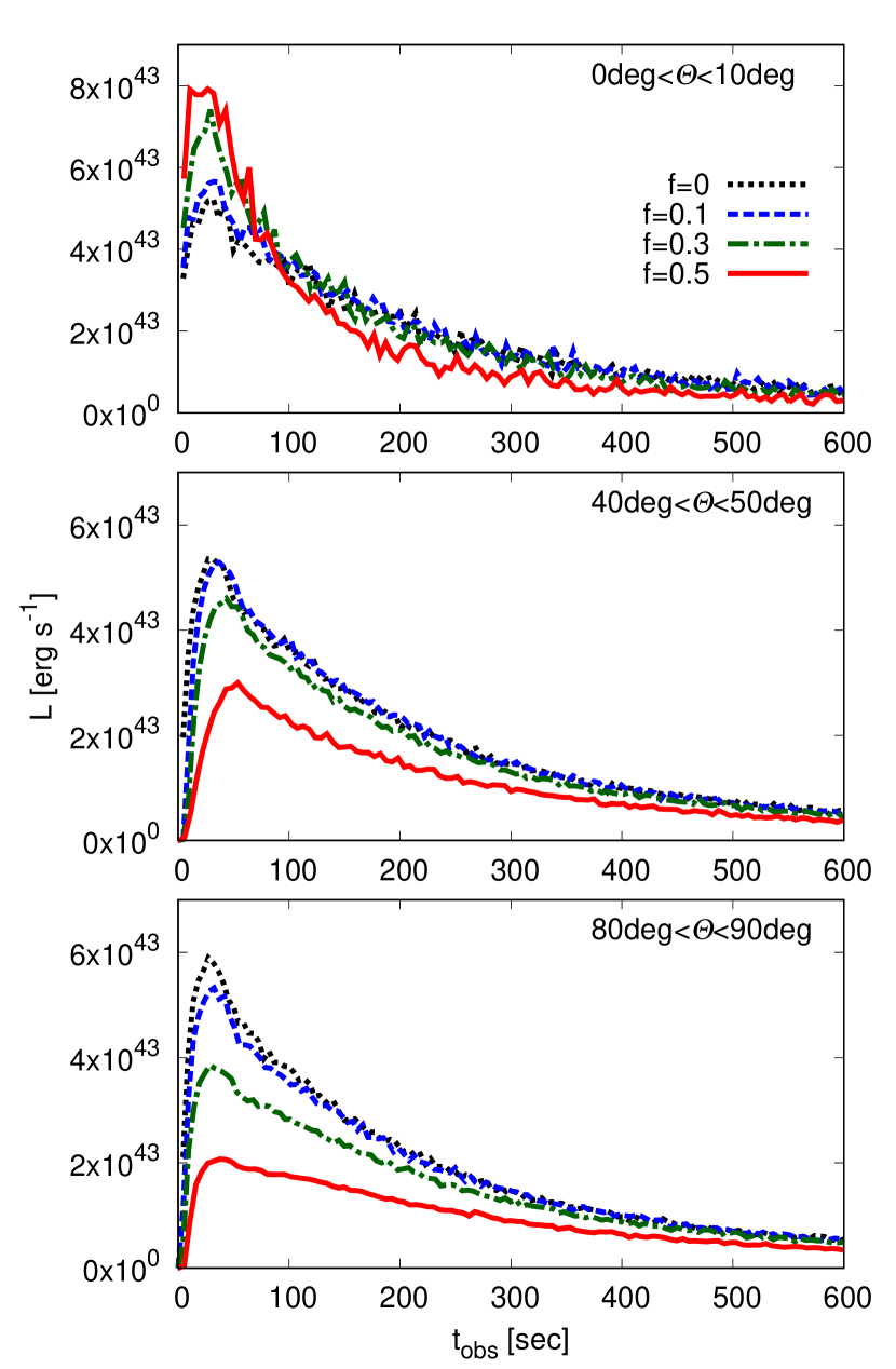
Figure 6.— Light curves (0.3–10 keV) of X-ray emission originating from ellipsoidal shocks. The graphs are shifted to the left side so that the times of onset corresponds to that for $f=0$.

Figure 6 shows the light curves in the energy range of the Swift/XRT when the shock has an oblateness of 0.1, 0.3, and 0.5. The time $t_{\rm obs}$ is measured from the moment when the first photon passes a large spherical surface concentric with the ejecta. In each panel, the flux is averaged over the angular ranges of $\theta=$[0,10], [40,50], and [80,90] deg, respectively. The light curves show that the timescales (the rise time and the duration) of the luminosity evolution have similar values regardless of $f$ and $\Theta$. As with the spherically symmetric case, the decay time of a few hundred sec is uniquely determined by the density distribution of the CSM. The reason of the similarity in the rise time is rather complicated. It depends on the shock velocity of which value varies with the inclination angle. When the radiation intensity is concentrated in a small angle ($<\theta_{\rm rel}$), the rise time $\theta_{\rm rise}$ becomes significantly shorter than the light crossing time $\Delta t_{\rm lc}$ of the size of the emerging shock, while when the intensity is broadly distributed ($v=0.5c$ in Figure 7), $\Delta t_{\rm rise}$ roughly equals to $\Delta t_{\rm lc}$. For example, we can estimate the rise time observed with a viewing angle of $\Theta=0$ for a shock with an oblateness of $f=0.5$. The high shock velocity along the line of sight $\sim 0.8c$ implies that most photons reaching an observer travel close to the symmetry axis ($\theta<30$ deg) due to beaming effects (see Figure 7). Thus the rise time is approximated as $[R_{b,\theta=0}-R_{b,\theta=30^{\circ}}\cos 30^{\circ}]/c\sim 40$ sec where $R_{b,\theta=0}=4\times 10^{12}$ cm and $R_{b,\theta=30^{\circ}}=3\times 10^{12}$ cm. On the other hand, the rise time observed with a viewing angle $\Theta=90$ deg can be approximated by $\Delta t_{lc}=40$ sec because of the low shock velocity along the line of sight $\sim 0.5c$.

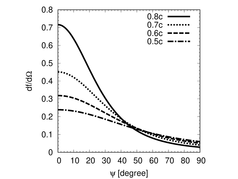
Figure 7.— Angular distribution of photons generated from the shock with a velocity of $0.8c$, $0.7c$, $0.6c$, $0.5c$ in the observer frame. The integral over the solid angle $\Omega$ becomes unity.

The peak luminosity $L_{\rm peak}$ decreases with $\Theta$, as well as the velocity of the shock propagating along the line of sight. The relation between the shock velocity $v$ and $L_{\rm peak}$ in the energy range of 0.3–10 keV is displayed in Figure 8. The bin widths of $v$ correspond to the ranges of the viewing angle $\Theta$. Within the range of $0.4c\lesssim v\lesssim 0.8c$, the values of $L_{\rm peak}$ tends to increase with increasing $v$ due to the bulk-Comptonization. For a lower shock velocity, such a positive correlation would become weaker because photons cannot gain much energy from electrons via electron scattering. Figure 9 shows the light curves for the energy lower than 0.3 keV. Again, all of the models have similar results in the timescales and the overall evolution of the luminosity due to the simultaneous shock breakouts in all directions. Thus the timescales responsible for the shape of the light curve becomes independent of the oblateness of the shock and the viewing angle. Consequently, from such a light curve it would be possible to know whether the morphology of the CSM is spherical and the velocity of the shock propagating along the line of sight. On the other hand, it would be difficult to constrain the degree of asphericities of the ejecta and shock front.

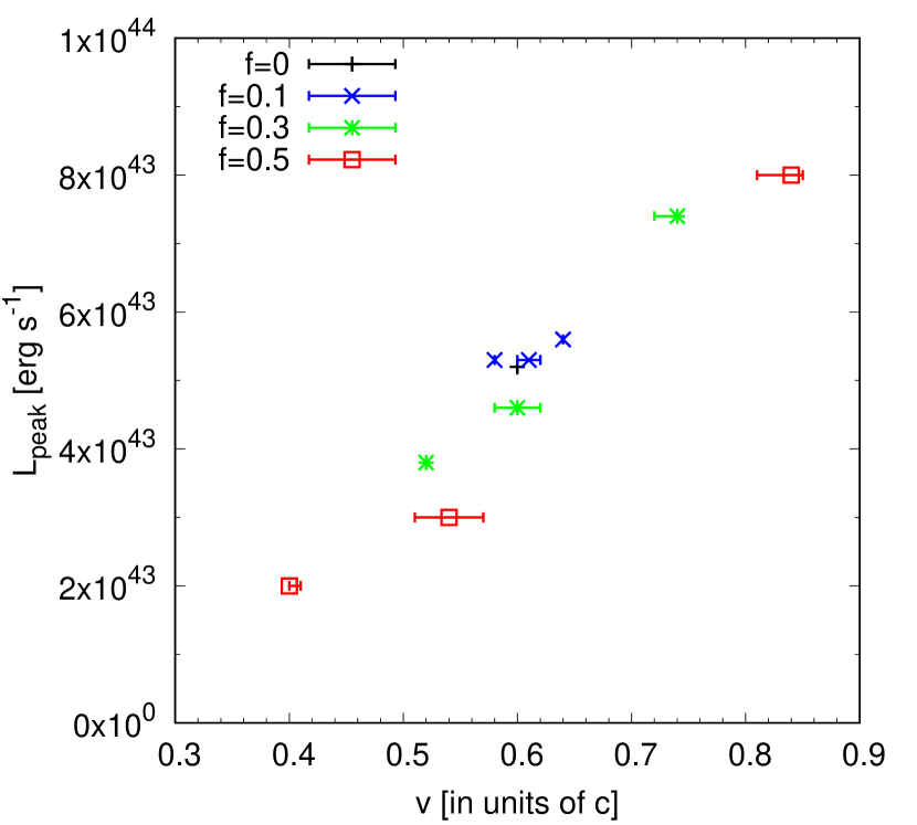
Figure 8.— Correction between the shock velocity and the peak luminosity. The errors shown in the horizontal bars are caused by the angular width of $\Theta$ (=[0,10], [40,50], and [80,90])

.

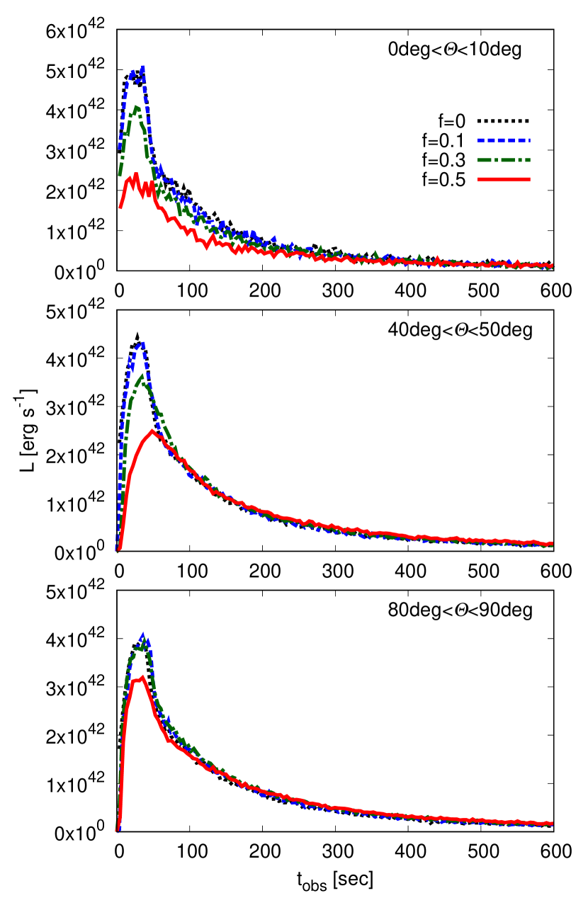
Figure 9.— The same as Figure 6 but for energies below 0.3 keV.

Figure 10 shows the time-integrated spectra for $f=$0.1, 0.3, and 0.5. When the shock front has a finite oblateness, the power-law gradient of the high energy (1–7 keV) component is shallower along the on-axis compared to the spherically symmetric case, while it is much steeper along the off-axis. This is because the shock has the radial velocity higher than $0.6c$ in the vicinity of the axis and lower at off-axis. Consequently, the influence of bulk-Comptonization becomes weaker as $\Theta$ becomes larger.

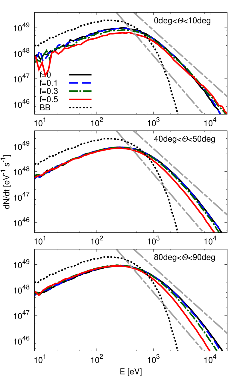
Figure 10.— Time-integrated spectra of X-ray emission originated from an axisymmetric shock. The dashed curve represents a blackbody spectrum at a temperature of $k_{\rm B}T_{\rm b}$. The gradients of the straight lines are -2.0 and -2.6, which correspond to the $\pm 1\sigma$ values of those of the observed Swift/XRT spectrum.

We compare the calculation for the ellipsoidal shock wave with XRO 080109. Figure 11 shows the light curve for $f=0.5$ and $\Theta=$45 deg as our best model. The overall shape of the light curve is roughly consistent with observation. In fact, an off-axis line of sight has also been suggested for XRO 080109 from late-phase observations of nebular emission lines of SN 2008D (Tanaka et al., 2009a), and our results are consistent with this interpretation. As shown in Figure 10, the high-energy spectral gradient is within a $1\sigma$ error range of the observation if the shock velocity along the line of sight is higher than $\sim 0.5c$.

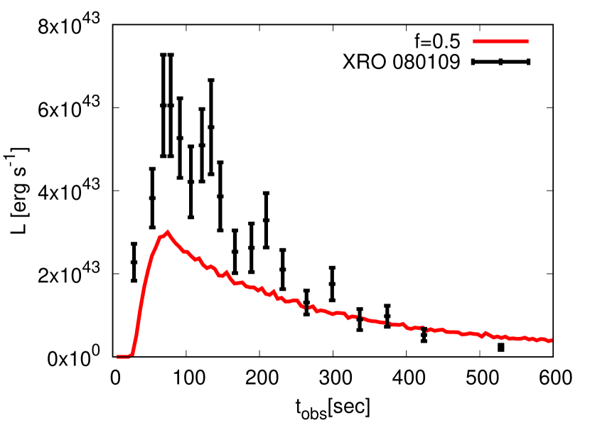
Figure 11.— The same as Figure 3 but for an ellipsoidal shock with an oblateness of $f=0.5$.

4. Conclusions

We investigate the properties of X-ray emission from shock breakout in a dense CSM. For this purpose, we calculate transfer of X-ray photons interacting with matter through Compton scattering and free-free absorption by using a Monte-Carlo method. We also study relations between the asphericity of the shape of the ellipsoidal shock front and the observational features of the emission.

The rise time of the light curve $\Delta t_{\rm rise}$ is mainly determined by the light crossing time $\Delta t_{\rm lc}$ of the breakout radius and also slightly affected by the diffusion time $t^{\prime}_{\rm diff}$ of photons in the shocked CSM. The major factor determining the duration of the light curve is the light crossing time of the radius at which photons last scatter off electrons. Even for an aspherical explosion, the properties of the light curve, such as the duration, the rise time, and the shape of the declining part, do not dramatically depend on the viewing angle as long as a steady and spherically symmetric wind is considered. The result suggests that the characteristics of the light curve are a good probe of the CSM density or mass loss rate.

We show that both of the observed light curve and spectrum of XRO 080109/SN 2008D can be reproduced by mildly-relativistic shock breakout in a dense spherical CSM. For a shock with the velocity of $0.6c$ and CSM with a mass loss rate of $5\times 10^{-4}M_{\odot}$ yr^-1, the rise time, the duration and the shape of the calculated X-ray light curve can be consistent with the observation. The power-law spectral gradient of the observed emission is also reproduced if the shock propagates toward the observer at a speed greater than $\sim 0.5c$.

Appendix A Relation of shock velocity to oblateness

The shape of the shock front should be changed under a fixed value of the explosion energy $E_{\rm kin}$. In the following few equations, we approximate the velocity of ejecta by that of the shock front. Here we define a typical time $t_{\rm b0}$ for each model, at which the mass density $\rho_{\rm ej}$ of ejecta has the same value as the moment of shock breakout for $f=0$. $t_{\rm b0}$ equals $(1-f)^{-2/3}t_{\rm i}$ where $t_{\rm i}$ denotes the moment of shock breakout along the symmetric axis. Then $E_{\rm kin}$ and the total ejecta mass $M_{\rm ej}$ are roughly expressed by the following equations.

$$E_{\rm kin} \approx \iiint\dfrac{\rho_{\rm ej0}v^{2}(f,\theta)}{2}r^{2}\sin\theta drd\theta d\phi$$ (A1)

$$= \dfrac{\pi\rho_{\rm ej0}v^{2}_{0}}{3}\int^{\pi}_{0}\left[\dfrac{R^{3}(1-f)^{2}\sin\theta}{(1-f)^{2}\cos^{2}\theta+\sin^{2}\theta}\right]d\theta$$

$$= \dfrac{2\pi\rho_{\rm ej0}v^{2}_{0}R^{3}_{0}}{9}\cdot(2f^{2}-4f+3)(1-f)^{2},$$

$$M_{\rm ej} = \dfrac{4\pi\rho_{\rm ej0}R^{3}_{0}}{3}(1-f)^{2},$$ (A2)

where $\phi$ is the azimuth angle, $R$ the shock radius, and $\rho_{\rm ej0}$, $v_{0}$ and $R_{0}$ are the values at $\theta=0$. Accordingly,

$$E_{\rm kin}\propto v^{2}_{0}\times(2f^{2}-4f+3)$$ (A3)

As a result, with a fixed $v_{f=0}=0.6c$, $v_{0}$ can be written by Equation (2).

Appendix B Collision of the spherically symmetric ejecta with power-law density and the circumstellar matter

In order to see if the assumption of uniform density significantly influences on the results of the calculation, we make a calculation for spherically symmetric ejecta with a power-law density ($\propto r^{-n}$). The issue of the absolute luminosity is beyond the scope of this work. We describe the hydrodynamics by using the Chevalier self-similar solution. We examine the emission for $n=10$, 12 and 7 (ordinarily used to describe type Ia SNe).

B.1. Settings

To calculate the X-ray light curve and spectra, we describe the spherically symmetric distribution of the shocked matter and freely-expanding ejecta as follows.

The structure of the shocked CSM is determined by Parker (1963), in which the radius of the forward shock $R_{1}$ increases with time $t$ as $R_{1}\propto t^{1/\lambda_{\rm fr}}$ ($\lambda_{\rm fr}$: constant). In the stationary CSM, if $\lambda_{\rm fr}=3/2$, the total energy of the shock becomes constant. Here we assume the same density profile of the unshocked CSM and the shock radius $R_{1}$ at the moment of breakout as those ($n_{1}$ and $R_{{\rm b},{f=0}}$) in Section 2.1.

The structure of the shocked ejecta is derived by Chevalier (1982), in which the density of the unshocked ejecta is assumed by

$$\rho_{\rm ej}=t^{-3}\left(\dfrac{r}{tg}\right)^{-n}.$$ (B1)

($g$, $n$: constant) and the radius $R_{2}\propto t^{1/\lambda_{\rm rv}}$ of the reverse shock, where $\lambda_{\rm rv}=(n-2)/(n-3)$. Noting that the pressure and velocity of the shocked matter should be continuous at the contact surface, $g$ becomes $4.6\times 10^{9}$ for $n=7$, $7.6\times 10^{9}$ for $n=10$ and $9.0\times 10^{9}$ for $n=12$. Figure 12 displays the fluid profile.

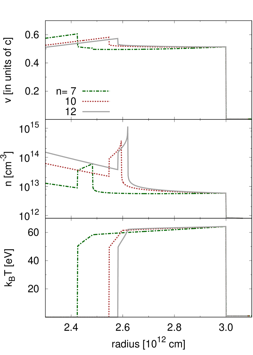
Figure 12.— Velocity, number density and temperature at the time of shock breakout. The density of the unshocked CSM and ejecta is assumed to have power-law distribution.

Using the hydrodynamical profile above, the X-ray light curves and time-integrated spectra for the fixed shock velocity $0.6c$ at the moment of shock breakout are calculated. The settings for the Monte-Carlo calculation is the same as those in Section 2.2 with the exception of the following. If the velocity of the forward shock is fixed at $0.6c$ at the moment of shock breakout, $t_{\rm b}$ becomes 133 sec for $n=7$, 146 sec for $n=10$, and 150 sec for $n=12$. The temperature of the matter is 64 eV (hereafter $k_{\rm B}T_{2,{\rm ch}}$) at the shock front. From the electron number density $n_{\rm ej}$ of $\approx 10^{14}$ cm^-3 in the ejecta and temperature $T$ of $T_{2,{\rm ch}}$, the total emissivity of free-free emission $\varepsilon^{\rm ff}_{\nu}$ is estimated to be $\approx 10^{5}$ erg s^-1 cm^-3 and the energy $E^{\rm ff}_{\nu}$ radiated from the ejecta per unit time $\approx 10^{43}$ erg s^-1. Therefore it takes $\approx 10^{2}$–$10^{3}$ sec to release the energy of $E_{\rm tot,i}$. The fact would not lead conclusion that it is impossible to generate photons by free-free emission, but a more careful study would be needed to discuss the structure of the shock in detail.

B.2. Light curves and spectra

We investigate how the shapes of the light curve and X-ray spectrum differ from those in calculated in Section 3. For example, if the density of the shocked matter follows a uniform distribution, the rise time $\Delta t_{\rm rise}$ strongly depends on the light crossing time $\Delta t_{\rm lc}$ of the breakout radius and weakly on diffusion time $t^{\prime}_{\rm diff}$. Here we investigate the dependence of the emission properties on the structure of the shock in spherically symmetric case.

Figure 13 shows the resultant light curves in the energy range of 0.3–10 keV. The graphs are compared with the model with uniform density distribution (black dotted line; the luminosity is scaled by a factor of 0.05). If $n=10$ and 12, the overall shapes of the light curves are quite similar to that for the model with uniform density. In order to know on what timescales the rise time $\Delta t_{\rm rise}$ and duration depend, we compare the diffusion time $t^{\prime}_{\rm diff}=(R^{\prime\prime}_{\tau=1}-r_{\rm min})/v$ in the shocked matter and unshocked CSM, and the light crossing time $\Delta t_{\rm lc}$ of the size of the emerging shock. Here $R^{\prime\prime}_{\tau=1}\sim 7\times 10^{12}$ cm. From the radius $r_{\rm min}$ (which satisfies $\int^{R_{\rm c}}_{\rm rmin}\kappa\rho dr$=1), $2.58\times 10^{12}$ cm for $n=10$ and $2.61\times 10^{12}$ cm for $n=12$, $t^{\prime}_{\rm diff}$ is estimated to be $\sim(R^{\prime\prime}_{\tau=1}-r_{\rm min})/0.5c=300$ sec, which is longer than the light crossing $\Delta t_{\rm lc}$ estimated in Section 3.1. For this reason, $\Delta t_{\rm lc}$ can be said to be the primary factor in determining $\Delta t_{\rm rise}$ rather than $t^{\prime}_{\rm diff}$.

Though a model with $n=7$ is fainter than those with $n=10$ and $n=12$ due to the low temperature of the shocked matter, the timescale of the brightening and the duration are not significantly different from those with $n=10$ and 12. (The radius $r_{\rm min}$ equals $2.45\times 10^{12}$ cm so that $t^{\prime}_{\rm diff}>\Delta t_{\rm lc}$.)

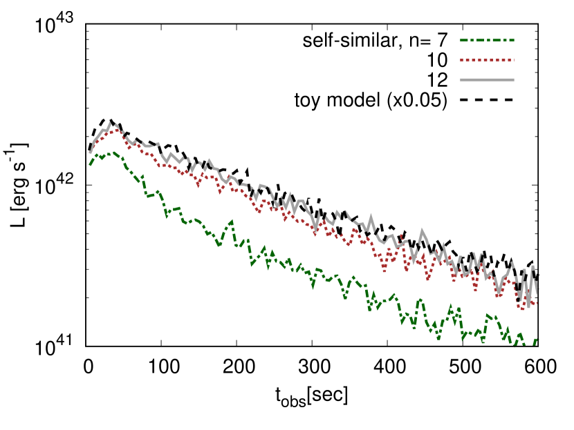
Figure 13.— Light curves (0.3–10 keV) calculated using the 1D Chevalier model. The black dashed line displays the solid line of Figure 3, scaled vertically by a factor of 0.05.

Figure 14 shows the time-integrated spectrum. Here we examine how the spectral gradient of the high-energy (1–7 keV) component changes with the motion of the matter. In comparison with the model with the uniform density and velocity distribution (black short-dotted line), the spectral gradient is steeper if the structure behind the shock is considered. It is because the velocity of the shocked matter is lower than the shock wave. For Figure 14, we can say that the spectral gradient of the high-energy tail is determined by the effect of bulk-Comptonization, so it can be a source of information on the shock velocity.

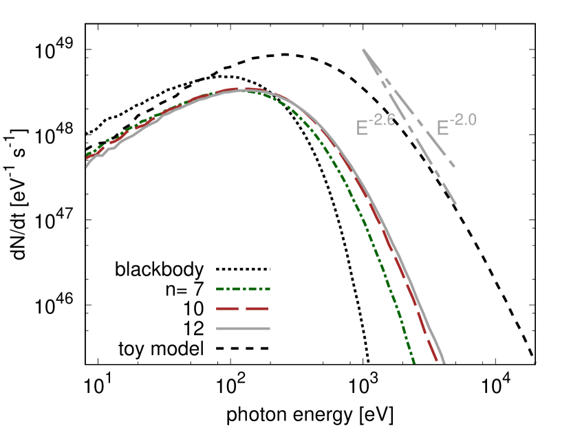
Figure 14.— Time-integrated spectra calculated using the 1D Chevalier self-similar solution for $n=7$, 10 and 12, and that of a blackbody at a temperature of $k_{\rm B}T_{2,{\rm ch}}$ (black dotted line). The black short-dashed line displays the solid curve of Figure 5.

References

- Balberg & Loeb (2011) Balberg, S., & Loeb, A. 2011, MNRAS, 414, 1715
- Campana et al. (2006) Campana, S., Mangano, V., Blustin, A. J., et al. 2006, Nature, 442, 1008
- Chevalier (1982) Chevalier, R. A. 1982, ApJ, 258, 790
- Chevalier & Fransson (2008) Chevalier, R. A., & Fransson, C. 2008, ApJ, 683, L135
- Chevalier & Irwin (2011) Chevalier, R. A., & Irwin, C. M. 2011, ApJ, 729, L6
- Chevalier & Irwin (2012) —. 2012, ApJ, 747, L17
- Couch et al. (2011) Couch, S. M., Pooley, D., Wheeler, J. C., & Milosavljević, M. 2011, ApJ, 727, 104
- Ensman & Burrows (1992) Ensman, L., & Burrows, A. 1992, ApJ, 393, 742
- Falk (1978) Falk, S. W. 1978, ApJ, 225, L133
- Hamann et al. (1995) Hamann, W.-R., Koesterke, L., & Wessolowski, U. 1995, A&A, 299, 151
- Herald et al. (2000) Herald, J. E., Schulte-Ladbeck, R. E., Eenens, P. R. J., & Morris, P. 2000, ApJS, 126, 469
- Humphreys & Davidson (1994) Humphreys, R. M., & Davidson, K. 1994, PASP, 106, 1025
- Katz et al. (2010) Katz, B., Budnik, R., & Waxman, E. 2010, ApJ, 716, 781
- Klein & Chevalier (1978) Klein, R. I., & Chevalier, R. A. 1978, ApJ, 223, L109
- Li (2008) Li, L.-X. 2008, MNRAS, 388, 603
- Maeder & Meynet (1987) Maeder, A., & Meynet, G. 1987, A&A, 182, 243
- Malesani et al. (2009) Malesani, D., Fynbo, J. P. U., Hjorth, J., et al. 2009, ApJ, 692, L84
- Matzner et al. (2013) Matzner, C. D., Levin, Y., & Ro, S. 2013, ApJ, 779, 60
- Matzner & McKee (1999) Matzner, C. D., & McKee, C. F. 1999, ApJ, 510, 379
- Mazzali et al. (2008) Mazzali, P. A., Valenti, S., Della Valle, M., et al. 2008, Science, 321, 1185
- Meynet et al. (1994) Meynet, G., Maeder, A., Schaller, G., Schaerer, D., & Charbonnel, C. 1994, A&AS, 103
- Modjaz et al. (2009) Modjaz, M., Li, W., Butler, N., et al. 2009, ApJ, 702, 226
- Moriya et al. (2011) Moriya, T., Tominaga, N., Blinnikov, S. I., Baklanov, P. V., & Sorokina, E. I. 2011, MNRAS, 415, 199
- Nakar & Sari (2010) Nakar, E., & Sari, R. 2010, ApJ, 725, 904
- Nugis et al. (1998) Nugis, T., Crowther, P. A., & Willis, A. J. 1998, A&A, 333, 956
- Ohtani et al. (2013) Ohtani, Y., Suzuki, A., & Shigeyama, T. 2013, ApJ, 777, 113
- Parker (1963) Parker, E. N. 1963,
- Prinja et al. (1990) Prinja, R. K., Barlow, M. J., & Howarth, I. D. 1990, ApJ, 361, 607
- Rybicki & Lightman (1979) Rybicki, G. B., & Lightman, A. P. 1979, Radiative processes in astrophysics
- Salbi et al. (2014) Salbi, P., Matzner, C. D., Ro, S., & Levin, Y. 2014, ApJ, 790, 71
- Seaton (1959) Seaton, M. J. 1959, MNRAS, 119, 81
- Soderberg et al. (2008) Soderberg, A. M., Berger, E., Page, K. L., et al. 2008, Nature, 453, 469
- Suzuki et al. (2016) Suzuki, A., Maeda, K., & Shigeyama, T. 2016, ApJ, 825, 92
- Suzuki & Shigeyama (2010a) Suzuki, A., & Shigeyama, T. 2010a, ApJ, 719, 881
- Suzuki & Shigeyama (2010b) —. 2010b, ApJ, 717, L154
- Svirski & Nakar (2014) Svirski, G., & Nakar, E. 2014, ApJ, 788, L14
- Svirski et al. (2012) Svirski, G., Nakar, E., & Sari, R. 2012, ApJ, 759, 108
- Tanaka et al. (2009a) Tanaka, M., Yamanaka, M., Maeda, K., et al. 2009a, ApJ, 700, 1680
- Tanaka et al. (2009b) Tanaka, M., Tominaga, N., Nomoto, K., et al. 2009b, ApJ, 692, 1131
- Wang et al. (2007) Wang, X.-Y., Li, Z., Waxman, E., & Mészáros, P. 2007, ApJ, 664, 1026