Large $N$ critical exponents for the chiral Heisenberg Gross-Neveu universality class

Abstract. We compute the large $N$ critical exponents $\eta$, $\eta_{\phi}$ and $1/\nu$ in $d$-dimensions in the chiral Heisenberg Gross-Neveu model to several orders in powers of $1/N$. For instance, the large $N$ conformal bootstrap method is used to determine $\eta$ at $O(1/N^{3})$ while the other exponents are computed to $O(1/N^{2})$. Estimates of the exponents for a phase transition in graphene are given which are shown to be commensurate with other approaches. In particular the behaviour of the exponents in $2$ $<$ $d$ $<$ $4$ is in qualitative agreement with a functional renormalization group analysis. The $\epsilon$-expansion of each exponent near four dimensions is in exact agreement with recent four loop perturbation theory.

LTH 1147

1 Introduction.

One of the more remarkable fundamental quantum field theories is the Gross-Neveu or Ashkin-Teller model, [1, 2]. It is a purely fermionic theory with a sole quartic self-interaction. In some sense it is the parallel to the more widely studied purely scalar quartic field theory which is renormalizable in four spacetime dimensions. The spontaneous symmetry breaking phase in that model is the basis for the Higgs mechanism of the Standard Model. By contrast the $O(N)$ Gross-Neveu model is asymptotically free, [1], but appears to have little physical application since it is only renormalizable in two dimensions. Put another way prior to the discovery of the $W$ and $Z$ vector bosons of the Standard Model the physics of the weak interactions was described by an effective field theory involving $4$-point fermion interactions. The restriction to being effective meant that such interactions could only be reliable as a model of Nature up to a specific momentum scale. However, the general Gross-Neveu class of quantum field theories, several of which were introduced in [1], have enjoyed a renaissance over recent years. This is in the main due to the fact that certain phase transitions in graphene can be described by specific universality classes based on the Gross-Neveu model, [1], where the classes derive from the underlying symmetry of the transition. For instance, stretching a graphene sheet can bring about a transition from a conductor to a Mott-insulating phase, [3, 4]. It has been suggested that the physics of this transition can be described by what is termed the chiral Heisenberg Gross-Neveu model, [5, 6, 7, 8, 9]. Therefore there has been activity in computing and estimating the fundamental critical exponents of the transition in this model. Prior to $2014$ there were virtually no deep computations where the theoretical status can be appreciated in the right panels of Figures $1$, $2$ and $3$ given in [9].

More specifically in [9] the critical exponents $\eta$, $\eta_{\phi}$ and $1/\nu$ were estimated in spacetime dimension $d$ where $2$ $<$ $d$ $<$ $4$ using functional renormalization group techniques. Hence values were given for the three dimensional case of physical interest to graphene. By contrast at that time only two loop $\epsilon$ expansion results from four dimensions were available to compare with, [10, 11]. Since then this four dimensional perturbative work has been extended to three and four loops respectively in [12, 13, 1]. The situation can be compared to the more widely studied Ising Gross-Neveu model which was given in the left panels of Figures $1$, $2$ and $3$ of [9]. By contrast with the chiral Heisenberg Gross-Neveu model in the Ising case there are now two dimensional $\epsilon$ expansion estimates to four loops, [15], as well as four loop four dimensional perturbative information, [11]. These higher loop results postdate the lower loop results of [1, 16, 17, 18, 19, 20, 21] which were the state of the art at the time of [9] for the Ising Gross-Neveu universality class. On top of this, Monte Carlo data, [11], as well as estimates from several orders in the large $N$ expansion, [22, 23, 24, 25, 26, 27, 28], were available to give independent analyses of the three dimensional exponents. Overall there was solid agreement for the exponents $\eta_{\phi}$ and $1/\nu$ from all these methods as well as the functional renormalization group analysis itself which was given in [9]. However those from the $\epsilon$ expansions near two and four dimensions for $\eta$ were not in close agreement with the other methods, [9]. One simple reason for this is clear from the plot for $\eta$ in Figure $1$ of [9]. It is because $\eta$ has to vanish in the limits down to two and up to four dimensions separately. So significantly higher orders in $\epsilon$ as well as knowledge of the asymptotic behaviour of the series would be required even to get close to the three dimensional estimates from the other methods.

A deeper underlying reason for this rests in the various theories which populate a universality class. Viewing the class as driven by a fundamental interaction at the Wilson-Fisher fixed point in $d$-dimensions, in the neighbourhood of an even spacetime dimension there is a quantum field theory which is renormalizable at that critical (even) dimension. Clearly it would not be renormalizable at another critical dimension. However a different theory would be relevant at that critical dimension but which will have the same fundamental interaction. In the case of the Ising Gross-Neveu universality class the theory which is renormalizable in two dimensions is the Gross-Neveu model of [1]. By contrast in four dimensions the next theory in the tower of theories at the Wilson-Fisher fixed point is what is termed the Gross-Neveu-Yukawa model, [29]. The respective Lagrangians differ only in the terms involving a scalar field. While we noted earlier that the Gross-Neveu model is purely fermionic, the quartic self-interaction can be rewritten via a scalar auxiliary field $\sigma$ to produce a $\sigma\bar{\psi}^{i}\psi^{i}$ interaction where $\psi^{i}$ are the fermions. This interaction is common to the Gross-Neveu-Yukawa model but the $\sigma$ field now has a canonical kinetic term and a scalar quartic self-interaction, [29]. It is this field $\sigma$ which has anomalous dimension $\eta_{\phi}$. Structurally the Gross-Neveu-Yukawa model has many similarities to the weak sector of the Standard Model itself. As noted in [9], for instance, this has led to the hope that certain phase transitions in graphene could mimic various symmetry breakings in the Standard Model itself such as chiral or spontaneous symmetry breaking. Currently experimental data from such graphene transitions are far from being available but the potential to have a simple laboratory to test Standard Model related phase transitions is a fascinating prospect. Other variations of the Gross-Neveu universality class are therefore becoming important to study so that precise theoretical predictions will be available.

Given the current sparcity of theoretical critical exponent estimates for the chiral Heisenberg Gross-Neveu model it is crucial to bring the analysis up to the same level of precision as that of the Ising Gross-Neveu universality class. By this we mean that the amount of precise data of the two classes as represented in Figures $1$, $2$ and $3$ of [9] should be the same for the different techniques used. This is the purpose of this article where we will compute the critical exponents $\eta$, $\eta_{\phi}$ and $1/\nu$ to the same order in the large $N$ expansion as those in the Ising universality class. This will be achieved by applying the critical point large $N$ formalism developed by Vasiliev et al in [30, 31, 32] for the $O(N)$ nonlinear $\sigma$ model or equivalently the $O(N)$ $\phi^{4}$ theory. Both these theories lie in the same universality class and the exponents of [30, 31, 32] are expressed as functions of $d$. That original approach was later extended to the Ising Gross-Neveu universality class in a series of articles, [22, 23, 24, 25, 26, 27, 28], and it is on a subset of these papers that the large $N$ computations presented here are based. For instance, for the most part we will analyse the basic $2$-point functions of the chiral Heisenberg Gross-Neveu theory by solving the skeleton Schwinger-Dyson equations algebraically in the limit as one approaches the $d$-dimensional Wilson-Fisher fixed point. While this will determine $\eta$, $\eta_{\phi}$ and $1/\nu$ to $O(1/N^{2})$, the original method given in [32] pointed the way to determining $\eta$ at $O(1/N^{3})$. This was extended to the Ising Gross-Neveu class in [24] and independently in [28]. Therefore, we will apply what we now term the large $N$ conformal bootstrap method to the chiral Heisenberg Gross-Neveu universality class. Given modern usage of the term conformal bootstrap method to mean a largely numerical technique based on solving the crossing symmetric $n$-point functions with manifest conformal symmetry, we have appended the term large $N$ to the naming of the earlier technique given in [32]. The work of [32] was inspired by the direct three dimensional conformal bootstrap construction of Parisi, [33], upon which the modern bootstrap, [34, 35, 36, 37], is also based.

The advantage of the approach of [30, 31, 32] is that the expression for $\eta$ at $O(1/N^{3})$ as well as the other exponents at $O(1/N^{2})$ are determined as exact functions of $d$. It is important to appreciate that this arbitrary spacetime dimension is not the same as the one used for dimensional regularization in perturbation theory. In [30, 31, 32] the skeleton Schwinger-Dyson equations are analytically and not dimensionally regularized. Therefore the exponents derived in the large $N$ method correspond to the exponents of the true theory at the Wilson-Fisher fixed point in arbitrary (non-integer) dimensions. Having said this the $\epsilon$ expansion of the large $N$ exponents around two or four dimensions are in exact agreement with the $\epsilon$ expansion of the perturbative critical renormalization group functions, evaluated at the fixed point, of the underlying theory with a critical dimension of two or four respectively. One benefit of having the exponents as functions of $d$ is that we will be able to plot their behaviour in $2$ $<$ $d$ $<$ $4$ dimensions which will provide an independent insight into whether the dependence on $d$ is consistent with that given by the functional renormalization group approach of [9] which used a sharp regulator. While three dimensional estimates are clearly and ultimately of physical interest the non-integer dimension structure of a field theory in effect is indicating the properties of the underlying universality class. In the context of the Standard Model these simple Ising Gross-Neveu and chiral Heisenberg Gross-Neveu classes may be pointing us to a novel way of viewing four dimensional physics. For instance, the observation that supersymmetry can emerge at a fixed point in a multicoupling quantum field theory, [38, 39, 40], may be directing us to a new era of beyond the Standard Model analyses. In other words the couplings of the relevant operators with Standard Model symmetries may flow to a fixed point which is accessed by an effective quantum field theory in the short term. However this could be superseded by a new one in much the same way as the Lagrangian introducing the $W$ and $Z$ vector bosons was eventually constructed. Therefore, exploring this new chiral Heisenberg Gross-Neveu universality class and understanding it in the graphene context offers new exciting avenues to explore.

The article is organized as follows. The following section introduces the chiral Heisenberg Gross-Neveu universality class together with the basic large $N$ formalism which will be used to extract the critical exponents to several orders in $d$-dimensions. In section $3$ the exponent $\eta$ is determined at $O(1/N^{2})$ and the evaluation of $\eta_{\phi}$ and $1/\nu$ to the same order are provided in sections $4$ and $5$ respectively. While these computations in essence follow the same critical point approach using the skeleton Schwinger-Dyson equations, the computation of $\eta$ at $O(1/N^{3})$ uses the large $N$ conformal bootstrap method which is outlined in section $6$. The analysis of our results is given in section $7$ where estimates are shown for the case of graphene and plots of the large $N$ exponents in $d$-dimensions are given for the Ising, XY and chiral Heisenberg Gross-Neveu models. Finally, we give our conclusions in section $8$.

2 Background.

The chiral Heisenberg Gross-Neveu model (cHGN) is a generalization of the original two dimensional $O(N)$ or $SU(N)$ Gross-Neveu model of [1] but where the $4$-point interaction is modified to include the three $SU(2)$ Pauli spin matrices $\sigma^{a}$ where $a$ $=$ $1$, $2$ and $3$. The Lagrangian is

$$L^{\mbox{\footnotesize{cHGN}}}~{}=~{}i\bar{\psi}^{i}\partial\!\!\!/\psi^{i}~{}+~{}\frac{g^{2}}{2}\left(\bar{\psi}^{i}\sigma^{a}\psi^{i}\right)^{2}$$ (2.1)

where $1$ $\leq$ $i$ $\leq$ $N$ and $g$ is the dimensionless coupling constant. Throughout our large $N$ computations we will use the spinor trace convention that $\mbox{Tr}I$ $=$ $2$ rather than $4$ which is ordinarily used when extending four dimensional perturbation theory to three dimensions. In other words to circumvent this convention we can rewrite our definition of $N$ using

$$N~{}=~{}\frac{1}{2}d_{\gamma}N$$ (2.2)

where $d_{\gamma}$ corresponds to the trace convention of the $\gamma$-matrices, [9]. The theory (2.1) is only perturbatively renormalizable in two dimensions. In four dimensions a quartic fermion interaction is non-renormalizable but (2.1) can be reformulated in terms of an auxiliary field $\tilde{\pi}^{a}$

$$L^{\mbox{\footnotesize{cHGN}}}~{}=~{}i\bar{\psi}^{i}\partial\!\!\!/\psi^{i}~{}+~{}g\tilde{\pi}^{a}\bar{\psi}^{i}\sigma^{a}\psi^{i}~{}-~{}\frac{1}{2}\tilde{\pi}^{a}\tilde{\pi}^{a}~{}.$$ (2.3)

In this formulation one can connect the original quartic interaction in the two dimensional theory with one in four dimensions which we will term the chiral Heisenberg Gross-Neveu-Yukawa (cHGNY) theory which has the Lagrangian

$$L^{\mbox{\footnotesize{cHGNY}}}~{}=~{}i\bar{\psi}^{i}\partial\!\!\!/\psi^{i}~{}+~{}\frac{1}{2}\partial_{\mu}\tilde{\pi}^{a}\partial^{\mu}\tilde{\pi}^{a}~{}+~{}g_{1}\tilde{\pi}^{a}\bar{\psi}^{i}\sigma^{a}\psi^{i}~{}+~{}\frac{1}{24}g_{2}^{2}\left(\tilde{\pi}^{a}\tilde{\pi}^{a}\right)^{2}~{}.$$ (2.4)

The sharing of the common Yukawa interaction in (2.3) and (2.4) is related to the fact that these theories are in the same universality class at their respective Wilson-Fisher fixed points. The bosonic sectors are different but they play a role in ensuring each Lagrangian is renormalizable in their respective critical dimensions. While both theories lie in the same universality class there is an underlying universal theory within which one can carry out computations in the large $N$ expansion. Specifically $d$-dimensional critical exponents can be determined to several orders in $1/N$, when $N$ is large, using methods based on [30, 31, 32]. These exponents encode all orders perturbative information on renormalization group functions in $d$-dimensions and hence contain information on all theories, such as (2.3) and (2.4), in the universality class in their critical dimension. The Lagrangian for the application of the large $N$ method to the underlying universal theory is

$$L~{}=~{}i\bar{\psi}^{i}\partial\!\!\!/\psi^{i}~{}+~{}\pi^{a}\bar{\psi}^{i}\sigma^{a}\psi^{i}~{}-~{}\frac{1}{2g}\pi^{a}\pi^{a}$$ (2.5)

where the field $\tilde{\pi}^{a}$ has been rescaled so that there is no coupling constant in the interaction. The method developed in [30, 31, 32] relies on the fact that at criticality it is the interaction which drives the dynamics at all scales. In comparison to (2.4) there is no quartic interaction. This is not an issue since the structure of the universal theory as such generates the requisite information corresponding to the critical renormalization group functions of (2.4) via $\pi^{a}$ $4$-point subgraphs in Feynman diagrams. This has been elucidated in [40] in the context of the large $N_{\!f}$ expansion of Quantum Chromodynamics (QCD) where $N_{\!f}$ is the number of massless quark flavours. Equally for other theories in the tower of this universality class the higher $\pi^{a}$ $n$-point subgraphs will contain the vertex structure of the higher $n$-point interactions relevant to the theory in a particular higher critical dimension.

The large $N$ critical point formalism of [30, 31, 32] exploits properties of the renormalization group at criticality to provide a method of solving the Schwinger-Dyson equations algebraically. In particular in the approach to a fixed point there is no scale aside from the correlation length. So, for instance, the propagators take an asymptotic scaling form whose behaviour is governed solely by the full dimension of the field. Specifically in coordinate space the scaling forms of the fermion and boson fields of (2.5) are, [22],

$$\psi(x)~{}\sim~{}\frac{Ax\!\!\!/}{(x^{2})^{\alpha}}~{}~{}~{},~{}~{}~{}\pi(x)~{}\sim~{}\frac{C}{(x^{2})^{\gamma}}$$ (2.6)

at leading order in the limit as $x$ $\to$ $0$ where we use the name of the field for each form. The quantities $A$ and $C$ are $x$-independent amplitudes and $\alpha$ and $\gamma$ are the full dimensions of the actual fields in the $d$-dimensional Lagrangian. These comprise the canonical dimension and the anomalous dimension. The former is deduced from ensuring that the dimension of each term in the Lagrangian is consistent with the action being dimensionless and we define

$$\alpha~{}=~{}\mu~{}+~{}\mbox{\small{$\frac{1}{2}$}}\eta~{}~{}~{},~{}~{}~{}\gamma~{}=~{}1~{}-~{}\eta~{}-~{}\chi_{\pi}$$ (2.7)

in parallel with [22] where $\eta$ is the anomalous critical exponent of the fermion. The anomalous dimension of $\pi^{a}$ includes $\eta$ and is derived from the Yukawa interaction where $\chi_{\pi}$ is the anomalous dimension of the Yukawa vertex itself. Here we use the convention of [30, 31] that the spacetime dimension $d$ is written as $d$ $=$ $2\mu$ for shorthand. In order to be able to compare with the critical exponent of the analogous bosonic field of [12, 14] we note that the corresponding exponent, $\eta_{\phi}$, is related to that of the $\pi^{a}$ field here by

$$\eta_{\phi}~{}=~{}4~{}-~{}2\mu~{}-~{}2(\eta~{}+~{}\chi_{\pi})~{}.$$ (2.8)

In terms of the connection with the renormalization group functions, $\eta$ corresponds to the fermion anomalous dimension evaluated at the Wilson-Fisher fixed point. As there is only one interaction the amplitudes $A$ and $C$ always appear in the same combination which we will denote by $y$ $=$ $A^{2}C$. It like all the critical exponents will only depend on $\mu$ and $N$ at criticality. Hence they can be expanded in powers of $1/N$ via

$$\eta(\mu)~{}=~{}\sum_{n=1}^{\infty}\frac{\eta_{n}(\mu)}{N^{n}}~{}~{}~{},~{}~{}~{}y(\mu)~{}=~{}\sum_{n=1}^{\infty}\frac{y_{n}(\mu)}{N^{n}}$$ (2.9)

and a similar notation will be used for other exponents. In (2.9) and similar expressions one can restore other spinor trace conventions by replacing $N$ with the definition (2.2). As we will be providing various critical exponents we need to recall the background formalism for those. While (2.6) gives the dominant behaviour of the propagators in the approach to criticality corrections to scaling can be included and for the propagators these take the form, [22],

$$\psi(x)~{}\sim~{}\frac{Ax\!\!\!/}{(x^{2})^{\alpha}}\left[1+A^{\prime}(x^{2})^{\lambda}\right]~{}~{}~{},~{}~{}~{}\pi(x)~{}\sim~{}\frac{C}{(x^{2})^{\gamma}}\left[1+C^{\prime}(x^{2})^{\lambda}\right]$$ (2.10)

where an independent exponent $\lambda$ governs the scaling of the correction with $A^{\prime}$ and $C^{\prime}$ the respective associated $x$-independent amplitudes. In principle $\lambda$ can be any exponent but for the moment we will let it correspond to the critical slope of the $\beta$-function of the theory whose critical dimension in this universality class is two and hence corresponds to (2.1) or (2.3). The connection with the exponents of [14] is that $1/\nu$ $=$ $2\lambda$ and we note that the leading order canonical dimension of $\lambda$ is $\lambda_{0}$ $=$ $\mu$ $-$ $1$.

One of the main methods to determine the explicit values of the exponents to several orders in $1/N$ is to systematically solve order by order the skeleton Schwinger-Dyson $2$-point function for both fields in the approach to criticality. This will also include the corrections to scaling. In order to do this one needs the asymptotic scaling forms of the respective $2$-point functions. These are derived from the propagator forms by inverting the momentum space propagators. To do this we use the Fourier transform given in [30, 31] which is

$$\frac{1}{(x^{2})^{\alpha}}~{}=~{}\frac{a(\alpha)}{2^{2\alpha}}\int_{k}\frac{e^{ikx}}{(k^{2})^{\mu-\alpha}}$$ (2.11)

where

$$a(\alpha)~{}=~{}\frac{\Gamma(\mu-\alpha)}{\Gamma(\alpha)}~{}.$$ (2.12)

This produces the coordinate space $2$-point function asymptotic scaling forms

$$\psi^{-1}(x) \sim \frac{r(\alpha-1)x\!\!\!/}{A(x^{2})^{2\mu-\alpha+1}}\left[1-A^{\prime}s(\alpha-1)(x^{2})^{\lambda}\right]$$

$$\pi^{-1}(x) \sim \frac{p(\gamma)}{C(x^{2})^{2\mu-\gamma}}\left[1-C^{\prime}q(\gamma)(x^{2})^{\lambda}\right]$$ (2.13)

which include the scaling corrections. The amplitudes differ from the respective ones in the propagator forms and the various functions of the exponents are given by

$$p(\gamma) = \frac{a(\gamma-\mu)}{a(\gamma)}~{}~{}~{},~{}~{}~{}r(\alpha)~{}=~{}\frac{\alpha p(\alpha)}{(\mu-\alpha)}$$

$$q(\gamma) = \frac{a(\gamma-\mu+\lambda)a(\gamma-\lambda)}{a(\gamma-\mu)a(\gamma)}~{}~{}~{},~{}~{}~{}s(\alpha)~{}=~{}\frac{\alpha(\alpha-\mu)q(\alpha)}{(\alpha-\mu+\lambda)(\alpha-\lambda)}~{}.$$ (2.14)

In summary we have introduced the basic structure of the propagators and $2$-point functions for the large $N$ critical point analysis. This is sufficient to solve the skeleton Schwinger-Dyson equation at $O(1/N^{2})$ and determine $d$-dimensional expressions for $\eta_{1}$, $\eta_{2}$, $\chi_{\pi\,1}$, $\lambda_{1}$ and $\lambda_{2}$. The values of $\chi_{\pi\,2}$ and $\eta_{3}$ are deduced from solving $3$-point functions at criticality and the formalism for each will be discussed later.

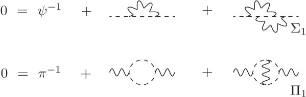
Figure 1: $O(1/N^{2})$ corrections to the skeleton Schwinger-Dyson $2$-point functions used to determine $\eta_{1}$ and $\eta_{2}$.

3 Evaluation of $\eta_{2}$.

As aspects of the solution of the $2$- and $3$-point functions for each of the various exponents are common we illustrate these features in more detail for the derivation of $\eta_{2}$. The first stage for this is to represent the skeleton Schwinger-Dyson $2$-point functions of Figure $1$ as algebraic equations. In coordinate space to $O(1/N^{2})$, which is sufficient to deduce $\eta_{1}$ and $\eta_{2}$, we have

$$0 = r(\alpha-1)~{}+~{}3yZ_{V}^{2}(x^{2})^{\chi_{\pi}+\Delta}~{}-~{}3y^{2}Z_{V}^{4}\Sigma_{1}(x^{2})^{2\chi_{\pi}+2\Delta}~{}+~{}O\left(\frac{1}{N^{3}}\right)$$

$$0 = p(\gamma)~{}+~{}2NyZ_{V}^{2}(x^{2})^{\chi_{\pi}+\Delta}~{}+~{}Ny^{2}Z_{V}^{4}\Pi_{1}(x^{2})^{2\chi_{\pi}+2\Delta}~{}+~{}O\left(\frac{1}{N^{2}}\right)$$ (3.1)

where we have substituted for the asymptotic scaling forms of the inverse propagators. The values of the respective two loop integrals $\Sigma_{1}$ and $\Pi_{1}$ are present and these not only depend on $N$ through the presence of the exponents on the internal lines but also on the regularization $\Delta$. This is introduced into the critical theory by shifting the anomalous dimension of the vertex via, [30, 31],

$$\chi_{\pi}~{}\rightarrow~{}\chi_{\pi}~{}+~{}\Delta$$ (3.2)

corresponding to an analytic regularization. Both graphs are divergent and can be represented by

$$\Sigma_{1}~{}=~{}\frac{K_{1}}{\Delta}~{}+~{}\Sigma_{1}^{\prime}~{}~{}~{},~{}~{}~{}\Pi_{1}~{}=~{}\frac{L_{1}}{\Delta}~{}+~{}\Pi_{1}^{\prime}$$ (3.3)

where the $O(\Delta)$ terms of the integrals would only become relevant for the $\eta_{3}$ derivation using this approach. As discussed in [30, 31] and [41] the core vertex is renormalized and this feature is present via the vertex renormalization constant $Z_{V}$ which also depends on $N$ and $\Delta$. It can be written as a double expansion via

$$Z_{V}~{}=~{}1~{}+~{}\sum_{l=1}^{\infty}\sum_{n=1}^{l}\frac{m_{ln}}{\Delta^{n}}$$ (3.4)

where the counterterms $m_{ln}$ are then expanded in powers of $1/N$

$$m_{ln}~{}=~{}\sum_{i=1}^{\infty}\frac{m_{ln,i}}{N^{i}}~{}.$$ (3.5)

Next an overall common factor of the length of the position vector $x^{2}$ has cancelled in (3.1). However, from the dimensionality of the Feynman graphs there is a remnant $x^{2}$ dependence deriving from the vertex anomalous dimension and the regularization. As it stands (3.1) is a formal representation of Figure $1$ but is not applicable in the scaling region, given by $x^{2}$ $\to$ $0$, where it ought to be independent of the length scale $x^{2}$. Equally the renormalization constant has to be determined as well as $\chi_{\pi}$. It turns out that all these issues are resolved together. To achieve this we formally substitute (3.3) and expand the factors involving $x^{2}$ to the appropriate orders in $1/N$ and $\Delta$ neglecting terms $O(1/N^{3})$ and $O(\Delta)$ respectively. To ensure that the algebraic Schwinger-Dyson equation is finite when the regularization is removed leads to

$$m_{11,1}~{}=~{}-~{}\frac{1}{4}y_{1}L_{1}$$ (3.6)

and the absence of $\ln x^{2}$ terms requires

$$\chi_{\pi\,1}~{}=~{}-~{}\frac{1}{2}y_{1}L_{1}~{}.$$ (3.7)

We have expressed these conditions in terms of the simple pole of the graph $\Pi_{1}$ rather than $\Sigma_{1}$. However similar relations emerge from the $\psi^{i}$ Schwinger-Dyson equation and these are not inconsistent since from explicit computation we have

$$K_{1}~{}=~{}-~{}\frac{1}{2}L_{1}$$ (3.8)

which ensures there are no ambiguous expressions for the vertex counterterm and $\chi_{\pi}$. The resulting Schwinger-Dyson equations

$$0 = r(\alpha-1)~{}+~{}3y~{}-~{}3y^{2}\Sigma_{1}^{\prime}~{}+~{}O\left(\frac{1}{N^{3}}\right)$$

$$0 = p(\gamma)~{}+~{}2Ny~{}+~{}Ny^{2}\Pi_{1}^{\prime}~{}+~{}O\left(\frac{1}{N^{2}}\right)$$ (3.9)

are now finite and independent of $x^{2}$ to the order in $1/N$ necessary to deduce $\eta_{1}$ and $\eta_{2}$.

To proceed one first concentrates on the leading order terms of both equations and eliminates $y_{1}$ to produce

$$p(\gamma)~{}=~{}\frac{2}{3}Nr(\alpha-1)~{}.$$ (3.10)

Setting the leading order value for $\gamma$ and $\alpha$ $=$ $\mu$ $+$ $\eta_{1}/N$ produces

$$\eta_{1}~{}=~{}-~{}\frac{3\Gamma(2\mu-1)}{\mu\Gamma(1-\mu)\Gamma(\mu-1)\Gamma^{2}(\mu)}~{}.$$ (3.11)

With this value established as well as that for the amplitude combination $y_{1}$ then $\eta_{2}$ is deduced by including the values of the finite parts of the two loop graphs and eliminating the unknown $y_{2}$. First, with

$$L_{1}~{}=~{}\frac{4}{(\mu-1)\Gamma^{2}(\mu)}$$ (3.12)

from [22] we find

$$\chi_{\pi\,1}~{}=~{}-~{}\frac{\mu}{3(\mu-1)}\eta_{1}$$ (3.13)

which is needed for the next term in the expansion of $p(\gamma)$. Then using

$$\Pi_{1}^{\prime}~{}=~{}-~{}\frac{4}{(\mu-1)^{2}\Gamma^{2}(\mu)}$$ (3.14)

from [22], where $\Sigma_{1}^{\prime}$ satisfies the same ratio with $\Pi_{1}^{\prime}$ as (3.8), we find

$$\eta_{2}~{}=~{}\left[\frac{(2\mu-3)}{3(\mu-1)}\Psi(\mu)~{}+~{}\frac{(4\mu^{2}-6\mu+1)}{2\mu(\mu-1)^{2}}\right]\eta_{1}^{2}$$ (3.15)

where we use the shorthand notation

$$\Psi(\mu)~{}=~{}\psi(2\mu-1)~{}-~{}\psi(1)~{}+~{}\psi(2-\mu)~{}-~{}\psi(\mu)$$ (3.16)

and $\psi(z)$ $=$ $d\ln\Gamma(z)/dz$ is the Euler $\psi$ function.

4 Evaluation of $\chi_{\pi\,2}$.

With the determination of the exponents of the last section we have obtained the critical behaviour of the $\psi^{i}$-field to $O(1/N^{2})$ and that of $\pi^{a}$ to $O(1/N)$. Since the asymptotic scaling forms of the inverse scaling functions, when there is correction to scaling, involve $\gamma$ then in order to find $\lambda$ at $O(1/N^{2})$ we need to find $\chi_{\pi\,2}$ first. One way is to determine the corrections to the skeleton $2$-point functions at next order in $1/N$. However this would involve a large amount of computation which would not be necessary since there is an alternative. The extraction of $\chi_{\pi\,1}$ from ensuring there are no terms involving $\ln x^{2}$ in the limit to criticality is reminiscent of a similar way of extracting the renormalization constant for a mass $m$ by renormalizing that part of a $2$-point function in conventional perturbation theory which corresponds to the wave function renormalization. By this we mean that in a renormalizable theory the one loop mass counterterm can be deduced from the two loop $2$-point wave function computation by ensuring that there are no non-renormalizable terms involving $\ln m^{2}$. While this is not the conventional way to extract such a one loop counterterm from a two loop evaluation it can be regarded in one way as a useful shortcut but more importantly as being consistent with the underlying renormalizability. The same process has in effect been played out in the finding $\chi_{\pi}$ at $O(1/N)$ through the computation of $\eta$ at $O(1/N^{2})$. While our discussion in the previous section followed the original algorithm outlined in [30, 31], the critical point large $N$ formalism was subsequently put in a parallel context to conventional perturbation theory in [41, 42]. The core aspects of perturbation theory are an ordering of the diagrams constituting a Green’s function and a regularization to facilitate their evaluation. With the ordering, such as the power of the coupling constant, the renormalization constants are introduced by multiplicative rescaling and determined with respect to a subtraction criterion. The situation developed in [41, 42] is completely parallel. Graphs are ordered with respect to the counting given by the power of $1/N$ with the regularization introduced by shifting the vertex anomalous dimension, [30, 31]. One major difference is that the residues of the poles in the renormalization constants are functions of the spacetime dimension $d$ which does not play a regularizing role. In this process the critical exponents are directly extracted in a renormalization group invariant way. In introducing the vertex renormalization constant $Z_{V}$ previously we were in effect following the $1/N$ renormalization formalism developed in [41, 42] which demonstrated that the ordering of graphs with a suitable regularization in effect was a complete parallel to conventional perturbation theory. Moreover it was shown in [41, 42] that the vertex anomalous dimensions, as well as operator renormalization, could be extracted from the critical point evaluation of $n$-point functions for $n$ $\geq$ $3$. Therefore to deduce $\chi_{\pi\,2}$ we follow that approach.

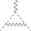
Figure 2: $O(1/N)$ graph to determine $\chi_{\pi\,1}$.

The first stage is to reproduce the value of $\chi_{\pi\,1}$ which requires the evaluation of the graph of Figure $2$. In this instance we use the momentum space asymptotic scaling forms for the propagators which are

$$\psi(p)~{}\sim~{}\frac{\tilde{A}p\!\!\!/}{(p^{2})^{\mu-\alpha+1}}~{}~{}~{},~{}~{}~{}\pi(p)~{}\sim~{}\frac{\tilde{C}}{(p^{2})^{\mu-\gamma}}$$ (4.1)

where $p$ is the momentum and $\tilde{A}$ and $\tilde{C}$ are the amplitudes in momentum space. However the combination $\tilde{y}$ $=$ $\tilde{A}^{2}\tilde{C}$ will always arise in the graphs. Its $O(1/N^{2})$ value is known via the Fourier transform (2.11) and we already have

$$\tilde{y}_{1}~{}=~{}-~{}\frac{y_{1}}{(\mu-1)\Gamma(\mu)}~{}~{}~{},~{}~{}~{}\tilde{y}_{2}~{}=~{}-~{}\frac{1}{(\mu-1)\Gamma(\mu)}\left[y_{2}~{}-~{}\frac{y_{1}\eta_{1}}{(\mu-1)}\right]$$ (4.2)

where from earlier calculations we can deduce

$$y_{1}~{}=~{}\frac{\mu}{6}\Gamma^{2}(\mu)\eta_{1}~{}~{}~{},~{}~{}~{}y_{2}~{}=~{}\left[\frac{\mu(2\mu-3)}{18(\mu-1)}\Psi(\mu)~{}+~{}\frac{\mu(5\mu-6)}{18(\mu-1)^{2}}\right]\Gamma^{2}(\mu)\eta_{1}^{2}~{}.$$ (4.3)

The approach to find the corrections to $\chi_{\pi}$ is similar to that of the $2$-point function. Once the graphs have been evaluated in momentum space to the finite part in $\Delta$ the contribution to the respective term of the exponent in $1/N$ is given by the coefficient of the $\ln p^{2}$ part. Such terms have to be absent in the limit to the critical point which then fixes the unknown exponent. Therefore following the prescription given in [41] we find the same expression for $\chi_{\pi\,1}$ as before.

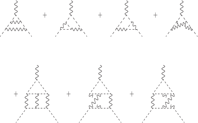
Figure 3: $O(1/N^{2})$ graphs to determine $\chi_{\pi\,2}$.

The computation to deduce $\chi_{\pi\,2}$ is more involved. The main part is the inclusion of the $O(1/N^{2})$ graphs of Figure $3$. These were evaluated in [23] for the parallel calculation of the vertex critical exponent in the $O(N)$ Gross-Neveu model. So for (2.5) the values of the master integrals are appended with the corresponding group theory factor. In addition there are next order contributions from the one loop graph of Figure $2$. This is because of the presence of $\eta$ and $\chi_{\pi}$ in the power of each of the propagators. In addition there are vertex counterterms from $Z_{V}$ for each vertex which have to be included in the same graph. They relate to the subgraph divergences arising from the first three graphs of the top row in Figure $3$. Piecing all the relevant contributions together and isolating the $\ln p^{2}$ part we find

$$\chi_{\pi\,2}~{}=~{}\left[-~{}\frac{\mu(2\mu-3)}{9(\mu-1)^{2}}\Psi(\mu)~{}-~{}\frac{\mu^{2}}{3\mu(\mu-1)}\Theta(\mu)~{}-~{}\frac{[14\mu^{3}-37\mu^{2}+31\mu-3]}{9(\mu-1)^{2}}\right]\eta_{1}^{2}~{}.$$ (4.4)

where

$$\Theta(\mu)~{}=~{}\psi^{\prime}(\mu)~{}-~{}\psi^{\prime}(1)~{}.$$ (4.5)

Equipped with $\chi_{\pi\,2}$ then both field anomalous dimensions are now available to the same order in $1/N$.

5 Evaluation of $\lambda_{2}$.

The next stage in the evaluation of the large $N$ critical exponents again mimics that of conventional perturbation theory in that with the wave function anomalous dimensions at $O(1/N^{2})$ one can establish the $\beta$-function to the same order. As noted earlier this is achieved by considering corrections to scaling and evaluating the corresponding $2$-point Schwinger-Dyson equations of Figure $1$ to the next order. There are various aspects of extracting the expansion for $\lambda$ which is not straightforward. Basic features are best illustrated by considering the equation for $\psi^{i}$ which can be represented by

$$0 = r(\alpha-1)\left[1-A^{\prime}s(\alpha-1)(x^{2})^{\lambda}\right]~{}+~{}3yZ_{V}^{2}(x^{2})^{\chi_{\pi}+\Delta}\left[1+\left(A^{\prime}+C^{\prime}\right)(x^{2})^{\lambda}\right]$$ (5.1)

$$-~{}3y^{2}Z_{V}^{4}(x^{2})^{2\chi_{\pi}+2\Delta}\left[\Sigma_{1}+\left(\Sigma_{1A}A^{\prime}+\Sigma_{1C}C^{\prime}\right)(x^{2})^{\lambda}\right]~{}+~{}O\left(\frac{1}{N^{3}}\right)$$

prior to renormalization. The two loop graph denoted by $\Sigma_{1}$ in Figure $1$ has been expanded to include the values where there is a correction to scaling in the $\psi^{i}$ and $\pi^{a}$ fields. These are $\Sigma_{1A}$ and $\Sigma_{1C}$ respectively and their values have been computed in [27]. The key difference with the inclusion of the corrections is that terms do not have the same dependence on $x^{2}$. This means that the equation decouples into two pieces. One is the piece which contributes to the determination of $\eta$ while the other involves the unknown $\lambda$ and is

$$0 = -~{}r(\alpha-1)s(\alpha-1)A^{\prime}~{}+~{}3yZ_{V}^{2}(x^{2})^{\chi_{\pi}+\Delta}\left[A^{\prime}+C^{\prime}\right]$$ (5.2)

$$-~{}3y^{2}Z_{V}^{4}(x^{2})^{2\chi_{\pi}+2\Delta}\left[\Sigma_{1A}A^{\prime}+\Sigma_{1C}C^{\prime}\right]~{}+~{}O\left(\frac{1}{N^{3}}\right)~{}.$$

Unlike the equation which determines $\eta$ the associated correction amplitudes are present linearly. If one ignores the contribution from the two loop graphs then the first two terms are the relevant ones for finding the value of $\lambda_{1}$. However there is a new feature in comparison with the corresponding equation to determine $\eta$. This is to do with the large $N$ dependence in that the first term is $O(1)$ while the second one is $O(1/N)$ which has an impact on the structure for the $\pi^{a}$ Schwinger-Dyson equation contributing to $\lambda$.

Turning to the second equation of Figure $1$ we can represent it in a similar way to that of the first equation and have

$$0 = p(\gamma)\left[1-C^{\prime}q(\gamma)(x^{2})^{\lambda}\right]~{}+~{}2NyZ_{V}^{2}(x^{2})^{\chi_{\pi}+\Delta}\left[1+2A^{\prime}(x^{2})^{\lambda}\right]$$ (5.3)

$$+~{}Ny^{2}Z_{V}^{4}(x^{2})^{2\chi_{\pi}+2\Delta}\left[\Pi_{1}+\left(\Pi_{1A}A^{\prime}+\Pi_{1C}C^{\prime}\right)(x^{2})^{\lambda}\right]~{}+~{}O\left(\frac{1}{N^{2}}\right)~{}.$$

The values of the two loop graphs with corrections to scaling on the $\psi^{i}$ and $\pi^{a}$ lines are $\Pi_{1A}$ and $\Pi_{1C}$ respectively. Again the equation decouples into that which determines $\eta$ and

$$0 = -~{}p(\gamma)q(\gamma)C^{\prime}~{}+~{}4NyZ_{V}^{2}(x^{2})^{\chi_{\pi}+\Delta}A^{\prime}$$ (5.4)

$$+~{}Ny^{2}Z_{V}^{4}(x^{2})^{2\chi_{\pi}+2\Delta}\left[\Pi_{1A}A^{\prime}+\Pi_{1C}C^{\prime}\right]~{}+~{}O\left(\frac{1}{N^{2}}\right)$$

which is formally similar to (5.2) and also includes the correction amplitudes $A^{\prime}$ and $C^{\prime}$. Between these two equations at leading order the only unknown is $\lambda_{1}$. The consistency equation which is formed to solve for it is deduced by first representing (5.2) and (5.4) as a matrix ${\cal M}$ given by

$${\cal M}~{}=~{}\left(\begin{array}[]{cc}-~{}r(\alpha-1)s(\alpha-1)&3y\\ 4Ny&-~{}p(\gamma)q(\gamma)~{}+~{}Ny^{2}\Pi^{\prime}_{1C}\\ \end{array}\right)$$ (5.5)

after renormalization where ^′ indicates the finite part of $\Pi_{1C}$ with respect to $\Delta$. It is worth noting that we have not retained all the terms in the Schwinger-Dyson equations in the matrix. This is because we want to concentrate on finding the value for $\lambda_{1}$ initially. Therefore we have retained the leading terms except for $\Pi^{\prime}_{1C}$ which would ordinarily be regarded as next order in the same way that the parent graph only contributed to $\eta_{2}$ and not $\eta_{1}$. The reason why this graph cannot be omitted resides in the powers of $N$ in the matrix, [27], and the fact that the consistency equation is given by requiring $\det({\cal M})$ $=$ $0$. Therefore in computing the determinant the two resultant terms have to be the same order in $1/N$. The complication arises from the scaling functions since

$$r(\alpha-1)s(\alpha-1)~{}=~{}O(1)~{}~{}~{},~{}~{}~{}p(\gamma)q(\gamma)~{}=~{}O\left(\frac{1}{N}\right)~{}.$$ (5.6)

Therefore both terms of the $(22)$ element are the same order in $1/N$ and the omission of $\Pi^{\prime}_{1C}$ would lead to an incorrect value of $\lambda_{1}$. Therefore setting

$$\Pi^{\prime}_{1C}~{}=~{}\Pi^{\prime}_{1C1}~{}+~{}\Pi^{\prime}_{1C2}\frac{1}{N}~{}+~{}O\left(\frac{1}{N^{2}}\right)$$ (5.7)

we have the leading order consistency equation

$$12y_{1}^{2}~{}-~{}r(\alpha-1)s(\alpha-1)\left[Np(\gamma)q(\gamma)~{}-~{}y_{1}^{2}\Pi_{1C1}\right]~{}=~{}0$$ (5.8)

where

$$q(\gamma)~{}=~{}\frac{1}{2(\mu-1)N}\left[\lambda_{1}-\eta_{1}-\chi_{\pi\,1}\right]~{}+~{}O\left(\frac{1}{N^{2}}\right)$$ (5.9)

to leading order. With, [27],

$$\Pi^{\prime}_{1C1}~{}=~{}\frac{2}{(\mu-1)^{2}\Gamma^{2}(\mu)}$$ (5.10)

we find

$$\lambda_{1}~{}=~{}-~{}(2\mu-1)\eta_{1}~{}.$$ (5.11)

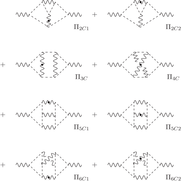
Figure 4: Graphs for $O(1/N^{2})$ correction to the $\pi^{a}$ skeleton Schwinger-Dyson $2$-point function to determine $\lambda_{2}$.

Having outlined in detail the formalism and issues behind the derivation of the leading order consistency equation for $\lambda_{1}$ we extend the analysis to the next order in $1/N$. Virtually all aspects of the Schwinger-Dyson equations discussed so far are sufficient to formally deduce the correction to the consistency equation defined by $\det({\cal M})$ $=$ $0$. For instance, the contributions from the two loop graph of the $\psi^{i}$ equation in Figure $1$ need to be included. However, for the $\pi^{a}$ equation there are two main additions. The first is that the appearance of $\Pi_{1C}$ at leading order means that the next term in its large $N$ expansion needs to be included as noted in (5.7) and the correction has the value, [27],

$$\Pi^{\prime}_{1C2}~{}=~{}\frac{2}{(\mu-1)^{2}\Gamma^{2}(\mu)}\left[\frac{3}{2}(\mu-1)\left[\eta_{1}-\chi_{\pi\,1}-\lambda_{1}\right]\left[\Theta(\mu)+\frac{1}{(\mu-1)^{2}}\right]-\frac{2}{(\mu-1)}\eta_{1}\right]~{}.$$ (5.12)

Also as another direct consequence of the presence of $\Pi_{1C}$ at leading the $O(1/N^{2})$ corrections to the $\pi^{a}$ Schwinger-Dyson equation have to be included. These are illustrated in Figure $4$ where the dot on a $\pi^{a}$ line denotes which line has the correction to scaling term. The values of the integrals were given in [27] but in this case the group factors have to be appended. We use a labelling of the graphs which is parallel to that used in [27]. Moreover their contribution has to be included in the extension of (5.4). If we denote the sum of the contributions from the graphs of Figure $4$ by $\Pi_{2C}$ then the extension of (5.5) is

$${\cal M}~{}=~{}\left(\begin{array}[]{cc}-~{}r(\alpha-1)s(\alpha-1)~{}+~{}3y&3y~{}-~{}3y^{2}\Sigma^{\prime}_{1C}\\ 4Ny~{}+~{}Ny^{2}\Pi^{\prime}_{1A}&-~{}p(\gamma)q(\gamma)~{}+~{}Ny^{2}\Pi^{\prime}_{1C}~{}+~{}\Pi_{C2}\\ \end{array}\right)~{}.$$ (5.13)

Summing all the explicit contributions to $\Pi_{C2}$ we have

$$\Pi_{C2} = \left[\frac{2\mu[8\mu^{2}-16\mu+7]}{3(\mu-1)^{2}(\mu-2)^{2}\eta_{1}}~{}-~{}\frac{\mu^{2}[44\mu^{3}-192\mu^{2}+287\mu-151]}{18(\mu-1)^{4}(\mu-2)^{2}}\right.$$ (5.14)

$$\left.~{}-~{}\frac{\mu^{2}[2\mu-3]}{3(\mu-1)^{2}(\mu-2)}\left[\Phi(\mu)+\Psi^{2}(\mu)\right]~{}+~{}\frac{\mu^{2}[8\mu-11]}{3(\mu-1)^{2}(\mu-2)}\Theta(\mu)\right.$$

$$\left.~{}+~{}\frac{\mu^{2}[16\mu^{3}-82\mu^{2}+151\mu-95]}{9(\mu-1)^{3}(\mu-2)^{2}}\right]y_{1}\eta_{1}^{2}~{}.$$

With this value together with the corrections to the asymptotic scaling functions it is straightforward to solve $\det({\cal M})$ $=$ $0$ at $O(1/N^{2})$ and find

$$\lambda_{2} = \left[\frac{\mu^{2}[6\mu^{2}-3\mu-8]}{6(\mu-1)(\mu-2)}\Theta(\mu)~{}-~{}\frac{2\mu^{2}(2\mu-3)}{3(\mu-1)(\mu-2)}\left[\Phi(\mu)+\Psi^{2}(\mu)\right]~{}+~{}\frac{2\mu[8\mu^{2}-16\mu+7]}{3(\mu-1)(\mu-2)^{2}\eta_{1}}\right.$$ (5.15)

$$\left.~{}+~{}\frac{[72\mu^{8}-604\mu^{7}+1960\mu^{6}-3060\mu^{5}+2151\mu^{4}-146\mu^{3}-621\mu^{2}+288\mu-36]}{18\mu(\mu-1)^{3}(\mu-2)^{2}}\right.$$

$$\left.~{}-~{}\frac{(2\mu-3)[18\mu^{5}-95\mu^{4}+161\mu^{3}-86\mu^{2}-20\mu+12]}{9(\mu-1)^{2}(\mu-2)^{2}}\Psi(\mu)\right]\eta_{1}^{2}$$

where

$$\Phi(\mu)~{}=~{}\psi^{\prime}(2\mu-1)~{}-~{}\psi^{\prime}(2-\mu)~{}-~{}\psi^{\prime}(\mu)~{}+~{}\psi^{\prime}(1)~{}.$$ (5.16)

We note that the coefficients in the Taylor expansion of this function near two dimensions, together with $\Psi(\mu)$ and $\Theta(\mu)$, all involve $\zeta_{n}$ for integer $n$ $\geq$ $3$ where $\zeta_{z}$ is the Riemann zeta function.

Finally we close this section by briefly mentioning that we have repeated the procedure at leading order to find the critical exponent which relates to one part of the $\beta$-functions of (2.4). To do this instead of using the correction to scaling of (2.10) we use the alternative correction

$$\psi(x)~{}\sim~{}\frac{Ax\!\!\!/}{(x^{2})^{\alpha}}\left[1+A^{\prime}(x^{2})^{\omega}\right]~{}~{}~{},~{}~{}~{}\pi(x)~{}\sim~{}\frac{C}{(x^{2})^{\gamma}}\left[1+C^{\prime}(x^{2})^{\omega}\right]$$ (5.17)

where $\omega_{0}$ $=$ $\mu$ $-$ $2$. The consistency equation for $\omega_{1}$ is formally the same as that for $\lambda_{1}$ except that $\lambda$ is replaced by $\omega$. The same reordering at leading order occurs and the analogous value to $\Pi^{\prime}_{1C1}$ is required. Denoting this by $\Pi^{\prime}_{1C1\,\omega}$ we note that, [43],

$$\Pi^{\prime}_{1C1\,\omega}~{}=~{}-~{}\frac{2(\mu^{2}-4\mu+2)}{(\mu-1)^{2}(\mu-2)\Gamma^{2}(\mu)}$$ (5.18)

and find

$$\omega_{1}~{}=~{}-~{}\frac{2(2\mu-1)(2\mu-3)(\mu-2)}{3(\mu-1)}\eta_{1}~{}.$$ (5.19)

As in [43] this corresponds to one of the eigen-critical exponents of the $2$ $\times$ $2$ matrix of derivatives of the two $\beta$-functions of (2.4). While the $O(1/N^{2})$ corrections are known to the (2.4) $\beta$-functions, [44], the method used in that approach differed from that used here. Specifically the relevant critical exponents were determined by examining $3$-point functions. So the values of the master integrals computed in [44] cannot be immediately translated to the extension of our $2$-point Schwinger-Dyson equation to next order in $1/N$.

6 Large $N$ conformal bootstrap.

The provision of $\lambda_{2}$ completes the evaluation of the three basic exponents $\eta$, $\eta_{\phi}$ and $1/\nu$ to $O(1/N^{2})$ in the large $N$ expansion. The next stage is to proceed to $O(1/N^{3})$ which is possible in the case of $\eta$. However this is not by the evaluation of the two $2$-point function Schwinger-Dyson equations. While in principle one should be able to extend the $\eta_{2}$ calculation it transpires that the evaluation of the higher order graphs is not straightforward. Instead we follow the method developed in [32] based on the earlier work of [33] which we will term the large $N$ conformal bootstrap method. In this approach one analyses the skeleton Schwinger-Dyson equation for the $3$-point vertex using the dressed propagators (2.6) but with additionally no vertex subgraphs. The focus therefore is on what would be called the primitive graphs in the $3$-point function. These are illustrated in Figure $5$ where there is a difference in the representation of the vertices in comparison with the earlier Figures. The dot at each vertex represents what is termed a conformal triangle, [32, 33]. In other words the original vertex is replaced by a one loop triangle graph where the exponents of the new internal edges are at this stage arbitrary. Their values are fixed by the criterion that each new vertex in the triangle is unique. A vertex is said to be unique if the sum of the exponents of the lines joining a $3$-point vertex is equal to the spacetime dimension $d$. The concept of uniqueness was introduced in three dimensions in [45] and extended to $d$-dimensions in [30, 31]. One consequence of uniqueness is that in applying a conformal transformation to any of the graphs of Figure $5$ immediately reduces it to a $2$-point function. While this means that as these graphs stand they can be computed, the question still remains as to how to extract $\eta_{3}$.

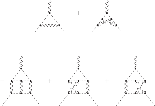
Figure 5: Graphs contributing to the vertex function which determines $\eta_{3}$ using the large $N$ conformal bootstrap method.

The original procedure to carry this out for the nonlinear $\sigma$ model in $d$-dimensions was given in [32] and involved extending the work of [33] which was specific to three dimensions. The first stage is to construct the consistency equations whose solution gives $\eta_{3}$. This has been given in [24, 25, 46] for the $O(N)$ Gross-Neveu model and that construction straightforwardly translates to the case of (2.5). The only major difference aside from the different labelling of the exponents is to append the factors deriving from the Pauli matrices in the vertex. Therefore we focus on outlining the formalism. The key ingredient is the vertex function which is denoted by $V(y,\alpha,\gamma;\delta,\delta^{\prime})$. Here $y$ is the same combination of amplitudes as before and the function depends on two regularizing parameters $\delta$ and $\delta^{\prime}$. These are required since in the derivation of the equation for $\eta$ given in [24, 25, 32, 46] there are divergent $2$-point functions. The divergences arise in the same context as those in the earlier $2$-point function analyses which required the introduction of the analytic regularization controlled by $\Delta$. As the conformal bootstrap also is a perturbative expansion in the vertex anomalous dimension the vertices of the graphs with conformal triangles also have to regularized. This is achieved by requiring that the external $\pi^{a}$ and one of the external $\psi^{i}$ legs of the graphs in Figure $5$ have their dimension shifted by $\delta$ and $\delta^{\prime}$ respectively, [24, 25, 46].

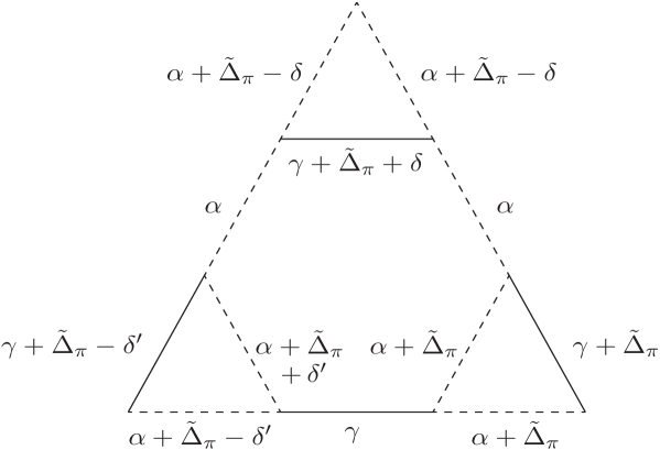
Figure 6: Regularized leading order graph for conformal bootstrap construction.

Having outlined features of the vertex function the formalism presented in [24, 25, 46] leads to the consistency equations. First the vertex function $V(y,\alpha,\gamma;\delta,\delta^{\prime})$ is defined by the sum of $\delta$-regularized graphs given in Figure $5$. The basic equation which in effect determines the hidden amplitide of the vertex order by order in large $N$ is

$$1~{}=~{}V(y,\alpha,\gamma;0,0)~{}.$$ (6.1)

In other words the sum of all the graphs is unity and it turns out that each graph is finite when evaluated after applying conformal techniques. Therefore the regularization for this was unnecessary, [24, 25, 46]. However, the graphs which contribute to the value of $\eta_{3}$ and equally to the lower order exponents are divergent which means the regularization cannot be neglected in their determination. Consequently the second consistency equation of the set is

$$\frac{2Nr(\alpha-1)}{3p(\gamma)} = \left.\frac{\left[1+2\chi_{\pi}\frac{\partial~{}}{\partial\delta^{\prime}}V(y,\alpha,\gamma;\delta,\delta^{\prime})\right]}{\left[1+2\chi_{\pi}\frac{\partial~{}}{\partial\delta}V(y,\alpha,\gamma;\delta,\delta^{\prime})\right]}\right|_{\delta=\delta^{\prime}=0}$$ (6.2)

where the same scaling functions as before are present. At leading order the right hand side is unity which means that the same value for $\eta_{1}$ is recovered as expected. At next order the one loop graph of Figure $5$ has to be included. However, it has to be evaluated with the regularized external vertices and conformal triangles. In order to illustrate the earlier points about the graphs in the large $N$ conformal bootstrap construction we have given the explicit allocation of exponents on the lines in Figure $6$ for the full graph corresponding to the one loop graph of Figure $5$. There for space considerations we have set

$$\chi_{\pi}~{}=~{}2\tilde{\Delta}_{\pi}~{}.$$ (6.3)

It is clear that there is a non-zero sum of the exponents at the top and bottom left vertices which are proportional to $\delta$ and $\delta^{\prime}$ respectively. Equally the sum of all the exponents at internal vertices are unique. The value of the graph in Figure $6$ has been determined in the context of the usual Gross-Neveu model as a function of the exponents of that model, [46]. So that formal expression can be adapted to this computation as the group factor is separate for the graph in Figure $6$. Exporting that function and inserting it into (6.1) and (6.2) we recover the earlier value of $\eta_{2}$ which provides a useful check on our conformal bootstrap construction.

The final stage is to include the remaining graphs of Figure $5$ in the two consistency equations. Again the values of the contributing integrals have been computed in [28] in the context of the usual Gross-Neveu model. So those master integral values need only be decorated with the group factors for the specific case we are interested in. Unlike the one loop graph of Figure $5$ some of the higher order $\delta$-regularized graphs cannot be evaluated completely. However for these cases it transpires that the difference

$$\left.\left[\frac{\partial~{}}{\partial\delta^{\prime}}V(y,\alpha,\gamma;\delta,\delta^{\prime})~{}-~{}\frac{\partial~{}}{\partial\delta}V(y,\alpha,\gamma;\delta,\delta^{\prime})\right]\right|_{\delta=\delta^{\prime}=0}$$ (6.4)

can be determined. This is all that is necessary since this difference for the higher order graphs is sufficient to deduce $\eta_{3}$ in the $1/N$ expansion of the right hand side of (6.2). If we denote the contributions to the right hand side of (6.2) from all the graphs in Figure $5$ except the one loop triangle by $V_{2}$ then

$$V_{2} = \left[\frac{\mu^{2}(14\mu^{2}-37\mu+28)}{18(\mu-1)^{3}}\Psi(\mu)~{}-~{}\frac{\mu^{2}(2\mu-5)(7\mu^{2}-18\mu+16)}{18(\mu-1)^{4}}\right.$$ (6.5)

$$\left.~{}-~{}\frac{\mu^{2}(\mu-16)}{36(\mu-1)^{2}}\Theta(\mu)~{}-~{}\frac{\mu^{2}}{6(\mu-1)}\Xi(\mu)\left[\Theta(\mu)+\frac{1}{(\mu-1)^{2}}\right]\right]\eta_{1}^{2}~{}.$$

This involves a new function $\Xi(\mu)$ which is related to a particular two loop graph introduced in [32] and denoted there by $I(\mu)$. In terms of $I(\mu)$ we have

$$I(\mu)~{}=~{}-~{}\frac{2}{3(\mu-1)}~{}+~{}\Xi(\mu)$$ (6.6)

so that the expansion of $\Xi(\mu)$ near two dimensions only involves multiple zeta values, [47]. For instance, the first few terms are

$$\Xi(1-\epsilon)~{}=~{}\frac{2}{3}\zeta_{3}\epsilon^{2}~{}+~{}\zeta_{4}\epsilon^{3}~{}+~{}\frac{13}{3}\zeta_{5}\epsilon^{4}~{}+~{}O(\epsilon^{5})~{}.$$ (6.7)

In three dimensions the integral $I(\mu)$ is known exactly, [32], since

$$I(\mbox{\small{$\frac{3}{2}$}})~{}=~{}2\ln 2~{}+~{}\frac{3\psi^{\prime\prime}(\mbox{\small{$\frac{1}{2}$}})}{2\pi^{2}}$$ (6.8)

which will be needed for our three dimensional estimates later. Finally including $V_{2}$ in (6.2) and expanding the one loop contribution from Figure $6$ to $O(1/N^{2})$ we find that

$$\eta_{3} = \left[\frac{(2\mu-3)}{18(\mu-1)^{2}}\left[\Phi(\mu)+3\Psi^{2}(\mu)\right]~{}-~{}\frac{[\mu^{3}+18\mu^{2}-21\mu+9]}{36(\mu-1)^{2}}\Theta(\mu)~{}-~{}\frac{\mu^{2}}{3(\mu-1)}\Theta(\mu)\Psi(\mu)\right.$$ (6.9)

$$\left.~{}-~{}\frac{\mu^{2}}{6(\mu-1)^{3}}\Xi(\mu)~{}-~{}\frac{[14\mu^{7}-15\mu^{6}-26\mu^{5}-77\mu^{4}+324\mu^{3}-297\mu^{2}+90\mu-9]}{18\mu^{2}(\mu-1)^{4}}\right.$$

$$\left.~{}-~{}\frac{[14\mu^{5}-37\mu^{4}-50\mu^{3}+228\mu^{2}-183\mu+27]}{18\mu(\mu-1)^{3}}\Psi(\mu)~{}-~{}\frac{\mu^{2}}{6(\mu-1)}\Xi(\mu)\Theta(\mu)\right]\eta_{1}^{3}$$

which completes the evaluation of all the critical exponents. To assist with analyses we have provided an attached data file where electronic versions of all the exponents computed here are given.

7 Results.

We devote this section to discussing our results and give estimates of critical exponents in three dimensions. As a first stage we must indicate that all the expressions derived here are consistent with known perturbation theory near four dimensions. Recently the three and four loop renormalization group functions have been provided for the chiral Heisenberg Gross-Neveu-Yukawa theory, [12, 14], which built on the early loop work of [10, 11]. Setting $d$ $=$ $4$ $-$ $2\epsilon$ in the $d$-dimensional exponents we find

$$\left.\frac{}{}\eta\right|_{d=4-2\epsilon} = \left[3\epsilon-\frac{9}{2}\epsilon^{2}-\frac{9}{4}\epsilon^{3}+\frac{3}{8}[16\zeta_{3}-3]\epsilon^{4}+\frac{9}{16}\left[16\zeta_{4}-16\zeta_{3}-1\right]\epsilon^{5}\right]\frac{1}{N}$$

$$+~{}\left[-~{}3\epsilon+\frac{99}{4}\epsilon^{2}-\frac{303}{8}\epsilon^{3}-\frac{3}{2}[16\zeta_{3}+13]\epsilon^{4}+3\left[49\zeta_{3}-12\zeta_{4}+3\right]\epsilon^{5}\right]\frac{1}{N^{2}}$$

$$+~{}\left[3\epsilon-\frac{153}{4}\epsilon^{2}+\left[72\zeta_{3}-\frac{51}{4}\right]\epsilon^{3}+\frac{3}{16}[576\zeta_{4}+3337-2104\zeta_{3}]\epsilon^{4}\right.$$

$$\left.~{}~{}~{}~{}+~{}\frac{3}{32}\left[1536\zeta_{5}-10645-6312\zeta_{4}+2104\zeta_{3}\right]\epsilon^{5}\right]\frac{1}{N^{3}}~{}+~{}O\left(\epsilon^{6};\frac{1}{N^{4}}\right)$$

$$\left.\frac{}{}\eta_{\phi}\right|_{d=4-2\epsilon} = 2\epsilon~{}+~{}\left[-2\epsilon+5\epsilon^{2}+\frac{1}{2}\epsilon^{3}+\left[-\frac{7}{4}-4\zeta_{3}\right]\epsilon^{4}+\frac{1}{8}\left[80\zeta_{3}-48\zeta_{4}-23\right]\epsilon^{5}\right]\frac{1}{N}$$

$$+~{}\left[2\epsilon+\frac{69}{2}\epsilon^{2}+\left[48\zeta_{3}-\frac{625}{4}\right]\epsilon^{3}+\left[155-128\zeta_{3}+72\zeta_{4}\right]\epsilon^{4}\right.$$

$$\left.~{}~{}~{}~{}+~{}2\left[73\zeta_{3}-96\zeta_{4}+48\zeta_{5}+18\right]\epsilon^{5}\right]\frac{1}{N^{2}}~{}+~{}O\left(\epsilon^{6};\frac{1}{N^{3}}\right)$$

$$\left.\frac{1}{\nu}\right|_{d=4-2\epsilon} = 2~{}-~{}2\epsilon$$ (7.1)

$$+~{}\left[-18\epsilon+39\epsilon^{2}-\frac{9}{2}\epsilon^{3}+\left[-\frac{9}{4}-36\zeta_{3}\right]\epsilon^{4}~{}+~{}\frac{3}{8}\left[208\zeta_{3}-144\zeta_{4}-3\right]\epsilon^{5}\right]\frac{1}{N}$$

$$+~{}\left[438\epsilon-\frac{3005}{2}\epsilon^{2}+\left[\frac{3721}{4}-552\zeta_{3}\right]\epsilon^{3}+\left[744+3608\zeta_{3}-828\zeta_{4}+1360\zeta_{5}\right]\epsilon^{4}\right.$$

$$\left.~{}~{}~{}~{}+~{}\frac{1}{2}\left[1760\zeta_{3}^{2}-16532\zeta_{3}+10824\zeta_{4}-17728\zeta_{5}+6800\zeta_{6}-365\right]\epsilon^{5}\right]\frac{1}{N^{2}}$$

$$+~{}O\left(\epsilon^{6};\frac{1}{N^{3}}\right)~{}.$$

Comparing with the results of [10, 12, 13, 14] and allowing for the different $\epsilon$ expansion convention we find exact agreement with the exponents of [10, 12, 13, 14]. For future five loop computations we have also given the $O(\epsilon^{5})$ terms. We have also checked that the $\epsilon$ expansion of $\omega_{1}$ near four dimensions is in agreement with one of the eigen-critical exponents of the Hessian defined by the derivatives of the two $\beta$-functions of [14]. This check is similar to that carried out in the Ising Gross-Neveu model [43]. For similar reasons we give the $\epsilon$ expansion of the exponents in $d$ $=$ $2$ $-$ $2\epsilon$ to the same order. We have

$$\left.\frac{}{}\eta\right|_{d=2-2\epsilon} = \left[3\epsilon^{2}+3\epsilon^{3}+3\epsilon^{4}+\left[3+6\zeta_{3}\right]\epsilon^{5}\right]\frac{1}{N}$$

$$+~{}\left[-~{}\frac{9}{2}\epsilon^{2}-\frac{45}{2}\epsilon^{3}-36\epsilon^{4}+\left[-30\zeta_{3}-45\right]\epsilon^{5}\right]\frac{1}{N^{2}}$$

$$+~{}\left[-~{}9\epsilon^{2}+24\epsilon^{3}+159\epsilon^{4}+\left[396-\frac{111}{2}\zeta_{3}\right]\epsilon^{5}\right]\frac{1}{N^{3}}~{}+~{}O\left(\epsilon^{6};\frac{1}{N^{4}}\right)$$

$$\left.\frac{}{}\eta_{\phi}\right|_{d=2-2\epsilon} = 2~{}+~{}2\epsilon~{}+~{}\left[-2\epsilon-6\epsilon^{2}-6\epsilon^{3}+\left[-6-4\zeta_{3}\right]\epsilon^{4}+\left[-~{}12\zeta_{3}-6\zeta_{4}-6\right]\epsilon^{5}\right]\frac{1}{N}$$

$$+~{}\left[-~{}10\epsilon-3\epsilon^{2}+23\epsilon^{3}+\left[78-44\zeta_{3}\right]\epsilon^{4}+\left[36\zeta_{3}-66\zeta_{4}+96\right]\epsilon^{5}\right]\frac{1}{N^{2}}$$

$$+~{}O\left(\epsilon^{6};\frac{1}{N^{3}}\right)$$

$$\left.\frac{}{}\frac{1}{\nu}\right|_{d=2-2\epsilon} = -~{}2\epsilon~{}+~{}\left[-~{}6\epsilon^{2}+6\epsilon^{3}+6\epsilon^{4}+\left[6-12\zeta_{3}\right]\epsilon^{5}\right]\frac{1}{N}$$ (7.2)

$$+~{}\left[8\epsilon^{2}+9\epsilon^{3}+\left[67+90\zeta_{3}\right]\epsilon^{4}+\left[240\zeta_{3}+135\zeta_{4}-178\right]\epsilon^{5}\right]\frac{1}{N^{2}}$$

$$+~{}O\left(\epsilon^{6};\frac{1}{N^{3}}\right)~{}.$$

Having established the consistency of our $d$-dimensional critical exponents with known four dimensional perturbation theory it is a simple exercise to determine the values in three dimensions. We have

$$\left.\frac{}{}\eta\right|_{d=3} = \frac{4}{\pi^{2}N}~{}+~{}\frac{64}{3\pi^{4}N^{2}}~{}+~{}\frac{8[378\zeta_{3}-36\pi^{2}\ln(2)-45\pi^{2}-332]}{9\pi^{6}N^{3}}~{}+~{}O\left(\frac{1}{N^{4}}\right)$$

$$\left.\frac{}{}\eta_{\phi}\right|_{d=3} = 1~{}+~{}\frac{16[3\pi^{2}+16]}{3\pi^{4}N^{2}}~{}+~{}O\left(\frac{1}{N^{3}}\right)$$

$$\left.\frac{1}{\nu}\right|_{d=3} = 1~{}-~{}\frac{16}{\pi^{2}N}~{}+~{}\frac{[144\pi^{2}+1664]}{3\pi^{4}N^{2}}~{}+~{}O\left(\frac{1}{N^{3}}\right)$$ (7.3)

where the $O(1/N)$ correction to $\eta_{\phi}$ is zero or

$$\left.\frac{}{}\eta\right|_{d=3} = \frac{0.4052845}{N}~{}+~{}\frac{0.219008}{N^{2}}~{}-~{}\frac{0.525197}{N^{3}}~{}+~{}O\left(\frac{1}{N^{4}}\right)$$

$$\left.\frac{}{}\eta_{\phi}\right|_{d=3} = 1~{}+~{}\frac{2.497169}{N^{2}}~{}+~{}O\left(\frac{1}{N^{3}}\right)$$

$$\left.\frac{1}{\nu}\right|_{d=3} = 1~{}-~{}\frac{1.621139}{N}~{}+~{}\frac{10.557615}{N^{2}}~{}+~{}O\left(\frac{1}{N^{3}}\right)$$ (7.4)

numerically.

	$1/\nu$	$\eta_{\phi}$	$\eta$	$\nu$
$\epsilon$ expansion $[2,2]$ Padé [14]	$0.6426$	$0.9985$	$0.1833$	$-$
$\epsilon$ expansion $[3,1]$ Padé [14]	$0.6447$	$0.9563$	$0.1560$	$1.2352$
Functional RG [48]	$0.795$	$1.032$	$0.071$	$1.26$
Monte Carlo [49]	$(0.98)$		$0.20(2)$	$1.02(1)$
Monte Carlo [50]	$(1.19)$	$0.70(15)$		$0.84(4)$
Large $N$	$0.8458$	$1.1849$	$0.1051$	$1.1823$

Table $1$. Comparison of large $N$ Padé estimates with other methods for $N$ $=$ $4$ for the chiral Heisenberg Gross-Neveu model.

Equipped with these three dimensional expressions we can now provide estimates for the exponents in the case which is of interest to graphene problems. Therefore recalling our convention for the spinor trace (2.2) the value of $N$ we use in order to compare with the numerical estimates of critical exponents of other methods for (2.5) is $N$ $=$ $4$. Given this we have determined numerical estimates for the three critical exponents using Padé approximants. These are given in the last line of Table $1$ together with results quoted in [14] by other approaches for comparison. In the table bracketed values for $1/\nu$ represent the value derived from $\nu$ which was computed directly. For the large $N$ estimates we have quoted the $[1,2]$, $[0,2]$ and $[1,1]$ Padé approximants for $\eta$, $\eta_{\phi}$ and $1/\nu$ respectively. In general the values for large $N$ are similar but larger than those of the functional renormalization group values of [48] for $\eta_{\phi}$ and $1/\nu$. For $\eta$ the situation is much different with virtually no overlap for any of the different analyses. As [14] also considered the XY Gross-Neveu model we have also provided the parallel results for $N$ $=$ $4$ in Table $2$ in order to compare results for the same methods in a different context. Again it is the case that the estimates for $\eta_{\phi}$ and $1/\nu$ are slightly larger than those of the functional renormalization group values in [14] with again no clear consensus for $\eta$. Although it is worth noting that the large $N$ estimate for $\eta$ is a $[1,1]$ Padé since the value of $\eta_{3}$ for that model has not been computed.

	$1/\nu$	$\eta_{\phi}$	$\eta$
$\epsilon$ expansion $[2,2]$ Padé [14]	$0.840$	$0.810$	$0.117$
$\epsilon$ expansion $[3,1]$ Padé [14]	$0.841$	$0.788$	$0.108$
Functional RG [51]	$0.862$	$0.88$	$0.062$
Monte Carlo [52]	$1.06(5)$	$0.71(3)$
Large $N$	$0.9026$	$0.9023$	$0.0872$

Table $2$. Comparison of large $N$ Padé estimates with other methods for $N$ $=$ $4$ for the chiral XY Gross-Neveu model.

Perhaps a more instructive way of viewing the situation with the exponent estimates is to use a graphical representation motivated by the functional renormalization group approach [9]. One aspect of that method is that it is not limited to a discrete spacetime dimension. In other words the critical exponents can be determined as functions of $d$ and plots of the three exponents in $2$ $<$ $d$ $<$ $4$ were given in [9]. As our expansion parameter, $1/N$, is dimensionless in $d$-dimensions it is possible to provide similar plots for the same exponents. By this we mean that we can plot the various Padé approximants used to obtain the estimates in Table $1$ for the chiral Heisenberg Gross-Neveu model as functions of $d$. These are given in Figure $7$ for $N$ $=$ $4$ except that the $[1,1]$ Padé is used for $\eta$. This is because we do not have a closed analytic form for the $\Xi(\mu)$ as a function of $\mu$. Instead we have used the first two terms of $\eta$. However in the plot of $\eta$ we have included the $[2,1]$ Padé estimate, indicated by an open circle, and the $[1,2]$ estimate indicated by a solid circle. These are meant to guide roughly where the $d$-dimensional line would intersect if $\eta_{3}$ was known as an analytic function in $d$-dimensions. One interesting aspect of the three curves in Figure $7$ is that they are in good qualitative agreement with those of the right hand panels of Figures $1$, $2$ and $3$ of [9]. By this we mean that the shape in terms of concavity and convexity for $\eta_{\phi}$ and $1/\nu$ are very similar as well as the offset of the peak for $\eta$ which is not in the neighbourhood of $d$ $=$ $3$. Finally, in order to assist this comparison we have included similar plots for the XY Gross-Neveu model when $N$ $=$ $4$ and the ordinary or Ising Gross-Neveu model for $N$ $=$ $8$ in Figures $8$ and $9$ respectively. The latter value of $N$ in that case is the parallel one to compare with [9]. In Figure $8$ only the first two terms of $\eta$ were available which why the Padé estimate lies on the line. While the shapes of the plots for the Ising Gross-Neveu model are also qualitatively similar to those of [9] it is worth noting that the one for $\eta_{\phi}$ differs in concavity to that for the chiral Heisenberg Gross-Neveu model which is consistent with the functional renormalization group approach.

Figure 7: Dependence of Padé approximants to critical exponents $\eta$, $\eta_{\phi}$ and $1/\nu$ for the chiral Heisenberg Gross-Neveu model when $N$ $=$ $4$. In the $\eta$ plot the open circle is the $[2,1]$ Padé approximant using $\eta$ at $O(1/N^{3})$ and the solid circle is the $[1,2]$ Padé approximant.

Figure 8: Dependence of Padé approximants to critical exponents $\eta$, $\eta_{\phi}$ and $1/\nu$ for the Gross-Neveu XY model when $N$ $=$ $4$.

Figure 9: Dependence of Padé approximants to critical exponents $\eta$, $\eta_{\phi}$ and $1/\nu$ for the Ising Gross-Neveu model when $N$ $=$ $8$.

8 Discussion.

We have completed the evaluation of the three core critical exponents $\eta$, $\eta_{\phi}$ and $1/\nu$ to several orders in the large $N$ expansion as a function of the spacetime dimension $d$ for the chiral Heisenberg Gross-Neveu universality class. The $\epsilon$ expansion of the expressions near four dimensions agrees exactly with the recent explicit four loop renormalization group functions of (2.4) at the Wilson-Fisher fixed point, given in [14]. Indeed our large $N$ results are an important independent check on that work. Moreover we have provided the next terms in the series as a future check for any five loop renormalization of (2.4). As the exponents depend on $d$, plots of the Padé approximant of each exponent in dimensions $2$ $<$ $d$ $<$ $4$ have been given in order to compare with the functional renormalization group approach of [9] where a sharp regulator was used. All the large $N$ plots for not only the chiral Heisenberg Gross-Neveu universality class but the Ising and XY Gross-Neveu classes in $d$-dimensions are in good qualitative agreement with [9]. Again this consistency provides independent evidence that these methods are capturing the proper and general behaviour of the exponents of the universality class across the dimensions. At the outset we drew attention to Figures $1$, $2$ and $3$ of [9] in relation to the status of results available for the Ising and chiral Heisenberg Gross-Neveu universality classes. In addition to the three and four loop results of [12, 13, 14] the results here are now edging towards the latter class having commensurate data with the former. What is lacking is Monte Carlo results and higher order two dimensional perturbative renormalization group functions. The latter should be possible to obtain to four loops with the recent derivation of the $\beta$-function for the Ising Gross-Neveu model in two dimensions, [15]. This is not as straightforward a computation as that for the four dimensional case, [12, 13, 14]. In two dimensions quartic fermion self-interactions are not multiplicatively renormalizable when the Lagrangian is dimensionally regularized. Instead additional evanescent quartic interactions are generated and their presence means that one has to be careful in extracting the true renormalization group functions after the regularization is lifted. Aside from this technical issue it should be possible in the future to add this extra information to the analysis of the chiral Heisenberg universality class.

Acknowledgements. The author thanks Prof I.F. Herbut, Dr L. Mihaila, Dr M. Scherer, R.M. Simms and Prof S.J. Hands for valuable discussions. The work was carried out with the support in part of the STFC through the Consolidated Grant ST/L000431/1. The graphs were drawn with the Axodraw package [53]. Computations were carried out in part using the symbolic manipulation language Form, [54, 55].

- [1] D. Gross & A. Neveu, Phys. Rev. D10 (1974), 3235.
- [2] J. Ashkin & E. Teller, Phys. Rev. 64 (1943), 178.
- [3] T.O. Wehling, E. Şaşıoğlu, C. Friedrich, A.I. Lichtenstein, M.I. Katsnelson & S. Blügel, Phys. Rev. Lett. 106 (2011), 236805.
- [4] M.V. Ulybyshev, P.V. Buividovich, M.I. Katsnelson & M.I. Polikarpov, Phys. Rev. Lett. 111 (2013), 056801.
- [5] I.F. Herbut, Phys. Rev. Lett. 97 (2006), 146401.
- [6] I.F. Herbut, V. Juric̆ić & O. Vafek, Phys. Rev. B80 (2009), 075432.
- [7] S. Sorella, Y. Otsuka & S. Yunoki, Sci. Rep. 2 (2012), 992.
- [8] F.F. Assaad & I.F. Herbut, Phys. Rev. X3 (2013), 031010.
- [9] L. Janssen & I.F. Herbut, Phys. Rev. B89 (2014), 205403.
- [10] B. Rosenstein, H.-L. Yu & A. Kovner, Phys. Lett. B314 (1994), 381.
- [11] L. Kärkkäinen, R. Lacaze, P. Lacock & B. Petersson, Nucl. Phys. B415 (1994), 781.
- [12] L.N. Mihaila, N. Zerf, B. Ihrig, I.F. Herbut & M.M. Scherer, Phys. Rev. B96 (2017), 165133.
- [13] L. Fei, S. Giombi, I.R. Klebanov & G. Tarnopolsky, Prog. Theor. Exp. Phys. (2016), 12C105.
- [14] N. Zerf, L.N. Mihaila, P. Marquard, I.F. Herbut & M.M. Scherer, Phys. Rev. D96 (2017), 096010.
- [15] J.A. Gracey, T. Luthe & Y. Schröder, Phys. Rev. D94 (2016), 125028.
- [16] W. Wetzel, Phys. Lett. B153 (1985), 297.
- [17] A.W.W. Ludwig, Nucl. Phys. B285 (1987), 97.
- [18] J.A. Gracey, Nucl. Phys. B341 (1990), 403.
- [19] J.A. Gracey, Nucl. Phys. B367 (1991), 657.
- [20] C. Luperini & P. Rossi, Ann. Phys. 212 (1991), 371.
- [21] J.A. Gracey, Nucl. Phys. B802 (2008), 330.
- [22] J.A. Gracey, Int. J. Mod. Phys. A6 (1991), 395, 2755(E).
- [23] J.A. Gracey, Phys. Lett. B297 (1992), 293.
- [24] S.É. Derkachov, N.A. Kivel, A.S. Stepanenko & A.N. Vasil’ev, hep-th/9302034.
- [25] A.N. Vasil’ev, S.É. Derkachov, N.A. Kivel & A.S. Stepanenko, Theor. Math. Phys. 94 (1993), 127.
- [26] A.N. Vasil’ev & A.S. Stepanenko, Theor. Math. Phys. 97 (1993), 1349.
- [27] J.A. Gracey, Int. J. Mod. Phys. A9 (1994), 567.
- [28] J.A. Gracey, Int. J. Mod. Phys. A9 (1994), 727.
- [29] J. Zinn-Justin, Nucl. Phys. B367 (1991), 105.
- [30] A.N. Vasil’ev, Y.M. Pismak & J.R. Honkonen, Theor. Math. Phys. 46 (1981), 104.
- [31] A.N. Vasil’ev, Y.M. Pismak & J.R. Honkonen, Theor. Math. Phys. 47 (1981), 465.
- [32] A.N. Vasil’ev, Y.M. Pismak & J.R. Honkonen, Theor. Math. Phys. 50 (1982), 127.
- [33] G. Parisi, Lett. Nuovo Cim. 4 (1971), 777.
- [34] F.A. Dolan & H. Osborn, Nucl. Phys. B599 (2001), 459.
- [35] R. Rattazzi, V.S. Rychkov & E. Tonni, JHEP 0812 (2008), 031.
- [36] S. El-Showk, M.F. Paulos, D. Poland, S. Rychkov, D. Simmons-Duffin & A. Vichi, Phys. Rev. D86 (2012), 025022.
- [37] F. Kos, D. Poland & D. Simmons-Duffin, JHEP 1406 (2014), 091.
- [38] S.-S. Lee, Phys. Rev. B76 (2007), 075103.
- [39] B. Roy, V. Juric̆ić & I.F. Herbut, Phys. Rev. B87 (2013), 041401(R).
- [40] A. Hasenfratz & P. Hasenfratz, Phys. Lett. B297 (1992), 166.
- [41] A.N. Vasil’ev & M.Yu. Nalimov, Theor. Math. Phys. 55 (1983), 423.
- [42] A.N. Vasil’ev & M.Yu. Nalimov, Theor. Math. Phys. 56 (1983), 643.
- [43] J.A. Gracey, Phys. Rev. D96 (2017), 065015.
- [44] A.N. Manashov & M. Strohmaier, arXiv:1711.02493 [hep-th].
- [45] M. d’Eramo, L. Peliti & G. Parisi, Lett. Nuovo Cim. 2 (1971), 878.
- [46] J.A. Gracey, Z. Phys. C59 (1993), 243.
- [47] I. Bierenbaum, & S. Weinzierl, Eur. Phys. J. C32 (2003), 67.
- [48] B. Knorr, Phys. Rev. B97 (2018), 075129.
- [49] Y. Otsuka, S. Yunoki & S. Sorella, Phys. Rev. X6 (2016), 011029.
- [50] F. Parisen Toldin, M. Hohenadler, F.F. Assaad & I.F. Herbut, Phys. Rev. B91 (2015), 165108.
- [51] L. Classen, I.F. Herbut & M.M. Scherer, Phys. Rev. B96 (2017), 115132.
- [52] Z.-X. Li, Y.-F. Jiang, S.-K. Jian & H. Yao, Nature Communications 8 (2017), 314.
- [53] J.C. Collins & J.A.M. Vermaseren, arXiv:1606.01177 [cs.OH].
- [54] J.A.M. Vermaseren, math-ph/0010025.
- [55] M. Tentyukov & J.A.M. Vermaseren, Comput. Phys. Commun. 181 (2010), 1419.