Simple waves in a two-component Bose-Einstein condensate

Abstract

We consider dynamics of simple waves in a two-component Bose-Einstein condensates. The evolution of the condensate is described by the Gross-Pitaevskii equations which can be reduced for simple wave solutions to a system of ordinary differential equations which coincide with those derived by Ovsyannikov for the two-layer fluid dynamics. We solve the Ovsyannikov system for two typical situations of large and small difference between inter-species and intra-species nonlinear interaction constants. Our analytic results are confirmed by numerical simulations.

,

Keywords: multicomponent Bose-Einstein condensates, simple waves, Riemann problem, dispersive shock waves, solitons, solitary waves, wave breaking, Whitham modulation equations

1 Introduction

The study of multi-component nonlinear waves is one of the fascinating topics which has potential applications to dynamics of Bose-Einstein condensates (BECs) [1] and of optical pulses in fibers [2]. The dynamics of such a condensate is much more complicated compared with the one-component case. In particular, two types of motions are possible in two-component BECs—“density wave” with in-phase motion of the components and “polarization waves” with counter-phase their motion. It has been noticed [3] that the polarization dynamics can be separated from the density dynamics even for the case of large amplitude waves, if the difference between intra- and inter-species interaction constants is small. In this case, the structures arising during the evolution of two-component condensate were studied in [4] under the assumption that the total density is preserved what is a good approximation in this case. In this paper, we go beyond this approximation and study the dynamics without imposing any restrictions on the nonlinear interaction constants except that we assume that the components can mix in the same volume of a trap. To study typical situations, we derive differential equations describing the evolution of density and flow velocity of the condensate components for the case of the so-called “simple wave solutions” when all physical variables depend on the single parameter. This class of solutions can be applied to the problem of the evolution of an initial discontinuity for two characteristic cases. It will be shown that when the parameters of the condensate are close to the miscibility boundary, the total density remains practically constant with very good accuracy. For the situation of weak interaction of the condensate component, we find that compound simple waves can be formed that consist of merged one-component and two-component rarefaction waves. Approximate solutions are found and their accuracy is confirmed by numerical simulations.

2 The model

One-dimensional dynamics of a two-component Bose-Einstein condensate without the external potential is described with a high accuracy by the system of the Gross-Pitaevskii (GP) equations which can be written in non-dimensional form as

$${\rm i}\frac{\partial\psi_{i}}{\partial t}=-\frac{1}{2}\frac{\partial^{2}\psi_{i}}{\partial x^{2}}+g_{ii}|\psi_{i}|^{2}\psi_{i}+g_{ij}|\psi_{j}|^{2}\psi_{i},$$ (1)

where $i,j=1,2~{}(i\neq j)$ label the corresponding condensate components, $(\psi_{1},\psi_{2})$ are the wave functions of the components which are normalized to the number of particles,

$$\int|\psi_{i}|^{2}dx=N_{i},$$

so that $|\psi_{i}|^{2}=\rho_{i}$ is the density of particles in the $i$-th component. The gradient of the phase $\varphi_{i}$ of the wave function $\psi_{i}=\sqrt{\rho_{i}}\exp({\rm i}\varphi_{i})$ is equal to the flow velocity $u_{i}$ of $i$-th component. Parameters $g_{ii}$ are the constants of interaction between atoms of component $i$, and $g_{ij}$ are the constants of interaction between atoms of different species. Usually $g_{12}=g_{21}$, what we will assume in what follows.

If the phase $\varphi_{i}$ is a single-valued function of coordinates, what means physically that there are no vortices in the condensate, the wave functions of the two-component condensate can be represented as

$$\psi_{i}=\sqrt{\rho_{i}(x,t)}\exp\left({\rm i}\int^{x}u_{i}(x^{\prime},t)dx^{\prime}-{\rm i}{\mu_{i}}t\right),$$ (2)

where $\mu_{i}$ is the chemical potential of the $i$-th component (see [5]). Substitution of (2) into (1) and separation of real and imaginary parts followed by differentiation of one of the equations with respect to $x$ cast the GP equations to the so-called “hydrodynamic form”:

$$\eqalign{{\partial_{t}\rho_{i}}+{\partial_{x}}(\rho_{i}u_{i})=0,\cr{\partial_{t}u_{i}}+u_{i}{\partial_{x}u_{i}}+g_{ii}{\partial_{x}\rho_{i}}+g_{ij}{\partial_{x}\rho_{j}}\cr\qquad+{\partial_{x}}\left(\frac{({\partial_{x}}\rho_{i})^{2}}{8\rho_{i}^{2}}-\frac{{\partial_{x}^{2}}\rho_{i}}{4\rho_{i}}\right)=0.}$$ (3)

The first equation (3) provides conservation of the number of particles in the corresponding condensate component. If we drop out the last dispersion term in the second equation (3), then we get the Euler two-fluid hydrodynamics equations,

$$\eqalign{{\partial_{t}\rho_{i}}+{\partial_{x}}(\rho_{i}u_{i})=0,\cr{\partial_{t}u_{i}}+u_{i}{\partial_{x}u_{i}}+g_{ii}{\partial_{x}\rho_{i}}+g_{ij}{\partial_{x}\rho_{j}}=0.}$$ (4)

This system describes dynamics of condensates at characteristic scales much greater than the healing length equal to unity in our non-dimensional variables.

3 Simple waves

In simple wave solutions the variables $\rho_{i}$, $u_{i}$ are assumed to depend on the space and time coordinated via single function and it is convenient to choose the characteristic velocity $c=c(x,t)$ as such a function. Obviously, $c$ is a local velocity of the mode under consideration and therefore it satisfies the equation

$$\partial_{t}c+c\,\partial_{x}c=0.$$ (5)

It it easy to find that the characteristic equation for the system (4) can be written in the form

$$(1-v_{1}^{2})(1-v_{2}^{2})=\frac{g_{12}^{2}}{g_{11}g_{22}},$$ (6)

where, to simplify the notation, we have introduced the variables $v_{1}$ and $v_{2}$ according to

$$u_{1}-c=v_{1}\sqrt{g_{11}\rho_{1}},\qquad u_{2}-c=v_{2}\sqrt{g_{22}\rho_{2}}.$$ (7)

In the case when $g_{12}^{2}<g_{11}g_{22}$, what means physically that the components of the condensate are miscible (see [6]), the left part of the characteristic equation (6) is less than unity. As was mentioned in Introduction, we confine ourselves to this situation only.

Since the variables $\rho_{i}$ and $u_{i}$ depend on the characteristic velocity $c$ only, the equations (4) reduce to the system of ordinary differential equations

$$\eqalign{\rho_{i}u_{i}^{\prime}+(u_{i}-c)\rho_{i}^{\prime}=0,\cr(u_{i}-c)u_{i}^{\prime}+g_{ii}\rho_{i}^{\prime}+g_{ij}\rho_{j}^{\prime}=0,}$$ (8)

where the prime denotes the derivative with respect to $c$ ($\rho_{i}^{\prime}=d\rho_{i}/dc$ and $u_{i}^{\prime}=du_{i}/dc$). In terms of variables $v_{i}$ this system reads

$$\eqalign{\rho_{i}v_{i}^{\prime}+\frac{3}{2}v_{i}\rho_{i}^{\prime}+\sqrt{\frac{\rho_{i}}{g_{ii}}}=0,\cr v_{i}\rho_{i}v_{i}^{\prime}+\left(1+\frac{v_{i}^{2}}{2}\right)\rho_{i}^{\prime}+\frac{g_{ij}}{g_{ii}}\rho_{j}^{\prime}+\sqrt{\frac{\rho_{i}}{g_{ii}}}v_{i}=0.}$$ (9)

Solving it with respect to derivatives, we arrive at the system

$$\eqalign{\frac{d\rho_{1}}{dc}=-\frac{2}{3}\sqrt{g_{22}(1-v_{2}^{2})}\,f,\cr\frac{dv_{1}}{dc}=\frac{v_{1}}{\rho_{1}}\sqrt{g_{22}(1-v_{2}^{2})}\,f-\frac{1}{\sqrt{g_{11}\rho_{1}}},\cr\frac{d\rho_{2}}{dc}=\frac{2}{3}\sqrt{g_{11}(1-v_{1}^{2})}\,f,\cr\frac{dv_{2}}{dc}=-\frac{v_{2}}{\rho_{2}}\sqrt{g_{11}(1-v_{1}^{2})}\,f-\frac{1}{\sqrt{g_{22}\rho_{2}}},}$$ (10)

where

$$\eqalign{f(\rho_{1},\rho_{2},v_{1},v_{2})\cr\;\;=\frac{\sqrt{g_{22}\rho_{1}}\rho_{2}v_{1}(1-v_{2}^{2})+\sqrt{g_{11}\rho_{2}}\rho_{1}v_{2}(1-v_{1}^{2})}{\sqrt{g_{11}}g_{22}\rho_{2}v_{1}^{2}(1-v_{2}^{2})^{3/2}-\sqrt{g_{22}}g_{11}\rho_{1}v_{2}^{2}(1-v_{1}^{2})^{3/2}}.}$$ (11)

We call these equations as Ovsyannikov equations since similar equations were first obtained by him in the theory of two-layer shallow water dynamics [7]. These equations should be solved with the initial conditions

$$\eqalign{\rho_{1}|_{t=0}=\rho_{10},\qquad v_{1}|_{t=0}=v_{10},\cr\rho_{2}|_{t=0}=\rho_{20},\qquad v_{2}|_{t=0}=v_{20}.}$$ (12)

Typically, $v_{10}$ and $v_{20}$ can be found numerically by solving the algebraic system which consists of the characteristic equation (6) and the conditions $c|_{t=0}\equiv c_{0}=u_{10}-v_{10}\sqrt{g_{11}\rho_{10}}=u_{20}-v_{20}\sqrt{g_{22}\rho_{20}}$, where we have defined initial velocities as $u_{1}|_{t=0}\equiv u_{10}$ and $u_{2}|_{t=0}\equiv u_{20}$. In important particular case when the initial flow velocities are equal to zero ($u_{10}=u_{20}=0$), the parameters $v_{10}$ and $v_{20}$ are given analytically by simple formulas

$$\eqalign{v_{10}^{2}=\frac{g_{11}\rho_{10}+g_{22}\rho_{20}\pm\sqrt{\Delta}}{2g_{11}\rho_{10}},\cr v_{20}^{2}=\frac{g_{11}\rho_{10}+g_{22}\rho_{20}\pm\sqrt{\Delta}}{2g_{22}\rho_{20}},}$$ (13)

where $\Delta=(g_{11}\rho_{10}-g_{22}\rho_{20})^{2}+4g_{12}^{2}\rho_{10}\rho_{20}$. Here the upper sign ($+$) corresponds to the in-phase motion of the components associated mainly with the total density oscillations, and the lower sign ($-$) corresponds to out-of-phase motion of the components associated mainly with relative motion of the components in the “polarization” mode. The system of the Ovsyannikov equations (10) can be easily solved numerically. Below we apply it to the problem of evolution of an initial discontinuity in the flow data, that is to the so-called Riemann problem.

4 Solution of the Riemann problem

We apply here the above developed theory to description of wave structures evolving from initial discontinuities. Let the initial conditions have a step-like form

$$\eqalign{\rho_{1}|_{t=0}=\cases{\rho_{1}^{L},&for $x<0$\\ \rho_{1}^{R},&for $x>0$\\ },\cr\rho_{2}|_{t=0}=\cases{\rho_{2}^{L},&for $x<0$\\ \rho_{2}^{R},&for $x>0$\\ }.}$$ (14)

We assume that the initial flow velocities are equal to zero ($u_{10}=u_{20}=0$), i.e. the components are at rest at $t=0$, and that the density of the second component at the left boundary is equal to zero, too ($\rho_{2}^{L}=0$). This means that we have a ‘vacuum’ of the component $\rho_{2}$ for $x<0$ at the initial moment of time. The dependence on the spatial coordinate and the time in this problem is self-similar, $c=x/t$, since our initial conditions contain no parameters with the dimensions of length. For brevity we denote $g_{11}=g_{22}=g$ and $g_{12}=\widetilde{g}$. We consider two typical situations: the case when the interaction between the components differs little from the interaction of particles which belong to the same component ($g-\widetilde{g}\ll g$), and when the intra-components and inter-components interactions are very different ($\widetilde{g}\ll g$).

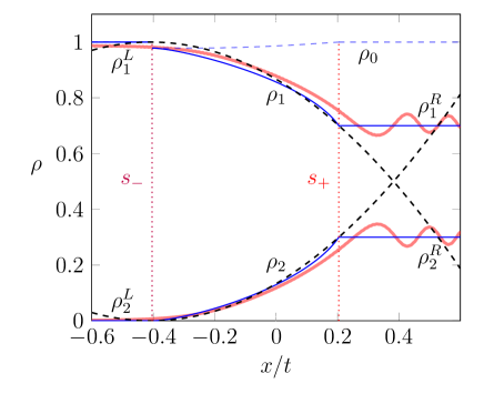
Figure 1: In this plot we compare the numerical simulations for the density field $\rho(c=x/t)$ of the GP equations (1) (red lines) with the numerical solution of the Ovsyannikov equations (10) (blue lines) and the approximation (17) (black dashed lines). The vertical dotted lines indicate velocities of the edges. The initial profile is characterized by $\rho_{1}^{L}=1$, $\rho_{2}^{L}=0$, $\rho_{1}^{R}=0.7$, $\rho_{2}^{R}=0.3$ and the interaction constants are equal to $g_{11}=g_{22}=g=1$, $g_{12}=\widetilde{g}=0.9$. The numerical solution of the Ovsyannikov equations confirms the approximate constancy of the total density $\rho_{0}$ (blue dashed line) in the polarization mode.

4.1 Numerical solution of the Ovsyannikov equations

First of all, we consider the case when $g-\widetilde{g}\ll g$. This regime is of considerable practical interest. For instance, it is realized in the condensate of ⁸⁷Rb atoms in different states of the hyperfine structure ($|1,-1\rangle$ and $|2,-2\rangle$) (see, e.g., [8]). If $g-\widetilde{g}\ll g$, then the numerical solution yields the distributions shown in figure 1 by red lines. Here in each component the rarefaction waves are formed. These are simple waves in the polarization mode since they do not practically affect the total density of the condensate. In this flow one component replaces the another one leaving the total density practically constant, $\rho_{0}=\rho_{1}^{L}+\rho_{2}^{L}=\rho_{1}^{R}+\rho_{2}^{R}$, as one can see in the numerical solution of the Ovsyannikov equations (10) shown in the figure 1 by a blue dashed line. This property of the polarization mode in this regime was indicated in [3, 9] and our numerics serves as its additional justification.

Edges of the rarefaction wave propagate with velocities

$$s_{-}=-\sqrt{\frac{8(g-\widetilde{g})\rho_{1}^{R}\rho_{2}^{R}}{\rho_{0}}},\quad s_{+}=\sqrt{\frac{2(g-\widetilde{g})\rho_{1}^{R}\rho_{2}^{R}}{\rho_{0}}}.$$ (15)

It is easy to see that in the limit $\widetilde{g}/g\rightarrow 1$ the velocities of the left and the right edges tend to zero. In figure 1 we illustrate such a structure and compare the numerical solution of the GP equations (1) with the numerical solution of the Ovsyannikov equations (10). Black dashed lines correspond to the approximate analytical solution of the Ovsyannikov equations for the case when the density of one of the components is much greater than the density of the other component. This analytical solution will be obtained below.

In the other case, when $\widetilde{g}\ll g$, we obtain distributions shown in figure 2. Here interaction between the components is weak. In this solution, the second component flows with formation of the rarefaction wave similar to that for a one-component condensate flowing into vacuum. The density of particles in this wave vanishes at the point $x=s_{-}t$, where the velocity of the left edge is equal to $s_{-}=v_{20}\sqrt{g\rho_{1}^{L}}$. Density of the first component at the left edge of the simple wave is determined numerically from the continuity condition $\rho_{1}^{L}=\rho_{1}(s_{-})$. In the limit $\tilde{g}/g\rightarrow 0$, the density of the first component remains constant along a single rarefaction wave. One can say that in this case the second component with a non-zero density at the right side of the discontinuity flows into the first one, only slightly perturbing it in the flow region. In figure 2 we compare the numerical solution of the GP equations (1) with the numerical solution of the Ovsyannikov equations (10) for this type of the flow. If the continuity condition at the left edge of the simple wave is violated, then we get a formal multi-valued solution of the Ovsyannikov equations what means that they lose here their applicability and we have to take into account dispersion effects leading to formation of dispersive shock waves. This problem will be discussed below (see figure 3). The velocity of the right edge of the simple wave is equal to $s_{+}=-v_{20}\sqrt{g\rho_{2}^{R}}$. It is worth mentioning that the edge velocities in the limit $\tilde{g}/g\rightarrow 0$ coincide with the local sound velocities.

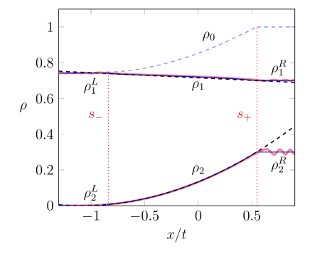
Figure 2: We compare the density field $\rho(c=x/t)$ for the numerical solution of the GP equations (1) (red lines) with the numerical solution of the Ovsyannikov equations (10) (blue lines) and the approximate analytical solution (17), (19) (black dashed lines). The vertical dotted lines indicate the edge velocities. The initial profile is characterized by $\rho_{1}^{L}=0.742$, $\rho_{2}^{L}=0$, $\rho_{1}^{R}=0.7$, $\rho_{2}^{R}=0.3$ and the interaction constants are equal to $g_{11}=g_{22}=g=1$, $g_{12}=\widetilde{g}=0.1$. The total density $\rho_{0}$ obtained by the numerical solution of the Ovsyannikov equations is shown by a blue dashed line. It is clear that this density is inhomogeneous in this case.

4.2 Approximate analytical solution of the Ovsyannikov equations

Now we suppose that one of the condensate components has a density much less than the density of the other component. To be definite, we assume that the first component has a greater density than the second component ($\rho_{1}\gg\rho_{2}$). In this case we can approximate $f$ given by equation (11) as

$$f\simeq-\frac{\sqrt{\rho_{2}}}{\sqrt{g_{11}g_{22}(1-v_{1}^{2})}\,v_{2}},\qquad g_{22}\rho_{2}\ll{g_{11}}\rho_{1}.$$ (16)

Substituting this expression in the second and fourth Ovsyannikov equations (10), we find that $v_{2}=v_{20}=\mathrm{const}$, where $v_{20}$ is defined by the initial condition. The density and the flow velocity of the second component are equal respectively to

$$\eqalign{\rho_{2}=\frac{1}{9g_{22}v_{20}^{2}}\left(2v_{20}\sqrt{g_{22}\rho_{20}}+u_{20}-c\right)^{2},\cr u_{2}=\frac{1}{3}\left(2v_{20}\sqrt{g_{22}\rho_{20}}+u_{20}+2c\right).}$$ (17)

Thus, in this approximation, we transform the system of four equations to a single equation that determines the dynamics of the first component,

$$\frac{3}{2}\frac{v_{1}}{\rho_{1}}\frac{d\rho_{1}}{dc}+\frac{dv_{1}}{dc}+\frac{1}{\sqrt{g_{11}\rho_{1}}}=0.$$ (18)

This equation can be reduced to the integral equation for the density and velocity of the first component

$$\rho_{1}^{3/2}v_{1}=\exp\left(\int_{c_{0}}^{c}\frac{dc}{v_{1}\sqrt{g_{11}\rho_{1}}}\right),$$

where the constant $c_{0}$ is determined by the initial conditions.

Let us return to the case when $g-\widetilde{g}\ll g$. For $\rho_{1}\gg\rho_{2}$ the density of the second component can be described approximately by the expression (17) with $u_{20}=0$. Since the total density is constant, the density of the first component is equal to $\rho_{1}(c)=\rho_{0}-\rho_{2}(c)$. This density distribution is shown in figure 1 by black dashed lines. It should be noted that the approximate solution describes well the structure even for not very large difference between $\rho_{1}$ and $\rho_{2}$.

In the case $\widetilde{g}\ll g$ the numerical solution suggests that the simple wave of the first component of the condensate has approximately a linear form,

$$\rho_{1}=a+bc.$$ (19)

Substituting this ansatz into expression (18), we obtain the differential equation

$$v_{1}^{\prime}+\frac{3b}{2(a+bc)}v_{1}+\frac{1}{\sqrt{g(a+bc)}}=0,$$ (20)

where the prime, as earlier, denotes the derivative with respect to $c$. Solution of this equation with the initial condition $v_{1}(c_{0})=v_{10}$ is given by

$$v_{1}=\left[\frac{a+bc_{0}}{a+bc}\right]^{3/2}\left(v_{10}+\frac{\sqrt{a+bc_{0}}}{2b\sqrt{g}}\right)+\frac{\sqrt{a+bc}}{2b\sqrt{g}}.$$ (21)

This expression determines the distribution of flow velocity along the simple wave. The parameter $b$ of the self-similar solution is the density derivative with respect to the characteristic velocity $c$ ($\rho_{1}^{\prime}=b$). Then we can write the equation for $b$ with the use of the Ovsyannikov equations as

$$b=\frac{2}{3v_{20}}\sqrt{\frac{\rho_{2}(\overline{c})(1-v_{20}^{2})}{g(1-v_{1}^{2}(\overline{c}))}},$$ (22)

where we have introduced a convenient variable $\overline{c}=(s_{-}+s_{+})/2$. Indeed, generally speaking, the plot of the rarefaction wave of the first component has a nonzero curvature. Therefore it seems reasonable to take the midpoint of this curve as a referent point for calculation of the mean slope of the straight line approximation. The constant $a$ can be found from the matching condition at the right edge of the rarefaction wave where it matches with the right plateau ($\rho_{1}(c_{0})={\rho}_{1}^{R}$),

$$a={\rho}_{1}^{R}+bv_{10}\sqrt{g{\rho}_{1}^{R}}.$$ (23)

Thus, after substitution of (23) into (22), we can find the parameters of the self-similar solution (19) by numerical solution of algebraic equation (22). figure 2 illustrates such an approximate structure where its comparison with the numerical solution of the GP equations (1) as well as with the numerical solution of the Ovsyannikov equations (10) and the approximate one (17), (19) are also given. It is clear that our approximate theory agrees with numerics very well.

As was mentioned above, if $\widetilde{g}\ll g$ and the continuity condition for the first component is not fulfilled ($\rho_{1}^{L}\neq\rho_{1}(s_{-})$), then the multi-valued region arises in the solution of the Ovsyannikov equations. To consider such a situation, we assume here that the initial parameters satisfy the inequality $\rho_{1}^{L}>\rho_{1}(s_{-})$. A typical density profile of the emerging wave structure is shown in figure 3. According to this figure, in the second component there exists, as before, a rarefaction wave only. However, the structure of the first component becomes more complicated. This wave profile is similar to one obtained in evolution of the initial discontinuity in a single component condensate with boundary velocities equal to zero, where a dispersive shock wave, that is the oscillatory wave structures emerging in evolution of the condensate after wave breaking, is generated on the right side, a rarefaction wave on the left side, and a plateau in between. However, there is one difference between these two situations, namely, now the rarefaction wave is a composite one because it consists of two regions: $(a)$ in the left one there is no flow of the second component, and $(b)$ in the right region where are rarefaction waves in both components.

First, we shall find a rarefaction wave in the region where the density of the second component is equal to zero. The solution of such a problem is simplified considerably if we pass from the ordinary physical variables $\rho_{1}$, $u_{1}$ for the first component to the so-called Riemann invariants. For the equations (4) the Riemann invariants are well known and can be written as (see, e.g., [10])

$$r_{\pm}=u_{1}\pm 2\sqrt{g\rho_{1}}.$$ (24)

The dispersionless system (4) can be written in the following diagonal Riemann form,

$$\frac{\partial r_{\pm}}{\partial t}+V_{\pm}(r_{+},r_{-})\frac{\partial r_{\pm}}{\partial x}=0,$$ (25)

where the “Riemann velocities” are given by

$$V_{+}=\frac{3}{4}r_{+}+\frac{1}{4}r_{-},\qquad V_{-}=\frac{1}{4}r_{+}+\frac{3}{4}r_{-}.$$ (26)

It is easy to express the physical variables in terms of $r_{\pm}$

$$\rho_{1}=\frac{1}{16g}(r_{+}-r_{-})^{2},\qquad u_{1}=\frac{1}{2}(r_{+}+r_{-}).$$ (27)

For the self-similar solution one has $r_{\pm}=r_{\pm}(c)$ and the system (25) reduces to

$$\frac{dr_{\pm}}{dc}\cdot\left(V_{\pm}-c\right)=0.$$ (28)

A rarefaction wave is characterized by the fact that one of the Riemann invariants has a constant value along the flow. For the case shown in figure 3, the rarefaction wave propagates to the left. Hence, the following invariant is constant in it:

$$r_{+}=u_{1}+2\sqrt{g\rho_{1}}=2\sqrt{g\rho_{1}^{L}},$$ (29)

where we set its value equal to the value at the boundary with the condensate at rest. The other Riemann invariant changes in such a way that the term in parentheses in the equation (28) with lower sign is equal to zero, $V_{-}=c$, what yields

$$\eqalign{\rho_{1}=\frac{1}{9g}\left(2\sqrt{g\rho_{1}^{L}}-\frac{x}{t}\right)^{2},\cr u_{1}=\frac{2}{3}\left(\sqrt{g\rho_{1}^{L}}+\frac{x}{t}\right).}$$ (30)

The left edge of this rarefaction wave propagates into the condensate at rest with the local sound velocity.

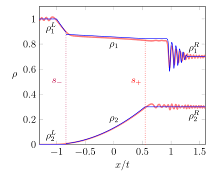
Figure 3: In this plot we compare the numerical simulations for the density field $\rho(c=x/t)$ obtained by numerical solution of the GP equations (1) (red lines) with the approximate solution (17), (19), (30), (33), (34) (blue lines). The vertical dotted lines denote the velocities of the edges. The initial profile is characterized by $\rho_{1}^{L}=1$, $\rho_{2}^{L}=0$, $\rho_{1}^{R}=0.7$, $\rho_{2}^{R}=0.3$ and the interaction constants are equal to $g_{11}=g_{22}=g=1$, $g_{12}=\widetilde{g}=0.1$. The wave structure in the first component consists of a dispersive shock wave on the right, two connected rarefaction waves on the left and a plateau between them. The second component has a single rarefaction wave only.

Since the interaction between the condensate components is small, we assume that the plateau and the dispersive shock wave can be found approximately as the structures resulting from evolution of only one component, i.e. we neglect here the interaction between the components. Along the plateau the invariant $r_{+}$ must have the same value as at the boundary between the rarefaction wave and the right plateau,

$$\overline{u}_{1}+2\sqrt{g\overline{\rho}_{1}}=2\sqrt{g\rho_{1}^{L}},$$ (31)

where $\overline{\rho}_{1}$ and $\overline{u}_{1}$ are the density and flow velocity in the plateau. After the passage through the dispersive shock wave the Riemann invariant $r_{-}$ retains its value which gives the relation

$$\overline{u}_{1}-2\sqrt{g\overline{\rho}_{1}}=-2\sqrt{g\rho_{1}^{R}}.$$ (32)

The equations (31), (32) allow one to find the densities and velocity of the components in the plateau region:

$$\overline{\rho}_{1}=\frac{1}{4}(\sqrt{\rho_{1}^{L}}+\sqrt{\rho_{1}^{R}})^{2},\quad\overline{u}_{1}=\sqrt{g\rho_{1}^{L}}-\sqrt{g\rho_{1}^{R}}.$$ (33)

Since the pioneering work of Gurevich and Pitaevskii (see [11]), it is known that wave breaking is regularized by the replacement of the nonphysical multi-valued dispersionless solution by a dispersive shock wave. This wave pattern can be represented approximately as a modulated nonlinear periodic wave

$$\eqalign{\rho_{1}=\frac{1}{4g}(\lambda_{4}-\lambda_{3}-\lambda_{2}+\lambda_{1})^{2}\cr\qquad+\frac{1}{g}(\lambda_{4}-\lambda_{3})(\lambda_{2}-\lambda_{1})\cr\qquad\times\mathrm{sn}^{2}(\sqrt{(\lambda_{4}-\lambda_{2})(\lambda_{3}-\lambda_{1})}\,\theta,m),\cr u_{1}=V-\frac{C}{g\rho_{1}},}$$ (34)

where

$$\eqalign{\theta=x-Vt,\quad V=\frac{1}{2}\sum_{i=1}^{4}\lambda_{i},\cr m=\frac{(\lambda_{2}-\lambda_{1})(\lambda_{4}-\lambda_{3})}{(\lambda_{4}-\lambda_{2})(\lambda_{3}-\lambda_{1})},\quad 0\leq m\leq 1;\cr C=\frac{1}{8}(-\lambda_{1}-\lambda_{2}+\lambda_{3}+\lambda_{4})\cr\times(-\lambda_{1}+\lambda_{2}-\lambda_{3}+\lambda_{4})(\lambda_{1}-\lambda_{2}-\lambda_{3}+\lambda_{4});}$$ (35)

and real parameters $\lambda_{i}$ are ordered according to the inequalities

$$\lambda_{1}\leq\lambda_{2}\leq\lambda_{3}\leq\lambda_{4}.$$

These parameters are slow functions of $x$ and $t$ along a dispersive shock wave. The periodic solution written in the form (34) has the advantage that the parameters $\lambda_{i}$ are the Riemann invariants of the Whitham modulation equations, and their evolution in our case is defined by the self-similar solution of the Whitham equations presented in a diagonal Riemann form (see [12, 13])

$$\frac{\partial\lambda_{i}}{\partial t}+V_{i}(\lambda_{1},\lambda_{2},\lambda_{3},\lambda_{4})\frac{\partial\lambda_{i}}{\partial x}=0,\quad i=1,2,3,4.$$ (36)

These equations describe the evolution of the parameters $\lambda_{i}$ and they can be derived by averaging a proper number of conservation laws. This method of deriving the modulation equations for nonlinear waves was proposed by Whitham (see [14, 15]). The velocities $V_{i}$ are expressed in terms of $K(m)$ and $E(m)$, complete elliptic integrals of the first and second kind, respectively (see [12, 13]). We need here only the expression for $V_{3}$,

$$V_{3}=\frac{1}{2}\sum_{i=1}^{4}\lambda_{i}-\frac{(\lambda_{4}-\lambda_{3})(\lambda_{3}-\lambda_{2})K(m)}{(\lambda_{3}-\lambda_{2})K(m)-(\lambda_{4}-\lambda_{2})E(m)},$$ (37)

As conserns the other Whitham velocities, it is important to notice that in the soliton limit $m\to 1$ (i.e., $\lambda_{3}\to\lambda_{2}$) the they reduce to

$$\eqalign{V_{1}(\lambda_{1},\lambda_{2},\lambda_{2},\lambda_{4})=\frac{3}{2}\lambda_{1}+\frac{1}{2}\lambda_{4},\cr V_{4}(\lambda_{1},\lambda_{2},\lambda_{2},\lambda_{4})=\frac{3}{2}\lambda_{4}+\frac{1}{2}\lambda_{1},}$$ (38)

In a similar way, in the small amplitude limit $m\to 0$ (i.e., $\lambda_{3}\to\lambda_{4}$) we obtain

$$\eqalign{V_{1}(\lambda_{1},\lambda_{2},\lambda_{4},\lambda_{4})=\frac{3}{2}\lambda_{1}+\frac{1}{2}\lambda_{2},\cr V_{2}(\lambda_{1},\lambda_{2},\lambda_{4},\lambda_{4})=\frac{3}{2}\lambda_{2}+\frac{1}{2}\lambda_{1}.}$$ (39)

This means that the edges of the dispersive shock wave match the smooth solutions of the hydrodynamic dispersionless approximation.

From a formal point of view, we look again for the self-similar solutions for the Whitham equations (36). Assuming that the $\lambda_{i}$’s depend only on the variable $c=x/t$, we obtain at once

$$\frac{d\lambda_{i}}{dc}\cdot\left(V_{i}(\lambda)-c\right)=0,\quad i=1,2,3,4.$$ (40)

Hence we find again that only one Riemann invariant varies along the dispersive shock wave, while the other three are constant.

From the matching conditions at the edges of the dispersive shock wave we find that at the soliton edge

$$\lambda_{1}=\overline{r}_{-}/2,\quad\lambda_{4}=\overline{r}_{+}/2\qquad\mbox{at}\qquad\lambda_{3}=\lambda_{2},$$ (41)

where $\overline{r}_{\pm}$ are the Riemann invariants of the dispersionless theory that are defined by the equations (24). Their values coincide with the values in the plateau at the soliton edge of the dispersive shock wave. Similarly, at the small-amplitude edge we find

$$\lambda_{1}=r_{-}/2,\quad\lambda_{2}=r_{+}/2\qquad\mbox{at}\qquad\lambda_{3}=\lambda_{4}.$$ (42)

Thus, the constant Riemann invariants are equal to

$$\lambda_{1}=-\sqrt{g\rho_{1}^{R}},\quad\lambda_{2}=\sqrt{g\rho_{1}^{R}},\quad\lambda_{4}=2\sqrt{g\rho_{1}^{L}}.$$ (43)

The $c$-dependence of $\lambda_{3}$ is determined by the condition of vanishing of the expression in brackets in equation (40),

$$V_{3}\left(-\sqrt{g\rho_{1}^{R}},\sqrt{g\rho_{1}^{R}},\lambda_{3},\frac{1}{2}\overline{u}_{1}+\sqrt{g\overline{\rho}_{1}}\right)=\frac{x}{t}.$$ (44)

Substitution of the values of $\lambda_{i}$ resulting from (43) and (44) into the periodic solution (34) yields the oscillatory dispersive shock wave structure for the physical variables $\rho$ and $u$ shown in figure 3.

The derived formulas also give the analytical expressions for the velocities of the edges of the dispersive shock wave. The soliton edge and the small-amplitude edge move, respectively, with the velocities

$$\eqalign{s_{-}^{(DSW)}=\frac{\sqrt{g}}{2}\left(\sqrt{\rho_{1}^{L}}+\sqrt{\rho_{1}^{R}}\right),\cr s_{+}^{(DSW)}=\frac{\sqrt{g}(2\rho_{1}^{L}-\rho_{2}^{R})}{\sqrt{\rho_{1}^{L}}}.}$$ (45)

These values also agree well with the results of our numerical calculation.

The rarefaction wave located in the region where the second component of the condensate forms also a rarefaction wave will be sought, as earlier, under the assumption that it has a linear shape (19). Here the parameter $a$ can be found from the matching condition of this rarefaction wave with the plateau

$$a={\rho}_{1}^{R}-b(\overline{u}_{1}-v_{10}\sqrt{g\overline{\rho}_{1}}).$$ (46)

From this condition and the expression (22) we can find numerically both parameters of the ansatz (19). As one can see, there is a slight difference between analytical results and numerical simulations for the simple wave and the dispersive shock wave. These deviations are associated with the neglect of interaction between the components of condensate.

5 Conclusion

In this paper, we have derived the differential equations witch describe the dynamics of simple waves in a two-component Bose-Einstein condensate without imposing restrictions on the relative interaction of these components. The theory is applied to the Riemann problem of evolution of an initial discontinuity for two specific cases of relatively strong and relatively weak repulsion between the components. In the first situation the rarefaction wave is formed only. It is found that in this situation the total density remains approximately uniform. In the other case, the appearance of more complex structures with formation of composite rarefaction waves, plateau and dispersive shock waves is demonstrated. We have found an approximate solution of this system where the density of particles in one of the components is mach greater than in the other one. Typical structures are described and it is shown that the analytical solutions are in good agreement with the numerical results.

References

References

- [1] Kevrekidis P G, Frantzeskakis D J and Carretero-Gonzalez R 2008 Emergent nonlinear phenomena in Bose-Einstein condensates (Berlin: Springer-Verlag).
- [2] Kivshar Yu S and Agrawal G P 2003 Optical solitons: From fibers to photoic crystals (San Diego: Academic Press).
- [3] Qu C, Pitaevskii L P and Stringari S 2016 Phys. Rev. Lett. 116 160402.
- [4] Ivanov S K, Kamchatnov A M, Congy T and Pavloff N 2017 Phys. Rev. E 96 062201.
- [5] Pitaevskii L P and Stringari S 2003 Bose-Einstein Condensatio (Oxford: Clarendon).
- [6] Ao P and Chui S T 1998 Phys. Rev. A 58 4836.
- [7] Ovsyannikov L V 1979 Zh. Prikl. Mekch. Tekchn. Fiz. 2 3 [1979 J. Appl. Mech. Techn. Phys. 30 127].
- [8] Verhaar B J, van Kempen E G M and Kokkelmans S J J M F 2009 Phys. Rev. A 79 032711.
- [9] Congy T, Kamchatnov A M and Pavloff N 2016 SciPost Phys. 1 006.
- [10] Kamchatnov A M 2000 Nonlinear periodic waves and their modulations (Singapore: World Scientific).
- [11] Gurevich A V and Pitaevskii L P 1973 Zh. Eksp. Teor. Fiz. 65 590-604 [1974 Sov. Phys. JETP 38 291-297].
- [12] Forest M G and Lee J E 1987 Oscillation Theory, Computation, and Methods of Compensated Compactness ed. by C. Dafermos et al. IMA Volumes on Mathematics and its Applications 2 (New York: Springer).
- [13] Pavlov M V 1987 Theoretical and Mathematical Physics 71 pp 584 588.
- [14] Whitham G B 1965 Proc. R. Soc. A 283 238.
- [15] Whitham G B 1974 Linear and Nonlinear Waves (New York: Wiley Interscience).