“Divide and Conquer” Semiclassical Molecular Dynamics: A practical method for Spectroscopic calculations of High Dimensional Molecular Systems

Abstract

We extensively describe our recently established “divide-and-conquer” semiclassical method [M. Ceotto, G. Di Liberto and R. Conte, Phys. Rev. Lett. 119, 010401 (2017)] and propose a new implementation of it to increase the accuracy of results. The technique permits to perform spectroscopic calculations of high dimensional systems by dividing the full-dimensional problem into a set of smaller dimensional ones. The partition procedure, originally based on a dynamical analysis of the Hessian matrix, is here more rigorously achieved through a hierarchical subspace-separation criterion based on Liouville’s theorem. Comparisons of calculated vibrational frequencies to exact quantum ones for a set of molecules including benzene show that the new implementation performs better than the original one and that, on average, the loss in accuracy with respect to full-dimensional semiclassical calculations is reduced to only 10 wavenumbers. Furthermore, by investigating the challenging Zundel cation, we also demonstrate that the “divide-and-conquer” approach allows to deal with complex strongly anharmonic molecular systems. Overall the method very much helps the assignment and physical interpretation of experimental IR spectra by providing accurate vibrational fundamentals and overtones decomposed into reduced dimensionality spectra.

I Introduction

The simulation of vibrational spectra of high-dimensional systems is an important open issue in quantum mechanics. The challenge is to beat the curse of dimensionality that plagues any quantum method in both electronic and nuclear spectroscopy simulations. In fact, the exact treatment of quantum problems often implies the set-up of a grid. As a consequence, the computational cost scales exponentially with dimensionality, and only simulations involving a few atoms can be exactly performed.(Bowman, Carrington, and Meyer, 2008; Avila and Carrington Jr, 2011a, b, 2012; Thomas and Carrington Jr, 2015) Alternatively, perturbative quantum methods have also been successfully applied to many systems, but they are intrinsically limited to a single reference geometry. (Barone, 2005; Puzzarini, Biczysko, and Barone, 2010, 2011; Biczysko et al., 2012; Bludsky et al., 2000; Bloino, Baiardi, and Biczysko, 2016) High dimensional systems, such as peptides, are instead usually simulated through ad-hoc scaled harmonic approaches or by means of classical mechanics, either using force fields(Petersen et al., 2005; Vanommeslaeghe et al., 2010; Wang et al., 2004) or employing ab initio molecular dynamics (AIMD)(Mathias et al., 2011; Gaigeot, 2010; Thomas et al., 2013; Gomez Llorente and Pollak, 1992; Iftimie, Minary, and Tuckerman, 2005; Pratihar et al., 2017; Schlegel et al., 2001) approaches in which the nuclear forces are calculated using electronic structure codes. In classical simulations the curse of dimensionality is significantly tamed with respect to quantum mechanical counterparts. However, a purely classical dynamics simulation is unable to describe tunneling effects, zero point energies, overtones and other important spectroscopic quantum features.

Semiclassical dynamics employs classical trajectories to reproduce quantum mechanical effects. In semiclassical methods, spectra are calculated in a time-dependent way, i.e. by Fourier transforming the survival amplitude or the autocorrelation function of some observables (such as the dipole moment).(Heller, 1981a) Semiclassical methods based on the coherent states Herman-Kluk propagator(Herman and Kluk, 1984; Antipov, Ye, and Ananth, 2015; Walton and Manolopoulos, 1995; Elran and Kay, 1999; Kay, 1994a, b, c) and the initial value representation (SCIVR)(Miller, 1970a, b; Church, Antipov, and Ananth, 2017) are robust, have been proven to reproduce quantum effects quite quantitatively,(Zhang and Pollak, 2004; Miller, 2001; Kay, 2005; Heller, 1981a; Shalashilin and Child, 2004; Bonnet and Rayez, 1997, 2004; Crespos et al., 2017; Gu and Garashchuk, 2016; Garashchuk, Rassolov, and Prezhdo, 2011; Conte and Pollak, 2010, 2012; Kondorskiy and Nanbu, 2015; Nakamura et al., 2016; Koda, 2015, 2016; Chapman and Cina, 2007; Chapman, Cheng, and Cina, 2011; Cheng and Cina, 2014; Grossmann and Xavier, 1998; Harabati, Rost, and Grossmann, 2004; Grossmann, 1999; Bonella, Montemayor, and Coker, 2005; Bonella, Ciccotti, and Kapral, 2010; Gottwald and Ivanov, ) and have been shown to have an accuracy in spectra calculations often within 1% of exact results.(Miller, 2005; Kay, 2005) Recently, the multiple-coherent (MC)-SCIVR technique has been developed. It allows to perform on-the-fly semiclassical molecular dynamics simulations given a few input trajectories.(Ceotto, Tantardini, and Aspuru-Guzik, 2011; Ceotto et al., 2009a, b; Ceotto, Dell‘ Angelo, and Tantardini, 2010; Conte, Aspuru-Guzik, and Ceotto, 2013; Gabas, Conte, and Ceotto, 2017; Ceotto, Zhuang, and Hase, 2013; Zhuang et al., 2012) The approach is amenable to ab initio direct molecular dynamics, thus avoiding the effort to construct an accurate analytical potential energy surface which may be quite demanding especially for large systems,(Braams and Bowman, 2009; Jiang and Guo, 2014; Conte, Qu, and Bowman, 2015; Homayoon et al., 2015; Paukku et al., 2013; Conte, Houston, and Bowman, 2015; Varga et al., 2016; Houston, Conte, and Bowman, 2016; Conte et al., 2013) and permits to faithfully reproduce quantum effects like quantum resonances,(Ceotto et al., 2009b) intra-molecular and long-range dipole splittings, and the quantum resonant ammonia umbrella inversion.(Conte, Aspuru-Guzik, and Ceotto, 2013) Nevertheless, all SCIVR methods run out of steam when straightforwardly applied to problems involving large-sized systems.

Understanding the reasons of such a limitation is the first step to do for dealing with the curse of dimensionality and possibly overcoming it. The semiclassical wavepacket for a system of $N$ degrees of freedom consists in the direct product of N monodimensional (Gaussian) wavefunctions $\left|\Psi\left(t\right)\right\rangle=\left|\psi_{1}\left(t\right)\right\rangle...\left|\psi_{N}\left(t\right)\right\rangle$. When the time-dependent overlap $\left\langle\Psi\left(0\right)|\Psi\left(t\right)\right\rangle$ is Fourier transformed to generate the spectrum, the simulation time should have been long enough to provide a significant overlap. In other words, if the trajectory does not periodically return to the surroudings of the phase space region where it started, a noisy signal will be collected. If, instead, the multidimensional classical trajectory is such that $\left(\mathbf{p}\left(t\right),\mathbf{q}\left(t\right)\right)$ approaches several times $\left(\mathbf{p}\left(0\right),\mathbf{q}\left(0\right)\right)$, then the overlap $\left\langle\Psi\left(0\right)|\Psi\left(t\right)\right\rangle$ is sizable and the signal associated to the vibrational features will prevail on the noise. The curse of dimensionality occurs because each monodimensional coherent state overlap $\left\langle\psi_{i}\left(0\right)|\psi_{i}\left(t\right)\right\rangle$ should be significant for all dimensions at the same time. Even for uncoupled oscillators with non-commensurable frequencies the concomitant overlapping event is rarer and rarer as the dimensionality increases, and the simulation time has to be much prolonged.(Ceotto, Tantardini, and Aspuru-Guzik, 2011) The present “divide et impera” idea starts from the consideration that a full-dimensional classical trajectory, once projected onto a sub-dimensional space, is more likely to provide a useful spectroscopic signal and for such a reduced dimensionality trajectory, a clear spectroscopic signal can be obtained in a much shorter amount of time with respect to the full-dimensional case, as we have recently shown.(Ceotto, Di Liberto, and Conte, 2017) Thus, according to this divide-and-conquer strategy, after dividing the full-dimensional space into mutual disjoint subspaces, a semiclassical spectroscopic calculation is performed separately for each subspace. While the classical trajectories are full-dimensional, the semiclassical calculations employ subspace information for calculating each partial spectrum. Composition of the projected spectra provides the full-dimensional one. Considering that nuclear spectra of high dimensional systems are often too crowded for an unambiguous interpretation, this “divide-and-conquer” strategy will also allow to better read and understand the physics behind the spectra and help the interpretation of experimental results.

In this paper we introduce some new features that significantly enhance the accuracy of our divide-and-conquer semiclassical initial value representation (DC SCIVR) method. Accuracy of results is estimated by comparison to exact values for systems up to 30 degrees of freedom (DOFs). In Section (II) we first recall the basics of time averaged semiclassical spectral density calculations,(Kaledin and Miller, 2003a, b) and then we describe in details the DC-SCIVR approach and two new subspace-separation criteria. In Section (III) we test the performance of DC SCIVR on strongly coupled Morse oscillators, real molecular systems like H₂O, CH₂O, CH₄, CH₂D₂, the very challenging Zundel cation (H₅O₂⁺) and, finally, the benzene molecule, which is, at the best of our knowledge, the highest dimensional molecular system for which exact quantum vibrational calculations have been performed.(Halverson and Poirier, 2015) A summary and some conclusions end the paper.

II A Divide and Conquer Strategy for Semiclassical Dynamics

This Section recalls the derivation of the DC-SCIVR expression for spectroscopic calculations. We start from the SC-IVR power spectrum formulation and its multiple coherent state time averaging implementation (MC-SCIVR), and then move to the “divide and conquer” working formula. Finally, we present three different techniques for partitioning the full-dimensional vibrational space into suitable lower-dimensional subspaces.(Ceotto, Di Liberto, and Conte, 2017)

II.1 The SC-IVR time averaged spectral density

We start by writing the power spectrum $\text{I}\left(E\right)$ of a molecular system, characterized by the Hamiltonian $\hat{H}$, as the Fourier transform of the survival amplitude(Heller, 1981a) of a given and arbitrary reference state $\left|\chi\right\rangle$

$$\text{I}\left(E\right)\equiv\frac{1}{2\pi\hbar}\int_{-\infty}^{+\infty}\left\langle\chi\left|e^{-i\hat{H}t/\hbar}\right|\chi\right\rangle e^{iEt/\hbar}dt.$$ (1)

In semiclassical (SC) molecular dynamics, the quantum time-evolution operator $e^{-i\hat{H}t/\hbar}$ of Eq. (1) is substituted by the stationary phase approximation to its Feynman Path Integral representation.(Feynman and Hibbs, 1965) In the position representation, the semiclassical propagator is a matrix whose elements are obtained as products of a complex action exponential and a stationary-phase pre-exponential factor, summed over all classical trajectories that connect the two endpoints.(Berry and Mount, 1972; Liu and Miller, 2007; Takahashi and Takatsuka, 2007; Tao and Miller, 2011; Garashchuk, Rassolov, and Prezhdo, 2011; Van Vleck, 1928; Gutzwiller, 1967; Baranger et al., 2001; Buchholz, Grossmann, and Ceotto, 2016; Yamamoto, Wang, and Miller, 2002) The search for these trajectories is hampered by the rigid double-boundary condition. In the SC-IVR dynamics, introduced by Miller and later also developed by Heller, Herman, Kluk, and Kay,(Miller, 1970b, a; Heller, 1981b, a; Kay, 1994a, b; Miller, 2001, 2005) the propagator is instead formulated in terms of classical trajectories determined by initial conditions $\left(\mathbf{p}\left(0\right),\mathbf{q}\left(0\right)\right)$ so that Eq. (1) becomes

$$\left\langle\chi\left|e^{-i\hat{H}t/\hbar}\right|\chi\right\rangle\approx\left(\frac{1}{2\pi\hbar}\right)^{F}\iintop d\mathbf{p}\left(0\right)d\mathbf{q}\left(0\right)C_{t}\left(\mathbf{p}\left(0\right),\mathbf{q}\left(0\right)\right)e^{\frac{i}{\hbar}S_{t}\left(\mathbf{p}\left(0\right),\mathbf{q}\left(0\right)\right)}\left\langle\chi\right.\left|\mathbf{p}\left(t\right)\mathbf{q}\left(t\right)\left\rangle\right\langle\mathbf{p}\left(0\right)\mathbf{q}\left(0\right)\right|\left.\chi\right\rangle,$$ (2)

where $F$ is the number of degrees of freedom, $S_{t}\left(\mathbf{p}\left(0\right),\mathbf{q}\left(0\right)\right)$ is the classical action, and $C_{t}\left(\mathbf{p}\left(0\right),\mathbf{q}\left(0\right)\right)$ indicates the pre-exponential stationary-phase factor. If $\left|\mathbf{p}\left(t\right),\mathbf{q}\left(t\right)\right\rangle$ is represented as a coherent state(Heller, 1981b, a, 1991; Shalashilin and Child, 2001) of the type

$$\left\langle\mathbf{x}|\mathbf{p}\left(t\right),\mathbf{q}\left(t\right)\right\rangle=\left(\frac{\text{det}\left(\Gamma\right)}{\pi^{F}}\right)^{1/4}e^{-\left(\mathbf{x}-\mathbf{q}\left(t\right)\right)^{T}\Gamma\left(\mathbf{x}-\mathbf{q}\left(t\right)\right)/2+i\mathbf{p}^{T}\left(t\right)\left(\mathbf{x}-\mathbf{q}\left(t\right)\right)/\hbar},$$ (3)

where $\Gamma$ is a diagonal width matrix with coefficients usually equal to the square root of the vibrational frequencies for bound states calculations, then the pre-exponential factor becomes

$$C_{t}\left(\mathbf{p}\left(0\right),\mathbf{q}\left(0\right)\right)=\sqrt{\text{det}\left|\frac{1}{2}\left(\frac{\partial\mathbf{q}\left(t\right)}{\partial\mathbf{q}\left(0\right)}+\frac{\partial\mathbf{p}\left(t\right)}{\partial\mathbf{p}\left(0\right)}-i\hbar\Gamma\frac{\partial\mathbf{q}\left(t\right)}{\partial\mathbf{p}\left(0\right)}+\frac{i}{\Gamma\hbar}\frac{\partial\mathbf{p}\left(t\right)}{\partial\mathbf{q}\left(0\right)}\right)\right|},$$ (4)

and Eq. (2) is commonly known as the Herman-Kluk survival amplitude of the Hamiltonian $\hat{H}$. However, for complex systems, the phase space integration of Eq. (2) requires too many trajectories to be feasible. To overcome this limitation, Miller and Kaledin introduced a time averaged version of the semiclassical propagator (TA-SCIVR),(Kaledin and Miller, 2003a, b) which significantly reduces the computational overhead

$$\text{I}\left(E\right) =\frac{1}{\left(2\pi\hbar\right)^{F}}\int\int d\mathbf{q}\left(0\right)d\mathbf{p}\left(0\right)\frac{\text{Re}}{\pi\hbar T}\int_{0}^{T}dt_{1}\int_{t_{1}}^{+\infty}dt_{2}e^{i\left(S_{t_{2}}\left(\mathbf{p}\left(0\right),\mathbf{q}\left(0\right)\right)+Et_{2}\right)/\hbar}$$

$$\times \langle\chi|\mathbf{p}(t_{2}),\mathbf{q}(t_{2})\rangle e^{-i\left(S_{t_{1}}\left(\mathbf{p}\left(0\right),\mathbf{q}\left(0\right)\right)+Et_{1}\right)/\hbar}\langle\mathbf{p}(t_{1}),\mathbf{q}(t_{1})|\chi\rangle C_{t_{2}}(\mathbf{p}(t_{1}),\mathbf{q}(t_{1})),$$ (5)

where $t_{1}$ is the additional time averaging variable and $t_{2}$ is the original Fourier transform variable. In Eq. (5) the integrand is time averaged by taking into account different portions of time length $t_{2}-t_{1}$ of the same trajectory started in $\left(\mathbf{p}\left(0\right),\mathbf{q}\left(0\right)\right)$. Considering that the pre-exponential factor is of the type $e^{i\omega t}$ for a harmonic $\omega$-frequency system, Eq. (4) can be reasonably approximated as $C_{t}\left(\mathbf{p}\left(0\right),\mathbf{q}\left(0\right)\right)=e^{i\phi_{t}}$, where $\phi_{t}=\mbox{phase}\left[C_{t}\left(\mathbf{p}\left(0\right),\mathbf{q}\left(0\right)\right)\right]$, leading to the computationally more convenient separable approximation version of TA-SCIVR (Kaledin and Miller, 2003a, b)

$$\text{I}\left(E\right)=\left(\frac{1}{2\pi\hbar}\right)^{F}\iintop d\mathbf{p}\left(0\right)d\mathbf{q}\left(0\right)\frac{1}{2\pi\hbar T}\left|\intop_{0}^{T}e^{\frac{i}{\hbar}\left[S_{t}\left(\mathbf{p}\left(0\right),\mathbf{q}\left(0\right)\right)+Et+\phi_{t}\right]}\langle\chi|\mathbf{p}\left(t\right),\mathbf{q}\left(t\right)\rangle dt\right|^{2}.$$ (6)

Eq. (6) is more amenable than (5) to phase space Monte Carlo integration, given the positive-definite integrand, and it has been tested with excellent results on several molecular systems. However, TA-SCIVR still requires thousands of trajectories per degree of freedom to reach convergence.(Kaledin and Miller, 2003a, b; Tamascelli et al., 2014; Di Liberto and Ceotto, 2016) To further reduce the computational effort, the multiple coherent time averaged SCIVR (MC SCIVR) has been introduced.(Ceotto, Tantardini, and Aspuru-Guzik, 2011; Ceotto et al., 2011, 2009a, 2009b; Ceotto, Dell‘ Angelo, and Tantardini, 2010; Conte, Aspuru-Guzik, and Ceotto, 2013) In the MC-SCIVR formulation, the reference state $\left|\chi\right\rangle$ is written as a combination of coherent states placed at the classical phase space points $\left(\mathbf{p}_{\text{eq}}^{i},\mathbf{q}_{\text{eq}}^{i}\right)$, i.e. $\left|\chi\right\rangle=\sum_{i=1}^{N_{\text{states}}}\left|\mathbf{p}_{\text{eq}}^{i},\mathbf{q}_{\text{eq}}^{i}\right\rangle$. $\mathbf{q}_{\text{eq}}^{i}$ is an equilibrium position, while $\mathbf{p}_{\text{eq}}^{i}$ is obtained in a harmonic fashion as $\left(p_{j,\text{eq}}^{i}\right)^{2}/2m=\hbar\omega_{j}\left(n+1/2\right)$, where j is a generic normal mode, $\omega_{j}$ is the associated frequency, and $m$ is unitary in mass-scaled normal mode coordinates. Eq.(6) has been shown to be quite accurate with respect to exact quantum mechanical simulations for the several molecules tested, even when applied to systems as complex as glycine.(Di Liberto and Ceotto, 2016; Conte, Aspuru-Guzik, and Ceotto, 2013; Tamascelli et al., 2014; Gabas, Conte, and Ceotto, 2017)

II.2 The “Divide-and-Conquer” strategy applied to semiclassical dynamics

In this Section we provide a more detailed explanation of the “divide-and-conquer” strategy previously introduced elsewhere.(Ceotto, Di Liberto, and Conte, 2017) The idea is to calculate the power spectrum $\text{I}\left(E\right)$ of Eq. (1) as composition of partial spectra $\widetilde{\text{I}}\left(E\right)$ each one calculated in a reduced M-dimensional phase space $\left(\tilde{\mathbf{p}},\tilde{\mathbf{q}}\right)$ of the full $\text{N}_{vib}$-dimensional space $\left(\mathbf{p},\mathbf{q}\right)\equiv\left(p_{1},q_{1,}...,\tilde{p}_{i+1},\tilde{q}_{i+1},...,\tilde{p}_{i+M},\tilde{q}_{i+M},...,p_{N_{vib}},q_{N_{vib}}\right)$. In quantum mechanics, where operators can be represented by matrices, the projection of an operator onto a sub-space is obtained by a preliminary suitable singular value decomposition (SVD),(Hinsen and Kneller, 2000) followed by a subsequent matrix multiplication between the full-dimensional operator and the projector. Semiclassically operators are represented in phase space coordinates and a suitable SVD is the one involving the displacement matrix $\mathbf{D}$ for the M-dimensional subspace.(Hinsen and Kneller, 2000; Harland and Roy, 2003) In our case, $\mathbf{D}$ is a $\mbox{N}_{\mbox{vib}}\times\mbox{M}$ dimensional matrix and a singular-value decomposition is obtained when $\mathbf{D}=\mathbf{U}\mathbf{\Sigma}\mathbf{V}$, where $\mathbf{U}$ is a $\mbox{N}_{\text{vib}}\times\mbox{M}$ matrix, $\Sigma$ is a $\mbox{M}\times\mbox{M}$ one, and $V$ a $\mbox{M}\times\mbox{M}$ one. The matrix $\Delta=\mathbf{U}\mathbf{U}^{T}$ is the projector onto the M-dimensional subspace. Eventually, any matrix $\mathbf{A}$ is projected onto the reduced M-dimensional subspace by taking $\tilde{\mathbf{A}}=\mathbf{\Delta}\mathbf{A}\mathbf{\Delta}$ and retaining the $\mbox{M}\times\mbox{M}$ sub-block of non-zero elements. Similarly, any vector $\mathbf{q}$ is projected by taking $\tilde{\mathbf{q}}=\mathbf{\Delta}\mathbf{q}$. Given these considerations, the projected power spectrum can be written as

$$\widetilde{I}\left(E\right)=\left(\frac{1}{2\pi\hbar}\right)^{M}\iintop d\tilde{\mathbf{p}}\left(0\right)d\tilde{\mathbf{q}}\left(0\right)\frac{1}{2\pi\hbar T}\left|\int_{0}^{T}e^{\frac{i}{\hbar}\left[\tilde{S}_{t}\left(\tilde{\mathbf{p}}\left(0\right),\tilde{\mathbf{q}}\left(0\right)\right)+Et+\tilde{\phi}_{t}\right]}\langle\tilde{\bm{\chi}}|\tilde{\mathbf{p}}\left(t\right),\tilde{\mathbf{q}}\left(t\right)\rangle dt\right|^{2},$$ (7)

where the M-dimensional coherent state in the M-dimensional sub-space is

$$\langle\mathbf{\tilde{x}|\tilde{\mathbf{p}}\left(t\right),\tilde{\mathbf{q}}\left(t\right)\rangle}=\left(\frac{\mbox{det}(\tilde{\Gamma})}{\pi^{M}}\right)^{\frac{1}{4}}e^{-\left(\mathbf{\tilde{x}}-\mathbf{\tilde{q}}\left(t\right)\right)^{T}\mathbf{\tilde{\Gamma}}\left(\mathbf{\tilde{x}}-\mathbf{\tilde{q}}\left(t\right)\right)/2+i\mathbf{\tilde{p}}^{T}\left(t\right)\left(\mathbf{\tilde{x}}-\mathbf{\tilde{q}}\left(t\right)\right)/\hbar}$$ (8)

where the matrix $\tilde{\Gamma}=\mathbf{U}\mathbf{U}^{T}\Gamma\mathbf{U}^{T}\mathbf{U}$ is the projected Gaussian width matrix. $\langle\mathbf{\tilde{x}}|\tilde{\chi}\rangle$ is obtained in a similar way. The phase space integration is now limited to $\int\int d\mathbf{\tilde{p}}\left(0\right)d\tilde{\mathbf{q}}\left(0\right)$, i.e. a 2M dimensional space. This greatly reduces the computational cost and the number of trajectories necessary to converge the Monte Carlo integration. Furthermore, the sampling of the initial conditions of the full-dimensional trajectories can be done according to a Husimi distribution in the subspace with the external degrees of freedom at equilibrium. The representation of the phase $\tilde{\phi}_{t}$ in reduced dimensionality is approximated as $\tilde{\phi}_{t}=\mbox{phase}\left[\tilde{C}_{t}\left(\tilde{\mathbf{p}}\left(0\right),\tilde{\mathbf{q}}\left(0\right)\right)\right]$, where the pre-exponential factor is calculated according to Eq.(4) and each matrix block is of the type $\partial\tilde{\bm{q}}\left(t\right)/\partial\tilde{\bm{q}}\left(0\right)$, and so on. The only component of Eq.(7) that cannot be projected onto the sub-space using the SVD is the classical action

$$\tilde{S}_{t}\left(\tilde{\mathbf{p}}\left(0\right),\tilde{\mathbf{q}}\left(0\right)\right)=\int_{0}^{T}\left[\frac{1}{2}m\dot{\tilde{{\bf q}}}^{2}\left(t\right)+V_{S}\left(\tilde{\bm{q}}\left(t\right)\right)\right]dt$$ (9)

since the expression of the “projected” potential $V_{S}\left(\tilde{\bm{q}}\left(t\right)\right)$ cannot be directly obtained. More specifically, the projected potential $V_{S}\left(\tilde{\bm{q}}\left(t\right)\right)$ should be the potential such that an M-dimensional trajectory starting with initial conditions $\left(\tilde{\mathbf{p}}\left(0\right),\tilde{\mathbf{q}}\left(0\right)\right)$ visits at all times $t$ the same phase-space points $\left(\tilde{\mathbf{p}}\left(t\right),\tilde{\mathbf{q}}\left(t\right)\right)$ obtained upon projection of the full-dimensional trajectory. However, the potential $V_{S}\left(\tilde{\bm{q}}\left(t\right)\right)$ is known only for systems characterized by a separable potential. In an effort to find a general and suitable expression for $V_{S}\left(\tilde{\bm{q}}\left(t\right)\right)$, we notice that the full-dimensional trajectory is continuous with continuous first derivatives for the full-dimensional molecular potential $V\left(\bm{q}\left(t\right)\right)$, and we deduce that the M-dimensional trajectory and $V_{S}\left(\tilde{\mathbf{q}}\left(t\right)\right)$ have the same features. In a straightforward way, we initially define the sub-dimensional potential as

$$V_{S}\left(\tilde{\mathbf{q}}\left(t\right)\right)\equiv V\left(\tilde{\mathbf{q}}\left(t\right);\mathbf{q}_{N_{vib}-M}\left(t\right)\right)$$ (10)

where the positions $\mathbf{q}_{N_{vib}-M}\left(t\right)$ belonging to the other subspaces have been downgraded to parameters. Then, we introduce a time-dependent field such that

$$V_{S}\left(\tilde{\mathbf{q}}\left(t\right)\right)=V\left(\tilde{\mathbf{q}}\left(t\right);\mathbf{q}_{N_{vib}-M}^{eq}\right)+\lambda\left(t\right),$$ (11)

since it is more intuitive and convenient to represent the reduced dimensionality potential in terms of the conditioned full-dimensional one (with the parametric coordinates in their equilibrium positions) plus an external time-dependent field. In agreement with our previous work,(Ceotto, Di Liberto, and Conte, 2017) we take the following expression for $\lambda\left(t\right)$

$$\lambda\left(t\right)=V\left(\tilde{\mathbf{q}}\left(t\right);\mathbf{q}_{N_{vib}-M}\left(t\right)\right)-\left[V\left(\tilde{\mathbf{q}}\left(t\right);\mathbf{q}_{N_{vib}-M}^{eq}\right)+V\left(\mathbf{q}_{M}^{eq};\mathbf{q}_{N_{vib}-M}\left(t\right)\right)\right]$$ (12)

which is exact in the separable limit. To verify this, we consider for simplicity a two dimensional separable potential of the type $V\left(q_{1}\left(t\right),q_{2}\left(t\right)\right)=V_{1}\left(q_{1}\left(t\right)\right)+V_{2}\left(q_{2}\left(t\right)\right)$ but the procedure is readily generalizable to separable potentials of any dimensionality. In the 2D case, using Eqs (11) and (12), we obtain $V_{S}\left(q_{1}\left(t\right)\right)=V_{1}\left(q_{1}\left(t\right)\right)-V_{1}\left(q_{1}^{eq}\right)$ which is exact. We also notice that in Eq. (12) an additional last term (the value of the instantaneous full-dimensional potential with the subspace coordinates at equilibrium) has been introduced with respect to Eq. (10). It provides a linear term in the action and consequently shifts the spectrum by a constant, allowing to match on the same scale each partial spectrum $\tilde{\text{I}}\left(E\right)$ and to obtain the full-dimensional spectrum $\text{I}\left(E\right)$ as a composition of the several $\tilde{\text{I}}\left(E\right)$. In this last aspect the DC-SCIVR procedure is somewhat similar to the one employed by Wehrle, Sulč and Vaníček in their reduced-dimensionality emission spectra simulations.(Wehrle, Sulc, and Vanicek, 2014) There, they exploited conservation of energy to derive a projected Lagrangian whose potential energy was made only of a constant term that had the effect to shift the total spectra. Finally, the full-dimensional DC-SCIVR zero point energy (ZPE) can simply be regained by summing up the partial ZPE contributions of each subspace.

To test the effectiveness of our scheme for $V_{S}\left(\tilde{\mathbf{q}}\left(t\right)\right)$, we consider two strongly coupled monodimensional Morse oscillators, whose analytical potential will be explicitly reported in Section III.1.

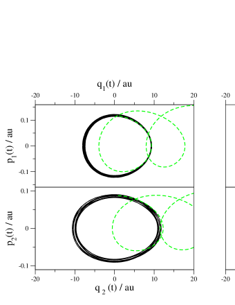
Figure 1: Mass-scaled phase space plot for the two strongly coupled Morse oscillators of Eq.(18). Left panel: Black continuous line for the exact, green dashed line for the potential $V_{S}\left(\tilde{\mathbf{q}}\left(t\right)\right)=V\left(\tilde{\mathbf{q}}\left(t\right);\mathbf{q}_{N_{vib}-M}^{eq}\right)$. Right panel: Black continuous line for the exact, red dashed line for the potential of Eq. (11).

Fig.(1) reports in the left panel the phase space plots for a classical trajectory with energy equal to that of the ground state. The black continuous line is for the $\left(\tilde{\mathbf{p}}\left(t\right),\tilde{\mathbf{q}}\left(t\right)\right)$ values obtained from the full-dimensional vector, which becomes $\left(\mathbf{p}\left(t\right),\mathbf{q}\left(t\right)\right)\equiv\left(p_{1}\left(t\right),q_{1}\left(t\right),p_{2}\left(t\right),q_{2}\left(t\right)\right)$ in this specific case, evolved according to the full-dimensional potential $V\left(\bm{q}\left(t\right)\right)$. The dashed green line is for the classical trajectory starting at $\left(\tilde{\mathbf{p}}\left(0\right),\tilde{\mathbf{q}}\left(0\right)\right)$ and evolved according to the approximate potential $V_{S}\left(\tilde{\mathbf{q}}\left(t\right)\right)=V\left(\tilde{\mathbf{q}}\left(t\right);\mathbf{q}_{N_{vib}-M}^{eq}\right)$, i.e without any $\lambda\left(t\right)$ correction. Such a potential is really unfit to describe the projected trajectory motion, since the green curve diverges after a few time-steps, as it were describing an unbound system. Two different phase-space plots for the same Morse oscillators appear on the right panel of Fig.(1). Again, the black continuous line is for the exact projected trajectory, while the dashed red line is for the classical trajectory starting at $\left(\tilde{\mathbf{p}}\left(0\right),\tilde{\mathbf{q}}\left(0\right)\right)$ and evolved according to the approximate potential $V_{S}\left(\tilde{\mathbf{q}}\left(t\right)\right)$ of Eq.(11). In this case, the trajectory phase-space plot is typical of a bound system. For one of the two dimensions, the phase space exact and approximate trajectories can be hardly distinguished. For the other degree of freedom, despite a phase accumulation, the frequency of the approximate trajectory motion is very similar to the exact one.

II.3 Vibrational space decomposition into mutually disjoint subspaces

It is now important to define an appropriate strategy for the decomposition of the full-dimensional space into mutually disjoint and convenient subspaces. The identification of relevant DOFs for spectroscopic calculations is a long-standing issue in spectroscopy, and several techniques to determine the “effective modes” have been proposed.(Picconi et al., 2013; Cederbaum, Gindensperger, and Burghardt, 2005) We present here three possible strategies: one is based on the time evolution of the Hessian matrix, and the other two on the evolution of the monodromy matrix. In all cases, a preliminary test trajectory is classically evolved starting from the atomic equilibrium positions and with initial kinetic energy equal to the harmonic zero point energy (ZPE) and distributed among the vibrational modes proportionally to their harmonic frequencies.

II.3.1 The Hessian space-decomposition method

We recall a decomposition strategy that has been recently presented(Ceotto, Di Liberto, and Conte, 2017) for the computation of molecular vibrational spectra. The full mass-scaled Hessian matrix is calculated at each time-step and the time averaged value of each Hessian matrix element is obtained, i.e. $\bar{H}_{ij}=\sum_{k=1}^{N}H_{ij}\left(t_{k}\right)/N$, with $N$ the number of time steps. If $\bar{|H}_{ij}|\geq\epsilon$, where $\epsilon$ is an arbitrarily fixed threshold parameter, then the degrees of freedom $i$ and $j$ are considered as belonging to the same subspace. If $|\bar{H}_{ij}|<\epsilon$, then $i$ and $j$ can still belong to the same subspace if there exists a third degree of freedom $k$ such that $\bar{H}_{ik}$ and $\bar{H}_{jk}$ are bigger than $\epsilon$. In that case, $i$ and $j$ (and also $k$) are collected into the same subspace. In Fig.(2) we report how the division into subspaces is affected by the chosen value of $\epsilon$. Clearly for $\epsilon=0$, all degrees of freedom are on the same full-dimensional space as shown in Fig.(2)(a).

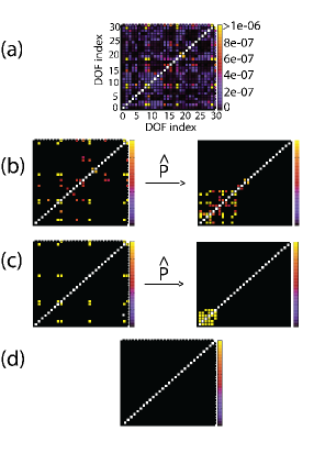
Figure 2: Hessian matrix elements for a system of 30 degrees of freedom (benzene) greater than a given threshold value $\epsilon$. The greater the value of $\epsilon$, the less dense is the matrix. Diagonal elements are out of scale and reported as white pixels. Panel (a) shows as pixels only the coupling elements that are greater than $\epsilon=0$ a.u. Panels (b), (c) and (d) are similar respectively for $\epsilon=4.5\cdot 10^{-7}$a.u., $\epsilon=9\cdot 10^{-7}$a.u. and $\epsilon=6\cdot 10^{-6}$a.u. In (b) and (c), the matrix elements have been conveniently arranged after permutations ($\hat{\mathbf{P}}$) into sub-blocks. Each sub-block determines a subspace.

By gradually increasing the value of $\epsilon$, the subspaces become more and more fragmented as illustrated in Fig.(2)(b) and (c). Finally, for $\epsilon$ bigger than a certain value, the full-dimensional space is broken down into a direct sum of mono-dimensional subspaces, as in Fig.(2)(d). In our simulations we usually choose a value of $\epsilon$ such that it maximizes the dimensionality of the biggest subspace provided that a spectroscopic signal can be collected and the curse of dimensionality does not kick in. This strategy is very advantageous in terms of computational effort, since the partition of the degrees of freedom into subspaces is instantaneous after the classical trajectory is run and the Hessian matrices calculated. However, there is no evidence that this strategy makes the partial spectra $\widetilde{\text{I}}\left(E\right)$ of Eq.(7) the most accurate with respect to the full-dimensional spectrum $\text{I}\left(E\right)$ of Eq.(6).

II.3.2 Wehrle-Sulč-Vaníček (WSV) space-decomposition method

An alternative decomposition approach (still based on dynamically averaged quantities and an arbitrary threshold) has been recently introduced by Vaníček and co-workers.(Wehrle, Sulc, and Vanicek, 2014) In fact, to quantify the coupling between various DOFs still in a dynamical way one can utilize the stability matrix. This is a $2N_{vib}$ dimensional matrix also called monodromy matrix and defined as

$$\bm{M}\left(t\right)\equiv\left(\begin{array}[]{cc}\partial\bm{p}\left(t\right)/\partial\bm{p}\left(0\right)&\partial\bm{p}\left(t\right)/\partial\bm{q}\left(0\right)\\ \partial\bm{q}\left(t\right)/\partial\bm{p}\left(0\right)&\partial\bm{q}\left(t\right)/\partial\bm{q}\left(0\right)\end{array}\right)=\left(\begin{array}[]{cc}\bm{M}_{\bm{pp}}&\bm{M}_{\bm{pq}}\\ \bm{M}_{\bm{qp}}&\bm{M}_{\bm{qq}}\end{array}\right)$$ (13)

It may be employed to measure how the classical energy is exchanged in time between the DOFs and, by virtue of Liouville’s theorem, its determinant is always equal to 1.

In their paper, Vaníček and co-workers define the following quantity $\mathbf{B}$ to measure the amount of coupling between the vibrational degrees of freedom in a dynamical fashion

$$B_{ij}=\left|\frac{\beta_{ij}}{\beta_{ii}}\right|,\;\text{with\>}\beta_{ij}=\frac{1}{T}\int_{0}^{T}dt\,(|M_{q_{i}q_{j}}(t)|+|M_{q_{i}p_{j}}(t)|+|M_{p_{i}q_{j}}(t)|+|M_{p_{i}p_{j}}(t)|),$$ (14)

where $\left|M_{ij}\left(t\right)\right|$ are the absolute values of the monodromy matrix elements of Eq. (13). After an arbitrary parameter $\epsilon_{B}$ is chosen, if the test $max\left\{B_{ij},B_{ji}\right\}\geq\epsilon_{B}$ is passed, then modes i and j go into the same subspace, following a procedure very similar to the one employed for our Hessian criterion but with the difference that more than a single threshold is used. In our calculations with the WSV method, given an $N_{vib}$ vibrational space, the bigger $M-$dimensional subspace is determined through a fixed value of $\epsilon_{B}$. For the remaining $N_{vib}-M$ DOFs, a different value of $\epsilon_{B}$ is chosen to obtain the biggest subspace between the remaining DOFs, and so on and so forth until all DOFs are grouped.

One might wonder if other dynamical quantities fit in the same general scheme made of a trajectory average followed by a comparison versus a threshold value. In this regard, the interested reader may find tests and a thorough discussion of several ways to define $\mathbf{B}$ on the basis of alternative averaged quantities (like, for instance, the correlation matrix of the wavepacket) in Wehrle’s doctoral thesis.(Wehrle, 2015)

II.3.3 Jacobi space-decomposition method

We here introduce a new approach to determine a subspace partition which leads to a more accurate calculation of $\widetilde{\text{I}}\left(E\right)$. Since in DC SCIVR the coherent state overlap $\langle\chi|\mathbf{p}\left(t\right),\mathbf{q}\left(t\right)\rangle$ is already written in terms of direct mono-dimensional overlaps and the action $\tilde{S}_{t}\left(\tilde{\mathbf{p}}\left(0\right),\tilde{\mathbf{q}}\left(0\right)\right)$ is approximated according to Eqs. (9), (11) and (12), the best strategy is one that minimizes the error in decomposing the full-dimensional pre-exponential factor into a direct product of lower-dimensional ones so that $C_{t}\left(\mathbf{p}\left(0\right),\mathbf{q}\left(0\right)\right)\approx\prod_{i}^{N_{sub}}$ $\tilde{C}_{t,i}\left(\tilde{\mathbf{p}}\left(0\right),\tilde{\mathbf{q}}\left(0\right)\right)$, where $N_{sub}$ is the number of subspaces. To understand how to better proceed, we take a two-dimensional separable system. The pre-exponential factor (4), using Eq. (13), can be written as

$$C_{t}\left(\mathbf{p}\left(0\right),\mathbf{q}\left(0\right)\right)=\sqrt{\text{det}\left|\frac{1}{2}\left(\bm{M}_{\bm{qq}}+\bm{M_{pp}}-i\hbar\bm{\Gamma}\bm{M_{qp}}+\frac{i}{\bm{\Gamma}\hbar}\bm{M}_{\bm{pq}}\right)\right|}$$ (15)

In the case of a two-dimensional separable system, the matrix components of Eq.(13) are diagonal matrices

$$\bm{M}_{\bm{pp}}=\left(\begin{array}[]{cc}M_{p_{1}p_{1}}&0\\ 0&M_{p_{2}p_{2}}\end{array}\right);\;\;\bm{M}_{\bm{pq}}=\left(\begin{array}[]{cc}M_{p_{1}q_{1}}&0\\ 0&M_{p_{2}q_{2}}\end{array}\right)\>...\text{ etc}.$$ (16)

Since the determinant of a block diagonal matrix is equal to the product of the block determinants, in the case of a separable system the pre-exponential factor of Eq.(15) is given by the product of the pre-exponential factors of each dimension. This consideration suggests that the best sub-space division is the one that minimizes the off-diagonal terms of the monodromy components in Eq. (16). The elements of the monodromy matrix can be rearranged into the Jacobian matrix

$$\mathbf{J}\left(t\right)=\left(\begin{array}[]{cc}\partial\mathbf{q}_{t}/\partial\mathbf{q}_{0}&\partial\mathbf{q}_{t}/\partial\mathbf{p}_{0}\\ \partial\mathbf{p}_{t}/\partial\mathbf{q}_{0}&\partial\mathbf{p}_{t}/\partial\mathbf{p}_{0}\end{array}\right)$$ (17)

and, in the case of a separable system, the determinant of the full-dimensional Jacobian, $\mathbf{J}\left(t\right)$, is given by the product of the determinants of each sub-space Jacobian $\tilde{{\bf J}_{i}}\left(t\right)$, i.e. $\text{det}\left(\mathbf{J}\left(t\right)\right)=\prod_{i}^{N_{sub}}$$\text{det}\left(\mathbf{\widetilde{J}}_{i}\left(t\right)\right)$. By virtue of Liouville’s theorem $\text{det}\left(\mathbf{J}\left(t\right)\right)=1$ at anytime, i.e. $d\mathbf{p}\left(t\right)d\mathbf{q}\left(t\right)=d\mathbf{p}\left(0\right)d\mathbf{q}\left(0\right)$, and, for a separable system, $\text{det}\left(\mathbf{\mathbf{\widetilde{J}}}_{i}\left(t\right)\right)=1$ for the generic $i\text{-th}$ subspace, so that $d\mathbf{\widetilde{p}}_{t}^{i}d\mathbf{\widetilde{q}}_{t}^{i}=d\mathbf{\widetilde{p}}_{0}^{i}d\mathbf{\widetilde{q}}_{0}^{i}$. However, in general, $d\mathbf{\widetilde{p}}_{t}d\mathbf{\widetilde{q}}_{t}\neq d\mathbf{\widetilde{p}}_{0}d\mathbf{\widetilde{q}}_{0}$ and we need to look for the subspace partition which provides subspace Jacobians $\mathbf{\widetilde{J}}_{i}\left(t\right)$ with the closest determinants to one. Since the Jacobian is time dependent, the search for the more suitable subspace division and for the best grouping of the vibrational modes within the different subspaces also depends on time. The chosen set of M vibrational modes for a M-dimensional subspace is the one that makes the $\mathbf{\widetilde{J}}_{M}\left(t\right)$ determinant the closest to unity more often during the time evolution of the test trajectory, and we will refer to this procedure as the “Jacobi criterion” from now on. The selection of the best subspace dimensionality is instead performed in a hierarchical way starting from the full-dimensional space and then proceeding through the remaining degrees of freedom. More specifically, once the best M-dimensional grouping has been determined for each subspace of dimensionality $M\leq N_{vib}$, we choose the one for which the determinant of $\tilde{{\bf J}}_{M}\left(t\right)$ (averaged over the trajectory) is the closest to unity. Clearly, $M$ is acceptable if it permits to achieve Monte Carlo convergence in TA-SCIVR calculations in the subspace, so it cannot be too big, otherwise the curse of dimensionality still kicks in. The same procedure is then iteratively applied for the remaining degrees of freedom until all of them have been grouped in various subspaces. The final result is a separation of the full-dimensional space into subspaces, where each subspace preserves Liouville’s theorem with the best possible accuracy. The main drawback of the method is that it comes at a higher computational cost than the two previously described.

In the next Section, we will apply Eqs (11) and (7) to several systems and compare our results with available quantum mechanical vibrational eigenvalues.

III Results and Discussion

III.1 A model system: two strongly coupled Morse oscillators

To test the accuracy of Eq.(7), we consider a coupled system of the type

$$V\left(q_{1},q_{2}\right)=D\sum_{i=1}^{2}\left[1-e^{-\alpha_{i}\left(q_{i}-q_{i}^{eq}\right)}\right]^{2}+c\left(q_{1}-q_{1}^{eq}\right)^{2}\left(q_{2}-q_{2}^{eq}\right)^{2}$$ (18)

where the coupling is biquadratic, the dissociation energy $D=0.2\>a.u.$ is the same for each oscillator, $\alpha_{i}=\omega_{i}\sqrt{\mu/2D}$, $c=10^{-7}\mu^{2}$, and $q_{1}^{eq}=q_{2}^{eq}=0$. The reduced mass $\mu$ is that of the $\text{H}_{2}$ molecule, i.e. $\mu=918.975\>\text{a.u.}$, and the harmonic frequencies are 3,000 and 1,700 wavenumbers. The oscillators are strongly coupled as shown by the deviation of the vibrational eigenvalues from the uncoupled ones. In this case there are two monodimensional subspaces and, as anticipated, we sample the initial phase space conditions for the $\left(\tilde{\mathbf{p}}\left(t\right),\tilde{\mathbf{q}}\left(t\right)\right)$ trajectories according to a Husimi distribution for the internal degree of freedom using a Box-Muller sampling centered at ($\tilde{p}_{1}^{eq}=\sqrt{\omega_{1}}$,$\tilde{q}_{1}^{eq}$) or ($\tilde{p}_{2}^{eq}=\sqrt{\omega_{2}}$, $\tilde{q}_{2}^{eq}$), with the other (external) degree of freedom initially set at equilibrium. The projection of the reference state on the subspaces is $\left|\tilde{\chi}\right\rangle=\left|\sqrt{\omega_{i}},q_{i}^{eq}\right\rangle,\,\,\,i=\left\{1,2\right\}$. The potential of Eq. (18) provides quite a stringent test for the DC-SCIVR approach because of the artificial strong coupling. We simulate the full-dimensional and the partial-dimensional spectra both with single trajectories using the MC-SCIVR approach and with many trajectories by means of Husimi-sampled TA-SCIVR calculations. In this latter instance, we perform 10,000 trajectories 50,000 a.u. long per subspace.

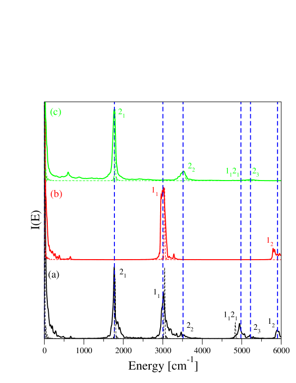
Figure 3: DC-SC-IVR spectra for the Morse oscillators of Eq. (18). Dashed lines are for the MC-SCIVR simulations and continuous ones for 10000-trajectory simulations. (a) black line for the full-dimensional TA-SCIVR spectrum; (b) red line for the DC-SCIVR spectrum of mode 1; (c) green line, the same of (b) for mode 2. Vertical dashed blue lines indicate the exact values calculated by a Discrete Variable Representation (DVR) approach.(Colbert and Miller, 1992)

The MC-SCIVR spectrum is losing accuracy only at high energies, since such energy range is not well sampled by MC SCIVR. In the partial spectra $\tilde{\text{I}}\left(E\right)$ in Fig. (3) the overtones generated by the quantum contribution from the other subspace are much less intense and barely detectable. Nevertheless, the main spectroscopic features, i.e. fundamentals and most of the overtones, are faithfully reproduced.

III.2 Small molecules: $\text{{H}}_{2}\text{{O}}$, $\text{{CH}}_{2}\text{{O}}$, CH₄, and $\text{{CH}}_{2}\text{{D}}_{2}$

We choose H₂O, CH₂O, CH₄, and CH₂D₂ as test cases for DC SCIVR, since these are molecular systems accessible to full-dimensional SCIVR calculations, as it has been shown in the past.(Kaledin and Miller, 2003a, b; Tamascelli et al., 2014; Di Liberto and Ceotto, 2016) We perform full-dimensional SCIVR and DC-SCIVR calculations using 30,000 a.u. long classical trajectories, which is a typical dynamics length for semiclassical calculations on molecules.(Tamascelli et al., 2014; Ceotto et al., 2009b; Gabas, Conte, and Ceotto, 2017)

Starting from H₂O, which is the smallest of these systems, we generate 12,000 classical trajectories on the potential energy surface of Partridge and Schwenke(Partridge and Schwenke, 1997) for the full dimensional TA-SCIVR calculations, while 4,000 trajectories per degree of freedom are sufficient in the case of DC-SCIVR spectra. As in the case of the Morse oscillators, the reference state of each M-dimensional subspace is $\left|\chi\right\rangle=\prod_{i}^{M}\left|\sqrt{\omega_{i}},q_{i}^{eq}\right\rangle$ , where $\omega_{i}$ is the harmonic frequency of the i-th normal mode of vibration included in the subspace. Harmonic frequencies are listed in the “HO” column of Table (1). By employing the three different subspace partition criteria previously illustrated, we find that the three vibrational degrees of freedom of water should always be grouped into two different subspaces. However, in the case of the Hessian approach modes 1 and 2 (the bending and symmetric stretch respectively) are separated from mode 3 (the asymmetric stretch), while the Jacobi and WSV methods suggest to collect together modes 2 and 3, leaving mode 1 alone. In Figure (4) the DC-SCIVR spectra of water obtained with the Jacobi criterion are presented, while Table (1) reports the detailed computed energy levels and compares them with full-dimensional SCIVR estimates and exact values.

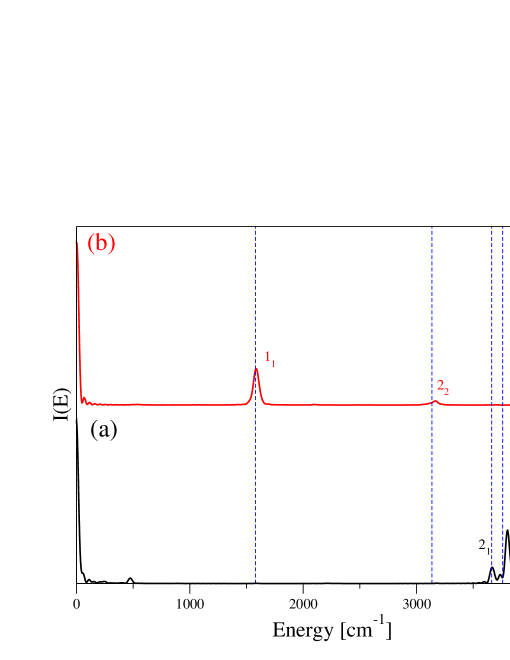
Figure 4: DC-SCIVR vibrational spectra of H₂O. The black line in panel (a) reports the two-dimensional subspace spectrum and the red line in panel (b) the monodimensional one. Vertical blue dashed lines are the full-dimensional TA-SCIVR values.

Table 1: Vibrational energy levels of water. The first and second columns show the vibrational state label and the exact results respectively; the third column reports the full-dimensional TA-SCIVR eigenvalues. Column four shows the DC-SCIVR results with the Jacobi subspace criterion (DC SCIVR${}_{\text{Jacobian}}$); column five refers to frequencies based on the WSV method (DC SCIVR${}_{\text{WSV}}$); in column six results obtained by employing the Hessian matrix criterion (DC SCIVR${}_{\text{Hess}}$) are listed. The last column reports the harmonic estimates. All values are in $\text{cm}{}^{-1}$. MAE stands for Mean Absolute Error and it is calculated with respect to the exact values,(Partridge and Schwenke, 1997) and for DC-SCIVR simulations also with respect to the full-dimensional TA-SCIVR values. Values for DC SCIVR${}_{\text{Jacobi}}$ and DC SCIVR${}_{\text{WSV}}$ are exactly the same because they are based on exactly the same partition of the vibrational modes into the two work subspaces.

Mode	Exact(Partridge and Schwenke, 1997)	TA SCIVR	DC SCIVR${}_{\text{Jacobi}}$	DC SCIVR${}_{\text{WSV}}$	DC SCIVR${}_{\text{Hess}}$	HO
$1_{1}$	1595	1580	1584	1584	1581	1649
$1_{2}$	3152	3136	3164	3164	3154	3298
$2_{1}$	3657	3664	3668	3668	3656	3833
$3_{1}$	3756	3760	3802	3802	3824	3944
MAE Exact		11	20	20	21	141
MAE SCIVR			20	20	23

First of all we observe that DC-SCIVR estimates generally account pretty well for the anharmonicity of water. This can be appreciated by comparing the mean absolute deviations from quantum exact values of the DC-SCIVR estimates (~ 20 cm^-1) to the mean deviation of the harmonic frequencies (~ 140 cm^-1). In spite of the anharmonicity and intermode coupling of water, all separation criteria offer rather accurate estimates. Only in the case of the asymmetric stretch fundamental frequency the partition procedure overestimates the quantum value, which is anyway very accurately regained by the full-dimensional semiclassical approximation.

Moving to CH₂O, we sample 24,000 classical trajectories to have the full-dimensional SCIVR calculation converged on the potential energy surface constructed by Martin et al.,(Martin, Lee, and Taylor, 1993). To keep the same overall computational cost, we take 4,000 trajectories per degree of freedom when calculating the partial spectra. The dimensionality of each subspace for the DC-SCIVR calculations is chosen by employing the three criteria introduced in Section (II). In the case of the Hessian matrix criterion, we find that for a value of $\epsilon=3.0\cdot 10^{-7}$ the full six-dimensional vibrational space is partitioned into a three-dimensional, a bi-dimensional and a mono-dimensional subspace. When using the WSV approach, the biggest subspace dimensionality is four for a threshold value of $\epsilon_{B}=120$. When employing the Jacobi criterion, the division turns out to be different.

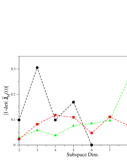
Figure 5: Average values of $\left|1-\text{det}\left(\tilde{\mathbf{J}}_{M}\left(t\right)\right)\right|$ for the best grouping for different subspace dimensionalities M. Black filled circles for CH₂O , red filled squares for CH₄, and green filled triangles for CH₂D₂.

Figure (5) shows the displacement of the determinant of the reduced-dimensional Jacobian matrix, i.e. $\text{det}\left(\tilde{\mathbf{J}}_{i}\left(t\right)\right)$ calculated on the basis of the projected trajectories $\tilde{\mathbf{p}}\left(t\right),\tilde{\mathbf{q}}\left(t\right)$, from unity for different choices of the subspace dimensionality M in the case of CH₂O, CH₄, and CH₂D₂. Clearly, there is no approximation for the full-dimensional analyses. For the CH₂O molecule, the smaller deviation is obtained for a maximum subspace dimensionality equal to 4, which is slightly better than a bi-dimensional choice. After fixing these four normal modes into the same subspace, the other two left modes are taken in the same subspace. Eventually the initial full-dimensional space is divided into 4- and 2- dimensional ones. The corresponding spectra are reported in Fig.(6).

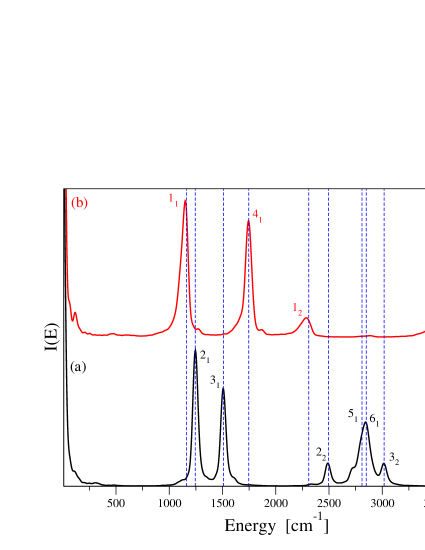
Figure 6: DC-SCIVR vibrational spectra of CH₂O. The black line in panel (a) reports the four-dimensional subspace spectrum and the red line in panel (b) the bi-dimensional one. Vertical blue dashed lines are the full-dimensional TA-SCIVR values.

As a comparison, the full-dimensional TA-SCIVR values are reported as vertical blue dashed lines. All vibrational features are faithfully reproduced, including overtones. It may be noticed that the signals of the fifth and sixth fundamentals sum up to a broader peak in the 4-dimensional spectrum. They can be separated by inserting the parity symmetry into the reference state when performing the 4-dimensional simulation. This common practice in semiclassical calculations permits to enhance the signal of one vibration at a time.(Kaledin and Miller, 2003b; Ceotto, Tantardini, and Aspuru-Guzik, 2011) To have a more detailed comparison Table (2) shows DC-SCIVR results, the exact ones,(Carter, Pinnavaia, and Handy, 1995) and the full-dimensional SCIVR frequencies.

Table 2: The same as in Table(1) this time for the vibrational energy levels of CH₂O.

Mode	Exact(Carter, Pinnavaia, and Handy, 1995)	TA SCIVR	DC SCIVR${}_{\text{Jacobi}}$	DC SCIVR${}_{\text{WSV}}$	DC SCIVR${}_{\text{Hess}}$	HO
$1_{1}$	1171	1162	1154	1154	1192	1192
$2_{1}$	1253	1245	1246	1246	1244	1275
$3_{1}$	1509	1509	1508	1508	1508	1544
$4_{1}$	1750	1747	1746	1746	1755	1780
$1_{2}$	2333	2310	2288	2288	2286	2384
$2_{2}$	2502	2497	2490	2490	2423	2550
$5_{1}$	2783	2810	2816	2816	2836	2930
$6_{1}$	2842	2850	2845	2845	2864	2996
$3_{2}$	3016	3018	3016	3016	3024	3088
$4_{2}$	3480	3476	3478	3478	3486	3560
MAE Exact		9	12	12	25	66
MAE SCIVR			6	6	19

To help the reader to better appreciate the level of accuracy for each semiclassical approximation, we report in the last lines the Mean Absolute Error (MAE). The DC-SCIVR deviation with respect to the exact value is $12\text{cm}^{-1}$ for the Jacobi and WSV approaches, and $25\text{cm}^{-1}$ for the Hessian one. These values are comparable with the full-dimensional TA-SCIVR one of $9\text{cm}^{-1}$. Conversely, a harmonic estimate is almost three times less accurate than the DC-SCIVR ones. When comparing the approximate DC-SCIVR results with the TA-SCIVR ones, the deviation is on average really small, respectively $6\text{cm}^{-1}$, $6\text{cm}^{-1}$ and $19\text{cm}^{-1}$ for the Jacobi, WSV, and Hessian criteria.

In the case of the CH₄ molecule, we employ the potential energy surface (PES) by Lee et al.(Lee, Martin, and Taylor, 1995) Given the highly chaotic regime for the classical trajectories of this PES, about 95% of the trajectories have been rejected due to the deviation of the full-dimensional monodromy matrix determinant from unity. By employing an amount of 180,000 trajectories, we still have enough trajectories left for TA-SCIVR Monte Carlo convergence. When dividing the space into subspaces, we keep the number of trajectories per degree of freedom equal to 20,000, in order to have for the overall DC-SCIVR calculation the same total amount of trajectories. We have recently shown (Ceotto, Di Liberto, and Conte, 2017) that when a value of $\epsilon=4.8\cdot 10^{-7}$ is employed for the Hessian criterion, the nine-dimensional vibrational space of methane is decomposed into six-dimensional and three-dimensional ones. When applying the WSV criterion with $\epsilon_{B}=85$, we also obtain a six-dimensional and a three dimensional subspace. Finally, even on the basis of the Jacobi criterion the better choice for the maximum dimensional subspace is six, as shown in Fig.(5). We then hierarchically apply the same criterion for the remaining vibrational modes and find out that a division into a bi-dimensional plus a mono-dimensional subspace is preferred with respect to a single three-dimensional one. Eventually, the nine-dimensional vibrational space is partitioned into six-, two- and mono-dimensional ones.

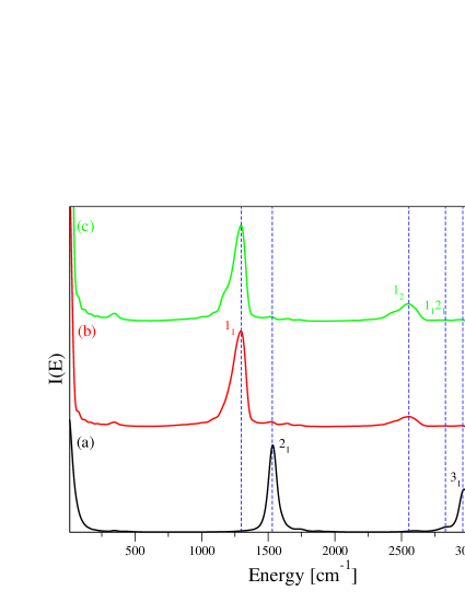
Figure 7: DC-SCIVR vibrational spectra of methane. Black line in panel (a) reports the six-dimensional subspace partial spectrum, the red line in panel (b) the bi-dimensional one, and the green line in panel (c) the mono-dimensional one. Vertical blue dashed lines indicate the full-dimensional TA-SCIVR values.

Fig.(7) reports the partial spectra of the three subspaces. Given the degeneracy of some of methane vibrations, the nine vibrational modes are labeled in four groups. Since degenerate modes can be projected onto different subspaces, spectral contributions to the same peak may be observed in Fig.(7) from different spectra. The full-dimensional TA-SCIVR peaks are once again well reproduced, including overtones and combination of overtones. Vibrations 4₁ and 2₂ have been separated by including the parity symmetry into the reference state. For a detailed comparison, we report in Table (3) our vibrational eigenvalues and compare them with the exact ones.

Table 3: The same as in Table(1) but for the vibrational energy levels of CH₄.

Mode	Exact(Carter, Shnider, and Bowman, 1999)	TA SCIVR	DC SCIVR${}_{\text{Jacobi}}$	DC SCIVR${}_{\text{WSV}}$	DC SCIVR${}_{\text{Hess}}$(Ceotto, Di Liberto, and Conte, 2017)	HO
$1_{1}$	1313	1300	1296	1308	1300	1345
$2_{1}$	1535	1529	1530	1530	1532	1570
$1_{2}$	2624	2594	2556	2588	2606	2690
$1_{1}2_{1}$	2836	2825	2830	2832	2834	2915
$3_{1}$	2949	2948	2960	2933	2964	3036
$2_{2}$	3067	3048	3060	3044	3050	3140
$4_{1}$	3053	3048	3056	3038	3044	3157
MAE Exact		12	17	15	11	68
MAE SCIVR			11	7	7

On average, the full-dimensional TA SCIVR is quite accurate, i.e. there is only a $12\text{cm}^{-1}$ difference from the exact frequency. The DC-SCIVR accuracy using the Jacobi criterion is slightly worse (MAE = $17\text{cm}^{-1}$), and it is comparable when using either the WSV or the Hessian criterion. These deviations are about six times more accurate than a crude harmonic approximation. Finally, a comparison among the different semiclassical approaches shows that in this case the Hessian criterion provides slightly more accurate results than the Jacobi ones. However, it is the overtone excitation $1_{2}$ which is responsible for the slightly worse accuracy of the Jacobi criterion with respect to the Hessian one. If one did not consider this term on the MAE calculation, the Jacobi DC SCIVR estimate would be on average within $9\text{cm}^{-1}$ of the exact one and only $6\text{cm}^{-1}$ away from the TA-SCIVR value.

Finally, we look at the lower symmetry molecule CH₂D₂, where some of the typical degenerations of methane have been removed. We employ the same PES as in the case of CH₄ and experience a comparable percentage of trajectory rejection for the monodromy matrix evolution in a chaotic potential. As above, we choose to employ 180,000 trajectories. Using the Hessian matrix criterion at a value $\epsilon=2\cdot 10^{-7}$ we obtain a decomposition of the full nine-dimensional space into a six-dimensional and a three-dimensional one. According to the WSV criterion, at a value $\epsilon_{B}=180$, we obtain a decomposition of the full nine-dimensional space into a four-dimensional, a three-dimensional and a bi-dimensional one. In the Jacobi approach reported in Fig.(5), we look at the green triangle profile and conclude that a four dimensional subspace is the first step in the hierarchical determination of the subspaces. Then, among the remaining five dimensional modes, the Jacobi analysis leads to a partition into a three- and a two-dimensional subspace. Eventually, the nine-dimensional space is divided into four, three and two dimensional subspaces.

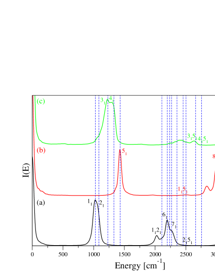
Figure 8: DC-SCIVR vibrational spectra of the CH₂D₂ molecule. The black line in panel (a) reports the partial spectrum for the 4-dimensional subspace, the red line in panel (b) the three-dimensional one and the green line in panel (c) the bi-dimensional one. Vertical blue dashed lines are the full-dimensional TA-SCIVR values.

Fig.(8) reports the partial spectra for the four-dimensional (a), the three-dimensional (b), and the two dimensional (c) subspaces. By comparison with the dashed vertical lines representing the full-dimensional semiclassical results we can observe that some accuracy is lost for the combined overtones (see the $1_{1}2_{1}$ peak) with respect to the typical accuracy of the fundamental peaks, as it was noticed for the strongly coupled Morse oscillators.

Table 4: The same as in Table(1) but for the vibrational energy levels of CH₂D₂.

Mode	Exact(Carter, Shnider, and Bowman, 1999)	TA SCIVR	DC SCIVR${}_{\text{Jacobi}}$	DC SCIVR${}_{\text{WSV}}$	DC SCIVR${}_{\text{Hess}}$	HO
$1_{1}$	1034	1026	1028	1020	1038	1053
$2_{1}$	1093	1084	1072	1098	1086	1116
$3_{1}$	1238	1230	1234	1212	1230	1266
$4_{1}$	1332	1329	1320	1326	1316	1360
$5_{1}$	1436	1430	1430	1420	1434	1471
$1_{1}2_{1}$	2128	2110	2089	2080	2114	2169
$6_{1}$	2211	2199	2195	2192	2137	2236
$1_{1}3_{1}$	2242	2236	2250	2231	2210	2319
$7_{1}$	2294	2268	2274	2250	2274	2336
$1_{1}4_{1}$	2368	2356	/	/	2400	2413
$1_{1}5_{1}$	2474	2456	2485	2436	2484	2524
$2_{1}5_{1}$	2519	2504	2516	2494	2510	2587
$3_{1}5_{1}$	2674	2660	2661	2672	2627	2737
$4_{1}5_{1}$	2769	2756	2754	2734	/	2831
$8_{1}$	3008	3050	3000	3012	3026	3103
MAE Exact		14	13	21	21	47
MAE SCIVR			12	15	19

Table (4) shows the computed DC-SCIVR energy levels which are compared with both the exact values (Carter, Shnider, and Bowman, 1999) and the full-dimensional TA-SCIVR ones. For this system, the MAEs relative to the exact values are more accurate for the TA-SCIVR and the Jacobian DC SCIVR than for the standard Hessian criterion. When comparing the different semiclassical approaches the expected order is found, i.e. from the more accurate TA SCIVR to the less accurate DC SCIVR.

III.3 A complex and strongly anharmonic molecular system: $\text{{H}}_{5}\text{{O${}_{2}^{+}$}}$

We keep proceeding in the application of DC-SCIVR to larger and larger molecules and face the challenge represented by the Zundel cation. H₅O₂⁺ with its 15 vibrational degrees of freedom has attracted the interest of many, mainly due to the vibrational features related to the motion of the shared proton. Specifically, a doublet is found in the vibrational pre-dissociation spectra of Zundel ions in the region of the O-H-O stretch associated to the proton transfer (~1000 cm^-1). Furthermore, two neatly separated bending signals are present owing to the water bending - proton transfer interaction.(Vendrell, Gatti, and Meyer, 2007a; Rossi, Ceriotti, and Manolopoulos, 2014) Consequently in our investigation we focus our attention on the proton transfer doublet, the water bendings, and, in addition, the four high-frequency free OH stretchings which are well detected by experimental spectra.(Hammer et al., 2005) We benchmark our DC-SCIVR simulations against the MCTDH calculations of Meyer et al. (Vendrell, Gatti, and Meyer, 2009a, b; Vendrell et al., 2009; Vendrell, Gatti, and Meyer, 2007b; Vendrell et al., 2007; Vendrell and Meyer, 2008; Vendrell, Gatti, and Meyer, 2007a) and also compare them with the VCI estimates of Bowman and collaborators.(McCoy et al., 2005)

We propagate the test classical trajectory on an accurate H₅O₂⁺ PES.(Huang, Braams, and Bowman, 2005) The trajectory is characterized by a strongly roto-vibrationally coupled motion leading to monodromy matrix instability and to a couple of hindrances to the application of our semiclassical techniques. For this reason, a Jacobi-based subspace partition is not feasible and we have to rely on the Hessian method to determine our work subspaces. Also, the coupling is responsible for an exaggerated broadening of the spectral features. This latter drawback can be overcome by removing the Cartesian angular momentum every few steps along the dynamics of the trajectories employed in our calculations. The associated loss in energy may partially affect the frequency accuracy (an artificial shift towards their harmonic counterparts is anticipated for the high frequencies) but it is compensated by the Husimi distribution of energies around the harmonic zero-point one employed for the initial conditions. Finally, due to the monodromy matrix instability, the original Herman-Kluk prefactor cannot be employed, so we approximate it by means of a reliable second order iterative approximation that depends only on the Hessian matrix.(Di Liberto and Ceotto, 2016) As expected, not only peaks in the spectra still have good accuracy but they are also much narrower thus decreasing the uncertainty of our results.

The Hessian criterion suggests us to enroll the normal modes associated to the free OH stretchings of the two water molecules into a four dimensional subspace, while all the other degrees of freedom are grouped into mono-dimensional subspaces. For this reason, we assign the two water bendings to two separate mono-dimensional subspaces, and the same fate applies to the mode associated to the shared proton motion. The only exception concerns the O-O stretching mode which is collected with a wagging state into a bi-dimensional subspace. This choice is driven by previous studies that have provided evidence of the occurrence of a combined state interacting with the shared proton motion.(Vendrell, Gatti, and Meyer, 2007a, 2009b) We run 2,000 full-dimensional classical trajectories per degree of freedom, i.e. 2,000 for the mono-dimensional subspaces, 4,000 for the bi-dimensional one, and 8,000 for the four-dimensional subspace. For each subspace, the initial kinetic energy is given in the usual harmonic fashion to the four OH stretches and to the modes enrolled in the subspace under investigation. No energy is instead given to the other modes.

Figure (9) reports the main excitations below 2,000 wavenumbers. To remove any spurious noise effect, we add a Gaussian filter of type $e^{-\alpha t^{2}}$ in the Fourier transform, with $\alpha=3\cdot 10^{-8}\>\text{a.u.}$ The orange and magenta lines refer to the two water bendings $\left(bu\right)$ and $\left(bg\right)$; the blue line shows the signal of the shared proton motion $\left(1z\right)$ and a mixed excitation$\left(1z,1R\right)$. Finally, on the bottom of the Figure are the spectra associated to the bi-dimensional subspace. The usual procedure based on selecting the parity of the semiclassical reference state permits to separate the overlapping features of this bidimensional subspace. Specifically, in green the fundamental for the O-O stretch $\left(1R\right)$ and its overtone $\left(2R\right)$ are detected, while in red the excitation $\omega_{3}$ of the wagging state (assigned on the basis of the MCTDH benchmark) and the combined excitation $\left(1R,\omega_{3}\right)$ stand out. In Figure (10) are instead illustrated the DC-SCIVR spectra of the free OH stretchings. In panel (a) the spectra of the $\left(sg\right)$ and $\left(su\right)$ excitations are reported, while panel (b) shows the signal of the two remaining OH stretchings labeled as $\left(sa\right)$.

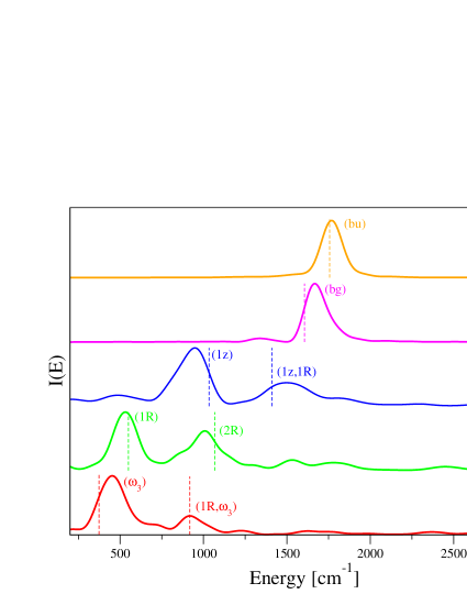
Figure 9: Vibrational spectra of the Zundel cation. Starting from the top, orange, magenta, and blue lines report the spectra of the mono-dimensional subspaces associate to the $\left(bu\right)$, $\left(bg\right)$, and $\left(1z\right)$ excitations; the green and red lines build up together the bi-dimensional subspace. The zero point energy value has been shifted to the origin in each subspace to help the reader in comparing the different frequencies. The vertical lines indicate the MCTDH reference.(Vendrell, Gatti, and Meyer, 2007a)

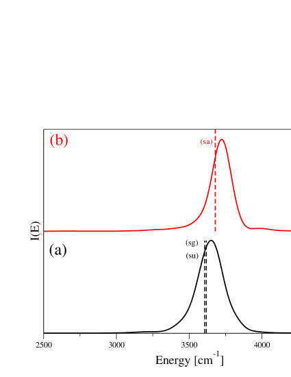
Figure 10: Vibrational spectra of the Zundel cation in the free OH stretching region. Starting from the bottom, panel (a) reports the spectrum of $\left(sg\right)$ and $\left(su\right)$, panel (b) refers to $\left(sa\right)$ excitations. The zero point energy value has been shifted to the origin to help the reader in evaluating the frequencies of the peaks. The vertical lines indicate the MCTDH estimates.(Vendrell, Gatti, and Meyer, 2007a)

Table (5) shows our computed energy levels, labeled with the usual nomenclature for the Zundel cation reported in the literature.(Vendrell, Gatti, and Meyer, 2007a, 2009b) Our DC-SCIVR estimates are pretty accurate with the exception of the combined excitation $\left(1z,1R\right)$ which is rather off-the-mark, but anyway better than the VCI value. A certain degree of inaccuracy arises also for the (1z) signal. As anticipated, the high frequency estimates are blue shifted with respect to the benchmark values, an effect the instantaneous removal of the Cartesian angular momentum may have largely contributed to. Overall, the average deviation from MCTDH results is 46 wavenumbers that decreases to 38 if $\left(1z,1R\right)$ is not considered. These values are not far from those found for smaller molecules and are satisfactory given the high complexity of the Zundel cation.

Table 5: Vibrational energy levels of the Zundel cation reported in cm^-1. The first column presents the label of the excitation according to Ref.(Vendrell, Gatti, and Meyer, 2007a) The second column contains the experimental values, the third and fourth ones show the MCTDH results from two different works,(Vendrell, Gatti, and Meyer, 2007a, 2009b) while in the fifth column our DC-SCIVR estimates are reported. Column six contains the VCI energy levels(McCoy et al., 2005) and, finally, in the last column are the harmonic estimates of the fundamental excitations. The last row reports the mean absolute error of the DC-SCIVR estimates with respect to the benchmark MCTDH values of Ref. Vendrell, Gatti, and Meyer, 2007a.

Label	Exp(Hammer et al., 2005)	MCTDH(Vendrell, Gatti, and Meyer, 2007a)	MCTDH(Vendrell, Gatti, and Meyer, 2009b)	DC SCIVR	VCI(McCoy et al., 2005)	HO
$\left(\omega_{3}\right)$${}^{\text{a}}$		374	386	452
(1R)		550		532		630
$\left(1R,\omega_{3}\right)$	928	918	913	920
(1z)	1047	1033	1050	952	1070	861
(2R)		1069		1008
$\left(1z,1R\right)$	1470	1411	1392	1520	1600
bg		1606		1668	1604	1720
bu	1763	1756	1756	1768	1781	1770
sg		3607		3650	3610	3744
su	3603	3614	3618	3650	3625	3750
sa	3683	3689	3680	3720	3698	3832
MAE				46

${}^{\text{a}}$This assignment of the $\omega_{3}$ wagging excitation is done upon comparison to the benchmark MCTDH values.

III.4 “Divide-and-Conquer” semiclassical dynamics for a high dimensional molecule: vibrational power spectrum of benzene

Halverson and Poirier have recently calculated the vibrational frequencies of benzene using a DVR approach. They pushed the limits of “exact” vibrational state calculations up to thirty dimensions.(Halverson and Poirier, 2015) In their method, the DVR basis set and grid has been conveniently selected using phase-space localized basis sets (PSLBs) and truncated Harmonic functions (HOB).(Avila and Carrington Jr, 2012, 2011b; Carter, Bowman, and Sharma, 2012) They were able to obtain all the relevant (about a million) vibrational energy levels of benzene within a given energy threshold. They employed a quartic force field modeling for the PES.(Handy et al., 1992)

We employ the same surface for a direct comparison between the present DC-SCIVR method and the exact DVR one. First we study how to best partition the 30-dimensional space. Using the Hessian-based approach and $\epsilon=9\cdot 10^{-7}$, the full-dimensional space is separated into one eight-dimensional, eight bi-dimensional and six mono-dimensional subspaces. When employing the WSV criterion and $\epsilon_{B}=5.6\cdot 10^{3}$, the full-dimensional space is partitioned into one ten-dimensional, two seven-dimensional and one six-dimensional subspace. When using the Jacobian-based criterion, the computational search for space decomposition is much more computationally expensive since all possible combinations of the 30 vibrational modes into groups of $M$ should be tested. We restrict instead our search to $6\leq M\leq 10$, since the Hessian criterion shows that when the biggest subspace is eight-dimensional then the results are quite accurate. We cannot rule out that there may be a better choice for $M>10$. However, the potential little improvement in the accuracy of the results does not justify the additional huge computational overhead.

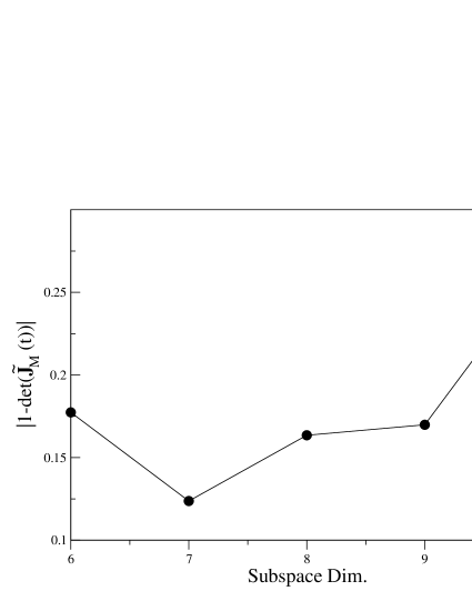
Figure 11: Values of $\left|1-\text{det}\left(\tilde{\mathbf{J}}_{M}\left(t\right)\right)\right|$ for different choices of the subspace dimensionality M for the $\text{C}_{6}\text{H}_{6}$ molecule.

Fig.(11) shows the result of this search and points to a seven-dimensional subspace for the first partition. The same procedure is repeated and involves the remaining 23 modes. The second subspace found is a six-dimensional one. The third search (among the remaining 17 modes) leads to a ten-dimensional subspace. The remaining seven modes are collected together within the same subspace. Eventually, the full thirty dimensional vibrational space has been partitioned into a ten-dimensional, two seven-dimensional, and one six-dimensional subspace. Whatever the method employed for partitioning the space, we run 1000 trajectories per degree of freedom to calculate the frequencies. Each trajectory is 30,000 a.u. long. To remove any spurious noise effect, in the Fourier transform we add the same Gaussian filter used for the Zundel cation. As usual, the reference state of each M-dimensional subspace is written as $\left|\chi\right\rangle=\prod_{i}^{M}\left|\sqrt{\omega_{i}},q_{i}^{eq}\right\rangle$ , where $\omega_{i}$ are the harmonic frequencies that we report under the columns “HO” in Table (6). For the evolution of the pre-exponential factor (4) and its phase calculation we use a recently introduced iterative second-order approximation.(Di Liberto and Ceotto, 2016) This approximation allows for the calculation of the pre-exponential factor without explicitly calculate the monodromy matrix elements, and it can be safely employed for strongly chaotic and high dimensional systems, as in the case of the benzene molecule.

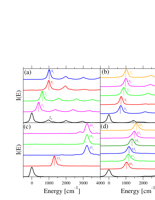
Figure 12: Vibrational spectra of C₆H₆ as obtained upon partition of the full-dimensional space according to the Jacobian criterion. Panel (a) reports the features of the six-dimensional subspace. Panels (b) and (c) contain the spectra of the two seven-dimensional subspaces, while panel (d) refers to the 10-dimensional subspace. The zero point energy value has been shifted to the origin to help the reader in evaluating the frequencies of the other peaks. The vertical lines indicate the exact levels from Poirier’s EQD calculations.(Halverson and Poirier, 2015)

Fig. (12) shows our computed spectra. Panel (a) reports the six-dimensional subspace, panels (b) and (c) the seven-dimensional ones, and panel (d) the 10-dimensional subspace.

Table 6: Benzene DC-SCIVR vibrational frequencies compared with available quantum results (EQD). Degenerate frequencies are not replicated. Values are given in $\text{cm}^{-1}.$

State	HO	DC SCIVR${}_{\text{WSV}}$	DC SCIVR${}_{\text{Jacobi}}$	EQD		State	HO	DC SCIVR${}_{\text{WSV}}$	DC SCIVR${}_{\text{Jacobi}}$	EQD
11	407	432	399	399.4554		111	1167	1150	1144	1147.751
21	613	610	606	611.4227		121	1192	1189	1175	1180.374
31	686	610	696	666.9294		22	1226	1223	1228	1221.27
41	718	742	719	710.7318		131	1295	1330	1314	1315.612
51	866	865	869	868.9106		141	1390	1375	1352	1352.563
61	989	990	997	964.0127		42	1436	1410	1437	1418.58
71	1011	1038	1020	985.8294		151	1512	1464	1492	1496.231
81	1008	1002	990	997.6235		161	1639	1614	1602	1614.455
91	1024	1014	1014	1015.64		52	1732	/	1752	1737.51
101	1058	1042	1042	1040.98		MAE		15	9

We follow Halverson and Poirier in their labeling of vibrational states. Table (6) reports our computed energy levels compared with the available exact ones. We find an excellent agreement with a MAE of only 9 wavenumbers when adopting Jacobi’s criterion. With the WSV approach, the MAE increases to $15\text{cm}^{-1}$. As we have recently reported,(Ceotto, Di Liberto, and Conte, 2017) the Hessian criterion leads to still acceptable but less accurate results, with a MAE of 19 wavenumbers.

Despite the increase in dimensionality, we conclude that moving from the three smaller molecular systems of the previous section to benzene, the MAE referred to the exact results is anyway limited to 10-20 $\text{cm}{}^{-1}$, a proof of the reliability of DC SCIVR and of the accuracy of the new Jacobian criterion.

IV Summary and Conclusions

All quantum mechanical methods suffer from the curse of dimensionality. In this paper we have illustrated a method to deal with it and to obtain vibrational frequencies almost as accurate as in standard SCIVR simulations, i.e. just a few wavenumbers away from the exact quantum values. More specifically, a “divide et impera” strategy has been adopted, in which spectra are calculated in partial dimensionality even if they are still based on full-dimensional classical trajectories. The method does not take advantage in any way of molecular symmetry.

We have shown how crucial the choice of the criterium for the decomposition of the full-dimensional space into mutually disjoint subspaces can be. In particular, the partition procedure based on the Jacobian matrix is the one that usually minimizes the error in approximating the full-dimensional pre-exponential factor as the direct product of several reduced dimensionality ones. This is evident from Fig. (13) where DC-SCIVR_Jacobi is clearly the overall more accurate way to decompose the vibrational space. The exception of CH₄ is due to a not very accurate estimate of a single overtone which we have anyway included in the MAE calculation, while the Jacobian-based partition strategy remains the most accurate even for CH₄ as far as fundamental frequencies are concerned. The apparent better accuracy of DC-SCIVR_Jacobi with respect to the full-dimensional calculation for CH₂D₂ is to be ascribed instead to an accidental compensation of errors between the semiclassical and subspace-partition approximations. Another key advantage of the Jacobian-based approach lies on its less noisy spectra with better resolved peaks, which is going to be more and more evident and helpful as the dimensionality of the system increases. Remarkably, the Jacobi criterion provides an internally consistent method to check the reliability of the subspace partition. In fact, not always an increase in the subspace dimensionality leads to more accurate vibrational frequencies. On the contrary, spectra can be noisier or it could be even impossibile to collect a sensible spectral signal. The partitioning schemes here developed can be also adopted for on-the-fly DC-SCIVR calculations. In fact, upon calculation of the test trajectory and of the associated Hessians and monodromy matrix elements by means of ab initio molecular dynamics, it is possible to determine the best subspace partition by following exactly the same procedures and at no additional cost with respect to DC-SCIVR simulations based on analytical potential energy surfaces.

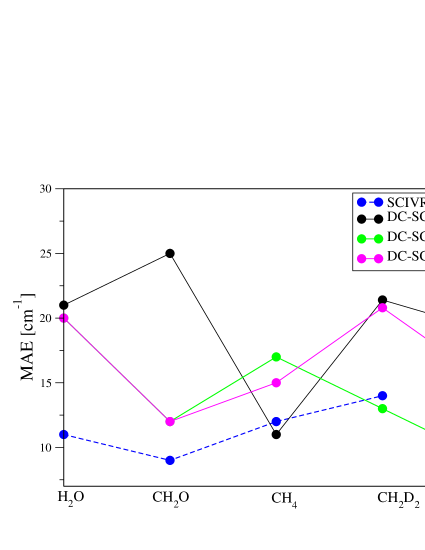
Figure 13: Trend of the mean absolute error (MAE) with respect to exact results for the different molecules investigated. Results refer to full-dimensional SC-IVR calculations (blue), DC SCIVR with Hessian matrix criterion (black), DC-SCIVR with Jacobian matrix criterion (green), and DC-SCIVR with WSV subspace partition (magenta).

DC-SCIVR, like other semiclassical and classical methods, is based on the Fourier transform of a survival amplitude. According to Nyquist’s theorem, for a total evolution time T a peak width equal to $2\pi/T$ should be expected. In our simulations, though, other factors contribute to increase the width of the spectral features. The ro-vibrational coupling generate a vibrational angular momentum which perturbs the pure vibrational motion. Furthermore, when a Gaussian filter is employed, peaks may be substantially enlarged (as in the case of H₅O₂⁺ and benzene). The full width at half maximum (FWHM) of the peaks provides a measure of the uncertainty of our results and benchmark values are always within this uncertainty bar. A potential drawback related to the width of the peaks is that it may hinder the resolution of spectral features very close to each other. A practical way to overcome this issue, that is largely adopted in semiclassical dynamics, consists in employing a proper combination of coherent states able to introduce a parity symmetry(Kaledin and Miller, 2003b; Tamascelli et al., 2014) which permits to distinguish among spectral features belonging to different vibrational modes.

A known issue of semiclassical spectra is represented by the so-called “ghost” peaks. These are unphysical features that can be generally distinguished from the true fundamental transitions because of their much lower intensity. As shown in Figure 3, this is not a specific drawback of DC-SCIVR simulations since full-dimensional calculations present the same issue. The adoption of a combination of coherent states able to account for the parity symmetry further enhances this discrepancy in the intensities making the identification of the true vibrational features even more favored.

DC SCIVR can be employed to simulate all kinds of spectroscopies relative to the nuclear motion, such as IR, Raman, absorption/emission dipole, vibro-electronic, and photodetachment spectra. It will allow to read each part of the spectra in a wider molecular context up to the nanoscale, with inclusion of non-trivial long-range quantum interactions. The calculation of partial spectra representations has not only the advantage to accelerate the Monte Carlo integration by virtue of the reduced dimensionality of each subspace and to get better resolved spectra, but also simplifies the identification of each peak. Another potential application of DC SCIVR is in the field of mixed (hybrid) semiclassical methods(Grossmann, 2006; Buchholz, Grossmann, and Ceotto, 2016, 2017) due to the possibility to assign different degrees of freedom to the different semiclassical techniques employed.

In conclusion, we think that semiclassical molecular dynamics is a very convenient approach for quantum mechanical simulations of nuclear vibrational spectroscopy. Future challenges, concerning the study of vibrational features of large molecules involved in biological mechanisms and technological processes, will be tackled in a novel quantum-mechanical fashion thanks to DC SCIVR and the implementation of the newly proposed subspace-separation criterion.

References

- Bowman, Carrington, and Meyer (2008) J. M. Bowman, T. Carrington, and H.-D. Meyer, Molecular Physics 106, 2145 (2008).
- Avila and Carrington Jr (2011a) G. Avila and T. Carrington Jr, J. Chem. Phys. 135, 064101 (2011a).
- Avila and Carrington Jr (2011b) G. Avila and T. Carrington Jr, J. Chem. Phys. 134, 054126 (2011b).
- Avila and Carrington Jr (2012) G. Avila and T. Carrington Jr, J. Chem. Phys. 137, 174108 (2012).
- Thomas and Carrington Jr (2015) P. S. Thomas and T. Carrington Jr, The Journal of Physical Chemistry A 119, 13074 (2015).
- Barone (2005) V. Barone, J. Chem. Phys. 122, 014108 (2005).
- Puzzarini, Biczysko, and Barone (2010) C. Puzzarini, M. Biczysko, and V. Barone, J. Chem. Theory Comput. 6, 828 (2010).
- Puzzarini, Biczysko, and Barone (2011) C. Puzzarini, M. Biczysko, and V. Barone, J. Chem. Theory Comput. 7, 3702 (2011).
- Biczysko et al. (2012) M. Biczysko, J. Bloino, I. Carnimeo, P. Panek, and V. Barone, J. Mol. Struct. 1009, 74 (2012).
- Bludsky et al. (2000) O. Bludsky, J. Chocholousova, J. Vacek, F. Huisken, and P. Hobza, J. Chem. Phys. 113, 4629 (2000).
- Bloino, Baiardi, and Biczysko (2016) J. Bloino, A. Baiardi, and M. Biczysko, Int. J. Quantum Chem. 116, 1543 (2016).
- Petersen et al. (2005) M. K. Petersen, F. Wang, N. P. Blake, H. Metiu, and G. A. Voth, J. Phys. Chem. B 109, 3727 (2005).
- Vanommeslaeghe et al. (2010) K. Vanommeslaeghe, E. Hatcher, C. Acharya, S. Kundu, S. Zhong, J. Shim, E. Darian, O. Guvench, P. Lopes, I. Vorobyov, et al., J. Comput. Chem. 31, 671 (2010).
- Wang et al. (2004) J. Wang, R. M. Wolf, J. W. Caldwell, P. A. Kollman, and D. A. Case, J. Comput. Chem. 25, 1157 (2004).
- Mathias et al. (2011) G. Mathias, S. D. Ivanov, A. Witt, M. D. Baer, and D. Marx, J. Chem. Theory. Comput. 8, 224 (2011).
- Gaigeot (2010) M.-P. Gaigeot, Phys. Chem. Chem. Phys. 12, 3336 (2010).
- Thomas et al. (2013) M. Thomas, M. Brehm, R. Fligg, P. Vöhringer, and B. Kirchner, Phys. Chem. Chem. Phys. 15, 6608 (2013).
- Gomez Llorente and Pollak (1992) J. Gomez Llorente and E. Pollak, Annu. Rev. Phys. Chem. 43, 91 (1992).
- Iftimie, Minary, and Tuckerman (2005) R. Iftimie, P. Minary, and M. E. Tuckerman, Proc. Natl. Acad. Sci. 102, 6654 (2005).
- Pratihar et al. (2017) S. Pratihar, X. Ma, Z. Homayoon, G. L. Barnes, and W. L. Hase, J. Am. Chem. Soc. 139, 3570 (2017).
- Schlegel et al. (2001) H. B. Schlegel, J. M. Millam, S. S. Iyengar, G. A. Voth, A. D. Daniels, G. E. Scuseria, and M. J. Frisch, J. Chem. Phys. 114, 9758 (2001).
- Heller (1981a) E. J. Heller, Acc. Chem. Res. 14, 368 (1981a).
- Herman and Kluk (1984) M. F. Herman and E. Kluk, Chem. Phys. 91, 27 (1984).
- Antipov, Ye, and Ananth (2015) S. V. Antipov, Z. Ye, and N. Ananth, J. Chem. Phys. 142, 184102 (2015).
- Walton and Manolopoulos (1995) A. R. Walton and D. E. Manolopoulos, Chem. Phys. Lett. 244, 448 (1995).
- Elran and Kay (1999) Y. Elran and K. Kay, J. Chem. Phys. 110, 3653 (1999).
- Kay (1994a) K. G. Kay, J. Chem. Phys. 101, 2250 (1994a).
- Kay (1994b) K. G. Kay, J. Chem. Phys. 100, 4432 (1994b).
- Kay (1994c) K. G. Kay, J. Chem. Phys. 100, 4377 (1994c).
- Miller (1970a) W. H. Miller, J. Chem. Phys. 53, 1949 (1970a).
- Miller (1970b) W. H. Miller, J. Chem. Phys. 53, 3578 (1970b).
- Church, Antipov, and Ananth (2017) M. Church, S. V. Antipov, and N. Ananth, J. Chem. Phys. 146, 234104 (2017).
- Zhang and Pollak (2004) D. H. Zhang and E. Pollak, Phys. Rev. Lett. 93, 140401 (2004).
- Miller (2001) W. H. Miller, J. Phys. Chem. A 105, 2942 (2001).
- Kay (2005) K. G. Kay, Annu. Rev. Phys. Chem. 56, 255 (2005).
- Shalashilin and Child (2004) D. V. Shalashilin and M. S. Child, Chem. Phys. 304, 103 (2004).
- Bonnet and Rayez (1997) L. Bonnet and J. Rayez, Chem. Phys. Lett. 277, 183 (1997).
- Bonnet and Rayez (2004) L. Bonnet and J.-C. Rayez, Chem. Phys. Lett. 397, 106 (2004).
- Crespos et al. (2017) C. Crespos, J. Decock, P. Larregaray, and L. Bonnet, J. Phys. Chem. C 121, 16854 (2017).
- Gu and Garashchuk (2016) B. Gu and S. Garashchuk, J. Phys. Chem. A 120, 3023 (2016).
- Garashchuk, Rassolov, and Prezhdo (2011) S. Garashchuk, V. Rassolov, and O. Prezhdo, Rev. Comput. Chem. 27, 287 (2011).
- Conte and Pollak (2010) R. Conte and E. Pollak, Phys. Rev. E 81, 036704 (2010).
- Conte and Pollak (2012) R. Conte and E. Pollak, J. Chem. Phys. 136, 094101 (2012).
- Kondorskiy and Nanbu (2015) A. D. Kondorskiy and S. Nanbu, J. Chem. Phys. 143, 114103 (2015).
- Nakamura et al. (2016) H. Nakamura, S. Nanbu, Y. Teranishi, and A. Ohta, Phys. Chem. Chem. Phys. 18, 11972 (2016).
- Koda (2015) S.-I. Koda, J. Chem. Phys. 143, 244110 (2015).
- Koda (2016) S.-I. Koda, J. Chem. Phys. 144, 154108 (2016).
- Chapman and Cina (2007) C. T. Chapman and J. A. Cina, J. Chem. Phys. 127, 114502 (2007).
- Chapman, Cheng, and Cina (2011) C. T. Chapman, X. Cheng, and J. A. Cina, J. Phys. Chem. A 115, 3980 (2011).
- Cheng and Cina (2014) X. Cheng and J. A. Cina, J. Chem. Phys. 141, 034113 (2014).
- Grossmann and Xavier (1998) F. Grossmann and A. L. Xavier, Phys. Lett. A 243, 243 (1998).
- Harabati, Rost, and Grossmann (2004) C. Harabati, J. M. Rost, and F. Grossmann, J. Chem. Phys. 120, 26 (2004).
- Grossmann (1999) F. Grossmann, Phys. Rev. A 60, 1791 (1999).
- Bonella, Montemayor, and Coker (2005) S. Bonella, D. Montemayor, and D. F. Coker, Proc. Natl. Ac. Sci. 102, 6715 (2005).
- Bonella, Ciccotti, and Kapral (2010) S. Bonella, G. Ciccotti, and R. Kapral, Chem. Phys. Lett. 484, 399 (2010).
- (56) F. Gottwald and S. D. Ivanov, https://arxiv.org/abs/1704.00477 .
- Miller (2005) W. H. Miller, Proc. Natl. Acad. Sci. USA 102, 6660 (2005).
- Ceotto, Tantardini, and Aspuru-Guzik (2011) M. Ceotto, G. F. Tantardini, and A. Aspuru-Guzik, J. Chem. Phys. 135, 214108 (2011).
- Ceotto et al. (2009a) M. Ceotto, S. Atahan, G. F. Tantardini, and A. Aspuru-Guzik, J. Chem. Phys. 130, 234113 (2009a).
- Ceotto et al. (2009b) M. Ceotto, S. Atahan, S. Shim, G. F. Tantardini, and A. Aspuru-Guzik, Phys. Chem. Chem. Phys. 11, 3861 (2009b).
- Ceotto, Dell‘ Angelo, and Tantardini (2010) M. Ceotto, D. Dell‘ Angelo, and G. F. Tantardini, J. Chem. Phys. 133, 054701 (2010).
- Conte, Aspuru-Guzik, and Ceotto (2013) R. Conte, A. Aspuru-Guzik, and M. Ceotto, J. Phys. Chem. Lett. 4, 3407 (2013).
- Gabas, Conte, and Ceotto (2017) F. Gabas, R. Conte, and M. Ceotto, J. Chem. Theory Comput. 13, 2378 (2017).
- Ceotto, Zhuang, and Hase (2013) M. Ceotto, Y. Zhuang, and W. L. Hase, J. Chem. Phys. 138, 054116 (2013).
- Zhuang et al. (2012) Y. Zhuang, M. R. Siebert, W. L. Hase, K. G. Kay, and M. Ceotto, J. Chem. Theory Comput. 9, 54 (2012).
- Braams and Bowman (2009) B. J. Braams and J. M. Bowman, Int. Rev. Phys. Chem. 28, 577 (2009).
- Jiang and Guo (2014) B. Jiang and H. Guo, J. Chem. Phys. 141, 034109 (2014).
- Conte, Qu, and Bowman (2015) R. Conte, C. Qu, and J. M. Bowman, J. Chem. Theory Comp. 11, 1631 (2015).
- Homayoon et al. (2015) Z. Homayoon, R. Conte, C. Qu, and J. M. Bowman, J. Chem. Phys. 143, 084302 (2015).
- Paukku et al. (2013) Y. Paukku, K. R. Yang, Z. Varga, and D. G. Truhlar, J. Chem. Phys. 139, 044309 (2013).
- Conte, Houston, and Bowman (2015) R. Conte, P. L. Houston, and J. M. Bowman, J. Phys. Chem. A 119, 12304 (2015).
- Varga et al. (2016) Z. Varga, R. Meana-Paneda, G. Song, Y. Paukku, and D. G. Truhlar, J. Chem. Phys. 144, 024310 (2016).
- Houston, Conte, and Bowman (2016) P. L. Houston, R. Conte, and J. M. Bowman, J. Phys. Chem. A (2016).
- Conte et al. (2013) R. Conte, B. Fu, E. Kamarchik, and J. M. Bowman, J. Chem. Phys. 139, 044104 (2013).
- Ceotto, Di Liberto, and Conte (2017) M. Ceotto, G. Di Liberto, and R. Conte, Phys. Rev. Lett. 119, 010401 (2017).
- Kaledin and Miller (2003a) A. L. Kaledin and W. H. Miller, J. Chem. Phys. 118, 7174 (2003a).
- Kaledin and Miller (2003b) A. L. Kaledin and W. H. Miller, J. Chem. Phys. 119, 3078 (2003b).
- Halverson and Poirier (2015) T. Halverson and B. Poirier, J. Phys. Chem. A 119, 12417 (2015).
- Feynman and Hibbs (1965) R. P. Feynman and A. R. Hibbs, Quantum mechanics and path integrals [by] RP Feynman [and] AR Hibbs (McGraw-Hill, 1965).
- Berry and Mount (1972) M. V. Berry and K. Mount, Rep. on Prog. Phys. 35, 315 (1972).
- Liu and Miller (2007) J. Liu and W. H. Miller, J. Chem. Phys. 127, 114506 (2007).
- Takahashi and Takatsuka (2007) S. Takahashi and K. Takatsuka, J. Chem. Phys. 127, 084112 (2007).
- Tao and Miller (2011) G. Tao and W. H. Miller, J. Chem. Phys. 135, 024104 (2011).
- Van Vleck (1928) J. H. Van Vleck, Proc. Natl. Acad. Sci. 14, 178 (1928).
- Gutzwiller (1967) M. C. Gutzwiller, J. Math. Phys. 8, 1979 (1967).
- Baranger et al. (2001) M. Baranger, M. A. de Aguiar, F. Keck, H.-J. Korsch, and B. Schellhaass, J. Phys. A 34, 7227 (2001).
- Buchholz, Grossmann, and Ceotto (2016) M. Buchholz, F. Grossmann, and M. Ceotto, J. Chem. Phys. 144, 094102 (2016).
- Yamamoto, Wang, and Miller (2002) T. Yamamoto, H. Wang, and W. H. Miller, J. Chem. Phys. 116, 7335 (2002).
- Heller (1981b) E. J. Heller, J. Chem. Phys. 75, 2923 (1981b).
- Heller (1991) E. J. Heller, J. Chem. Phys. 94, 2723 (1991).
- Shalashilin and Child (2001) D. V. Shalashilin and M. S. Child, J. Chem. Phys. 115, 5367 (2001).
- Tamascelli et al. (2014) D. Tamascelli, F. S. Dambrosio, R. Conte, and M. Ceotto, J. Chem. Phys. 140, 174109 (2014).
- Di Liberto and Ceotto (2016) G. Di Liberto and M. Ceotto, J. Chem. Phys. 145, 144107 (2016).
- Ceotto et al. (2011) M. Ceotto, S. Valleau, G. F. Tantardini, and A. Aspuru-Guzik, J. Chem. Phys. 134, 234103 (2011).
- Hinsen and Kneller (2000) K. Hinsen and G. R. Kneller, Mol. Simul. 23, 275 (2000).
- Harland and Roy (2003) B. B. Harland and P.-N. Roy, J. Chem. Phys. 118, 4791 (2003).
- Wehrle, Sulc, and Vanicek (2014) M. Wehrle, M. Sulc, and J. Vanicek, J. Chem. Phys. 140, 244114 (2014).
- Picconi et al. (2013) D. Picconi, F. J. A. Ferrer, R. Improta, A. Lami, and F. Santoro, Faraday discussions 163, 223 (2013).
- Cederbaum, Gindensperger, and Burghardt (2005) L. S. Cederbaum, E. Gindensperger, and I. Burghardt, Phys. Rev. Lett. 94, 113003 (2005).
- Wehrle (2015) M. Wehrle, Evaluation and analysis of vibrationally resolved electronic spectra with ab initio semiclassical dynamics, Ph. D. Thesis. (EPFL, 2015).
- Colbert and Miller (1992) D. T. Colbert and W. H. Miller, J. Chem. Phys. 96, 1982 (1992).
- Partridge and Schwenke (1997) H. Partridge and D. W. Schwenke, J. Chem. Phys. 106, 4618 (1997).
- Martin, Lee, and Taylor (1993) J. Martin, T. J. Lee, and P. Taylor, J. mol. spectr. 160, 105 (1993).
- Carter, Pinnavaia, and Handy (1995) S. Carter, N. Pinnavaia, and N. C. Handy, Chem. phys. lett. 240, 400 (1995).
- Lee, Martin, and Taylor (1995) T. J. Lee, J. M. Martin, and P. R. Taylor, J. Chem Phys. 102, 254 (1995).
- Carter, Shnider, and Bowman (1999) S. Carter, H. M. Shnider, and J. M. Bowman, J. Chem. Phys. 110, 8417 (1999).
- Vendrell, Gatti, and Meyer (2007a) O. Vendrell, F. Gatti, and H.-D. Meyer, J. Chem. Phys. 127, 184303 (2007a).
- Rossi, Ceriotti, and Manolopoulos (2014) M. Rossi, M. Ceriotti, and D. E. Manolopoulos, J. Chem. Phys. 140, 234116 (2014).
- Hammer et al. (2005) N. I. Hammer, E. G. Diken, J. R. Roscioli, M. A. Johnson, E. M. Myshakin, K. D. Jordan, A. B. McCoy, X. Huang, J. M. Bowman, and S. Carter, J. Chem. Phys. 122, 244301 (2005).
- Vendrell, Gatti, and Meyer (2009a) O. Vendrell, F. Gatti, and H.-D. Meyer, Angewandte Chemie International Edition 48, 352 (2009a).
- Vendrell, Gatti, and Meyer (2009b) O. Vendrell, F. Gatti, and H.-D. Meyer, J. Chem. Phys. 131, 034308 (2009b).
- Vendrell et al. (2009) O. Vendrell, M. Brill, F. Gatti, D. Lauvergnat, and H.-D. Meyer, J. Chem. Phys. 130, 234305 (2009).
- Vendrell, Gatti, and Meyer (2007b) O. Vendrell, F. Gatti, and H.-D. Meyer, Angewandte Chemie International Edition 46, 6918 (2007b).
- Vendrell et al. (2007) O. Vendrell, F. Gatti, D. Lauvergnat, and H.-D. Meyer, J. Chem. Phys. 127, 184302 (2007).
- Vendrell and Meyer (2008) O. Vendrell and H.-D. Meyer, Phys. Chem. Chem. Phys. 10, 4692 (2008).
- McCoy et al. (2005) A. B. McCoy, X. Huang, S. Carter, M. Y. Landeweer, and J. M. Bowman, “Full-dimensional vibrational calculations for h 5 o 2+ using an ab initio potential energy surface,” (2005).
- Huang, Braams, and Bowman (2005) X. Huang, B. J. Braams, and J. M. Bowman, J. Chem. Phys. 122, 044308 (2005).
- Carter, Bowman, and Sharma (2012) S. Carter, J. M. Bowman, and A. R. Sharma, in American Institute of Physics Conference Series, Vol. 1504 (2012) pp. 465–466.
- Handy et al. (1992) N. C. Handy, P. E. Maslen, R. D. Amos, J. S. Andrews, C. W. Murray, and G. J. Laming, Chem. Phys. Lett. 197, 506 (1992).
- Grossmann (2006) F. Grossmann, J. Chem. Phys. 125, 014111 (2006), http://dx.doi.org/10.1063/1.2213255.
- Buchholz, Grossmann, and Ceotto (2017) M. Buchholz, F. Grossmann, and M. Ceotto, J. Chem. Phys. 147, 164110 (2017).