Observation of the Unconventional Photon Blockade in the Microwave Domain

Abstract

We have observed the unconventional photon blockade effect for microwave photons using two coupled superconducting resonators. As opposed to the conventional blockade, only weakly nonlinear resonators are required. The blockade is revealed through measurements of the second order correlation function $g^{(2)}(t)$ of the microwave field inside one of the two resonators. The lowest measured value of $g^{(2)}(0)$ is 0.4 for a resonator population of approximately $10^{-2}$ photons. The time evolution of $g^{(2)}(t)$ exhibits an oscillatory behavior, which is characteristic of the unconventional photon blockade.

Photon blockade is observed when a single two-level emitter, such as an atom Birnbaum et al. (2005), a quantum dot Faraon et al. (2008), or a superconducting qubit Lang et al. (2011); Hoffman et al. (2011) is strongly coupled to a cavity, thus limiting the occupation of the cavity mode to zero or one photon. The second order correlation function $g^{(2)}(t)$ of the light leaking out of the cavity shows a dip at short time with $g^{(2)}(0)<1$, a signature of nonclassical fluctuations corresponding to antibunched photons. The same effect is predicted for a nonlinear Kerr cavity when the Kerr nonlinearity $U$ is much larger than the cavity linewidth $\kappa$ Imamoğlu et al. (1997). In 2010, Liew and Savona discovered that this constraint can be relaxed by considering two coupled cavities instead of one Liew and Savona (2010). They found that perfect blockade $g^{(2)}(0)=0$ can be achieved even for a vanishingly small ratio $U/\kappa$ and named the effect ”unconventional photon blockade” (UPB). The UPB was later interpreted as an interference between the two possible paths from the one to the two photon state Bamba et al. (2011) or as the fact that the cavity state is a displaced squeezed state Lemonde et al. (2014). Such states are known to exhibit antibunching for well-chosen displacement and squeezing parameters Stoler (1974); Mahran and Satyanarayana (1986); Lu and Ou (2001); Grosse et al. (2007). Reaching the strong coupling regime between a cavity and an emitter, or a large $U/\kappa$ in a Kerr cavity, remains highly challenging, especially in the optical domain. Therefore the UPB has attracted considerable attention Flayac and Savona (2017) by opening new possibilities to obtain sources of nonclassical light using readily available nonlinear cavities forming a photonic molecule Galbiati et al. (2012); Adiyatullin et al. (2017).

Figure 1: a) Microscope image of the two coupled Nb resonators used to observe the UPB. The bottom resonator is frequency tunable and slightly nonlinear due to the presence of a SQUID in the inductive arm. The SQUID consists of two Al/AlOx/Al Josephson junctions with a surface of 1 ${\rm\mu m}^{2}$ each. The blockade occurs in the top resonator, which is linear. The interdigited capacitance in the center couples the two resonators. The numbers label the ports connected to the sample. b) Evolution of the resonance frequency $\omega_{b}$ as a function of the SQUID flux. c) Evolution of $|S_{12}|^{2}$ as a function of frequency and SQUID flux. d) Microwave setup used to measure the UPB. Ports 3 and 4 are terminated by 50 $\Omega$ loads anchored at 10 mK. The LO signal is attenuated and pumps the system through the port 1. The signal of interest exits through port 2 and goes through two circulators and a diplexer before reaching the amplifier. After further amplification outside the cryostat, the signal is mixed with the LO and the resulting dc and ac components of each quadrature are filtered and digitized.

Here, we report on the observation of the UPB for microwave photons in a superconducting circuit consisting of two coupled resonators, one being linear and one weakly nonlinear Eichler et al. (2014). We measure the moments of the two quadratures of the field inside the linear resonator using a linear amplifier da Silva et al. (2010); Eichler et al. (2012). The determination of $g^{(2)}(0)$ for an arbitrary field requires measuring the moments of the two quadratures up to the fourth order. But in the case of the UPB, the state of the field is expected to be a displaced squeezed Gaussian state, therefore the value of $g^{(2)}(0)$ can be accurately obtained from the measurement of the first and second order moments only. This greatly reduces the experimental acquisition time and allows us to perform an exhaustive study of the blockade phenomenon as a function of various experimental parameters. In particular, we have searched for the optimal $g^{(2)}(0)$ as a function of the resonator population. We also measure $g^{(2)}(t)$ and observe oscillations that are characteristic of the UPB. Finally, we confirm the validity of the Gaussian assumption through measurements of the moments up to the fourth order.

Figure 1a shows a microscope image of the sample. Two resonators made of niobium and consisting of an inductance in series with a capacitance are coupled through a capacitance. The inductive part of the bottom resonator includes a SQUID that introduces a Kerr nonlinearity. Both resonators are coupled to two coplanar waveguides (CPW) that allow us to pump and probe the resonator fields. The effective Hamiltonian of the circuit is

$$H/\hbar=\omega_{a}a^{\dagger}a+\omega_{b}b^{\dagger}b+J(a^{\dagger}b+b^{\dagger}a)-Ub^{\dagger}b^{\dagger}bb,$$ (1)

where $\omega_{a}$ is the resonance frequency of the top resonator, $\omega_{b}$ is the resonance of the bottom resonator, which depends on the SQUID flux, $J$ the coupling and $U$ the Kerr nonlinearity. As shown in Bamba et al. (2011), this Hamiltonian leads to perfect blockade under the condition $\omega_{a}=\omega_{b}$ and $U=2\kappa^{3}/(3\sqrt{3}J^{2})$, where $\kappa$ is the loss rate of the resonators. The sample was designed to fulfill this condition with $J=2\pi\times 25$ MHz, $\kappa=2\pi\times 8$ MHz and $U=2\pi\times 0.3$ MHz.

To check these values for our sample, we first measure the evolution of $\omega_{b}$ with the SQUID flux as shown in figure 1b. We assume that the bottom resonator can be modeled by a lumped element circuit formed by the association in series of a capacitor $C$, an inductance $L$ and the SQUID inductance $L_{s}$, which varies with the applied flux $\phi$ as $L_{s}=L_{s0}/|\cos(\pi\phi/\phi_{0})|$. From the red fit, we obtain $L=1.09$ nH and $L_{s0}=81$ pH. When $\omega_{b}\approx\omega_{a}=2\pi\times 5.878$ GHz, we obtain $L_{s}=337$ pH, from which we deduce the Kerr nonlinearity $U=\pi p^{3}/(2R_{K}C)=2\pi\times 0.25$ MHz, where $R_{K}=h/e^{2}\approx 25.8\,{\rm k}\Omega$ and $p=L_{s}/(L+L_{s})$ Ong et al. (2011). Figure 1c shows a measurement of the top resonator transmission when $\omega_{b}$ crosses $\omega_{a}$. By fitting the observed avoided level crossing, we obtain $J=2\pi\times 25.1$ MHz. Finally, we have measured the linewidths (fwhm) of each resonator and obtained $\kappa_{a}=2\pi\times 10.35$ MHz for the top resonator and $\kappa_{b}=2\pi\times 7$ MHz for the bottom resonator.

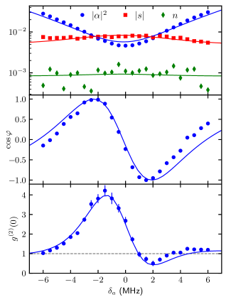
Figure 2: Evolution of $g^{(2)}(0)$ with the pump detuning. The two uppermost plots show the evolution of the Gaussian parameters characterizing the Gaussian state (see text) in the resonator as a function of $\delta_{a}$. Markers correspond to experimental data points and solid lines to the solution of the master equation Note (1). From these quantities, we compute $g^{(2)}(0)$ using equation (2). The error bars correspond to statistical $1\sigma$ errors. The nonlinear resonator is tuned to $\omega_{b}\approx\omega_{a}$ within a few MHz and the incident pump power on the sample is -107 dBm.

In order to measure the UPB, we make the assumption that the state in the resonator is Gaussian. This assumption is well verified in numerical simulations of the master equation describing our system in accordance with the predictions of Lemonde et al. (2014). Therefore, the quantum state of the resonator field $a$ is characterized by the displacement $\alpha=\langle a\rangle$ and by the Gaussian noise ellipse around the mean displacement. Defining the operator $d=a-\alpha$, the fluctuations of $d$ are Gaussian and are the one of a squeezed thermal state, which can be parametrized by the real number $n=\langle d^{\dagger}d\rangle$ and the complex number $s=\langle dd\rangle$. In the case of our experiment, because $s$ remains small, $n$ is the population of the thermal state. With these definitions, the second order correlation function at zero time is

$$g^{(2)}(0)=1+\frac{2|\alpha|^{2}(n+|s|\cos\varphi)+|s|^{2}+n^{2}}{(|\alpha|^{2}+n)^{2}},$$ (2)

where $\varphi$ is the complex argument of $s/\alpha^{2}$ Stoler (1974). This formula shows that a finite amount of squeezing is necessary to have $g^{(2)}(0)<1$. In the limit of a squeezed state with minimal uncertainty $n=0$ and supposing $|s|=|\alpha|^{2}$, one obtains $g^{(2)}(0)=2+2\cos\varphi$ showing that $g^{(2)}(0)$ oscillates with $\varphi$ between 0 and 4. Perfect antibunching is obtained when the state simultaneously fulfills the two conditions $|s|=|\alpha|^{2}$ and $\cos\varphi=-1$. Experimentally, one has to tune the pump and the nonlinear resonator frequencies to meet these conditions.

The measurement of $\alpha$, $n$ and $s$ is performed by amplifying the field leaving the top resonator with a cryogenic amplifier and by measuring the two quadratures of the amplified field as shown in figure 1d. We suppose that the field at the input of the IQ mixer is proportional to $a+h^{\dagger}$, where $h$ is a Gaussian field whose fluctuations are dominated by the intrinsic noise of the amplifier da Silva et al. (2010); Eichler et al. (2012). At the output of the mixer, we separate the ac and the dc components of each quadrature. The dc components $\bar{X}$, $\bar{Y}$ measure $\alpha$ while the ac components $X$, $Y$ are the quadratures of the field $d+h^{\dagger}$ at the pumping frequency. As shown in Ref. Lemonde et al. (2014), the noise spectrum of $d$ consists of two peaks centered approximately at $\pm J$ with a linewidth $\kappa$. We therefore filter the AC components with a bandpass filter of bandwidth $\Delta f=24$ MHz centered at 22.5 MHz.

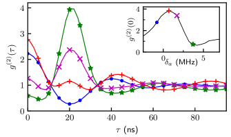
Figure 3: Measured time evolution of $g^{(2)}(\tau)$ for four different pump detunings. Solid lines interpolate the experimental data points. The bottom resonator is tuned to $\omega_{b}\approx\omega_{a}$ and the incident pump power is -101 dBm. Each curve corresponds to a different detuning $\delta_{a}$. The inset shows the evolution of $g^{(2)}(0)$ as a function of $\delta_{a}$, the four detunings corresponding to the curves in the main plot are identified by colored points. The oscillation of $g^{(2)}(\tau)$ with time is characteristic of the UPB. Depending on the initial phase of the oscillation, the state violates none, one or two of the inequalities $g^{(2)}(0)\geq 1$, $g^{(2)}(0)\geq g^{(2)}(\tau)$ that can be derived for a classical field.

The population of $h$ is $n_{h}=2k_{B}T_{\rm ampl}\Delta f/(G_{\rm att}\gamma_{2})$, where $T_{\rm ampl}=2$ K is the amplifier noise temperature, $G_{\rm att}=-3$ dB is the attenuation between the sample and the amplifier, and $\gamma_{2}=2\pi\times 8.6$ MHz is the simulated loss rate from the mode $a$ to the measurement port Note (1). These values lead to $n_{h}=12.5$, which must be compared to the expected values $|s|\approx 10^{-2}$ and $n\approx 10^{-3}$. In order to extract this small signal, we alternately acquire data turning the pump on and off and repeat this cycle many times. The period of the cycle is kept below 1 s to avoid any influence of a drift of the amplifier noise or gain. The expression of $\alpha$, $n$ and $s$ as a function of the measured moments are

$$\alpha = \frac{\langle\bar{X}\rangle_{1}+i\langle\bar{Y}\rangle_{1}}{\sqrt{2}}$$ (3a)

$$n = \frac{\langle X^{2}\rangle_{1}-\langle X^{2}\rangle_{0}+\langle Y^{2}\rangle_{1}-\langle Y^{2}\rangle_{0}}{2}+n_{\rm th}$$ (3b)

$$s = \frac{\langle X^{2}\rangle_{1}-\langle X^{2}\rangle_{0}-\langle Y^{2}\rangle_{1}+\langle Y^{2}\rangle_{0}}{2}+i\langle XY\rangle_{1}$$ (3c)

where $\langle\cdot\rangle_{1}$ ($\langle\cdot\rangle_{0}$) corresponds to averaged data when the pump is on (off). The data are rescaled to correct for the imperfections of the IQ mixer such that $\langle X^{2}\rangle_{0}=\langle Y^{2}\rangle_{0}=n_{h}$ and $\langle XY\rangle_{0}=0$ Note (1). By construction, the measurement of $n$ is only sensitive to a relative change of the fluctuations of the resonator field. We therefore have to make an assumption for the occupation of the measured mode when the pump is off. We suppose that the population is thermal with a mean occupation $n_{\rm th}$ that we calculate by estimating the incident thermal radiation on both resonators and solving the master equation Note (1). We obtain $n_{\rm th}=7.8\times 10^{-4}$, which corresponds to a temperature of 39.4 mK.

Figure 2 shows the results of the measurement of the Gaussian parameters $\alpha$, $n$ and $s$ when $\omega_{a}\approx\omega_{b}$ as a function of the detuning $\delta_{a}=\omega_{p}-\omega_{a}$ where $\omega_{p}$ is the pump frequency. The amplitude of the field $|\alpha|^{2}$ passes by a minimum when the detuning increases. Around this minimum, $|\alpha|^{2}$ is on the order of $|s|$ and $g^{(2)}(0)$ deviates significantly from one. The angle $\varphi$ determines the sign of the deviation and its evolution explains the oscillation of $g^{(2)}(0)$ around the resonance. The amount of squeezing is small and the Wigner distribution of the state is almost an isotropic Gaussian function. But because the displacement is also small, the squeezing is sufficient to make the overlap between the Wigner distribution of the state and the one of the two-photon Fock state smaller than for a coherent state. This happens when the small axis of the squeezing ellipse is aligned with the direction of the displacement $\alpha$ in the $XY$ plane, resulting in $g^{(2)}(0)<1$. Simulations of the master equation using the measured values for $U$,$J$,$\kappa_{a}$ and $\kappa_{b}$ well reproduce the observed evolution. The only adjustable parameter in the simulation is the pump intensity that we adjust to reproduce the observed displacement $|\alpha|^{2}$.

The Gaussian assumption can be extended to the measurement of $g^{(2)}(\tau)$ by introducing the time-dependent quantities $n(\tau)$ and $s(\tau)$. They are defined from the measured time-dependent correlation as in Eq. (3) with the transformation $\langle X^{2}\rangle\rightarrow\langle X(t)X(t+\tau)\rangle$, $\langle Y^{2}\rangle\rightarrow\langle Y(t)Y(t+\tau)\rangle$ and $\langle XY\rangle\rightarrow\langle X(t)Y(t+\tau)\rangle$. The results are plotted in figure 3 for four different pump frequencies. Because the squeezing results from the interference between the two components of the noise spectrum at $+J$ and $-J$, the angle $\varphi$ oscillates in time with a period $2\pi/J=40$ ns resulting in an oscillation of $g^{(2)}(\tau)$ that is characteristic of the UPB Liew and Savona (2010).

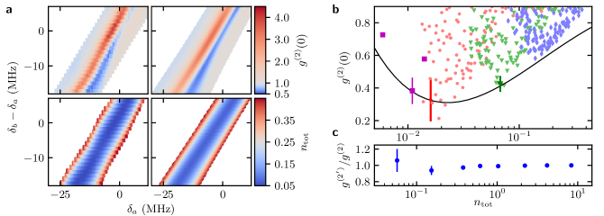
Figure 4: a) Evolution of $g^{(2)}(0)$ (top row) and $n_{\rm tot}$ (bottom row) as a function of the detuning $\delta_{a}$ and $\delta_{b}-\delta_{a}$. The left column shows experimental data that we compare to numerical simulations in the right column. The experimental pump power is -98 dBm and is adjusted in the simulation to reproduce the observed photon number. b) Evolution of $g^{(2)}(0)$ as a function of the resonator population. The light blue diamonds correspond to the dataset shown in a). The light red circles and green triangles correspond to two similar datasets measured at -104 and -101 dBm pump power respectively. The dark red and green points with 1$\sigma$ error bars correspond to the average of light red and green data points close to the minimum of $g^{(2)}(0)$. The magenta squares show measurements at fixed detunings, which should minimize $g^{(2)}(0)$ at low power, for three different powers (-107, -105, -104 dBm) and high statistics. The solid line is the prediction of the minimal $g^{(2)}(0)$ for our system Note (1) as a function of $n_{\rm tot}$. c) Experimental validation of the Gaussian state assumption. We have measured for fixed detunings all the moments of $X$ and $Y$ up to the fourth order for different pump strengths. We compute the second order correlation function with and without the Gaussian assumption and plot their ratio.

An important figure of merit for a single photon source is the evolution of $g^{(2)}(0)$ as a function of the source brightness, which is equal to $\gamma_{2}n_{\rm tot}$ where $n_{\rm tot}=|\alpha|^{2}+n$ is the resonator population. In order to minimize $g^{(2)}(0)$ for a given population, the pump strength, the pump frequency and the resonator detuning must be optimized. Experimentally, we fix the pump strength and measure $g^{(2)}(0)$ and $n_{\rm tot}$ varying both $\omega_{p}$ and $\omega_{b}$ as shown in figure 4a for one pump strength. By plotting the same data points as a function of $n_{\rm tot}$, we obtain a cloud of points whose lower envelope gives the minimal $g^{(2)}(0)$ as a function of $n_{\rm tot}$ for our system (see figure 4b). The solid line shows the predicted minimum. Its value decreases with $n_{\rm tot}$ and reaches a minimum when $n_{\rm tot}$ becomes of the order of $n_{\rm th}$ and then increases again when the thermal population dominates.

In figure 4b, we also show points with error bars that are obtained by averaging over a large number of measurements close to the minimum of $g^{(2)}(0)$ at a given pump power in order to obtain a better estimate of its value. We obtain $0.38\pm 0.08$, $0.33\pm 0.13$ and $0.43\pm 0.05$, respectively for the magenta, red, and green points. For these points, we now estimate the effect of a miscalibration in $n_{h}$ and $n_{\rm th}$ on the value of $g^{(2)}(0)$. Assuming an error of a factor two for both quantities, $g^{(2)}(0)$ varies between 0.18 and 0.76 for the magenta point, 0.17 and 0.63 for the red point and between 0.39 and 0.49 for the green point. The magenta point is very sensitive to a change in $n_{\rm th}$ because a large fraction of the resonator population is thermal. With increasing $n_{\rm tot}$ and smaller thermal fraction, the systematic error decreases.

Finally, we have checked the validity of the Gaussian assumption by measuring for a few points the moments of $X$ and $Y$ up to the fourth order. We then compute $g^{(2^{\prime})}(0)=\langle a^{\dagger}a^{\dagger}aa\rangle/\langle a^{\dagger}a\rangle^{2}$ and compare it to the value of $g^{(2)}(0)$ deduced from (2) as shown in figure 4c. Given the statistical error bars, the ratio $g^{(2^{\prime})}(0)/g^{(2)}(0)$ is consistent with one in the considered range of $n_{\rm tot}$. Simulations confirm that the Gaussian hypothesis is more and more valid with decreasing $n_{\rm tot}$ and we therefore expect the Gaussian assumption to be valid in the full range used in the experiment Note (1).

In conclusion, we have observed the main features of the UPB using two coupled superconducting resonators. We found a minimal value of $g^{(2)}(0)\approx 0.4$ which is limited by the thermal population in the cavity. An intriguing question is the extension of the UPB to a large number of coupled weakly nonlinear resonators and its role in the dynamics of coherently pumped lattices of superconducting resonators Houck et al. (2012).

Note added in proof. – Recently, we have become aware of a similar work in the optical domain Snijders et al. (2018).

References

- Birnbaum et al. (2005) K. M. Birnbaum, A. Boca, R. Miller, A. D. Boozer, T. E. Northup, and H. J. Kimble, Nature 436, 87 (2005).
- Faraon et al. (2008) A. Faraon, I. Fushman, D. Englund, N. Stoltz, P. Petroff, and J. Vučković, Nature Physics 4, 859 (2008).
- Lang et al. (2011) C. Lang, D. Bozyigit, C. Eichler, L. Steffen, J. M. Fink, A. A. Abdumalikov, M. Baur, S. Filipp, M. P. da Silva, A. Blais, and A. Wallraff, Physical Review Letters 106, 243601 (2011).
- Hoffman et al. (2011) A. J. Hoffman, S. J. Srinivasan, S. Schmidt, L. Spietz, J. Aumentado, H. E. Türeci, and A. A. Houck, Physical Review Letters 107, 053602 (2011).
- Imamoğlu et al. (1997) A. Imamoğlu, H. Schmidt, G. Woods, and M. Deutsch, Physical Review Letters 79, 1467 (1997).
- Liew and Savona (2010) T. C. H. Liew and V. Savona, Physical Review Letters 104, 183601 (2010).
- Bamba et al. (2011) M. Bamba, A. Imamoglu, I. Carusotto, and C. Ciuti, Phys. Rev. A 83, 021802 (2011).
- Lemonde et al. (2014) M.-A. Lemonde, N. Didier, and A. A. Clerk, Physical Review A 90, 063824 (2014).
- Stoler (1974) D. Stoler, Physical Review Letters 33, 1397 (1974).
- Mahran and Satyanarayana (1986) M. H. Mahran and M. V. Satyanarayana, Phys. Rev. A 34, 640 (1986).
- Lu and Ou (2001) Y. J. Lu and Z. Y. Ou, Physical Review Letters 88, 023601 (2001).
- Grosse et al. (2007) N. B. Grosse, T. Symul, M. Stobińska, T. C. Ralph, and P. K. Lam, Physical Review Letters 98, 153603 (2007).
- Flayac and Savona (2017) H. Flayac and V. Savona, Phys. Rev. A 96, 053810 (2017).
- Galbiati et al. (2012) M. Galbiati, L. Ferrier, D. Solnyshkov, D. Tanese, E. Wertz, A. Amo, M. Abbarchi, P. Senellart, I. Sagnes, A. Lemaître, E. Galopin, G. Malpuech, and J. Bloch, Physical Review Letters 108, 126403 (2012).
- Adiyatullin et al. (2017) A. F. Adiyatullin, M. D. Anderson, H. Flayac, M. T. Portella-Oberli, F. Jabeen, C. Ouellet-Plamondon, G. C. Sallen, and B. Deveaud, Nature Communications 8, 1329 (2017).
- Eichler et al. (2014) C. Eichler, Y. Salathe, J. Mlynek, S. Schmidt, and A. Wallraff, Physical Review Letters 113, 110502 (2014).
- da Silva et al. (2010) M. P. da Silva, D. Bozyigit, A. Wallraff, and A. Blais, Phys. Rev. A 82, 043804 (2010).
- Eichler et al. (2012) C. Eichler, D. Bozyigit, and A. Wallraff, Phys. Rev. A 86, 032106 (2012).
- Ong et al. (2011) F. R. Ong, M. Boissonneault, F. Mallet, A. Palacios-Laloy, A. Dewes, A. C. Doherty, A. Blais, P. Bertet, D. Vion, and D. Esteve, Physical Review Letters 106, 167002 (2011).
- Note (1) See Supplemental Material for details.
- Houck et al. (2012) A. A. Houck, H. E. Türeci, and J. Koch, Nature Physics 8, 292 (2012).
- Snijders et al. (2018) H. J. Snijders, J. A. Frey, J. Norman, H. Flayac, V. Savona, A. C. Gossard, J. E. Bowers, M. P. van Exter, D. Bouwmeester, and W. Löffler, Physical Review Letters 121, 043601 (2018).