The Star Formation Rate in the Gravoturbulent Interstellar Medium

Abstract

Stars form in supersonic turbulent molecular clouds that are self-gravitating. We present an analytic determination of the star formation rate (SFR) in a gravoturbulent medium based on the density probability distribution function of molecular clouds having a piecewise lognormal and power law form. This is in contrast to previous analytic SFR models that are governed primarily by interstellar turbulence which sets purely lognormal density PDFs. In the gravoturbulent SFR model described herein, low density gas resides in the lognormal portion of the PDF. Gas becomes gravitationally unstable past a critical density ($\rho_{crit}$), and the PDF begins to forms a power law. As the collapse of the cloud proceeds, the transitional density ($\rho_{t}$) between the lognormal and power law portions of the PDF moves towards lower-density while the slope of the power law ($\alpha$) becomes increasingly shallow. The star formation rate per free-fall time is calculated via an integral over the lognormal from $\rho_{crit}$ to $\rho_{t}$ and an integral over the power law from $\rho_{t}$ to the maximum density. As $\alpha$ becomes shallower the SFR accelerates beyond the expected values calculated from a lognormal density PDF. We show that the star formation efficiency per free fall time in observations of local molecular cloud increases with shallower PDF power law slopes, in agreement with our model. Our model can explain why star formation is spatially and temporally variable within a cloud and why the depletion times observed in local and extragalactic giant molecular clouds vary. Both star-bursting and quiescent star-forming systems can be explained without the need to invoke extreme variations of turbulence in the local interstellar environment.

1. Introduction

Stars are the fundamental link between galaxy evolution, planet formation, and astrobiology (Chyba & Hand, 2005; McKee & Ostriker, 2007; Krumholz, 2014). Stars inject energy and momentum into the surrounding interstellar and intergalactic medium, an effect commonly known as stellar feedback, via winds and supernova (Fall et al., 2010; Agertz et al., 2015; Lopez et al., 2011; Rosen et al., 2014, 2016; Hayward & Hopkins, 2017). Despite the importance of stars for galaxy evolution, a full observational and theoretical understanding of their formation remains elusive. If gravity alone was relevant, galactic interstellar clouds with density $\rho$ should collapse to form stars on roughly a free-fall time:

$$t_{ff}=\sqrt{3\pi/(32G\rho)}~{}~{};$$ (1)

However the dynamics of the star forming molecular interstellar medium are complicated by energetics that can counteract gravity, including magnetic fields and supersonic turbulence (Mouschovias & Spitzer, 1976; Larson, 1981; Shu et al., 1987; McKee et al., 1993; Mac Low & Klessen, 2004; McKee & Ostriker, 2007; Lazarian, 2007; Kowal et al., 2009; Crutcher et al., 2009a, 2010; Crutcher, 2012; Lazarian et al., 2012; Mocz et al., 2017), and the timescales for star formation are consequently much longer than the free-fall time. Additional factors that complicate our understanding of star formation include the many orders of magnitude in spatial and temporal scales and observational biases such as line-of-sight effects, limited resolution and incomplete density tracers (Goodman et al., 2009; Beaumont et al., 2015; Lombardi et al., 2015; Schneider et al., 2015a; Chen et al., 2017; Alves et al., 2017).

One of the main challenges for a theory of star formation is determining the star formation rate (SFR) and star formation efficiency (SFE) in both local molecular clouds and in galaxies (Krumholz, 2014). The current paradigm for the initial conditions of star formation is that stars form in dense filamentary molecular clouds that result from gravo-magnetohydrodyanmic (MHD)-turbulent fragmentation (Mac Low & Klessen, 2004; Krumholz & McKee, 2005; Padoan & Nordlund, 2011; Hennebelle et al., 2011; Federrath & Klessen, 2012; Federrath, 2013a; Collins et al., 2012; Hopkins, 2013; Burkhart & Lazarian, 2012; Lee et al., 2015; Semenov et al., 2016; Mocz et al., 2017; Semenov et al., 2017). The initial conditions imprinted on the diffuse and molecular gas on parsec scales (e.g., the level of turbulence, the cloud density, and the structure of the magnetic field) may determine the key properties of the initial mass function (IMF) and the star formation rates in galaxies (Krumholz, 2014).

In the absence of self-gravity, MHD turbulence sets a lognormal (LN) initial density distribution in star-forming clouds (Vazquez-Semadeni, 1994; Padoan et al., 1997; Scalo et al., 1998):

$$p_{LN}(s)=\frac{1}{\sqrt{2\pi\sigma_{s}^{2}}}\exp\left(-\frac{(s-s_{0})^{2}}{2\sigma_{s}^{2}}\right)\,,$$ (2)

expressed in terms of the logarithmic density,

$$s\equiv\ln{(\rho/\rho_{0})}\,.$$ (3)

and where $\sigma_{s}$ is the standard deviation of the lognormal. The quantities $\rho_{0}$ and $s_{0}$ denote the mean density and mean logarithmic density, the latter of which is related to $\sigma_{s}$ by

$$s_{0}=-\frac{1}{2}\,\sigma_{s}^{2}$$ (4)

Analytic calculations for the star formation rate have used the lognormal PDF (Krumholz & McKee, 2005; Padoan & Nordlund, 2011; Hennebelle & Chabrier, 2011; Federrath & Klessen, 2012; Renaud et al., 2012; Hopkins, 2012; Gribel et al., 2017), taking the integral starting from a critical density for collapse ($\rho_{crit}$), which varies for different authors. In these works, the SFR depends on the exact choice of a number of parameters of order unity as well as on the properties of the lognormal PDF, set by supersonic turbulence. In particular the width of the lognormal PDF is controlled by the sonic Mach number ($M_{s}$) and a dimensionless turbulent forcing parameter ($b$, Federrath et al. (2008)):

$$\sigma_{s}^{2}=\ln[1+b^{2}M_{s}^{2}]$$ (5)

Deviations from the lognormal form have been observed but do not strongly affect the SFR calculation. For example, if the gas equation of state is non-isothermal, the SFR calculation can decrease by roughly a factor of a few (Federrath & Banerjee, 2015a).

Simulations of self-gravitating MHD turbulence suggest that the gas density PDF stems from a combination of turbulence, which dominates the dynamics at low densities, and self-gravity, which dominates at high densities. Gravitationally unstable free-falling density structures are characterized by a power-law (PL) PDF (Ballesteros-Paredes et al., 2011; Collins et al., 2012; Girichidis et al., 2014; Myers, 2015; Burkhart et al., 2017; Mocz et al., 2017; Padoan et al., 2017; Myers, 2017):

$$p_{PL}(s)=Ce^{-\alpha s},\;\;\; s>s_{t},$$ (6)

where $s_{t}=\rm{ln}(\rho_{t}/\rho_{0})$ is the logarithm of the normalized transitional density between the lognormal and power law forms of the density PDF. Observational studies of giant molecular clouds (GMCs) have confirmed that the highest column density regime (corresponding to visual extinction A${}_{V}>1$) of the PDF often has a power law distribution while the lower column density material in the PDF is well-described by a lognormal form (Kainulainen et al., 2009; Lombardi et al., 2010; Schneider et al., 2015a; Kainulainen et al., 2013; Hennebelle et al., 2011; Federrath & Klessen, 2012; Stutz & Kainulainen, 2015; Lombardi et al., 2015; Burkhart et al., 2015c; Imara & Burkhart, 2016; Bialy et al., 2017b).

We explore an analytic determination of the star formation rate based on the density PDF having a piecewise lognormal and power law form. This paper is motivated by the observational and numerical evidence discussed above for the existence of a power law PDF at high densities as well as observational/numerical signatures of accelerating star formation rates (Palla & Stahler, 2000; Lee et al., 2015, 2016; Caldwell & Chang, 2018). In particular, Palla & Stahler (2000) used pre-main-sequence evolutionary tracks to show that the star formation rate has accelerated rapidly in a number of nearby GMCs over a time scale of roughly $10^{7}$yrs. Lee et al. (2016) showed that variations in the star formation efficiency observed in molecular clouds can not be explained by the rather small fluctuations in the cloud turbulent velocity dispersions while Caldwell & Chang (2018) has shown the star formation efficiency grows quadratically in time. These observations can not be easily explained by the lognormal density star formation theories which predict constant star formation rates for given turbulence parameters. Moreover, Leroy et al. (2017) found that in the M51 galaxy, as observed by the PAWS survey, the star formation efficiency per free fall time seems to be anti-correlated with the velocity dispersion, demonstrating further tension with turbulent star formation models. However, as we will show, the inclusion of a time varying power law density PDF can account for both accelerated and enhanced star formation without needing to invoke extreme variations in interstellar turbulence.

This paper is organized as follows: in Section 2 we review the lognormal density PDF calculations of the SFR. In Section 3 we review the analytic derivations of Collins et al. (2012) and Burkhart et al. (2017) for the piecewise lognormal plus powerlaw (LN+PL) PDF transition density and normalization. Then in Section 4 we calculate the SFR of the LN+PL PDF and compare this calculation to the lognormal PDF models described in Section 2. We compare the LN+PL model to observations in Section 5. Finally we discuss our results in Section 6 followed by our conclusions in Section 7.

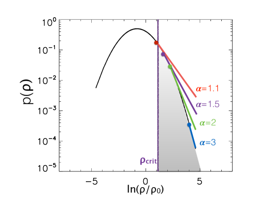
Figure 1.— A cartoon of the density/column density PDF in and around star forming molecular clouds which consists of a lognormal distribution at low density and a power law distribution at high density. As dense material collapses, the power law slope ($\alpha$) becomes shallower and the transition point between the lognormal and power law moves towards lower density values, as indicated with different colored slopes and transition density points. The $SFR_{ff}$ is calculated as an integral over densities greater than $\rho_{crit}$, as indicated in the shaded gray box for the black lognormal PDF.

2. Review of The Star Formation Rate based on Lognormal Density PDFs

A number of past studies have developed an analytic derivation of the SFR based on the statistics of supersonic magnetized turbulence (Krumholz & McKee, 2005; Padoan & Nordlund, 2011; Hennebelle & Chabrier, 2011; Federrath & Klessen, 2012). All of these models take an integral over the lognormal density PDF (Equation 2) in order to estimate the gas mass above a given density threshold that forms stars. Here we briefly review the basic points of these works, namely how the SFR is derived from the lognormal PDF and its dependencies on the properties of turbulence. We note that many other LN SFR models exist in the literature but we focus our comparison on a subset of them as the basic features are similar. The methodology outline in this section will be repeated for the LN+PL density PDF model derived in this work.

The analytic models of Krumholz & McKee (2005), Padoan & Nordlund (2011), and Hennebelle & Chabrier (2011) for the SFR per free-fall ($\mathrm{SFR}_{\mathrm{ff}}$) integrate the lognormal density PDF, Equation (2) multiplied by $\rho/\rho_{0}$ and a normalized free fall factor. This then provides the star formation rate per free-fall time ($\mathrm{SFR}_{\mathrm{ff}}$), first described in Krumholz & McKee (2005), which is the mass fraction going into stars per free-fall time:

$$\rm{SFR_{ff}}={\epsilon_{0}}{\int}_{s_{\mathrm{crit}}}^{\infty}{\frac{t_{\mathrm{ff}}(\rho_{0})}{t_{\mathrm{ff}}(\rho)}\frac{\rho}{\rho_{0}}\,p_{LN}(s)\,\mathrm{d}s}\,.$$ (7)

where $\epsilon_{0}$ is the local efficiency for converting gas into stars and depends on the properties of feedback and $s_{\rm{crit}}=\rm{ln}(\rho_{crit}/\rho_{0})$ is the critical density for collapse. Given the SFR per free-fall time one can also calculate the SFR:

$$SFR=\frac{M_{\rm{cloud}}}{t_{\rm{ff}}(\rho_{0})}SFR_{ff}.$$ (8)

There are two main distinction between different LN SFR models: the free fall factor used, i.e. the treatment of the $\frac{t_{\mathrm{ff}}(\rho_{0})}{t_{\mathrm{ff}}(\rho)}$ term in Equation 7, and the definition of the critical density ($s_{\rm{crit}}$). Krumholz & McKee (2005) estimate the $\mathrm{SFR}_{\mathrm{ff}}$ with a factor $t_{\mathrm{ff}}(\rho_{0})/t_{\mathrm{ff}}(\rho_{0})=1$ while Padoan & Nordlund (2011) uses a factor $t_{\mathrm{ff}}(\rho_{0})/t_{\mathrm{ff}}(\rho_{\mathrm{crit}})$. Both of these studies use a free fall factor which is independent of density and can therefore be taken out of the integral. $t_{\mathrm{ff}}(\rho_{0})/t_{\mathrm{ff}}(\rho)$ appears inside the integral in studies by Hennebelle & Chabrier (2011) and Federrath & Klessen (2012) because gas with different densities has different free-fall times. These studies are therefore termed “multi-free fall” SFR models. As for the differences in the critical density, we summarize the different critical densities and corresponding SFR_ff for the models that employ a LN density PDF (see also Table 1 of Federrath & Klessen (2012)) .

• Krumholz & McKee (2005):

  The critical density for Equation 7 for the Krumholz & Mckee (2005, KM) model is their Equation 27:

  $$\rho_{\rm{crit,KM}}/\rho_{0}=\frac{\pi^{2}}{15}\phi_{t}^{2}\alpha_{\mathrm{vir}}M_{s}^{2}$$ (9)

  where $\alpha_{\mathrm{vir}}$ is the virial parameter, $\phi_{t}$ is of order unity and accounts for the uncertainty in the timescale factor originally introduced in Krumholz & McKee (2005), and $M_{s}$ is the sonic Mach number. The corresponding SFR_ff with $t_{\mathrm{ff}}(\rho_{0})/t_{\mathrm{ff}}(\rho_{0})=1$ is:

  $$SFR_{\rm{ff,KM}}=\frac{\epsilon_{0}}{2\phi_{t}}\left\{1+\mathrm{erf}\left[\frac{\sigma_{s}^{2}-2s_{\mathrm{crit}}}{2\sqrt{2}\sigma_{s}}\right]\right\}$$ (10)

• Padoan & Nordlund (2011):

  The critical density for Equation 7 for the Padoan & Nordlund (2011, PN) model is their Equation 18:

  $$\rho_{crit,PN}/\rho_{0}=0.067\theta^{-2}\alpha_{\mathrm{vir}}M_{s}^{2}f(\beta)$$ (11)

  where $\theta\approx 0.35$ is the ratio of the cloud size over the turbulent integral scale. The PN critical density therefore has the same proportionality with sonic Mach number and virial parameter as the KM model. The effect of the magnetic field in slowing down star formation is encompassed in the function with dependency on plasma Beta ($\beta$, the ratio of thermal to magnetic pressure):

  $$f(\beta)\equiv\frac{\left(1+0.925\beta^{-3/2}\right)^{2/3}}{\left(1+\beta^{-1}\right)^{2}}$$ (12)

  and the corresponding SFR_ff with $t_{\mathrm{ff}}(\rho_{0})/t_{\mathrm{ff}}(\rho_{\mathrm{crit}})$ pulled out of the integral in Equation 7 is:

  $$SFR_{\rm{ff,PN}}=\frac{\epsilon_{0}}{2}\left\{1+\mathrm{erf}\left[\frac{\sigma_{s}^{2}-2s_{\mathrm{crit}}}{2\sqrt{2}\sigma_{s}}\right]\right\}\exp\left(s_{\mathrm{crit}}/2\right)$$ (13)

  The form of SFR_ff in Padoan & Nordlund (2011) therefore nearly identical the SFR in KM but multiplied by an additional exponential term which arises from including $t_{\mathrm{ff}}(\rho_{0})/t_{\mathrm{ff}}(\rho)=t_{\mathrm{ff}}(\rho_{0})/t_{\mathrm{ff}}(\rho_{\mathrm{crit}})$. In both cases $\rho_{crit}\propto\alpha_{vir}M_{s}^{2}$.

• Hennebelle & Chabrier (2011) & (Federrath & Klessen, 2012):

  The critical density for Equation 7 for the Hennebelle & Chabrier (2011,HC) is specified in follow-up papers by Federrath & Klessen (2012) and Hennebelle & Chabrier (2013). In the HC model, the critical density is defined by requiring that the turbulent Jeans length at the critical density is a fraction (which they denote as $ycut$) of the cloud size scale. This is in contrast to the KM and PN models in which the critical density is proportional to ${M_{s}}^{2}$, implying that only very dense structures will lead to star formation. In the HC definition, any structure can collapse if its gravitational energy dominates over all sources of support (thermal, turbulent and magnetic), as long as the associated perturbation can grow and become unstable.

  $$s_{\mathrm{crit}}{{}_{\mathrm{,HC}}}=\ln{\left[\rho_{\mathrm{crit,th}}/\rho_{0}+\rho_{\mathrm{crit,turb}}/\rho_{0}\right]}\,,$$ (14)

  where the (magneto)thermal contribution is

  $$\rho_{\mathrm{crit,th}}/\rho_{0}\equiv\frac{\pi^{2}}{5}y_{\mathrm{cut}}^{-2}\alpha_{\mathrm{vir}}M_{s}^{-2}(1+\beta^{-1})\,,$$ (15)

  and the turbulent contribution is

  $$\rho_{\mathrm{crit,turb}}/\rho_{0}\equiv\frac{\pi^{2}}{15}\,y_{\mathrm{cut}}^{-1}\,\alpha_{\mathrm{vir}}\,.$$ (16)

  The HC model keeps the factor of $t_{\mathrm{ff}}(\rho_{0})/t_{\mathrm{ff}}(\rho)$ inside the integral. The SFR_ff,HC as reviewed in (Federrath & Klessen, 2012) is their Equation 40:

  $$SFR_{\rm{ff,HC}}=\frac{\epsilon_{0}}{2\phi_{t}}\left\{1+\mathrm{erf}\left[\frac{\sigma_{s}^{2}-s_{\mathrm{crit}}}{\sqrt{2}\sigma_{s}}\right]\right\}\exp\left[(3/8)\sigma_{s}^{2}\right]$$ (17)

  We note that the multi-free-fall SFR_ff extension discussed in Federrath & Klessen (2012) for the Krumholz & McKee (2005) and Padoan & Nordlund (2011) models has the same form as Equation 17.

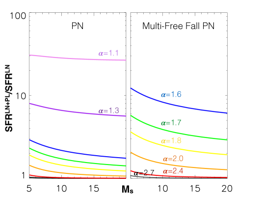
Figure 2.— A comparison of the SFR_ff for a piecewise lognormal and power law (LN+PL) density PDF and a lognormal (LN) density PDF (based on the critical density formula of Padoan & Nordlund (2011)). We plot the ratio of $SFR_{ff}^{LN+PL}$/$SFR_{ff}^{LN}$ vs. the sonic Mach number for b=0.4 (a mix of solenoidal and compressive forcing) and allow the slope of the power law tail ($\alpha$) to vary (shown with different colored lines). Left panel: calculations done with the free-fall factor pulled out of the integral, i.e., Equations 13 vs. 27. Right panel: calculations are multi-free-fall, Equations 17 vs. 28. For $\alpha<2$ the LN+PL models show enhanced star formation rates over the pure lognormal calculations.

3. The Piecewise Lognormal + Power Law Density PDF

The analytic models for the SFR rate of Krumholz & McKee (2005),  Padoan & Nordlund (2011), and Hennebelle & Chabrier (2011), as well as follow-up modifications discussed by Federrath & Klessen (2012), Federrath & Banerjee (2015b), and Gribel et al. (2017), are all based on integrals over the lognormal density PDF thereby neglect contributions to the SFR that arise from the PDF power law tail. Numerous studies have now shown that the lognormal form of the PDF of column density or density describes the behavior of diffuse molecular and atomic gas (Berkhuijsen & Fletcher, 2008; Hill et al., 2008; Burkhart et al., 2010; Imara & Burkhart, 2016; Bialy et al., 2017a). However, as reviewed in the introduction, the dense star-forming gas PDF predominantly takes a piecewise lognormal plus power law form in both 3D density (from simulations) and column density tracers (Kainulainen et al., 2009; Collins et al., 2012; Burkhart et al., 2015a, b; Schneider et al., 2015a; Burkhart et al., 2015b; Imara & Burkhart, 2016). In some cases the PDF of GMCs may be fully power law (Lombardi et al., 2015; Alves et al., 2017).

In light of these studies, we now consider the SFR calculation for a piecewise form of the density PDF in and around a star forming molecular cloud that consists of a lognormal at low density, a power law at high density and a transition point ($s_{t}=ln(\rho_{t}/\rho_{0})$) between the two. This form of the PDF was considered in recent works such as Collins et al. (2012) and Burkhart et al. (2017):

$$p_{LN+PL}(s)=\begin{cases}N\frac{1}{\sqrt{2\pi}\sigma_{s}}e^{\frac{(s-s_{0})^{2}}{2\sigma_{s}^{2}}},&s<s_{t}\\ NCe^{-\alpha s},&s>s_{t},\end{cases}$$ (18)

where again, $s_{0}=-\frac{1}{2}\,\sigma_{s}^{2}$

Here the normalization $N$ is determined by the normalization requirement: $N\int_{-\infty}^{\infty}p_{LN+PL}(s)ds=1$, and is given by

$$N=\left(\frac{Ce^{-\alpha s_{t}}}{\alpha}+\frac{1}{2}{+\frac{1}{2}\rm erf}\left(\frac{2s_{t}+\sigma_{s}^{2}}{2\sqrt{2}\sigma_{s}}\right)\right)^{-1}$$ (19)

We note that in our definition of the power law slope $\alpha$ is positive since the minus sign appears in the exponent separately. Assuming that $p_{LN+PL}(s)$ is continuous and differentiable we can formulate an analytic estimate for $C$ and $\mathrm{s}_{t}$. These two conditions yield:

$$s_{t} =(\alpha-1/2)\sigma_{s}^{2}$$ (20)

And the amplitude of the powerlaw:

$$C=\frac{e^{1/2(\alpha-1)\alpha\sigma_{s}^{2}}}{\sigma_{s}\sqrt{2\pi}}$$ (21)

The transition density value between the lognormal and power law PDFs therefore depends on the slope of the power law, the width of the lognormal and the mean density since $s_{t}=ln(\rho/\rho_{0})$.

We pause here to discuss the physical meaning of the power law slope in the context of the piecewise PDF and the transition density. Numerical simulations of gravoturbulence suggest that the PDF of non-collapsing regions retrain the characteristics of the initial supersonic turbulence field (e.g. remain in the lognormal) while the density PDFs of collapsing regions show a clear power law at high density (Collins et al., 2012; Lee et al., 2015; Mocz et al., 2017). Once the critical density for gravitational collapse is reached the power law begins to form. The characteristic slope of that power law changes in roughly the cloud mean free fall time from steep, $\alpha\approx 3$, to shallow values, $\alpha\approx$1.5 to 1 (Girichidis et al., 2014; Burkhart et al., 2017). The exact time scale for $\alpha$ to saturate depends on the strength of the magnetic field (Burkhart et al., 2015a). The saturation value for the power law slope can be analytically determined from scale-free gravitational collapse (Girichidis et al., 2014; Guszejnov et al., 2017). As $\alpha$ shallows, the transition density ($s_{t}$ between the PDF lognormal and power law moves towards lower density (Equation 20). We illustrate the change of the power law slope and transitional density in Figure 1.

By combining Equation 20 and Equation 5, the transition point can be further related to the physics of the medium (Burkhart et al., 2017):

$$s_{t}=\frac{1}{2}(2\alpha-1)\ln[1+b^{2}M_{s}^{2}]$$ (22)

The PDF transition density can then be expressed in terms of the isothermal post-shock density, $\rho_{\rm{ps}}=\rho_{0}M_{s}^{2}$, which is the density at which the turbulent energy density is equal to the thermal pressure:

$$1/2\rho_{\rm{ps}}c_{s}^{2}=1/2\rho_{0}v^{2}.$$ (23)

Manipulating this relation we find that $M_{s}^{2}=\rho_{\rm{ps}}/\rho_{0}$, and Equation 22 becomes

$$s_{t}=(\alpha-1/2)\ln[1+b^{2}\frac{\rho_{\rm{ps}}}{\rho_{0}}].$$ (24)

In the limit of strong collapse, $\alpha$ tends to 1.5 (Girichidis et al., 2014) and therefore the $(\alpha-1/2)$ term is of order unity.

Therefore,

$$\rho_{t}/\rho_{0}\approx\left(1+b^{2}\frac{\rho_{\rm{ps}}}{\rho_{0}}\right).$$ (25)

For $\alpha=-1.5$ Equation 25 provides a direct physical interpretation for the PDF transition density in terms of the driving of the turbulence ($b$) and the post-shock density: $s_{t}(\alpha=1.5)=\sigma_{s}^{2}$. The transition density is proportional to the critical density for collapse based on the post-shock density derived in Krumholz & McKee (2005) and Padoan & Nordlund (2011). We will explore the relationship between the transition density and the critical density for collapse in companion papers: Burkhart & Mocz (2018) and Mocz & Burkhart (2018).

4. The Dynamic Star Formation Rate in the Gravoturbulent Media

Given the analytic expressions for the normalization constants and transition density point (Equations 19-22), we can now integrate the piecewise density PDF and predict the star formation rate.

In what follows, we consider the original formulation for the critical density for collapse $\rho_{crit}$ as defined in Padoan & Nordlund (2011) in Equation 11 with $\alpha_{\mathrm{vir}}=1$, a weak magnetic field ($\beta=20$), and ratio of cloud size to turbulence integral scale of $\theta=0.35$. In general, this is similar to the formulation of Krumholz & McKee (2005): $\rho_{crit,KM}/\rho_{0}=(\pi^{2}/15)\phi_{t}^{2}\times\alpha_{\mathrm{vir}}M_{s}^{2}$, where $\alpha_{\mathrm{vir}}=\phi_{t}=1$. We also consider the multi-free-fall piecewise density PDF SFR calculation derived in Federrath & Klessen (2012), again using the critical density of Padoan & Nordlund (2011) in Equation 11. We plan to explore the full parameter space of $\alpha_{\mathrm{vir}}$, $\beta$ and choice of critical density elsewhere.

The integral to calculate the SFR_ff now splits into an integral over the lognormal from $\rho_{crit}$ to $\rho_{t}$ and an integral over the power law from $\rho_{t}$ to infinity:

$$SFR_{ff}^{LN+PL}=\epsilon_{0}{\int}_{s_{\mathrm{crit}}}^{\mathrm{s}_{t}}{\frac{t_{\mathrm{ff}}(\rho_{0})}{t_{\mathrm{ff}}(\rho)}\frac{\rho}{\rho_{0}}\,p(s)_{LN}\,\mathrm{d}s}~{}$$

$$+\epsilon_{0}{\int}_{\mathrm{s}_{t}}^{\infty}{\frac{t_{\mathrm{ff}}(\rho_{0})}{t_{\mathrm{ff}}(\rho)}\frac{\rho}{\rho_{0}}\,p(s)_{PL}\,\mathrm{d}s}\,.$$ (26)

If we consider the free-fall factor weighting to be a constant $t_{\mathrm{ff}}(\rho_{0})/t_{\mathrm{ff}}(\rho_{crit})$, and pull it out of the integral, then Equation 26 evaluates to:

$$SFR_{ff}^{LN+PL} ={\rm{exp}(s_{\mathrm{crit}}/2)}N\epsilon_{0}\bigg{[}\frac{1}{2}\mathrm{erf}\left(\frac{\sigma_{s}^{2}-2s_{\mathrm{crit}}}{\sqrt{8\sigma_{s}^{2}}}\right)$$

$$-\frac{1}{2}\mathrm{erf}\left(\frac{\sigma_{s}^{2}-2s_{t}}{\sqrt{8\sigma_{s}^{2}}}\right)+C\frac{\rm{exp}(s_{t}(1-\alpha))}{\alpha-1}\bigg{]}$$ (27)

which is limited to $\alpha>1.0$ If the free fall factor is unity than the factor of ${\rm{exp}(s_{\mathrm{crit}}/2)}$ is removed.

When the free-fall factor is kept inside the integral, the LN+PL star formation rate per free-fall time becomes:

$$SFR_{\rm{multiff}}^{LN+PL}=\frac{\rm{exp}(3\sigma_{s}^{2}/8)N\epsilon_{0}}{2}\bigg{[}\mathrm{erf}\left(\frac{\sigma_{s}^{2}-s_{\mathrm{crit}}}{\sqrt{2\sigma_{s}^{2}}}\right)$$

$$-\mathrm{erf}\left(\frac{\sigma_{s}^{2}-s_{t}}{\sqrt{2\sigma_{s}^{2}}}\right)\bigg{]}+N\epsilon_{0}\left[C\frac{\rm{exp}(s_{t}(1.5-\alpha))}{\alpha-1.5}\right]$$ (28)

which is limited to $\alpha>1.5$

The SFR can be calculated according to Equation 8. As shown in Figure 1, when $\alpha$ is steep, the density transition point is larger and hence the power law portion contributes very little to the $\mathrm{SFR}_{\mathrm{ff}}$. The power-law tail appears first at high densities and steadily extends to lower densities as time proceeds, which has been shown analytically (Girichidis et al., 2014) and numerically (Collins et al., 2012; Burkhart et al., 2015a, 2017). Equation the $\mathrm{SFR}_{\mathrm{ff}}$ depends increasingly on the power law portion of the piecewise PDF as $\alpha$ become shallower.

In Figure 2 we compare the $SFR_{ff}$ vs. sonic Mach number for a pure lognormal SFR_ff (Equation 13) to the LN+PL $SFR_{ff}$ calculation. The left panel compares the original derivation from Padoan & Nordlund (2011) to Equation 27, while the right panel compares the multi-free-fall expression derived in Federrath & Klessen (2012), Equation 17 to the LN+PL multi-free-fall expression in Equation 28.

We chose $b=0.4$ (a mix of solenoidal and compressive forcing) and allow the sonic Mach number (x-axis) and $\alpha$ to vary. Different colored lines in Figure 2 indicate different values of $\alpha$. For steep values of the power law tail slope, the $SFR_{ff}^{LN+PL}$ is very similar to the lognormal expression ($SFR_{ff}^{LN}$). However, as $\alpha$ becomes increasingly shallow the star formation rate can grow to more than an order of magnitude above the pure lognormal calculation for both the multi-free-fall expression as well as the expression with the free-fall factor pulled out of the integrals.

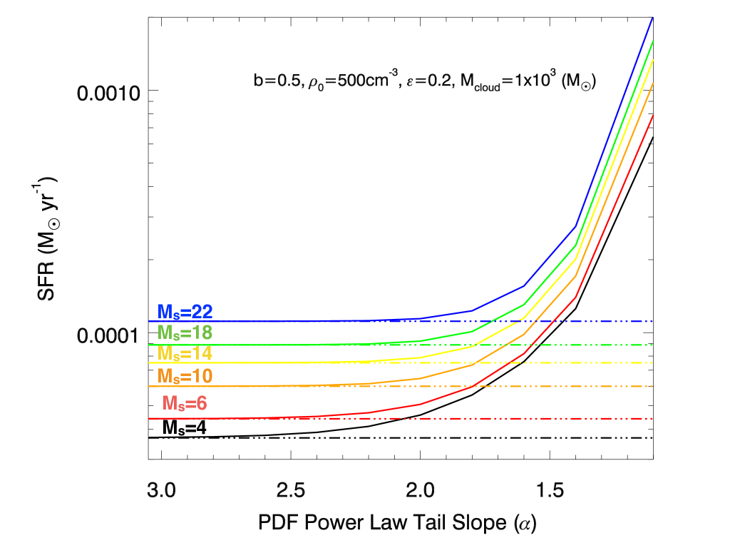
Figure 3.— Analytic calculations for the star formation rate per free fall time (SFR_ff) vs. the density PDF power law slope ($\alpha$). The top panel using the free fall factor of (Padoan & Nordlund, 2011). Solid lines are for the SFR calculated using the lognormal+power law (LN+PL) model (Equation 27) and the straight dashed-dotted lines are for the pure lognormal (LN) models (Equation 13). The bottom panel shows the same but uses the free fall factor of (Krumholz & McKee, 2005), e.g. the factor of exp$(s_{crit}/2)$ is removed. For both the top and bottom panel, the critical density used is the same (Equation 11). Different colored lines indicate changing the sonic Mach number, with black representing the smallest value considered ($M_{s}=4$) and blue representing the largest value considered ($M_{s}=22$). The LN only SFR calculation only depends on the properties of the turbulence (sonic Mach number and forcing parameter $b$) and hence has no dependency on $\alpha$. Regardless of the free fall factor used, as $\alpha$ becomes increasingly shallow, the PL+LN model presented here begins to diverge from the LN model, with differences in the sonic Mach number becoming less significant.

Figure 2 also predicts that, when a time variable power law is included, the star formation rate is not constant. This is in contrast to the lognormal theories reviewed in Section 2 that are constant with the properties of MHD turbulence, which set the width of the lognormal, e.g., Equation 5.

Figure 3 shows the star formation rate per free fall time (SFR_ff) vs. the density PDF power law slope ($\alpha$) for both the LN+PL (Equation 27) and LN models. In the top panel, we compare the $SFR_{ff}^{LN}$ expression of Padoan & Nordlund (2011), Equation 13, with the $SFR_{ff}^{LN+PL}$ shown in Equation 27. The bottom panel shows the same comparison but using a free fall factor of unity as prescribed in Krumholz & McKee (2005) (Equation 10). In both panels, the LN SFR calculation only depends on the properties of the turbulence (sonic Mach number and forcing parameter $b$) and has no dependency on $\alpha$. When using the Padoan & Nordlund (2011) free fall factor (top panel), the SFR_ff for both LN and LN+PL models increases with increasing sonic Mach number (i.e. increasing PDF width).

The primary difference between the top and bottom panels stems from the factor of exp$(s_{crit}/2)$, which is present in the Padoan & Nordlund (2011) and absent in the Krumholz & McKee (2005) model due to the different treatment of the free fall factor. As noted in Krumholz & McKee (2005) the combination of critical density increasing as sonic Mach number squared and a free fall factor of unity produces a SFR_ff that is slightly anti-correlated with sonic Mach number, in contrast to the models of Padoan & Nordlund (2011), Hennebelle & Chabrier (2011), and Federrath & Klessen (2012). The Mach number dependency is also shown in Figure 1 of Federrath & Klessen (2012). This demonstrates that different treatments of the free fall factor become important in both the LN and LN+PL models and can produce more than an order of magnitude difference in the value of SFR_ff.

As $\alpha$ becomes increasingly shallow, the LN+PL models begin to diverge from the LN models. The width of the lognormal portion of the PDF sets the value of $\alpha$ for which the two models diverge. Lower values of $M_{s}$ show divergence at earlier stages of cloud evolution, i.e. steeper values of $\alpha$, regardless of the free fall factor criterion used. The models begin to diverge strongly around $\alpha=2$.

5. Comparison With Observations

In what follows, we compare the star formation rate using the LN+PL density PDF to observations of local GMCs. We also investigate how our model can predict the slope and scatter of the relationship between the mass of molecular gas and the star formation rate (Gao & Solomon, 2004; Lada et al., 2010; Heiderman et al., 2010; Lada et al., 2012; Faesi et al., 2014).

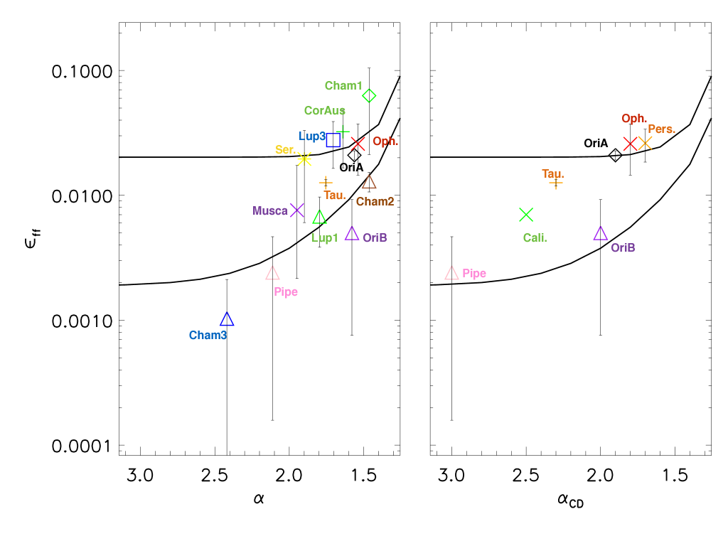
Figure 4.— The star formation efficiency per free fall ($\epsilon_{ff}$) vs. the slope of the density PDF power law (left panel) and column density PDF power law slope (right panel). The local GMC values for the PDF slopes, $<\epsilon_{ff}>$ and the references used are given in Table 1. Local GMCs are represented by colored points and the LN+PL model predictions are shown in black lines bounding the parameter space of b=0.3-0.7 and M${}_{s}=5-25$.

5.1. Local Giant Molecular Clouds and the Star Formation Efficiency

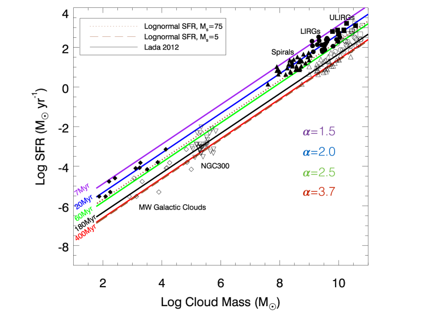
Figure 5.— The SFR vs. cloud mass relationship, with the solid black line showing the relation from Lada et al. (2012). Lada et al. (2010, 2012) published values of local GMCs (diamonds), spiral galaxies (upward triangles), Luminous Infrared Galaxies (LIRGS, circles), and Ultra-luminous Infrared Galaxies (ULIRG, squares). Individual GMCs from NGC 300 were published in Faesi et al. (2014) (downward triangles). Open symbols correspond to diffuse gas tracers (either dust extinction at 0.1 mag or CO) while closed symbols indicate dense gas tracers (either dust extinction at 0.8 mag or HCN). Rainbow colored solid lines are different LN+PL model predictions for the SFR with $M_{s}=5,b=1/3$ and different values of $\alpha$, which can greatly change the amplitude of the SFR and hence contribute to the scatter in SFR despite the constant turbulence properties. For each of the LN+PL models we over-plot the corresponding depletion times. Two lognormal only models are shown in brown dotted ($M_{s}=75,b=1/3$) and dashed lines ($M_{s}=5,b=1/3$) can only explain the scatter if they have extreme variations in turbulence parameters or the ad-hoc SFE parameter.

A number of observational studies have been conducted to understand the relationship between the dense gas mass fraction, the gas density PDF and the properties of star formation such as the star formation efficiency per free fall time ($\epsilon_{ff}$). We define $\epsilon_{ff}$ as in Krumholz & McKee (2005):

$$\epsilon_{ff}=SFR\frac{t_{ff}(\rho_{0})}{M_{\rm{cloud}}}$$ (29)

Examples of such studies include Lada et al. (2010), Heiderman et al. (2010) and Kainulainen et al. (2014), who investigated the level of star formation activity and cloud structure in nearby GMCs. Krumholz et al. (2012) summarized the observed data from Lada et al. (2010) and Heiderman et al. (2010) and derived the star formation efficiency per free fall time (see their Table 2). For many of the clouds studied in Lada et al. (2010), Lombardi et al. (2015) also calculated the slope of their column density PDF power law ($\alpha_{CD}$) using dust extinction/emission data from Planck, Herschel and 2MASS. Burkhart et al. (2015a) also noted that there is a correlation in local GMCs with shallower column density power law tails and an increase in the number of young stellar objects (NYSO), which is proportional to the SFR. More recently, Kainulainen et al. (2014) derived 3D density GMC PDFs for 16 clouds using a wavelet-based reconstruction technique. The reported cloud masses, cloud densities, and NYSO, all of which can be used to derive the SFRs and SFEs. Kainulainen et al. (2014) also measured the exponent of the radial density distribution ($\kappa$), which is related to the PDF density slope as $\kappa=3/\alpha$. We compile values of $\alpha$, $\alpha_{CD}$ and the average value of $\epsilon_{ff}$ from the above mentioned studies and present them in Table 1.

Table 1GMC star formation efficiency per free fall time, references: ¹Kainulainen et al. (2014),²Lada et al. (2010), ³Heiderman et al. (2010),⁴Krumholz et al. (2012),⁵Lombardi et al. (2015)

GMC	$<\epsilon_{ff}>$	$\alpha_{CD}$	$\alpha$	Ref.
Orion A	0.021	1.9	1.56	1,2,4,5
Orion B	0.005	2	1.58	1,2,4,5
Oph.	0.026	1.8	1.54	1,2,3,4,5
Taurus	0.013	2.3	1.75	1,2,4,5
Serpens	0.017	N/A	1.9	1,3,4
ChamI	0.06	N/A	1.46	1,3,4
ChamII	0.013	N/A	1.46	1,3,4
LupI	0.007	N/A	1.8	1,2,3,4
LupIII	0.028	N/A	1.7	1,2,3,4
CorA	0.032	N/A	1.64	1,2,3,4
Pipe	0.002	3	2.11	1,2,4,5
Musca	0.008	N/A	1.95	1,3,4
ChaIII	0.001	N/A	2.42	1,3,4
Perseus	0.026	1.7	N/A	2,3,4,5
Cali.	0.0065	2.5	N/A	2,4,5

We plot $\epsilon_{ff}$ vs. power law slope in Figure 4. Error bars on the observations are computed from the standard deviation of the different reported values of $\epsilon_{ff}$ in the literature. The left panel shows $\epsilon_{ff}$ vs. the 3D density $\alpha$ reported in Kainulainen et al. (2014) for local GMCs. The right panel presents $\epsilon_{ff}$ vs. the column density PDF slopes published in Lombardi et al. (2015). For both density and column density PDF power law slopes we note a clear trend of rising $\epsilon_{ff}$ with shallower power law tail slope in the observations. This trend is within the expectations of the LN+PL model (black lines) range for sonic Mach numbers of 5-25 and $b$ values of $1/3-0.7$, although we emphasize that the amplitude depends primarily on the feedback parameter ($\epsilon_{0}$) and which version of the free fall factor is employed. Regardless of these, the rise with shallower $\alpha$ is expected from the model and observed in the local GMCs.

We confirm that there are line of sight effects that may produce a difference between the actual density PDF $\alpha$ and the measured column density PDF $\alpha_{CD}$. These LOS effects may also apply to the reconstructed density power law slope measured in Kainulainen et al. (2014). Burkhart et al. (2015a) and Burkhart et al. (2017) studied the column density PDF properties and compared them to the density PDF properties from Collins et al. (2012). They found that for the same time step and plasma $\beta$ (mean magnetic field strength) the power law slopes of column density PDF can change slightly depending on the LOS orientation. Girichidis et al. (2014) and Guszejnov et al. (2017) performed analytic calculations for the evolution of the power-law PDF slopes for both density and column density of all material which undergoes complete fragmentation (e.g. goes on to form stars). In particular, the results of Guszejnov et al. (2017) suggest that the density and column density power law slopes should converge to values of -1. However, they argue that the column density PDF is affected by LOS effects which steepens the slope, most likely producing final slopes roughly between -1 and -2. Indeed for all the clouds examined here $\alpha_{CD}>\alpha$. Additional studies comparing the analytic results of Girichidis et al. (2014) and Guszejnov et al. (2017) to numerical simulations will be useful to determine the correspondence between column density PDF $\alpha_{CD}$ and the density PDF $\alpha$.

Despite the observational complications of measuring $\epsilon_{ff}$ and the PDF properties (Alves et al., 2017), a very clear trend of increasing $\epsilon_{ff}$ with shallower $\alpha$ is seen for the local GMCs. An important distinction between the analytic SFR model derived in this work and the works of Krumholz & McKee (2005), Padoan & Nordlund (2011) and Hennebelle & Chabrier (2011) is that they provide a constant $SFR_{ff}$ and/or $\epsilon_{ff}$ for given turbulence parameters, such as the sonic Mach number and the forcing, which set the lognormal width. However, it is not likely that differences in $\epsilon_{ff}$ observed in the data is due the properties of turbulence, as most of these clouds have similar sonic Mach numbers and similar line width size relations (Kainulainen & Federrath, 2017). The LN+PL model $SFR_{ff}$ calculation presented here is inherently time varying as the slope of the power law varies with cloud evolution due to gravitational collapse and feedback. The level of turbulence is secondary to the $SFR_{ff}$ when the power law is taken into account (see Figure 3).

5.2. From Galactic to Extragalactic: Dense Gas Mass and the Star Formation Rate

A number of insightful observational surveys have shed light on the relationship between ISM properties and extragalactic SFR scaling laws. Gao & Solomon (2004) found a linear relation between the SFR traced by total infrared luminosity and the luminosity in a dense gas tracer (HCN) averaged over entire galaxies (see also, Wu et al. (2005)). Similar relations between dense gas mass or gas surface density and star formation rates have been observed in a number of recent extragalactic surveys (Bigiel et al., 2008; Schinnerer et al., 2013; Pety et al., 2013; Hughes et al., 2013; Colombo et al., 2014; Faesi et al., 2014; Usero et al., 2015a; Bigiel et al., 2016; Leroy et al., 2017; Federrath et al., 2017) as well as in local well-resolved Milky Way GMCs (Heiderman et al., 2010; Lada et al., 2010)

The relationship between molecular gas mass and the SFR was further extended in Lada et al. (2012) and Faesi et al. (2014), who showed that the same linear correlation smoothly extends across more than five orders of magnitude when connected to local galaxy dense gas masses and star formation rates and is consistent with the Gao & Solomon (2004) and Wu et al. (2005) results to within a factor of three. One interpretation of this linear slope is an approximately constant depletion time ($\rm{t_{\rm{depl}}(yr)=M_{\rm{mol}}(M_{\odot})/SFR(M_{\odot}/yr)}$), i.e., the timescale for the molecular gas to be converted into stars. Extragalactic studies consistently derive average depletion times of about 2 Gyr (Bigiel et al., 2008; Leroy et al., 2013b, a), however deviations have been noted (Leroy et al., 2011; Saintonge et al., 2011a, b; Sandstrom et al., 2013; Burkert & Hartmann, 2013). These deviations could be due to systematics and/or true environmental differences in galaxies. Furthermore, local MW GMCs and resoled GMCs in nearby galaxies have a median $t_{\rm{depl}}$ of 180-230 Myrs, an order of magnitude shorter than the typical values found in unresolved extragalactic studies (Lada et al., 2010, 2012; Faesi et al., 2014). Dense gas tracers have even shorter depletion times of around 20 Myrs (Lada et al., 2012).

We explore these trends using the predictions of LN+PL SFR model and compare with the LN only model. Figure 5 shows the SFR vs. cloud mass for local GMCs and galaxies, with the solid black line showing the fit from Lada et al. (2012) and data from (Gao & Solomon, 2004). Lada et al. (2010, 2012) published values of local GMCs (diamonds), spiral galaxies (upward triangles), Luminous Infrared Galaxies (LIRGS, circles), and Ultra-luminous Infrared Galaxies (ULIRG, squares). GMCs from NGC 300 were published in Faesi et al. (2014) (downward triangles). Opened symbols correspond to diffuse gas tracers (either dust extinction at 0.1 mag or CO) while closed symbols indicate dense gas tracer (either dust extinction at 0.8 mag or HCN). Rainbow colored solid lines are different LN+PL model predictions for the SFR with $M_{s}=5,b=1/3$ and different values of $\alpha$, which can greatly change the amplitude of the SFR and hence contribute to the scatter in SFR despite the constant turbulence properties. For each of the LN+PL models we over-plot the corresponding depletion times. Two lognormal only models are shown in brown dotted ($M_{s}=75,b=1/3$) and dashed lines ($M_{s}=5,b=1/3$).

The lognormal and steep LN+PL models (red, orange and yellow lines) show agreement with observations of diffuse molecular gas tracers (open symbols). These tracers are more likely to lie within the lognormal portion of the gas PDF since they are diffuse. However the high density gas tracers (e.g. HCN, filled symbols) show better correspondence with shallower power law slope values of the SFR (green, blue and purple lines). The LN SFR models could explain these points as well but only for extreme sonic Mach numbers in the range of $M_{s}=75-100$ (Federrath, 2013b; Usero et al., 2015a; Federrath et al., 2017) or invoking large variations in the star formation efficiency. Typical sonic Mach numbers measured in local star forming Milky Way clouds lie in the range of $M_{\rm{s,MilkyWay}}=4-20$, (Burkhart et al., 2010; Kainulainen & Tan, 2013; Kainulainen & Federrath, 2017).

As seen in the previous section in Figure 2, the LN+PL model SFR can change by more than an order of magnitude for different values of $\alpha$ and hence can explain the scatter in the SFR with the average observed Mach numbers in the ISM. A shallower value of $\alpha$ corresponds to increasing the fraction of dense gas (f_dense), which is representative of star formation law discussed in Lada et al. (2012): SFR $\propto f_{dense}M_{cloud}$.

For each of the three LN+PL models we over-plot the corresponding depletion times, $t_{\rm{depl}}=7,20,60,400$ Myr for $\alpha=1.5,2.0,2.5,3.7$, respectively. Clouds with shallow power law tails have the shortest depletion times, the most dense self-gravitating gas in the power law tail, and rapid star formation, while clouds with steep power law tails or lognormal distributions with moderate sonic Mach numbers have longer depletion times.

The star formation rate and depletion time is primarily controlled by the local dense gas fraction which, in the context of the density PDF SFR model presented here, is characterized by the amount of material in the power law portion of the PDF. Once the critical density is reached, the value of $\alpha$ rapidly shallows and the lognormal portion of the SFR calculation becomes insignificant. Therefore the value of $f_{dense}$, and hence the overall SFR, is determined by the competition of gravity vs. feedback and secondarily on magnetic fields and large scale turbulence.

6. Discussion

The LN+PL model discussed here can be retermed as a gravoturbulent star formation model since the development of lognormal plus power law density distribution is consistent with the picture of a turbulent molecular cloud undergoing gravitational collapse. Both numerical experiments and observations point to a picture of a dynamic star formation rate, which increases in time as clouds become gravitationally unstable (Hartmann et al., 2001; Vázquez-Semadeni et al., 2007; Heitsch et al., 2008; Heitsch & Hartmann, 2008; Hennebelle & Teyssier, 2008; Banerjee et al., 2009; Zamora-Avilés et al., 2012; Burkert & Hartmann, 2013; Girichidis et al., 2014; Zamora-Avilés & Vázquez-Semadeni, 2014) and later halts as feedback/supernova destroy the star forming region. The model presented here, which includes both the lognormal and power law components, is inherently time varying as the power law slope is expected to change as the cloud contracts and later is destroyed by feedback. Previous studies have investigated the SFR or IMF from a power law only distribution with single values of $\alpha$ (Collins et al., 2012; Girichidis et al., 2014; Lee & Hennebelle, 2017). However, GMCs have different observed values of the power law slope and $\alpha$ is expected to become shallow as the cloud evolves from rapidly collapsing filaments (Collins et al., 2012; Federrath & Klessen, 2012; Federrath, 2013b; Schneider et al., 2015b; Burkhart et al., 2015b; Lee et al., 2015; Lee & Hennebelle, 2017; Mocz et al., 2017; Caldwell & Chang, 2018) and the $SFR_{ff}$ increases. $\alpha$ may steepen again as feedback from OB stars destroy the GMC as maybe indicated in GMCs which show multiple power law tail slopes (Schneider et al., 2015a).

As mentioned above, an important distinction between the analytic model presented here and the SFR models of Krumholz & McKee (2005), Padoan & Nordlund (2011) and Hennebelle & Chabrier (2011) is that they provide a constant $SFR_{ff}$ for a given sonic Mach number (i.e. lognormal width), $\beta$, $\alpha_{vir}$ and $\epsilon_{0}$. The model presented here provides the same value of the SFR when the power law tail is very steep and the PDF is dominated by the lognormal. However for clouds with prominent high density power law PDFs the SFR is observed to increase and our model accounts for this effect without the need to invoke stronger turbulence or alternative environmental parameters.

The model presented here suggests that star formation rates and efficiencies are very sensitive to the increasing influence of the gas self-gravity and feedback. The key observable is the manifestation of the power law in the density PDF. In that sense we can explain why observed star formation rates do not show sensitivity or strong correlation with local measurements of velocity dispersion or second moment maps (Leroy et al., 2017) and why star formation correlates strongly with dense gas fraction. We will explore this point further in a follow up paper (Burkhart & Mocz 2018, submitted).

We emphasize that in the analytic formulation for the SFR and SFE outlined in this work there is no need to invoke the ionization state of the cloud or complex plasma processes such as the Hall effect, or ambipolar diffusion. Turbulence, turbulent magnetic fields, and gravity set the basic initial conditions for the star formation rates and efficiencies. Turbulence sets the initial density distribution (i.e. with a lognormal PDF) and can also control the fluctuation, amplification, and diffusion of the magnetic field. A process known as reconnection diffusion (Lazarian & Vishniac, 1999; Lazarian et al., 2012) is mediated by the properties of turbulence. Numerical simulations have shown that magnetic reconnection diffusion can be an important process for mediating collapse (Santos-Lima et al., 2012; Lazarian et al., 2012; Mocz et al., 2017) especially in clouds with sub-Alfvénic and magnetically sub-critical initial conditions (Crutcher et al., 2009b, 2010; Crutcher, 2012). In this paper we only explored a weakly magnetized regime of parameter space with our choice of $\rho_{crit}$ but plan to explore the effects of strong magnetization, where reconnection might play a more important role, in a future work.

The gravoturbulent star formation model has implications for both the Kennicutt-Schmidt relationship as well as the numbers of YSOs in local GMCs. The analytic model outlined here suggests that star formation scaling laws from galaxy scales to cloud scales are driven primarily by variation in the amount of dense gas (set by the power law slope $\alpha$) and secondarily on the properties of turbulence in the clouds. This is in agreement with recent observational work by Lada et al. (2017) on the California GMC as well as work by Elmegreen (2018) on explaining scatter in the Kennicutt-Schmidt relation. The gravoturbulent model can explain the scatter in the SFR vs. dense gas mass observations (Heiderman et al., 2010; Lada et al., 2010, 2012; Faesi et al., 2014; Leroy et al., 2017), without the need to invoke extremely large turbulent energies (e.g. large $M_{s}$). The gravoturbulent model SFR changes by more than an order of magnitude for different values of $\alpha$ and hence could be an explanation for the scatter in the SFR in both local GMCS as well as in extragalactic quiescent vs. starbursting systems. Clouds with shallow power law tails have SFRs dominated by self-gravity and we predict they also have higher dense gas fractions, shorter depletion times and rapid star formation. This is in agreement with the observational studies of Usero et al. (2015b) and Leroy et al. (2017), who found that gas with stronger self-gravity forms stars at a higher rate (lower depletion time). Moreover, these studies found that the star formation efficiency is anti-correlated with the velocity dispersion (Mach number), which is in tension with some lognormal turbulence theories of star formation.

The star formation theory derived in this paper is suitable for application to galaxy/cosmological simulation sub-grid models (Hopkins et al., 2013). Our model predicts that star formation depends primarily on the amount of dense self-gravitating gas and secondarily on the properties of ISM turbulence, which set the initial density fluctuations. Gravitational collapse primarily controls star formation until it is shut of by mass loss and/or feedback processes. Galaxy formation simulations which seek to include ISM physics should adopt a SFR law which has a primary dependency on a dense gas probability and secondarily on the conditions of the ISM including, $\alpha$, $M_{s}$, $\alpha_{vir}$ and $\beta$.

7. Conclusions

Stars form in supersonic turbulent molecular clouds that are self-gravitating. We presented an analytic determination of the star formation rate in a gravoturbulent medium based on the density probability distribution function of molecular clouds having a piecewise lognormal and power law (LN+PL) form. Previous analytic models for the star formation rate based on the density distribution used only the lognormal portion of the PDFs, with properties determined by supersonic turbulence, and ignored the contribution of the high density power law tail set by self-gravity.

In the gravoturblent model presented here, the star formation rate per free-fall time is calculated via an integral over the lognormal from a critical density ($\rho_{crit}$) to the transition density between the lognormal and power law ($\rho_{t}$) and then an integral over the power law from $\rho_{t}$ to infinity. This accounts for clouds which are in the early stages of collapse to later evolutionary stages. The transitional density is analytically determined from the conditions of continuity and differentiability of the PDF (Collins et al., 2012; Burkhart et al., 2017). We find that:

• As the slope of the power law tail becomes shallower the SFR_ff in the gravoturbulent model increases past the expectations of the turbulence SFR models (i.e. pure lognormal PDF models).

• We show that star formation efficiency per free fall time in local giant molecular clouds increases with shallower PDF power law slopes, in agreement with our model.

• The approach presented here can explain why star formation is spatially and temporally variable within a cloud and can accelerate in pace despite roughly constant ISM turbulent energy and magnetic field strengths.

• Clouds with shallow power law tails have a higher dense gas fraction and therefore short depletion times and rapid star formation.

• Our model can explain both star-bursting and quiescent star-forming systems without the need to invoke extreme variations in the local interstellar environment or large sonic Mach numbers.

References

- Agertz et al. (2015) Agertz, O., Romeo, A. B., & Grisdale, K. 2015, MNRAS, 449, 2156
- Alves et al. (2017) Alves, J., Lombardi, M., & Lada, C. J. 2017, A&A, 606, L2
- Ballesteros-Paredes et al. (2011) Ballesteros-Paredes, J., Hartmann, L. W., Vázquez-Semadeni, E., Heitsch, F., & Zamora-Avilés, M. A. 2011, MNRAS, 411, 65
- Banerjee et al. (2009) Banerjee, R., Vázquez-Semadeni, E., Hennebelle, P., & Klessen, R. S. 2009, MNRAS, 398, 1082
- Beaumont et al. (2015) Beaumont, C., Goodman, A., & Greenfield, P. 2015, in Astronomical Society of the Pacific Conference Series, Vol. 495, Astronomical Data Analysis Software an Systems XXIV (ADASS XXIV), ed. A. R. Taylor & E. Rosolowsky, 101
- Berkhuijsen & Fletcher (2008) Berkhuijsen, E. M. & Fletcher, A. 2008, MNRAS, 390, 19
- Bialy et al. (2017a) Bialy, S., Bihr, S., Beuther, H., Henning, T., & Sternberg, A. 2017a, ApJ, 835, 126
- Bialy et al. (2017b) Bialy, S., Burkhart, B., & Sternberg, A. 2017b, ApJ, 843, 92
- Bigiel et al. (2008) Bigiel, F., Leroy, A., Walter, F., Brinks, E., de Blok, W. J. G., Madore, B., & Thornley, M. D. 2008, AJ, 136, 2846
- Bigiel et al. (2016) Bigiel, F., Leroy, A. K., Jiménez-Donaire, M. J., Pety, J., Usero, A., Cormier, D., Bolatto, A., Garcia-Burillo, S., Colombo, D., González-García, M., Hughes, A., Kepley, A. A., Kramer, C., Sandstrom, K., Schinnerer, E., Schruba, A., Schuster, K., Tomicic, N., & Zschaechner, L. 2016, ApJ, 822, L26
- Burkert & Hartmann (2013) Burkert, A. & Hartmann, L. 2013, ApJ, 773, 48
- Burkhart et al. (2015a) Burkhart, B., Collins, D. C., & Lazarian, A. 2015a, ApJ, 808, 48
- Burkhart & Lazarian (2012) Burkhart, B. & Lazarian, A. 2012, ApJ, 755, L19
- Burkhart et al. (2015b) Burkhart, B., Lee, M. Y., Murray, C., & Stanimirovic, S. 2015b, ApJ, 811, 28
- Burkhart et al. (2015c) Burkhart, B., Lee, M.-Y., Murray, C. E., & Stanimirović, S. 2015c, ApJ, 811, L28
- Burkhart et al. (2017) Burkhart, B., Stalpes, K., & Collins, D. C. 2017, ApJ, 834, L1
- Burkhart et al. (2010) Burkhart, B., Stanimirović, S., Lazarian, A., & Kowal, G. 2010, ApJ, 708, 1204
- Caldwell & Chang (2018) Caldwell, S. & Chang, P. 2018, MNRAS, 474, 4818
- Chen et al. (2017) Chen, H., Burkhart, B., Goodman, A. A., & Collins, D. C. 2017, ArXiv e-prints
- Chyba & Hand (2005) Chyba, C. & Hand, K. 2005, Annual Review of Astronomy and Astrophysics, 43, 31
- Collins et al. (2012) Collins, D. C., Kritsuk, A. G., Padoan, P., Li, H., Xu, H., Ustyugov, S. D., & Norman, M. L. 2012, ApJ, 750, 13
- Colombo et al. (2014) Colombo, D., Hughes, A., Schinnerer, E., Meidt, S. E., Leroy, A. K., Pety, J., Dobbs, C. L., García-Burillo, S., Dumas, G., Thompson, T. A., Schuster, K. F., & Kramer, C. 2014, ApJ, 784, 3
- Crutcher (2012) Crutcher, R. M. 2012, ARA&A, 50, 29
- Crutcher et al. (2009a) Crutcher, R. M., Hakobian, N., & Troland, T. H. 2009a, ApJ, 692, 844
- Crutcher et al. (2009b) —. 2009b, ApJ, 692, 844
- Crutcher et al. (2010) Crutcher, R. M., Wandelt, B., Heiles, C., Falgarone, E., & Troland, T. H. 2010, ApJ, 725, 466
- Elmegreen (2018) Elmegreen, B. G. 2018, ArXiv e-prints
- Faesi et al. (2014) Faesi, C. M., Lada, C. J., Forbrich, J., Menten, K. M., & Bouy, H. 2014, ApJ, 789, 81
- Fall et al. (2010) Fall, S. M., Krumholz, M. R., & Matzner, C. D. 2010, ApJ, 710, L142
- Federrath (2013a) Federrath, C. 2013a, MNRAS, 436, 1245
- Federrath (2013b) —. 2013b, MNRAS, 436, 3167
- Federrath & Banerjee (2015a) Federrath, C. & Banerjee, S. 2015a, MNRAS, 448, 3297
- Federrath & Banerjee (2015b) —. 2015b, MNRAS, 448, 3297
- Federrath & Klessen (2012) Federrath, C. & Klessen, R. S. 2012, ApJ, 761, 156
- Federrath et al. (2008) Federrath, C., Klessen, R. S., & Schmidt, W. 2008, ApJ, 688, L79
- Federrath et al. (2017) Federrath, C., Salim, D. M., Medling, A. M., Davies, R. L., Yuan, T., Bian, F., Groves, B. A., Ho, I.-T., Sharp, R., Kewley, L. J., Sweet, S. M., Richards, S. N., Bryant, J. J., Brough, S., Croom, S., Scott, N., Lawrence, J., Konstantopoulos, I., & Goodwin, M. 2017, MNRAS, 468, 3965
- Gao & Solomon (2004) Gao, Y. & Solomon, P. M. 2004, ApJ, 606, 271
- Girichidis et al. (2014) Girichidis, P., Konstandin, L., Whitworth, A. P., & Klessen, R. S. 2014, ApJ, 781, 91
- Goodman et al. (2009) Goodman, A. A., Rosolowsky, E. W., Borkin, M. A., Foster, J. B., Halle, M., Kauffmann, J., & Pineda, J. E. 2009, Nature, 457, 63
- Gribel et al. (2017) Gribel, C., Miranda, O. D., & Williams Vilas-Boas, J. 2017, ApJ, 849, 108
- Guszejnov et al. (2017) Guszejnov, D., Hopkins, P. F., & Grudić, M. Y. 2017, ArXiv e-prints
- Hartmann et al. (2001) Hartmann, L., Ballesteros-Paredes, J., & Bergin, E. A. 2001, ApJ, 562, 852
- Hayward & Hopkins (2017) Hayward, C. C. & Hopkins, P. F. 2017, MNRAS, 465, 1682
- Heiderman et al. (2010) Heiderman, A., Evans, II, N. J., Allen, L. E., Huard, T., & Heyer, M. 2010, ApJ, 723, 1019
- Heitsch & Hartmann (2008) Heitsch, F. & Hartmann, L. 2008, ApJ, 689, 290
- Heitsch et al. (2008) Heitsch, F., Hartmann, L. W., Slyz, A. D., Devriendt, J. E. G., & Burkert, A. 2008, ApJ, 674, 316