ALMA observations of the narrow HR 4796A debris ring

Abstract

The young A0V star HR 4796A is host to a bright and narrow ring of dust, thought to originate in collisions between planetesimals within a belt analogous to the Solar System’s Edgeworth-Kuiper belt. Here we present high spatial resolution 880$\mu$m continuum images from the Atacama Large Millimeter Array. The 80au radius dust ring is resolved radially with a characteristic width of 10au, consistent with the narrow profile seen in scattered light. Our modelling consistently finds that the disk is also vertically resolved with a similar extent. However, this extent is less than the beam size, and a disk that is dynamically very cold (i.e. vertically thin) provides a better theoretical explanation for the narrow scattered light profile, so we remain cautious about this conclusion. We do not detect ¹²CO J=3-2 emission, concluding that unless the disk is dynamically cold the CO+CO₂ ice content of the planetesimals is of order a few percent or less. We consider the range of semi-major axes and masses of an interior planet supposed to cause the ring’s eccentricity, finding that such a planet should be more massive than Neptune and orbit beyond 40au. Independent of our ALMA observations, we note a conflict between mid-IR pericenter-glow and scattered light imaging interpretations, concluding that models where the spatial dust density and grain size vary around the ring should be explored.

1 Introduction

The belts of asteroids and comets that orbit the Sun and other stars have long been recognised as tracers of system-wide dynamics, and thus used as a means to discover perturbations from unseen planets (e.g. Mouillet et al., 1997; Kalas et al., 2005). Indeed, much of the history of how these planetesimal belts — the so-called ‘debris disks’ — have been studied is the application of Solar System dynamics to other stars.

These ideas can be broadly split into the short and long-term effects of planets on the appearance of a disk. The former is usually related to resonances and produces small-scale ‘clumpy‘ dust structure (e.g. Liou & Zook, 1999; Wyatt, 2003). The latter can be thought of as the perturbations induced if a planet is smeared out around its orbit, and produces large-scale structures such as eccentric rings and warps (e.g. Mouillet et al., 1997; Wyatt et al., 1999). Structures consistent with the long-term (‘secular’) perturbations have been robustly detected and quantified in a number of systems (e.g. Kalas et al., 2005; Golimowski et al., 2006; Moerchen et al., 2011), but whether clumps have ever been detected in a debris disk is debatable; for example the azimuthal structure reported in various mm-wave images of $\epsilon$ Eridani’s disk (e.g. Greaves et al., 2005; Lestrade & Thilliez, 2015) has not been detected in others with comparable or greater depth (MacGregor et al., 2015; Chavez-Dagostino et al., 2016). The best candidate for clumpy disk structure is $\beta$ Pictoris, though the edge-on geometry hinders deprojection of the disk to derive the spatial dust (and gas) distribution (e.g. Dent et al., 2014).

To successfully discern the spatial structure of these belts, and thus search for evidence of planetary influence, requires images. While debris disks are discovered by infrared (IR) flux densities that are in excess of that expected from their host stars, our ability to infer even basic radial disk structure from the disk spectrum is extremely poor. While two sufficiently well separated belts can be distinguished from a single narrow belt (Kennedy & Wyatt, 2014), whether these two belts are really a single wide belt, and at what specific distance these belts reside is almost always unknown (see Backman & Paresce, 1993, for an early review on inferring debris disk structure from spectra).

The first debris disk to be imaged, around $\beta$ Pictoris (Smith & Terrile, 1984), showed a warp that was interpreted as arising from a giant planet that is inclined to the disk by a few degrees (Burrows et al., 1995; Mouillet et al., 1997), a planet that has almost certainly now been detected (Lagrange et al., 2010). Subsequent images of other disks emerged 15 years later, at sub-mm (Fomalhaut and Vega, Holland et al., 1998) and mid-IR wavelengths (HR 4796A, Jayawardhana et al., 1998; Koerner et al., 1998). The disk around HR 4796A was soon after shown to exhibit ‘pericenter glow’ (Wyatt et al., 1999; Telesco et al., 2000; Moerchen et al., 2011). With this phenomenon, mid-IR observations can detect a small but coherent disk eccentricity, because the temperature increase for particles at pericenter manifests as a large surface brightness difference at wavelengths shorter than the peak flux (a similar effect is an increased pericenter brightness in scattered light images). A different manifestation of the same eccentricity is ‘apocenter glow’, where the apocenter of the same eccentric disk is brighter at wavelengths longer than the peak, because the increase in dust density outweighs the increase in temperature (Wyatt, 2005; Pan et al., 2016). Both pericenter and apocenter glow have now been detected for the disk around Fomalhaut (Kalas et al., 2005; Acke et al., 2012; MacGregor et al., 2017).

For $\beta$ Pic and HR 4796A, these observations are made at the 10 to 20 million-year age that places these systems just beyond the gas-rich phase of planetesimal and planet construction, which always precedes the ongoing destruction observed in debris disks. Systems at this age merit study for myriad reasons; a few that are relevant here are:

1. Giant planets are brightest when they are youngest (e.g. Burrows et al., 1997), so detections are more likely and non-detections more constraining. Thus, direct imaging surveys focus on these stars.

2. Remnant gas from the protoplanetary phase may be present (Zuckerman et al., 1995; Moór et al., 2011) and influence the disk structure in unexpected ways (Lyra & Kuchner, 2013). Quantifying the levels of gas (e.g. the dust/gas ratio) is important as it sets the context and the types of models used to interpret particular systems.

3. Debris disk mass, and thus brightness, decays with time (e.g. Decin et al., 2003; Rieke et al., 2005; Wyatt et al., 2007), so on average better images of disk structure can be obtained around younger stars (as long as the stars are not too distant).

4. A corollary of (iii) is that secondary gas released in planetesimal collisions, which depends on the disk’s mass and yields compositional information, is more likely to be detected (Matrà et al., 2015).

5. Secular perturbations have had less time to act on planetesimals, meaning that constraints on unseen perturbers, in concert with item (i), are stronger.

Here we report the first Atacama Large Millimeter Array (ALMA) observations of the narrow debris ring around HR 4796A (HD 109573, HIP 61498, TWA 11A), an A0V star at 72.8 parsecs. The absolute brightness of this disk, the 2″ diameter, and its location in the southern hemisphere ($\delta=-40^{\circ}$) make this system perfectly suited to the current generation of high-resolution optical and mm-wave instruments. As a member of the $\sim$10 Myr-old TW Hydrae association (de la Reza et al., 1989; Kastner et al., 1997; Soderblom et al., 1998; Webb et al., 1999; Bell et al., 2015), this system is young, so observations are well motivated for the reasons listed above, and this system has been, and will continue to be, a benchmark debris disk where theories can be tested in detail.

As a well studied system, there are a number of key results from the prior study of this system. The aforementioned pericenter glow was the first evidence that the disk is eccentric, and this has been consistently confirmed with scattered light imaging (Schneider et al., 2009; Thalmann et al., 2011; Wahhaj et al., 2014; Rodigas et al., 2015; Milli et al., 2017). However, as we discuss in section 4.5 there is an inconsistency in the argument of pericenter inferred from mid-IR and scattered light images. Scattered light images show that the ring is very narrow ($\Delta r/r\approx 0.1$), that the West side of the dust belt is closer to us, and have quantified the levels of polarisation and scattering phase function as a function of azimuth (Perrin et al., 2015; Milli et al., 2017). Lagrange et al. (2012) suggested that the narrow width could be caused by a planet just exterior to the ring. Another possible explanation is that the orbits of the planetesimals are dynamically cold, causing a depletion of the small grains that are normally seen exterior to the parent belt (Thébault & Wu, 2008). This explanation is particularly relevant here because it predicts that the disk should have a very small vertical extent, and the dynamical status of the disk will be a recurring theme throughout.

Thermal emission from HR 4796A’s disk has not been imaged at high spatial resolution at any wavelength, so we obtained ALMA observations with the goals of i) imaging the population of larger grains that dominate the emission at millimeter wavelengths, and ii) detecting or setting limits on any primordial or secondary CO gas. This paper first presents the ALMA observations and a basic analysis of the continuum and spectral information contained therein (section 2). We then construct and fit disk models with the aim of constraining the disk structure (section 3), and finish by discussing these results and placing them in the context of what is already known about this system (section 4).

2 Observations

HR 4796A was observed over two hours by ALMA in band 7 (880$\mu$m) during Cycle 3 using 41 antennas, with baselines ranging from 15 to 1124 m (2015.1.00032.S). The correlator had 3 spectral windows centered at frequencies of 333.76, 335.70 and 347.76 GHz each covering a bandwidth of 2 GHz; these were set up for continuum observations with a spectral channel width of 15.625 MHz. The remaining spectral window was centered near the ¹²CO J=3-2 line frequency (345.76 GHz) and covered a bandwidth of 1.875 GHz with a spectral resolution (twice the channel size, due to Hanning smoothing) of 976.562 kHz (0.85 km s^-1 at the rest frequency of the line).

The observations were executed in two subsequent scheduling blocks. The sources J1427-4206 and J1107-4449 were used as bandpass and flux calibrators, respectively, and observed at the beginning of each block. Observations of the science target HR 4796A (50 minutes total integration time) were interleaved with observations of phase calibrator J1321-4342 and check source J1222-4122. Calibration and imaging of the visibility dataset was carried out using the CASA software version 4.5.2 through the standard pipeline provided by the ALMA observatory.

We carried out a first round of continuum imaging and deconvolution using the CLEAN algorithm and Briggs weighting with a robust parameter of 0.5. This yields a synthesized beam of size 0.16$\times$0.18″, corresponding to 11.6$\times$13.1 au at the 72.8 pc distance of the source from Earth. Given the relatively high signal-to-noise ratio (S/N) of the emission (peak S/N of 28), we used the CLEAN model to carry out one round of phase-only self-calibration. A second round of continuum imaging shows a significant image quality improvement, now yielding a peak S/N of 37. The standard deviation obtained near the disk is $\sigma=31\mu$Jy beam^-1, which should be uniform across the central 2″ region where the disk is detected because the primary beam correction in this region is $<$1%.

In addition to the continuum, we also analysed the high velocity resolution spectral window around the ¹²CO J=3-2 line frequency. We first subtracted continuum emission in visibility space using the uvcontsub task within CASA, then imaged the visibilities with natural weighting to cover the spectral region $\pm 50$ km s^-1 of the star’s systemic velocity ($\sim$13.7 km/s in the heliocentric reference frame, van Leeuwen, 2007). This procedure yielded datacubes with a synthesized beam size of $0.19\times 0.22$″at the native spectral resolution of the dataset (0.85 km s^-1). The standard deviation of the noise in the datacube is 2 mJy beam^-1 in a 0.42 km s^-1 channel.

2.1 Basic continuum analysis

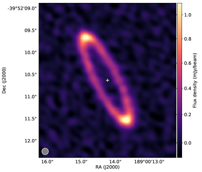
Figure 1: Self-calibrated Briggs-weighted image of the disk around HR 4796A (robust = 0.5). The filled circle in the lower left corner shows the beam of 0.16$\times$0.18″. The star is not detected but it’s location is marked by a +, and with a distance of 72.8pc the diameter of the ring is approximately 160au.

We first take a quick look at the observations using the clean image. Detailed visibility modelling is carried out below, so the purpose of this section is simply to introduce the data and provide a qualitative image-based feel for the results that will follow.

Figure 1 shows that the disk is seen very clearly as a narrow ring that is strongly detected (S/N$>$9) at all azimuths. The width of the disk appears similar to the beam size of 0.17″, so given the distance of 72.8 parsecs the radial and vertical extent of the ring about the maximum near 80au is no more than about 15au. The star is not detected, which is consistent with the predicted photospheric flux of 25.5$\mu$Jy.

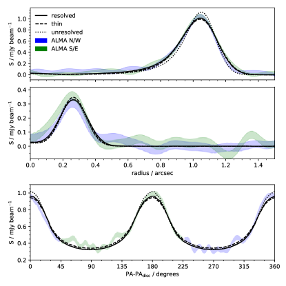
Figure 2: Radial (top two panels) and azimuthal (bottom panel) profiles of the surface brightness $S$. The radial profiles are along the disk major (upper panel) and minor (middle panel) axes, using 10^∘-wide swaths. The blue transparent bands show sections to the N and W, and the green to the S and E; the width of these bands is the 1$\sigma$ uncertainty. The same profiles are shown for three different models. The dotted lines show a model ring that is ‘unresolved’ radially and vertically. The dashed lines show a vertically ‘thin’ (flat) Gaussian model that is resolved radially, and the solid line shows a radially and vertically ‘resolved’ model. These models are described in detail in section 3.1. The unresolved model is a poor match to the data, and there is little difference between the resolved and thin models.

As a test of whether the ring is resolved, Figure 2 shows radial cuts along the major and minor disk axes, and an azimuthal profile around the disk. For comparison three different models that provide good fits to the data (and which are described below) are also shown. Comparing an ‘unresolved’ ring model (dotted line) with the data, the ring appears clearly resolved in the radial direction, but whether it is resolved vertically is less clear. Some clue may be given by the asymmetry in the inner and outer parts of the radial profile along the major axis; a vertically ‘thin’ model (dashed line) does not contribute as much flux as one that is ‘resolved’ both radially and vertically (solid line), but this difference is barely discernible. Comparison with the azimuthal profile yields similar results. Thus, while profiles along both the major and minor disk axes are affected by the radial and vertical structure, the differences here are small and models of the full dataset are needed to quantify them.

As a quick test of whether the ring is consistent with being symmetric, we rotated the image by 180^∘ and subtracted it from the un-rotated version. The star is not detected, so an x/y shift was allowed to optimise the subtraction. The result of this subtraction is an image that appears consistent with noise, suggesting that any brightness asymmetry that could arise from the disk eccentricity of 0.06 is not detected with ALMA. As the star is undetected, we cannot rule out the possibility that the disk is eccentric but has an azimuthally uniform surface density.

Using an elliptical mask with a semi-major axis of 1.75″ and semi-minor axis 0.4″ (the ratio derived for the dust ring below), we measure a total disk flux of $14.8\pm 1.5$ mJy, where the uncertainty is dominated by the 10% absolute calibration uncertainty. These values are consistent with $14.4\pm 1.9$mJy measured with SCUBA-2 (Holland et al., 2013) as part of the Survey of Nearby Stars (SONS) legacy programme (Holland et al., 2017). This agreement suggests that the ALMA observations have not resolved out significant flux on scales larger than seen in Figure 1.

2.2 Spectral data and CO

The fractional luminosity ($f=L_{\rm disk}/L_{\star}$) of the disk around HR 4796A is exceptional (0.5%), and the system is very young, so we considered that detection of either remnant primordial or secondary CO gas in this system was likely with ALMA. However, no clear signal is detected in the dirty continuum-subtracted data cube. To search more carefully for secondary CO under the assumption that it is co-located with the dust, we used the filtering method developed by Matrà et al. (2015) as implemented by Matrà et al. (2017b). In this framework only pixels where the disk is detected at $>$5$\sigma$ in the continuum are used, and spectra in each pixel of the imaged data cube are red or blue shifted to account for the expected radial velocity at that spatial location. This method assumes the best-fit dust disk geometry derived in section 3 and an estimated stellar mass of 2.18 M_⊙ (Gerbaldi et al., 1999). This method did not result in a detection and yields an integrated line flux upper limit (3$\sigma$) of 25 mJy km s^-1. A similar search for CO distributed in the same orbital plane as the disk, but with a different radial extent, also yielded a non-detection.

3 Continuum image Models

We now place more formal constraints on the disk parameters, modelling the disk as an optically thin torus using the observed visibilities. To reduce the computational load we temporally averaged the data into 10-second long chunks, and spectrally averaged the four spectral windows down to four channels per spectral window. Following averaging, the visibility weights were recomputed using the CASA statwt task. This step ensures that the relative visibility weights are correct, but not necessarily their absolute values, and this is corrected below.

The modelling method is the same as used by Marino et al. (2016, 2017). For one specific set of parameters a disk image is first generated using radmc-3d (Dullemond et al., 2012). This image is then Fourier transformed to the visibility plane, where the image is interpolated at the same $uv$ points as our time averaged continuum observations. The difference between the model and the data is then quantified by computing the $\chi^{2}$ goodness-of-fit metric over all visibility samples. In computing the $\chi^{2}$ we applied a constant re-weighting factor of 1/2.5 (i.e. we increase the variance by a factor of 2.5) that ensured the reduced $\chi^{2}$ for all visibilities was unity (i.e. the signal from the disk in an individual visibility sample is assumed to be negligible, which given $N_{\rm vis}=3210532$ separate visibilities to be modelled is reasonable, see also Guilloteau et al., 2011). This re-weighting ensures that the parameter uncertainties are realistic. Experiments where this factor was instead included as a model parameter find that it is very well constrained ($<$1% uncertainty), so we chose to use a constant value for all models.

To find the best fitting model for a given set of parameters, we use the ensemble Markov-Chain Monte-Carlo (MCMC) method proposed by Goodman & Weare (2010), as implemented by the emcee package (Foreman-Mackey et al., 2013). emcee uses an ensemble of ‘walkers’ (i.e. a series of parallel chains), which are used to inform the proposals at each step in the chain, increasing the efficiency of the sampler and allowing for parallel computation. For most fitting runs we use 40 walkers and chains with 1000 steps, increasing the number of steps in a few cases with strongly correlated parameters that take longer to fill out the parameter space. Each model is initialised near the optimal solution based on prior testing runs, so we typically only need to discard the first 100 steps as a ‘burn in’ phase.

We tried two families of models: symmetric and asymmetric. The goal of the symmetric models was to derive best-fit parameters and test whether the data show evidence for a specific disk radial profile and/or vertical distribution, and whether different choices for these influence other parameters. As was suggested in section 2.1 the disk appears symmetric, so the purpose of an asymmetric model was to verify that the disk is indeed consistent with being symmetric, and to quantify the level of asymmetry that could have been detected.

Parameters that are common to all models are the dust mass $M_{\rm dust}$, the average disk radius $r_{0}$, the disk position angle $\Omega$ (measured East of North), the disk inclination $I$, and the (small) sky offset of the disk from the expected location $x_{0}$, $y_{0}$. The disk is not significantly offset (0.025″) considering the $\sim$0.01″ pointing accuracy of ALMA and the S/N of our image, which limits the disk eccentricity to less than about 0.05 for a pericenter direction along the disk major axis (and less than about 0.2 for pericenter along the minor axis). Otherwise these latter two parameters are unimportant, so feature no further in our analysis. The data comprise two subsequent observations that are calibrated separately, so to allow for any differences we include a factor that is the fractional difference in calibration in the second observation relative to the first (i.e. we do not consider that the disk brightness actually changed over one hour at a location where the orbital period is about 500 years). These seven common parameters define the disk geometry, scale, and brightness, while the model specific parameters described below define the detailed radial and vertical structure.

For these models we assume a size distribution of dust from $D=10$$\mu$m to 1cm with a power-law slope $n(D)\propto D^{2-3q}$ with $q=11/6$. To compute the opacity needed by radmc-3d we use a mix of astronomical silicate, amorphous carbon, and water ice such that the 880$\mu$m opacity is 0.17 m² kg^-1 (45 au² $M_{\oplus}^{-1}$). As our observations are in a single narrow bandpass this choice is arbitrary and the mass is given largely for comparative purposes (i.e. it has a considerable systematic uncertainty).

Table 1: Best-fit parameters for the Gaussian, box, and power-law models. We follow previous authors’ conventions of $\sim$$26^{\circ}$ for the ascending node and $\sim$$77^{\circ}$ for inclination. Strictly, for this node the inclination should be $\sim$$103^{\circ}$ because the West side of the disk is closer to us (or the node should be $\sim$$206^{\circ}$ and the inclination retained). The dust mass uncertainty includes the contribution from the absolute flux calibration

	Gaussian		Box		Power-law
Parameter	Value	1$\sigma$	Value	1$\sigma$	Value	1$\sigma$
FWHMr (au)	10	1	-	-	5	1
FWHMh (au)	7	1	-	-	7	1
$\delta_{r}$ (au)	-	-	14	1	-	-
$\delta_{h}$ (au)	-	-	10	1	-	-
$M_{\rm dust}$ ($M_{\oplus}$)	0.35	0.04	0.35	0.04	0.35	0.04
$r_{0}$ (au)	78.6	0.2	78.4	0.2	78.4	0.2
$\Omega$ (∘)	26.7	0.1	26.7	0.1	26.7	0.1
$I$ (∘)	76.6	0.2	76.6	0.2	76.6	0.2

Table 2: Best-fit $\chi^{2}$ values relative to the Gaussian torus model (for which $\chi^{2}=3203624.3$). The number of model parameters, and the BIC values (relative to the Gaussian model) are also given.

Model	$\Delta\chi^{2}$	$N_{\rm param}$	$\Delta$BIC
Two power law torus	-5.3	10	9.6
Power law torus	-5.1	9	-5.1
Gaussian torus	0.0	9	0.0
Two Gaussian torus	0.3	10	15.3
Eccentric Gaussian torus	1.2	11	31.2
Box torus	6.6	9	6.6
Gaussian torus (‘thin’)	21.8	8	6.8
Gaussian torus (‘narrow’)	65.6	8	50.6
Gaussian torus (‘unresolved’)	114.2	7	84.2

3.1 Gaussian torus

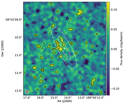
Figure 3: Naturally-weighted image of the residuals after subtracting the Gaussian torus model. Solid and dashed contours show the residuals at levels of -3, -2, 2, and 3$\sigma$. The star location is marked by a +, and white contours show the original image at 5$\sigma$. A pair of 3$\sigma$ contours remain within the disk near the semi-minor axis on the E side.

Our ‘reference’ model is a Gaussian torus of radius $r_{0}$, for which the additional parameters are the radial $\sigma_{r}$ and vertical $\sigma_{h}$ density dispersions. The full-width of the density at half-maxima FWHM_r and FWHM_h are therefore $2\sqrt{2\ln{2}}\approx 2.35$ times larger. The best-fit parameters for this model are given in Table 1, and the posterior distributions for all parameters in Figure 6 in the Appendix. A dirty image of the residuals, after subtracting the best-fit model in visibility space, is shown in Figure 3. The overall smoothness of the image shows that the model is a very good representation of the data. The $\chi^{2}$ value is 3203624; while this number is not informative in itself, comparison with the other models, summarised in Table 2, gives it some context. That is, the difference in $\chi^{2}$ values between different models is a more useful indicator of fit quality than the absolute values, so we quote these relative to this model below (e.g., Guilloteau et al., 2011).

Figure 3 shows one interesting feature; a pair of 3$\sigma$ residuals near the disk semi-minor axis on the East side. These appear for all models, with fluxes of around 100 $\mu$Jy. Inspection of residual plots for each observation shows that only one blob is present in each, suggesting that they are either spurious, or fluctuations caused by noise on top of a larger region of excess flux that is just below our sensitivity. Their location is near the disk apocenter inferred from scattered light observations (e.g. Milli et al., 2017), and whether they provide constraints on an apocenter glow scenario is considered below.

The basic conclusions from this model are that the disk can indeed be modelled as a narrow axisymmetric ring, and that the position angle and inclination are consistent with those derived from scattered light imaging (Rodigas et al., 2015; Milli et al., 2017, e.g. the latter find $I=76.45\pm 0.7^{\circ}$ and $\Omega=27.1\pm 0.7^{\circ}$). The radii derived from scattered light appear to differ systematically depending on the method, for example Rodigas et al. (2015) find values near 78au using a 10au-wide elliptical mask, while Milli et al. (2017) find values near 77au using a locus of the disk’s peak brightness. Our average disk radius is consistent with these results, though agrees more closely with Rodigas et al. (2015), presumably because their radius estimate is less biased by the $r^{-2}$ dependence for scattered light.

The radial and vertical extent of the disk is of particular interest here, and in addition to the search for CO provided the main motivation for obtaining high resolution images. The fitting results for the Gaussian model above find that the disk is resolved both radially and vertically, but given the modest signal to noise ratio seen in Figure 1, the lack of significant differences in Figure 2, and that the formal uncertainties on the radial/vertical extent are about a tenth of the resolution, we made some further tests.

First, we find that the disk is resolved in at least one of the radial or vertical directions, as an ‘unresolved’ model run where both $FWHM_{r}$ and $FWHM_{h}$ were fixed to $<$4au shows significant residuals, primarily near the ansae ($\Delta\chi^{2}=114.2$). In addition, a ‘narrow’ model where only $FWHM_{r}$ is $<$4au (and $FWHM_{h}$ is allowed to vary) also shows significant residuals ($\Delta\chi^{2}=65.6$). A ‘thin’ model where only $FWHM_{h}$ is $<$4au (and $FWHM_{r}$ is allowed to vary, yielding $FWHM_{r}=11$au) does not show any significant residuals aside from the same pair of blobs, but has $\Delta\chi^{2}=21.8$. While a smooth residual image might result because the disk is not vertically resolved, it could also arise because the preference for vertical extent is driven by a low-level signal spread across many beams (as is expected given that the disk itself spans many beams). The $\Delta\chi^{2}$ value for the thin model is higher than for all vertically resolved models (including the additional models described below), and is more similar to the value for the narrow case, so a vertically resolved disk is preferred.

A possibility that we have not yet explored is that a flat disk with a different radial profile parameterisation could account for the radial and apparent vertical disk extent. However, a model that has independently varying inner and outer Gaussian $\sigma_{r}$ (i.e. $\sigma_{\rm r,in}$ and $\sigma_{\rm r,out}$) still finds a non-zero $\sigma_{h}$ (and has $\Delta\chi^{2}=0.3$). We also tested the possibility that the residual blobs influence the results; adding a point source to the original Gaussian torus at the location seen in the first half of the visibility data finds that the disk is still vertically resolved.

3.2 Box torus

As a test of whether a torus with a different structure is also consistent with the ALMA data, we use a model with uniform space density within certain radial and vertical limits. A cross section through this torus yields a rectangular density distribution (i.e. a box), with radial width $\delta_{r}$ and vertical height $\delta_{h}$. While there is no more motivation for the radial structure than there was for the Gaussian model, a confined vertical structure could arise if the disk particles were being perturbed on secular (long) timescales by a slightly misaligned planet; the total height of the box would be twice the initial misalignment between the disk and the planet.

The results for the box model ($\Delta\chi^{2}=6.6$) are similar to the Gaussian torus (see Table 1), and again find that the disk is vertically resolved. Aside from the same peaks to the E of the star, the residuals are again consistent with noise. Bearing in mind that the horizontal and vertical extent reported for the box model is absolute, rather than representative in the Gaussian case, we consider the results of the two models essentially equivalent (though note that the $\Delta\chi^{2}$ is slightly higher for the box model). Thus, while we can measure the 3-dimensional structure of the disk in terms of the width and height for both models, we cannot easily discern among different possibilities for the details of how this dust is distributed within the torus.

3.3 Power-law torus

A final symmetric model retains the Gaussian vertical structure, but has a radial surface density profile described by a power-law. Specifically, the density is proportional to $\left[(r/r_{0})^{-2p_{\rm in}}+(r/r_{0})^{2p_{\rm out}}\right]^{-1/2}$. This profile is regularly used to model scattered light observations, and more specifically has been applied to the disk around HR 4796A (Augereau et al., 1999; Milli et al., 2017). By fitting power-laws to the radial profiles along the disk semi-major axis, the latter authors found $p_{\rm in}=23$, and $p_{\rm out}=13$ to $18$, so one aim with this model is to test whether the ALMA observations could be consistent with these parameters. Given the lower spatial resolution of our ALMA data relative to SPHERE, and the fact that the previous two models are both adequate descriptions of said ALMA data, we first set $p=p_{\rm in}=p_{\rm out}$. All other parameters are the same as in the Gaussian and box tori models.

The best fit power-law index for this model ($\Delta\chi^{2}=-5.1$) is $p=24\pm 2$, which corresponds to a FWHM of only 5au. The residuals are indistinguishable from the results of the previous two models, the $\Delta\chi^{2}$ value is slightly lower than the Gaussian torus model, and again the disk is found to be vertically extended with $FWHM_{h}=7$au. Relaxing the model to allow $p_{\rm in}$, and $p_{\rm out}$ to vary independently does not change this conclusion ($\Delta\chi^{2}=-5.3$). While these models are markedly narrower than the previous ones in terms of FWHM, this narrowness is not actually detectable with our ALMA resolution and the model width must be driven by the extended wings in the radial profile. We have nevertheless shown that the radial profile can be modelled with a power-law profile that is consistent with the higher spatial resolution scattered light data.

3.4 Eccentric Gaussian Torus

It is now well established from scattered light imaging that the disk around HR 4796A has an eccentricity of about 0.06, which at this level is well approximated as a circular disk whose center is offset from the star. While the exact magnitude of this offset shows small differences depending on the dataset and the method used to extract it, the results are largely consistent (see however section 4.5 for further discussion). These observations conclude that the apocenter of the disk is near the semi-minor axis of the disk on the East side, slightly below the location of the residual clumps seen in Figure 3. To test whether these clumps are indicative of an apocenter glow model, or constrain the eccentricity that could have been detected with ALMA, we use the simplified model of Pan et al. (2016) to prescribe the dust density around an elliptical annulus. Two additional parameters are required; the eccentricity of the belt $e$, and the argument of pericenter $\omega$ ($\omega$ is measured from the ascending node $\Omega$, so $\omega=0$ corresponds to a pericenter at the NE ansa). Despite the clumps this model finds that the eccentricity is consistent with zero, with an upper limit of 0.1 and no preference for any particular pericenter direction, and therefore shows no evidence for the offset ($\Delta\chi^{2}=1.2$). A probable reason that the apocenter glow model is not favoured is that the surface brightness should change smoothly around the ring, while the clumps are relatively localised.

Should we have detected apocenter glow? Pan et al. (2016) note that the ratio of the disk surface brightnesses at apocenter and pericenter tends to approximately $1+e$ at long wavelengths where flux density is linearly dependent on temperature. Thus, based on the eccentricity derived from scattered light, at most the ratio for HR 4796A’s disk should be about 1.06. The peak S/N in the clean image is 37 per beam (at the ansae), and by experimenting with regions of different sizes, a peak S/N of 73 was obtained for square regions 0.2″² centered on the ansae. A flux difference of $1/(73/\sqrt{2})=2$% between the ansae would be detected at 1$\sigma$, and the sensitivity for other opposing parts of the ring lower because the fraction of the ring within a given sky area is smaller. Thus, because the maximum ratio is not necessarily reached at 880$\mu$m, our non-detection of apocenter glow does not constrain the model.

3.5 Summary of modelling

In summary, we find that the dust ring around HR 4796A is strongly detected with ALMA, and that the parameters of our models are generally well constrained. All models find the same residual blobs near the semi-minor axis on the E side of the ring, but we do not consider them significant and note that their origin might be made clearer with lower resolution and/or deeper imaging. The ring is clearly radially resolved, and models where the disk is also vertically resolved yield the lowest $\chi^{2}$ values. This conclusion was robust to different models that might have accounted for an apparent vertical extent with a different radial profile. These tests were however not exhaustive.

Formally, we can use the Schwarz criterion (Bayesian Information Criterion, or BIC) to test which among our models should be preferred (Schwarz, 1978). This criterion tests whether the differences in $\chi^{2}$ values are large enough to be considered significant, including a penalty for models that have greater numbers of parameters: $BIC=\chi^{2}+N_{\rm param}\ln(N_{\rm vis})$. Differences in BIC values greater than six should be considered ‘strong’ evidence in favour of the model with the lower value (Kass & Raftery, 1995). The relative BIC values are given in Table 2, and show that the Gaussian and power-law torus models are preferred, with preference for the power-law model. The box torus and vertically unresolved (‘thin’) models are poor enough to have ‘strong’ evidence against them, which is despite the thin model having one less parameter. The BIC imposes a heavy penalty for additional model parameters because we have a very large number of visibilities, meaning that the addition of independently varying inner and outer power law and Gaussian profiles is not well justified given the small improvement in the fit. These formal tests largely confirm what we concluded above. While it remains possible that the disk is not vertically resolved, the evidence from our modelling suggests that it is.

Finally, it may be that the clumps are in fact astrophysical, and a sign that our models are too simple and do not account for underlying structure that is only marginally detected. In such a case our conclusions about the vertical extent could be incorrect because we have not considered all possible disk models. In section 4.5 we provide some evidence that alternative models merit consideration, and expect this issue to be resolved with higher resolution imaging.

4 Discussion

The primary conclusion from our ALMA data is that we have resolved the debris ring around HR 4796A radially, and probably vertically. In addition to the requirement of observing at high spatial resolution, this measurement is made possible by the intermediate inclination of the disk; we effectively measure the height near the semi-minor axis, and the width near the ansa, although they can only truly be backed out and the degeneracy quantified by self-consistent modelling (see Marino et al., 2016). Expressed as full-width half-maxima from the Gaussian torus model these radial and vertical extents are respectively 10 and 7au, and 14 and 10au for the box model. Compared to the disk mean radius of 79au, the radial width can be considered as an aspect ratio $w={\rm FWHM}_{r}/r_{0}=0.13$ (or $\delta_{r}/r_{0}=0.16$) and the vertical extent as a scale height $h={\rm FWHM}_{h}/(2r_{0})=0.04$ (or $\delta_{h}/(2r_{0})=0.07$). For the box model the height is equivalent to a maximum particle inclination of 3.5^∘ or opening angle of 7^∘, if particles’ ascending nodes are distributed randomly. Using a power-law radial profile model, we conclude that the width of the disk as seen with ALMA is consistent with the width seen in scattered light.

The vertical extent of the disk is important for the following discussion because this extent gives a direct measure of the range of orbital inclinations of the particles observed. Because the grains observed by ALMA are large enough to be weakly affected by radiation pressure, the structure is therefore also representative of larger bodies. With the assumption that their nodes are randomly oriented, these inclinations then set the minimum relative particle velocities and therefore the level of dynamical excitation in the disk. While the velocities may be higher if there are also relative radial velocities, these cannot be inferred from current observations because a ring of particles on concentric orbits with a range of semi-major axes looks the same as a ring of particles with a single semi-major axis and a range of eccentricities and pericenter directions.

This point provides a theoretical reason to be cautious about our conclusion regarding the vertical extent of the disk. As noted at the outset, Thébault & Wu (2008) propose that the narrow appearance of HR 4796A’s dust ring in scattered light arises because it is dynamically very cold (i.e. eccentricities and inclinations less than 0.01). In this case the dust size distribution is depleted in the smallest ($\sim$10$\mu$m) grains, because their velocities and destruction rate are increased relative to larger grains by radiation forces. These small grains typically have eccentric orbits and appear beyond the parent belt as a ‘halo’, so a disk that lacks them will appear unusually narrow in scattered light. Such a disk must be vertically thin, so would not appear to be vertically resolved by our observations.

While such a scenario may be attractive, and we consider its implications below, Thébault & Wu (2008) note that a serious issue is whether such low eccentricties and inclinations can actually be obtained. The debris disk paradigm requires a reservoir of parent planetesimals, which inevitably stir the disk to eccentricities and inclinations of order 0.01 unless they are smaller than a few kilometers in size.

4.1 Collisional status

Given that the stellar and disk properties are well known or can be estimated, the rate at which mass is being lost from the disk can be calculated with the assumptions that the emitting surface area of the disk is dominated by the smallest grains, and that these grains are always destroyed when they collide with each other (Eq. B6 in Matrà et al., 2017b). The latter assumption requires sufficient relative velocities between dust grains, which can be obtained in several ways. If the particle eccentricities are similar to the eccentricity of the ring and have a range of pericenter directions (i.e. their orbits are not concentric) the grain-grain collisions are probably destructive. The same applies if the disk has the vertical extent suggested by our modelling. In a very low-excitation scenario the assumptions become questionable because the smallest dust does not dominate the dust emission, and lower mass loss rates are possible.

The estimated mass loss rate is 26 $M_{\oplus}$ Myr^-1. This rate is very high compared to estimates for other stars (e.g. using the same calculation, 0.01 and 0.4 $M_{\oplus}$ Myr^-1 for Fomalhaut and HD 181327 respectively), primarily because HR 4796A’s disk has a very high fractional luminosity $f$ and the mass-loss rate is proportional to $f^{2}$. Given that the system age is approaching 10Myr, a prodigious mass in solids may therefore have been lost since dispersal of the gas disk, especially if the disk fractional luminosity was higher in the past. Given the caveat about the excitation level however, this rate could also be considered as an upper limit.

Comparison of this rate with estimates for the total mass in solids present is very uncertain, simply because this estimate requires an extrapolation up to the unknown maximum planetesimal size $D_{\rm c}$ (in km). Using equation (15) from Wyatt (2008), which assumes a size distribution with $n(D)\propto D^{2-3q}$ and $q=11/6$ (with $M_{\rm tot}$ in units of $M_{\oplus}$),

$$M_{\rm tot}=fr_{0}^{2}\sqrt{D_{\rm c}D_{\rm bl}}/0.37$$ (1)

and again assuming a $D_{\rm bl}=10$ (in $\mu$m) minimum size, yields $M_{\rm tot}=270\sqrt{D_{\rm c}}M_{\oplus}$ and therefore a mass of 270$M_{\oplus}$ for a size distribution up to 1km bodies. Rearranging equation (16) from Wyatt (2008), which connects the total mass, maximum planetesimal size, and collisional timescale, yields (with $t_{\rm coll}$ in Myr):

$$M_{\rm tot}=140D_{\rm c}/t_{\rm coll}$$ (2)

where we have also assumed planetesimal strength $Q_{\rm D}^{\star}=150$ J kg^-1 and eccentricity $e=0.05$ (this model makes various simplifying assumptions, e.g. that planetesimal strength is independent of size and that all material resides in a belt of fixed width). In this model $e$ simply sets the collision velocities, so is interchangeable with inclination, and decreasing either results in less frequent collisions and a longer collisional lifetime. Thus, if the dynamical excitation is lower, so is the inferred disk mass.

Equating (1) and (2) to eliminate $M_{\rm tot}$ and solve for $D_{\rm c}$ gives $D_{\rm c}=3.6t_{\rm coll}^{2}$, from which it can be concluded that bodies much larger than 1km must be present if the disk has been grinding down for $t_{\rm coll}$ equal to the system age, otherwise it would be fainter than observed. If the disk has been evolving for 10Myr up to 360km bodies are needed, corresponding to a disk mass of 5000$M_{\oplus}$. For a collisional evolution time of only 1Myr, 4km bodies could be colliding, and the total disk mass 500$M_{\oplus}$. If we assume $e=0.01$, 2km bodies are needed and the disk mass is 350$M_{\oplus}$.

To put these estimates in perspective, a 26$M_{\oplus}$ ‘isolation mass’ object (Lissauer, 1987) would form from material within a similar radial extent as the ring around HR 4796A, and corresponds to a surface density of 0.1 g cm^-2 ($2.7M_{\oplus}$ au^-2), similar to the solid component of the ‘minimum mass Solar nebula’ at this distance (Weidenschilling, 1977). Similar surface densities have also been estimated for protoplanetary disks (e.g. Andrews et al., 2009).

These very high disk masses may present a problem; if the disk is not dynamically cold the collision rates are such that requiring a reasonable disk mass ($<$100$M_{\oplus}$, say, remembering that all of this mass is confined to the observed ring) requires that the largest planetesimals be smaller than kilometers in size, but the lifetime of the disk at the observed level is then much shorter than the system age ($<$1Myr). Conversely, requiring that the disk be able to survive at the observed level for a sizeable fraction of the system age requires large ($>$100km) planetesimals, and therefore a very large disk mass. This mass problem is not unique to HR 4796A, and possible solutions arise when assumptions made above are relaxed, such as the strength of the planetesimals and their size distribution, that dust only originates in collisions, or that the systems have been colliding for shorter than the apparent stellar age. See Krivov et al. (2017) for a general discussion of this issue.

As noted above, both the disk mass and mass loss rate problems are related to the vertical extent of the disk, and both are also alleviated if the disk is dynamically very cold. In addition, the smaller planetesimals required would stir the disk less, meaning that the low excitation could be consistent with the expected level of stirring from the planetesimals (though whether a lack of $\gtrsim$1km planetesimals is consistent with planet formation models is debatable, see Krivov et al., 2017). The mass and mass loss rate issues might therefore be resolved if higher resolution observations showed that the disk is in fact thinner than our modelling suggests.

4.2 CO gas

4.2.1 CO mass upper limit

In section 2.2, we derived an upper limit to the observed integrated line flux of the ¹²CO J=3-2 transition for gas co-located with the debris ring. We now translate this flux into an upper limit on the total CO mass in the belt and aim to understand the origin of any CO that may still be present below our sensitivity limit.

To quantify the implications of this limit, we calculate the population of the upper level of the transition (J=3) with respect to all other energy levels of the CO molecule, using an improved version of the non-local thermodynamic equilibrium (NLTE) analysis of Matrà et al. (2015) that now includes the effect of fluorescence excitation (Matrà et al. submitted).

To calculate collisional excitation, we assume the main collider species to be electrons, as they have been shown to be the most likely to dominate collisions with CO in second-generation gas (e.g. Kral et al., 2016; Matrà et al., 2017a); collision rates are obtained from Dickinson & Richards (1975). Regardless, the CO mass derived from our flux upper limit is independent of our choice of collisional partner (e.g. Matrà et al., 2015).

To calculate radiative excitation, we consider the radiation field impinging on a CO molecule at the debris ring’s center, including stellar emission at UV to IR wavelengths (affecting electronic and vibrational transitions), as well as dust continuum and CMB emission at far-IR to mm wavelengths (affecting rotational transitions). The stellar emission is taken as that of a 9650K PHOENIX model atmosphere (Brott & Hauschildt, 2005, the temperature derived by fitting to optical photometry), whereas the dust continuum radiation field is measured assuming our best-fit dust model at 0.88 mm and scaling it to other far-IR/mm wavelengths using the observed SED. The PHOENIX models are of the stellar photosphere, so the UV emission could be higher. However, HR 4796A was detected between 1500 and 3000nm by the UV Sky-Survey Telescope in the TD-1A satellite (Boksenberg et al., 1973).. Aside from one value that is about 20 percent higher, the fluxes are consistent with our photosphere model, so there is no evidence of a significant UV excess.

We then proceed to solve the system of equations of statistical equilibrium to obtain the fractional population of our level of interest ($x_{\rm J=3}$) as a function of the unknown electron density (which we varied between 10^-3 and 10¹² cm^-3) and kinetic temperature (which we varied between 10 and 250 K). Finally, we assume that CO emission is optically thin and use Eq. 2 from Matrà et al. (2015) to derive a CO mass upper limit from our observed integrated flux upper limit, again as a function of electron density and kinetic temperature. We find a CO mass upper limit ranging between (1.2 to 3.7) $\times$ 10^-6 M_⊕, where this range is effectively independent of the electron density assumption, and only weakly dependent on our already wide range of temperatures assumed; we therefore adopt 3.7 $\times$ 10^-6 M_⊕ as the strict upper limit on the CO mass derived from our data.

4.2.2 Primordial origin of undetected CO excluded

To assess whether any undetected CO could be left over from the protoplanetary phase of evolution, we need to consider whether i) such a low CO mass could be optically thick to the line of sight, causing our CO mass upper limit to be underestimated and ii) whether CO could have survived photodissociation from the central star since the end of the protoplanetary phase of evolution. In order to do so we draw an analogy with the Fomalhaut ring, since it has a similar radial extent and inclination to that of HR 4796A (MacGregor et al., 2017), leading to a similar column length that a CO molecule in the center of the ring ‘sees’ towards the star ($\sim$6.5 AU), and a similar column length of CO throughout the ring along the line of sight to Earth ($\sim$13 AU). Assuming a uniform density torus, the maximum CO number density in the HR 4796A ring is 2.1 cm^-3, leading to maximum column densities of 2.0 and 4.0$\times$10¹⁴ cm^-2, respectively.

Using Eq. 3 from Matrà et al. (2017a), for the whole range of electron densities and kinetic temperature considered above, we set an upper limit to the optical thickness of the ¹²CO J=3-2 line along the line of sight to Earth of $\tau_{\rm 345GHz}\leq 0.4$. This shows that our optically thin assumption is a good approximation and most likely valid for any CO co-located with the debris ring. Furthermore, the results of Visser et al. (2009) indicate that the maximum column density of CO along the line of sight to the star leads to very little self-shielding against photodissociating UV photons; even when including the shielding effect of a potential primordial H₂ reservoir with a low CO/H₂ ratio of 10^-6, the increase in CO lifetime against photodissociation is only a factor $\sim$5.

Using the same model stellar spectrum as above, and the modified Draine (1978) interstellar UV field of van Dishoeck et al. (2008), together with photodissociation cross-sections from Visser et al. (2009), we derive a photodissociation timescale of eight years at the radial location of the ring’s centre. HR 4796A is an A0-type star, and as such has a relatively high UV luminosity, so the lifetime of CO is much shorter than the 120 years typically assumed when CO dissociation is driven solely by interstellar ultraviolet photons (Visser et al., 2009; Matrà et al., 2015; Kral et al., 2017). We therefore conclude that any CO present in the HR 4796A ring below our detection threshold cannot have survived for more than $\sim$40 years, ruling out the hypothesis that primordial CO gas could have survived since the protoplanetary phase of evolution.

While these estimates are based on CO that is restricted to be co-located with the dust (expected because the CO lifetime is much shorter than the orbital period at that distance), we estimate that the lifetime of a broader distribution would still be very short. If we assume a CO disk with the same number density as our upper limit that extends all the way to the star, the radial column density would be a factor $\approx$10 higher. For the same CO/H₂ ratio assumed above the photodissociation time therefore increases by a factor of a few, but is still significantly shorter than the age of the system.

4.2.3 The CO+CO₂ ice reservoir in HR 4796A’s exocomets

Given the short lifetime of any CO that is co-located with the debris ring, any such gas that exists below our detection limit must originate in the planetesimals that feed the observed dust. Other studies have used the steady-state mass-loss rate from the collisional cascade, in concert with a CO detection or upper limit and a CO lifetime, to estimate or set limits on the fraction of CO and CO₂ ice in the parent planetesimals.

Taking our measured CO mass upper limit, the derived CO lifetime of eight years indicates a CO mass loss rate of $<0.46$ M_⊕ Myr^-1. In steady state, this rate can be combined with the estimated mass loss rate from the collisional cascade (section 4.1) to measure an upper limit of $<$1.8% on the CO+CO₂ ice mass fraction in exocomets within the HR 4796A ring. This fraction is lower than the CO+CO₂ mass fractions estimated for Solar System comets and the Fomalhaut system (see Matrà et al., 2017b), but comparable with the estimate for the debris ring around the F2 type star HD 181327 (Marino et al., 2016). As noted above, this fraction is uncertain because it relies on the uncertain dust mass loss rate, and could therefore be higher if the disk is vertically thin (in which case this mass loss rate is considered an upper limit, and could be much lower). As before, quantifying the vertical extent of the disk can resolve this issue.

4.3 Radial width and comparison with scattered light

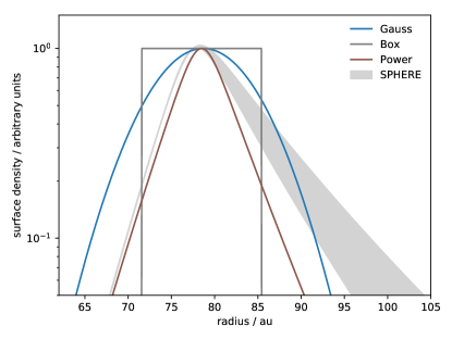
Figure 4: Radial profiles of the main models from section 3 (solid lines) and the 1/$r^{2}$-corrected scattered light flux profile from SPHERE observations (grey line and filled region). The spatial resolution of our ALMA observations is about the same as the width of the box model (FWHM = 12.4au). The vertical range of the plot is chosen to approximately reflect the signal to noise ratio of the observations.

One of the primary drivers for obtaining these data was to compare the radial distributions of larger grains, as seen with ALMA, with the smallest grains, as seen in scattered light. For this comparison, we use the results of Milli et al. (2017), who measure a FWHM_r of 7au using a power-law model (by measuring the width along the semi-major axis). As shown in section 3.3 the best fitting power-law model is consistent with that derived from the scattered light data. However, as highlighted by the range of radial widths derived from the models, our resolution is insufficient to say whether the dust as seen by ALMA is as radially concentrated as it appears in scattered light. The diversity of possibilities is illustrated in Figure 4, which shows the radial profiles of the Gaussian, box, and power-law models. For comparison, the power-law fit to the SPHERE data along the disk’s major axis is also shown, where the range covered by the gray filled region shows the difference between the outer profiles seen towards the NE and SW ansae (Milli et al., 2017).

We conclude that the radial extent of the smallest grains in the disk as imaged by SPHERE appears to be very similar to that for larger $\sim$mm-sized grains as imaged by ALMA. This similarity is unexpected, because dust near the blowout limit should reside on high-eccentricity orbits, creating a ‘halo’ beyond their source region that has a scattered light surface brightness power-law profile of $r^{-3.5}$ (Strubbe & Chiang, 2006; Krivov et al., 2006; Thébault & Wu, 2008). As noted above, one explanation could be the low planetesimal excitation scenario, while a related possibility is that the ring is radially optically thick. Another scenario is shepherding by an outer planet (Lagrange et al., 2012).

The outer shepherding planets considered by Lagrange et al. (2012) had masses in the range 3 to 8$M_{\rm Jupiter}$, which, aside from uncertainties in the conversion between mass and brightness, are not favoured by more recent direct imaging Milli et al. (2017), so we consider this possibility unlikely.

Considering the high radial optical depth scenario (which prevents small dust from leaving the ring before it is destroyed), Thébault & Wu (2008) find that radial optical depths of order unity are required for the halo to be significantly attenuated. If the disk is vertically resolved then the radial optical depth is $fr_{0}/h\approx 0.1$, and it seems implausible that the radial optical depth in the HR 4796A disk is sufficiently high to be responsible for the lack of a small-grain halo. Similarly, if our measurement of the vertical scale height for the disk is correct, low planetesimal excitation is implausible and would rule out this possibility. Thus, in addition to having implications for the uncertain disk mass and mass loss rate, further mm-wave observations can help understand the role of radial optical depth and dynamical excitation in setting the steep radial profile seen in scattered light.

4.4 Expectations from secular perturbations

What do the various measurements mean, if anything, for the history and status of the debris ring? If we assume that the offset seen in scattered light and the pericenter glow seen in the mid-infrared arise from a planet-induced (‘forced’) eccentricity $e_{\rm f}$ within the disk of about 0.06 (but see section 4.5 for discussion of this assumption), then the present appearance of the ring depends on the initial conditions, which we now discuss. We then consider how secular perturbations set constraints on the putative planet’s mass and semi-major axis. If the disk is vertically resolved further constraints are possible, because the lifetime of the disk as it currently appears is inferred to be short.

4.4.1 Initial conditions

Considering the vertical extent first, any initial misalignment between the planet and the disk causes the bodies’ ascending nodes to precess. The precession rate is a function of semi-major axis, so for a disk of finite width differential precession eventually randomises the nodes of neighbouring planetesimals, and the final vertical extent of the disk is twice the initial misalignment. Thus, our inferred vertical extent could arise from a very flat disk initially inclined 3.5^∘ relative to the planet. However, the vertical extent could equally arise because this was the intrinsic range of inclinations, but this scenario requires that any initial planet-disk misalignment was very small. The way to distinguish between these possibilities is to measure the vertical density distribution; in the former scenario the density will be highest at the highest inclinations (Neugebauer et al., 1984, see also section 3.2), while for the latter the density is almost certainly more concentrated towards the mid-plane. If the disk is vertically very thin, and a planet causes the disk eccentricity, then any initial misalignment was very small.

The argument for the radial extent is similar, but any scenario must also satisfy the observed eccentricity. Secular perturbations from a planet with semi-major axis $a_{\rm pl}$ impose a forced eccentricity and longitude of pericenter $\varpi_{f}$; the orbit of any body that already has these values for $e$ and $\varpi$ will not change, while the $e$ and $\varpi$ of any other body will change such that the highest eccentricity occurs when the pericenter is aligned with the planet’s (along $\varpi_{f}$). Thus, the width of a disk can either reflect the disk’s initial width, as long as the initial eccentricity happened to be at the forced location, or the disk could have initially been narrow with low eccentricity and the width mostly contributed by pericenter precession. By ‘mostly’, we mean that the width cannot be solely contributed by pericenter precession because if all planetesimals were all initially at the same semi-major axis $a$, then there would be no differential precession and the disk would only ever be a narrow ring whose pericenter precesses. A finite width means that differential precession due to different semi-major axes can eventually randomise the orbits (‘phase mix’ in $e\cos\varpi$, $e\sin\varpi$ space) and pericenter glow set up (Wyatt, 2005). If we simply assume that the initial width is narrower than the observed width ($\lesssim$5au), then the width expected from precession is about $2ae_{f}$, which is similar to that measured.

Which of these origins is more likely? The fact that the disk width is close to that expected given an initial distribution that was both narrow and on circular orbits may favour this initial condition. However, it also seems possible that the orbits of a population of planetesimals orbiting exterior to a planet could ‘relax’ to the forced values due to some dissipative process, the prime candidate being gas drag before and during gas disk dispersal. In either case, the presence of an exterior planetesimal population might be the result of a ‘pile up’ of dust in the gas pressure maximum just external to a planet (Pinilla et al., 2012), and the most likely initial conditions predicted by further development of such models. Occam’s razor suggests that the planet that caused the pile-up, and the planet causing the observed disk to be offset from the star, are one and the same.

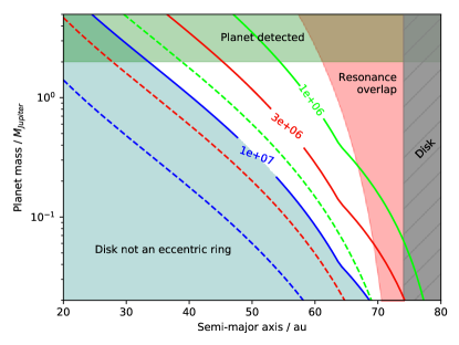
Figure 5: Limits on locations of an interior planet that imposes the eccentricity of the HR 4796A debris ring. The solid contours show the mass and semi-major axis of planets that cause the disk to appear eccentric after the times given by each label. The dashed lines show the mass and semi-major axes for the onset of collisions at the same times. Planets above about 2 $M_{\rm Jupiter}$ would have been detected, planets too close to the disk would eject particles via resonance overlap, and planets too far away would not force the ring to be eccentric within the lifetime of the star. The equations used to generate this plot are given in Appendix B

4.4.2 Planet constraints

What kind of planet could impose the structure on the disk? Continuing with the picture of an interior planet, the primary requirements are i) that the planet’s semi-major axis and eccentricity result in a forced eccentricity $e_{\rm f}=0.06$ at 79au (see Appendix B), and ii) that the planetesimals have undergone sufficient precession at 79au within some time (e.g. the age of the system, or the time elapsed since gas-disk dispersal). Based on a rough maximum initial width of 5au (see above), we quantify ‘sufficient’ by requiring that planetesimals 2.5au exterior to 79au have precessed through at least one full cycle, and that planetesimals 2.5 interior to 79au are at least one precession cycle ahead of those at the outer edge. Given the discussion above about the relation between initial and final disk widths, this condition is an approximation, but does not significantly affect our conclusions. This differential precession condition is very similar to the orbit-crossing criterion of Mustill & Wyatt (2009), the main difference being that particles need not precess a full cycle farther than their neighbours for their orbits to cross.

In general, the closer the planet to the disk, the more rapidly the disk is affected, so which condition dominates the phase-mixing requirement depends on the planet location; differential precession is slower than outer-edge precession when the planet is more distant from the disk. However, a planet cannot lie arbitrarily close to the disk, as it would remove bodies on short timescales, and therefore must lie farther than required by the resonance-overlap criterion (Wisdom, 1980).

The resonance-overlap and precession criteria, plus an approximate planet detection limit of 2 Jupiter-masses (Milli et al., 2017), are shown in Figure 5 (the equations used to generate this plot are given in Appendix B). Shaded regions at the upper and right boundaries of the figure show the regions of parameter space that are ruled out by resonance-overlap and planet detection limits. The solid lines show contours along which sufficient precession has occurred within 1, 3, and 10Myr. For times greater than 10 Myr, the disk has not precessed enough to appear as a uniform eccentric ring, which provides the third diagonal criterion to the lower left that bounds the planet location.

Where might an interior planet reside? The longer the disk has been in a state where secular perturbations can act as assumed (i.e. since gas disk dispersal) the lower the mass and the farther from the disk this planet can be. Given the estimated system age near 10Myr, the appropriate contour in Figure 5 in this scenario probably lies between 3 and 10Myr, meaning that roughly speaking the putative planet should be more massive than Neptune, and within 40au of the disk.

So far the constraints on this supposed planet have been purely set by dynamics, considering the time taken for the debris ring to appear as it does given plausible initial conditions. If the disk is vertically thin, it could be dynamically cold and collisions may be relatively unimportant (i.e. there are no mass loss rate or disk mass problems), and no more constraints are possible. However, if the disk has the vertical extent suggested by our modelling then the disk lifetime at the current brightness should be very short, and the inferred disk mass very large. This problem can be alleviated if the onset of collisions was relatively recent, which is possible if these collisions were initiated by the same perturbations that cause the disk to appear eccentric.

To this end, Figure 5 also shows contours of constant collision-onset times (using the method outlined by Mustill & Wyatt, 2009, but without the assumption of $a_{\rm pl}/r_{0}\ll 1$). These assume that collisions begin when disk particles have precessed sufficiently that their orbits overlap. For a given planet collisions begin well before the disk has precessed to the point that it appears smooth and eccentric, so the dashed contours are well below the solid ones. The onset of collisions is sufficiently short that the disk would have been losing mass for essentially the entire time taken for secular perturbations to make the disk appear eccentric. Thus, to avoid the disk mass problem the disk should have acquired the eccentric structure recently, so that the time since the onset of collisions is also short. This requirement does not necessarily mean that the gas-rich phase of disk evolution only ended recently, as the planet may have obtained an orbit necessary to stir and perturb the disk some time well after gas dispersal (e.g. by interaction with a second planet). Regardless, the preferred current planetary parameters are in the upper right of the allowed space; within 10-20au of the disk inner edge and with a mass similar to Jupiter.

This disk lifetime problem may also be alleviated by allowing the orbit of the planet to acquire the eccentricity necessary to stir and perturb the disk some time well after gas dispersal, for which a probable mechanism would be interaction with a second planet. Such a scenario is less attractive because of the added complexity, but is hard to rule out.

4.5 Alternative scenarios

While the eccentric nature of the ring has led to secular perturbation induced pericenter-glow being the favoured interpretation for the ring around HR 4796A, there remain issues with this interpretation that we now outline. The need for reconciliation of these issues points to alternative hypotheses.

The pericenter-glow hypothesis is based on mid-IR observations (Wyatt et al., 1999; Telesco et al., 2000; Moerchen et al., 2011), which have relatively low spatial resolution. The relevant observable is therefore the flux ratio between the two ansae. The constraints on the disk’s forced eccentricity and pericenter are degenerate, with the derived eccentricity being minimal (about 0.06) when the pericenter is at the NE ansa (Moerchen et al., 2011). The eccentricity can be higher, but to ensure the brightness asymmetry does not become too great the pericenter must be moved away from the ansa. This degeneracy is not total however, and Moerchen et al. (2011) show that it can be broken by considering the temperature profile along the disk semi-major axis. Using this constraint they conclude that the pericenter is near the NE ansa, though quote an uncertainty of 30^∘. However, for pericenters that are far from the ansa the eccentricity becomes much larger than 0.06, for example 0.3 when $\omega=\pm 75^{\circ}$.

The disk offset can be measured directly through high resolution imaging. In this case an ellipse with a non-zero stellocentric offset is fitted to the disk image, and the resulting parameters de-projected to yield the orbital elements of the ring. Several measurements have been made for this offset using scattered light imaging, which consistently find a small but non-zero eccentricity ($<$0.1, Schneider et al., 2009; Thalmann et al., 2011; Wahhaj et al., 2014; Rodigas et al., 2015; Milli et al., 2017). The arguments of pericenter vary somewhat, but are consistently closer to the semi-minor axes than they are to the ansa (suggesting that the scattering phase function is not influencing the results), and not consistent with a pericenter near the NW ansa. These results are therefore in conflict with those derived from pericenter glow in the mid-IR.

While these details do not point to specific alternative scenarios, they force us to consider relaxing modelling aspects that are commonly implicit in most debris disk models. One possible resolution is that the point in the disk that is closest to the star is indeed near the semi-minor axis on the Western side of the star, but the dust actually tends to be brighter near the NW ansa. To ensure that the $\sim$10K colour difference between the NE and SW ansae seen in the mid-IR is also satisfied, merely increasing the amount of dust would not be sufficient. The simplest explanation is that the dust at the NE ansa tends to be smaller, and therefore hotter and brighter than elsewhere in the disk. Such a difference in grain sizes might also be associated with an increase in space density, as an increased collision rate at a more dense disk location could cause an increase in the amount of small dust near that location.

Thus, an alternative picture for the disk around HR 4796A essentially involves decoupling the disk brightness and the geometry. The enhanced brightness and dust temperature at the NE ansa results from dust that is smaller on average. Secular perturbations may still be invoked for the ring eccentricity, but other ideas are possible. For example, the bulk of the dust in the ring may be the result of a single previous collision, which has since spread into a largely, but not entirely, uniform ring (Jackson et al., 2014). In this scenario, the ring retains the orbit of the progenitor, providing the origin of the ring’s eccentricity, and collisions are more frequent at the original collision location, which explains the increased dust temperature near the NE ansa.

The development of such alternative models is not the goal of this paper, but comparison of the mid-IR and scattered light results, and considering the implications of the collisional status of the system, suggests that there is sufficient evidence that their exploration is well motivated. The residuals seen in Figure 3, near the apocenter as derived from scattered light (the semi-minor axis on the Eastern side), may provide further motivation, though further observations to test whether they are real are desirable.

5 Summary and Conclusions

We have presented the first high spatial resolution mm-wave images of the debris disk around the young star HR 4796A, revealing a narrow ring of roughly mm-sized grains. Modelling of the radial and vertical structure with a variety of axisymmetric models shows that we have resolved the disk radially, with a $\sim$10au extent that is consistent with that seen in scattered light. These models consistently find that the disk is also vertically resolved, with a similar extent. Residual images show that these models provide a very good fit to the data; the only remaining structure is a few 3$\sigma$ blobs near the semi-minor axis on the East side of the star. We remain cautious about the claim of vertically resolved structure because it is smaller than the beam size, but find that it is robust to models that use a range of different radial profiles.

Various solutions have been proposed for the narrowness of the disk in scattered light. One that seems promising is a low excitation scenario that preferentially depletes the smallest dust (Thébault & Wu, 2008). This scenario is attractive because it provides a way to lower estimates of high disk mass and mass loss rates. However, this scenario is in conflict with our conclusion that the disk is vertically resolved, so higher resolution observations that confirm or refute the vertical extent would be very valuable for considering the dynamical excitation and collisional status of the belt.

We do not detect any CO gas, and rule out the possibility that any remaining undetected CO gas is primordial. Under the assumption that the disk is vertically resolved, we set an approximate limit on the CO+CO₂ ice fraction in the parent planetesimals of $<$1.8%. This value is at the low end of abundances observed in Solar System comets and other similarly aged exocometary belts, but could be higher if the disk has low dynamical excitation because the the mass loss rate used in the estimate would be lower.

We consider a scenario where the disk eccentricity arises from secular perturbations from an interior planet. Such a planet may be the reason the ring exists, having trapped radially drifting dust just exterior to its orbit during the gas-rich phase of evolution. Using constraints that bound its location and mass, we find that such a planet should be more massive than Neptune, and lie exterior to 40au.

Finally, we highlight a conflict between the interpretations of mid-IR and scattered light observations. While both suggest ring eccentricities of about 0.06, the former argues for a pericenter near the NE ansa, while the latter consistently finds the pericenter near the semi-minor axis on the West side of the star. These conclusions do not appear reconcilable, so we suggest that models that allow the spatial dust density and grain size to vary as a function of azimuth, independently of the pericenter location, should be considered.

Appendix A Modelling results

Figure 6 shows posterior distributions for all parameters from the ‘reference’ Gaussian torus model of section 3.1. The distributions show that the parameters are well constrained and show little degeneracy.

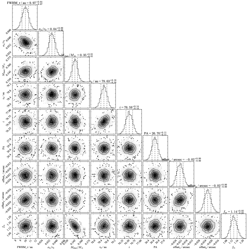
Figure 6: An example showing the posterior distributions of parameters from the MCMC fitting, in this case for the Gaussian torus model. In off-diagonal panels the solid lines show 1, 2, and 3$\sigma$ contours and the greyscale shows the density, and in the diagonal panels the histograms show the 1D distribution for each parameter, titled by the median and $\pm$1$\sigma$ uncertainty.

Appendix B Planet constraints

This section details the constraints used to generate Figure 5. Values assumed are $r_{0}=79$au, $e_{f}=0.06$, and $M_{\star}=2.18M_{\odot}$

B.1 Resonance overlap

The region marked ‘Resonance overlap’ is set by the resonance overlap criterion of (Wisdom, 1980), at which point:

$$a_{\rm pl}=r_{\rm in}\left[1-1.3\left(\frac{M_{\rm pl}}{M_{\star}}\right)^{2/7}\right]$$ (3)

where the inner disk edge $r_{\rm in}$ is assumed to be $r_{0}$ minus half the observed Gaussian disk width of 10au.

B.2 Secular perturbations

The eccentricity $e_{\rm pl}$ of a planet with semi-major axis $a_{\rm pl}$ that results in planetesimals at $r_{0}$ with eccentricities $e_{f}$ is given by

$$e_{\rm pl}=e_{f}b_{3/2}^{(1)}(\alpha)/b_{3/2}^{(2)}(\alpha)$$ (4)

where $b_{s}^{(j)}$ are Laplace coefficients and $\alpha=a_{\rm pl}/r_{0}$.

These Laplace coefficients can be written as:

$$b_{3/2}^{(1)}=3\alpha\mathcal{F}(3/2,5/2,2,\alpha^{2})$$ (5)

$$b_{3/2}^{(2)}=15\alpha^{2}\mathcal{F}(3/2,7/2,3,\alpha^{2})/4$$ (6)

where $\mathcal{F}$ is the standard hypergeometric function.

The secular precession frequency of planetesimals at $r$ under the influence of this planet is

$$A(r)=\frac{n}{4}\frac{M_{\rm pl}}{M_{\star}}\frac{a_{\rm pl}}{r}b_{3/2}^{(1)}(\alpha)$$ (7)

where $n=\sqrt{GM_{\star}/r^{3}}$ is the mean motion at $r$.

The precession time at the outer edge is then $2\pi/A(r_{\rm out})$, and the differential precession time between the inner and outer disk edges $2\pi/[A(r_{\rm in})-A(r_{\rm out})]$. Because the precession widens the disk, we use $r_{\rm in}=r_{0}-2.5$au and $r_{\rm out}=r_{0}+2.5$au here (i.e. an approximate initial width, which is narrower than the observed width). The lines in Figure 5 show the greater of these two quantities.

The crossing timescale given by Mustill & Wyatt (2009) is used, but without the simplifying assumption that $a_{\rm pl}\ll r$:

$$t_{\rm cross}=-1/(e_{f}\,r\,dA/dr)$$ (8)

where we use a numerical derivative for $dA/dr$.

References

- Acke et al. (2012) Acke, B., Min, M., Dominik, C., Vandenbussche, B., Sibthorpe, B., Waelkens, C., Olofsson, G., Degroote, P., Smolders, K., Pantin, E., Barlow, M. J., Blommaert, J. A. D. L., Brandeker, A., De Meester, W., Dent, W. R. F., Exter, K., Di Francesco, J., Fridlund, M., Gear, W. K., Glauser, A. M., Greaves, J. S., Harvey, P. M., Henning, T., Hogerheijde, M. R., Holland, W. S., Huygen, R., Ivison, R. J., Jean, C., Liseau, R., Naylor, D. A., Pilbratt, G. L., Polehampton, E. T., Regibo, S., Royer, P., Sicilia-Aguilar, A., & Swinyard, B. M. 2012, A&A, 540, A125
- Andrews et al. (2009) Andrews, S. M., Wilner, D. J., Hughes, A. M., Qi, C., & Dullemond, C. P. 2009, ApJ, 700, 1502
- Astropy Collaboration et al. (2013) Astropy Collaboration, Robitaille, T. P., Tollerud, E. J., Greenfield, P., Droettboom, M., Bray, E., Aldcroft, T., Davis, M., Ginsburg, A., Price-Whelan, A. M., Kerzendorf, W. E., Conley, A., Crighton, N., Barbary, K., Muna, D., Ferguson, H., Grollier, F., Parikh, M. M., Nair, P. H., Unther, H. M., Deil, C., Woillez, J., Conseil, S., Kramer, R., Turner, J. E. H., Singer, L., Fox, R., Weaver, B. A., Zabalza, V., Edwards, Z. I., Azalee Bostroem, K., Burke, D. J., Casey, A. R., Crawford, S. M., Dencheva, N., Ely, J., Jenness, T., Labrie, K., Lim, P. L., Pierfederici, F., Pontzen, A., Ptak, A., Refsdal, B., Servillat, M., & Streicher, O. 2013, A&A, 558, A33
- Augereau et al. (1999) Augereau, J. C., Lagrange, A. M., Mouillet, D., Papaloizou, J. C. B., & Grorod, P. A. 1999, A&A, 348, 557
- Backman & Paresce (1993) Backman, D. E. & Paresce, F. 1993, in Protostars and Planets III, ed. E. H. Levy & J. I. Lunine, 1253–1304
- Bell et al. (2015) Bell, C. P. M., Mamajek, E. E., & Naylor, T. 2015, MNRAS, 454, 593
- Boksenberg et al. (1973) Boksenberg, A., Evans, R. G., Fowler, R. G., Gardner, I. S. K., Houziaux, L., Humphries, C. M., Jamar, C., Macau, D., Malaise, D., Monfils, A., Nandy, K., Thompson, G. I., Wilson, R., & Wroe, H. 1973, MNRAS, 163, 291
- Brott & Hauschildt (2005) Brott, I. & Hauschildt, P. H. 2005, in ESA Special Publication, Vol. 576, The Three-Dimensional Universe with Gaia, ed. C. Turon, K. S. O’Flaherty, & M. A. C. Perryman, 565
- Burrows et al. (1997) Burrows, A., Marley, M., Hubbard, W. B., Lunine, J. I., Guillot, T., Saumon, D., Freedman, R., Sudarsky, D., & Sharp, C. 1997, ApJ, 491, 856
- Burrows et al. (1995) Burrows, C. J., Krist, J. E., Stapelfeldt, K. R., & WFPC2 Investigation Definition Team. 1995, in Bulletin of the American Astronomical Society, Vol. 27, American Astronomical Society Meeting Abstracts, 1329
- Chavez-Dagostino et al. (2016) Chavez-Dagostino, M., Bertone, E., Cruz-Saenz de Miera, F., Marshall, J. P., Wilson, G. W., Sánchez-Argüelles, D., Hughes, D. H., Kennedy, G., Vega, O., De la Luz, V., Dent, W. R. F., Eiroa, C., Gómez-Ruiz, A. I., Greaves, J. S., Lizano, S., López-Valdivia, R., Mamajek, E., Montaña, A., Olmedo, M., Rodríguez-Montoya, I., Schloerb, F. P., Yun, M. S., Zavala, J. A., & Zeballos, M. 2016, MNRAS, 462, 2285
- de la Reza et al. (1989) de la Reza, R., Torres, C. A. O., Quast, G., Castilho, B. V., & Vieira, G. L. 1989, ApJ, 343, L61
- Decin et al. (2003) Decin, G., Dominik, C., Waters, L. B. F. M., & Waelkens, C. 2003, ApJ, 598, 636
- Dent et al. (2014) Dent, W. R. F., Wyatt, M. C., Roberge, A., Augereau, J.-C., Casassus, S., Corder, S., Greaves, J. S., de Gregorio-Monsalvo, I., Hales, A., Jackson, A. P., Hughes, A. M., Lagrange, A.-M., Matthews, B., & Wilner, D. 2014, Science, 343, 1490
- Dickinson & Richards (1975) Dickinson, A. S. & Richards, D. 1975, Journal of Physics B Atomic Molecular Physics, 8, 2846
- Draine (1978) Draine, B. T. 1978, ApJS, 36, 595
- Dullemond et al. (2012) Dullemond, C. P., Juhasz, A., Pohl, A., Sereshti, F., Shetty, R., Peters, T., Commercon, B., & Flock, M. 2012, RADMC-3D: A multi-purpose radiative transfer tool, Astrophysics Source Code Library
- Foreman-Mackey (2016) Foreman-Mackey, D. 2016, The Journal of Open Source Software, 2016
- Foreman-Mackey et al. (2013) Foreman-Mackey, D., Hogg, D. W., Lang, D., & Goodman, J. 2013, PASP, 125, 306
- Gerbaldi et al. (1999) Gerbaldi, M., Faraggiana, R., Burnage, R., Delmas, F., Gómez, A. E., & Grenier, S. 1999, A&AS, 137, 273
- Golimowski et al. (2006) Golimowski, D. A., Ardila, D. R., Krist, J. E., Clampin, M., Ford, H. C., Illingworth, G. D., Bartko, F., Benítez, N., Blakeslee, J. P., Bouwens, R. J., Bradley, L. D., Broadhurst, T. J., Brown, R. A., Burrows, C. J., Cheng, E. S., Cross, N. J. G., Demarco, R., Feldman, P. D., Franx, M., Goto, T., Gronwall, C., Hartig, G. F., Holden, B. P., Homeier, N. L., Infante, L., Jee, M. J., Kimble, R. A., Lesser, M. P., Martel, A. R., Mei, S., Menanteau, F., Meurer, G. R., Miley, G. K., Motta, V., Postman, M., Rosati, P., Sirianni, M., Sparks, W. B., Tran, H. D., Tsvetanov, Z. I., White, R. L., Zheng, W., & Zirm, A. W. 2006, AJ, 131, 3109
- Goodman & Weare (2010) Goodman, J. & Weare, J. 2010, Comm. App. Math and Comp. Sci, 5, 65
- Greaves et al. (2005) Greaves, J. S., Holland, W. S., Wyatt, M. C., Dent, W. R. F., Robson, E. I., Coulson, I. M., Jenness, T., Moriarty-Schieven, G. H., Davis, G. R., Butner, H. M., Gear, W. K., Dominik, C., & Walker, H. J. 2005, ApJ, 619, L187
- Guilloteau et al. (2011) Guilloteau, S., Dutrey, A., Piétu, V., & Boehler, Y. 2011, A&A, 529, A105
- Holland et al. (2013) Holland, W. S., Bintley, D., Chapin, E. L., Chrysostomou, A., Davis, G. R., Dempsey, J. T., Duncan, W. D., Fich, M., Friberg, P., Halpern, M., Irwin, K. D., Jenness, T., Kelly, B. D., MacIntosh, M. J., Robson, E. I., Scott, D., Ade, P. A. R., Atad-Ettedgui, E., Berry, D. S., Craig, S. C., Gao, X., Gibb, A. G., Hilton, G. C., Hollister, M. I., Kycia, J. B., Lunney, D. W., McGregor, H., Montgomery, D., Parkes, W., Tilanus, R. P. J., Ullom, J. N., Walther, C. A., Walton, A. J., Woodcraft, A. L., Amiri, M., Atkinson, D., Burger, B., Chuter, T., Coulson, I. M., Doriese, W. B., Dunare, C., Economou, F., Niemack, M. D., Parsons, H. A. L., Reintsema, C. D., Sibthorpe, B., Smail, I., Sudiwala, R., & Thomas, H. S. 2013, MNRAS, 430, 2513
- Holland et al. (1998) Holland, W. S., Greaves, J. S., Zuckerman, B., Webb, R. A., McCarthy, C., Coulson, I. M., Walther, D. M., Dent, W. R. F., Gear, W. K., & Robson, I. 1998, Nature, 392, 788
- Holland et al. (2017) Holland, W. S., Matthews, B. C., Kennedy, G. M., Greaves, J. S., Wyatt, M. C., Booth, M., Bastien, P., Bryden, G., Butner, H., Chen, C. H., Chrysostomou, A., Davies, C. L., Dent, W. R. F., Di Francesco, J., Duchêne, G., Gibb, A. G., Friberg, P., Ivison, R. J., Jenness, T., Kavelaars, J., Lawler, S., Lestrade, J.-F., Marshall, J. P., Moro-Martin, A., Panić, O., Phillips, N., Serjeant, S., Schieven, G. H., Sibthorpe, B., Vican, L., Ward-Thompson, D., van der Werf, P., White, G. J., Wilner, D., & Zuckerman, B. 2017, MNRAS, 470, 3606
- Hunter (2007) Hunter, J. D. 2007, Computing in Science and Engineering, 9, 90
- Jackson et al. (2014) Jackson, A. P., Wyatt, M. C., Bonsor, A., & Veras, D. 2014, MNRAS, 440, 3757
- Jayawardhana et al. (1998) Jayawardhana, R., Fisher, S., Hartmann, L., Telesco, C., Piña, R., & Fazio, G. 1998, ApJ, 503, L79
- Kalas et al. (2005) Kalas, P., Graham, J. R., & Clampin, M. 2005, Nature, 435, 1067
- Kass & Raftery (1995) Kass, R. E. & Raftery, A. E. 1995, Journal of the American Statistical Association, 90, 773
- Kastner et al. (1997) Kastner, J. H., Zuckerman, B., Weintraub, D. A., & Forveille, T. 1997, Science, 277, 67
- Kennedy & Wyatt (2014) Kennedy, G. M. & Wyatt, M. C. 2014, MNRAS, 444, 3164
- Koerner et al. (1998) Koerner, D. W., Ressler, M. E., Werner, M. W., & Backman, D. E. 1998, ApJ, 503, L83
- Kral et al. (2017) Kral, Q., Matrà, L., Wyatt, M. C., & Kennedy, G. M. 2017, MNRAS, 469, 521
- Kral et al. (2016) Kral, Q., Wyatt, M., Carswell, R. F., Pringle, J. E., Matrà, L., & Juhász, A. 2016, MNRAS, 461, 845
- Krivov et al. (2017) Krivov, A. V., Ide, A., Löhne, T., Johansen, A., & Blum, J. 2017, ArXiv e-prints
- Krivov et al. (2006) Krivov, A. V., Löhne, T., & Sremčević, M. 2006, A&A, 455, 509
- Lagrange et al. (2010) Lagrange, A.-M., Bonnefoy, M., Chauvin, G., Apai, D., Ehrenreich, D., Boccaletti, A., Gratadour, D., Rouan, D., Mouillet, D., Lacour, S., & Kasper, M. 2010, Science, 329, 57
- Lagrange et al. (2012) Lagrange, A.-M., Milli, J., Boccaletti, A., Lacour, S., Thebault, P., Chauvin, G., Mouillet, D., Augereau, J. C., Bonnefoy, M., Ehrenreich, D., & Kral, Q. 2012, A&A, 546, A38
- Lestrade & Thilliez (2015) Lestrade, J.-F. & Thilliez, E. 2015, A&A, 576, A72
- Liou & Zook (1999) Liou, J.-C. & Zook, H. A. 1999, AJ, 118, 580
- Lissauer (1987) Lissauer, J. J. 1987, Icarus, 69, 249
- Löhne et al. (2017) Löhne, T., Krivov, A. V., Kirchschlager, F., Sende, J. A., & Wolf, S. 2017, ArXiv e-prints
- Lyra & Kuchner (2013) Lyra, W. & Kuchner, M. 2013, Nature, 499, 184
- MacGregor et al. (2017) MacGregor, M. A., Matrà, L., Kalas, P., Wilner, D. J., Pan, M., Kennedy, G. M., Wyatt, M. C., Duchene, G., Hughes, A. M., Rieke, G. H., Clampin, M., Fitzgerald, M. P., Graham, J. R., Holland, W. S., Panić, O., Shannon, A., & Su, K. 2017, ApJ, 842, 8
- MacGregor et al. (2015) MacGregor, M. A., Wilner, D. J., Andrews, S. M., Lestrade, J.-F., & Maddison, S. 2015, ApJ, 809, 47
- Marino et al. (2016) Marino, S., Matrà, L., Stark, C., Wyatt, M. C., Casassus, S., Kennedy, G., Rodriguez, D., Zuckerman, B., Perez, S., Dent, W. R. F., Kuchner, M., Hughes, A. M., Schneider, G., Steele, A., Roberge, A., Donaldson, J., & Nesvold, E. 2016, MNRAS, 460, 2933
- Marino et al. (2017) Marino, S., Wyatt, M. C., Panić, O., Matrà, L., Kennedy, G. M., Bonsor, A., Kral, Q., Dent, W. R. F., Duchene, G., Wilner, D., Lisse, C. M., Lestrade, J.-F., & Matthews, B. 2017, MNRAS, 465, 2595
- Matrà et al. (2017a) Matrà, L., Dent, W. R. F., Wyatt, M. C., Kral, Q., Wilner, D. J., Panić, O., Hughes, A. M., de Gregorio-Monsalvo, I., Hales, A., Augereau, J.-C., Greaves, J., & Roberge, A. 2017a, MNRAS, 464, 1415
- Matrà et al. (2017b) Matrà, L., MacGregor, M. A., Kalas, P., Wyatt, M. C., Kennedy, G. M., Wilner, D. J., Duchene, G., Hughes, A. M., Pan, M., Shannon, A., Clampin, M., Fitzgerald, M. P., Graham, J. R., Holland, W. S., Panić, O., & Su, K. Y. L. 2017b, ApJ, 842, 9
- Matrà et al. (2015) Matrà, L., Panić, O., Wyatt, M. C., & Dent, W. R. F. 2015, MNRAS, 447, 3936
- Milli et al. (2017) Milli, J., Vigan, A., Mouillet, D., Lagrange, A.-M., Augereau, J.-C., Pinte, C., Mawet, D., Schmid, H. M., Boccaletti, A., Matrà, L., Kral, Q., Ertel, S., Chauvin, G., Bazzon, A., Ménard, F., Beuzit, J.-L., Thalmann, C., Dominik, C., Feldt, M., Henning, T., Min, M., Girard, J. H., Galicher, R., Bonnefoy, M., Fusco, T., de Boer, J., Janson, M., Maire, A.-L., Mesa, D., Schlieder, J. E., & SPHERE Consortium. 2017, A&A, 599, A108
- Moerchen et al. (2011) Moerchen, M. M., Churcher, L. J., Telesco, C. M., Wyatt, M., Fisher, R. S., & Packham, C. 2011, A&A, 526, A34
- Moór et al. (2011) Moór, A., Ábrahám, P., Juhász, A., Kiss, C., Pascucci, I., Kóspál, Á., Apai, D., Henning, T., Csengeri, T., & Grady, C. 2011, ApJ, 740, L7
- Mouillet et al. (1997) Mouillet, D., Larwood, J. D., Papaloizou, J. C. B., & Lagrange, A. M. 1997, MNRAS, 292, 896
- Mustill & Wyatt (2009) Mustill, A. J. & Wyatt, M. C. 2009, MNRAS, 399, 1403
- Neugebauer et al. (1984) Neugebauer, G., Soifer, B. T., Beichman, C. A., Aumann, H. H., Chester, T. J., Gautier, T. N., Lonsdale, C. J., Gillett, F. C., Hauser, M. G., & Houck, J. R. 1984, Science, 224, 14
- Pan et al. (2016) Pan, M., Nesvold, E. R., & Kuchner, M. J. 2016, ApJ, 832, 81
- Perrin et al. (2015) Perrin, M. D., Duchene, G., Millar-Blanchaer, M., Fitzgerald, M. P., Graham, J. R., Wiktorowicz, S. J., Kalas, P. G., Macintosh, B., Bauman, B., Cardwell, A., Chilcote, J., De Rosa, R. J., Dillon, D., Doyon, R., Dunn, J., Erikson, D., Gavel, D., Goodsell, S., Hartung, M., Hibon, P., Ingraham, P., Kerley, D., Konapacky, Q., Larkin, J. E., Maire, J., Marchis, F., Marois, C., Mittal, T., Morzinski, K. M., Oppenheimer, B. R., Palmer, D. W., Patience, J., Poyneer, L., Pueyo, L., Rantakyrö, F. T., Sadakuni, N., Saddlemyer, L., Savransky, D., Soummer, R., Sivaramakrishnan, A., Song, I., Thomas, S., Wallace, J. K., Wang, J. J., & Wolff, S. G. 2015, ApJ, 799, 182
- Pinilla et al. (2012) Pinilla, P., Benisty, M., & Birnstiel, T. 2012, A&A, 545, A81
- Rieke et al. (2005) Rieke, G. H., Su, K. Y. L., Stansberry, J. A., Trilling, D., Bryden, G., Muzerolle, J., White, B., Gorlova, N., Young, E. T., Beichman, C. A., Stapelfeldt, K. R., & Hines, D. C. 2005, ApJ, 620, 1010
- Robitaille & Bressert (2012) Robitaille, T. & Bressert, E. 2012, APLpy: Astronomical Plotting Library in Python, Astrophysics Source Code Library
- Rodigas et al. (2015) Rodigas, T. J., Stark, C. C., Weinberger, A., Debes, J. H., Hinz, P. M., Close, L., Chen, C., Smith, P. S., Males, J. R., Skemer, A. J., Puglisi, A., Follette, K. B., Morzinski, K., Wu, Y.-L., Briguglio, R., Esposito, S., Pinna, E., Riccardi, A., Schneider, G., & Xompero, M. 2015, ApJ, 798, 96
- Schneider et al. (2009) Schneider, G., Weinberger, A. J., Becklin, E. E., Debes, J. H., & Smith, B. A. 2009, AJ, 137, 53
- Schwarz (1978) Schwarz, G. 1978, Annals of Statistics, 6, 461
- Smith & Terrile (1984) Smith, B. A. & Terrile, R. J. 1984, Science, 226, 1421
- Soderblom et al. (1998) Soderblom, D. R., King, J. R., Siess, L., Noll, K. S., Gilmore, D. M., Henry, T. J., Nelan, E., Burrows, C. J., Brown, R. A., Perryman, M. A. C., Benedict, G. F., McArthur, B. J., Franz, O. G., Wasserman, L. H., Jones, B. F., Latham, D. W., Torres, G., & Stefanik, R. P. 1998, ApJ, 498, 385
- Strubbe & Chiang (2006) Strubbe, L. E. & Chiang, E. I. 2006, ApJ, 648, 652
- Telesco et al. (2000) Telesco, C. M., Fisher, R. S., Piña, R. K., Knacke, R. F., Dermott, S. F., Wyatt, M. C., Grogan, K., Holmes, E. K., Ghez, A. M., Prato, L., Hartmann, L. W., & Jayawardhana, R. 2000, ApJ, 530, 329
- Thalmann et al. (2011) Thalmann, C., Janson, M., Buenzli, E., Brandt, T. D., Wisniewski, J. P., Moro-Martín, A., Usuda, T., Schneider, G., Carson, J., McElwain, M. W., Grady, C. A., Goto, M., Abe, L., Brandner, W., Dominik, C., Egner, S., Feldt, M., Fukue, T., Golota, T., Guyon, O., Hashimoto, J., Hayano, Y., Hayashi, M., Hayashi, S., Henning, T., Hodapp, K. W., Ishii, M., Iye, M., Kandori, R., Knapp, G. R., Kudo, T., Kusakabe, N., Kuzuhara, M., Matsuo, T., Miyama, S., Morino, J.-I., Nishimura, T., Pyo, T.-S., Serabyn, E., Suto, H., Suzuki, R., Takahashi, Y. H., Takami, M., Takato, N., Terada, H., Tomono, D., Turner, E. L., Watanabe, M., Yamada, T., Takami, H., & Tamura, M. 2011, ApJ, 743, L6
- Thébault & Wu (2008) Thébault, P. & Wu, Y. 2008, A&A, 481, 713
- Van Der Walt et al. (2011) Van Der Walt, S., Colbert, S. C., & Varoquaux, G. 2011, ArXiv e-prints, 13, 22
- van Dishoeck et al. (2008) van Dishoeck, E. F., Jonkheid, B., & van Hemert, M. C. 2008, ArXiv e-prints, (0806.0088)
- van Leeuwen (2007) van Leeuwen, F. 2007, A&A, 474, 653
- Visser et al. (2009) Visser, R., van Dishoeck, E. F., & Black, J. H. 2009, A&A, 503, 323
- Wahhaj et al. (2014) Wahhaj, Z., Liu, M. C., Biller, B. A., Nielsen, E. L., Hayward, T. L., Kuchner, M., Close, L. M., Chun, M., Ftaclas, C., & Toomey, D. W. 2014, A&A, 567, A34
- Webb et al. (1999) Webb, R. A., Zuckerman, B., Platais, I., Patience, J., White, R. J., Schwartz, M. J., & McCarthy, C. 1999, ApJ, 512, L63
- Weidenschilling (1977) Weidenschilling, S. J. 1977, Ap&SS, 51, 153
- Wisdom (1980) Wisdom, J. 1980, AJ, 85, 1122
- Wyatt (2003) Wyatt, M. C. 2003, ApJ, 598, 1321
- Wyatt (2005) —. 2005, A&A, 440, 937
- Wyatt (2008) —. 2008, ARA&A, 46, 339
- Wyatt et al. (1999) Wyatt, M. C., Dermott, S. F., Telesco, C. M., Fisher, R. S., Grogan, K., Holmes, E. K., & Piña, R. K. 1999, ApJ, 527, 918
- Wyatt et al. (2007) Wyatt, M. C., Smith, R., Su, K. Y. L., Rieke, G. H., Greaves, J. S., Beichman, C. A., & Bryden, G. 2007, ApJ, 663, 365
- Zuckerman et al. (1995) Zuckerman, B., Forveille, T., & Kastner, J. H. 1995, Nature, 373, 494