On the stability of periodic $N$-body motions with the symmetry of Platonic polyhedra

Abstract

In [13] several periodic orbits of the Newtonian $N$-body problem have been found as minimizers of the Lagrangian action in suitable sets of $T$-periodic loops, for a given $T>0$. Each of them share the symmetry of one Platonic polyhedron. In this paper we first present an algorithm to enumerate all the orbits that can be found following the proof in [13]. Then we describe a procedure aimed to compute them and study their stability. Our computations suggest that all these periodic orbits are unstable. For some cases we produce a computer-assisted proof of their instability using multiple precision interval arithmetic.

1 Introduction

The existence of several periodic orbits of the Newtonian $N$-body problem has been proved by means of variational methods, see e.g. [7, 8, 12, 28, 29]. In most cases these orbits are found as minimizers of the Lagrangian action functional and the bodies have all the same mass. One difficulty with the variational approach is that the Lagrangian action functional ${\cal A}$ is not coercive on the whole Sobolev space of $T$-periodic loops, for which a natural choice is $H^{1}_{T}(\mathbb{R},\mathbb{R}^{3})$. We can overcome this problem by restricting the domain of the action to symmetric loops or by adding topological constraints, e.g. [10, 3, 14]. Another difficulty is to prove that the minimizers are free of collisions. For this purpose we can use different techniques, like level estimates or local perturbations, see [20, 6, 4]. We observe that the existence of periodic orbits with different masses, minimizing the Lagrangian action, has been proved for the case of three bodies [5]. Moreover, also periodic orbits that are not minimizers have been found using the mountain pass theorem [2].

Besides the theoretical approach, also numerical methods have been used to search for periodic motions in a variational context. The first evidence of the existence of a periodic orbit of the $3$-body problem where three equal masses follow the same eight-shaped trajectory (the Figure Eight) can be found in [21]. Several periodic motions with a rich symmetry structure can be found in [25, 26], where the term choreography was first used to denote a motion of $N$ equal masses on the same closed path equally shifted in phase. The introduction of rigorous numerical techniques, see [30], led to computer-assisted proofs of the existence of periodic orbits in dynamical systems [19]. Numerical methods have been also used to study bifurcations and stability of such periodic orbits. For example the linear and KAM stability of the Figure Eight were first noticed in [27]. Later on these stability results were made rigorous with a computer-assisted proof [17, 18].

In this paper we focus on periodic motions of the Newtonian $N$-body problem, with equal masses, sharing the symmetry of Platonic polyhedra. In particular we present an algorithm to enumerate all the orbits that can be found following the proof in [13], which minimize the Lagrangian action in suitable sets of $T$-periodic loops, for a given $T>0$. Then we describe a procedure aimed to compute them and study their stability. Our computations suggest that all these periodic orbits are unstable. For some cases we produce a computer-assisted proof of their instability using multiple precision interval arithmetic.

The paper is organized as follows. In Section 2 we recall the steps of the existence proof of non-collision minimizers of the action ${\cal A}$. In Sections 3, 4 we present a method to enumerate all the periodic orbits and to compute them. The linear stability theory for this case is briefly reviewed in Section 5. In Section 6 we describe a procedure to check the conditions for stability with rigorous numerics, and we perform a computer-assisted proof of the instability for some of these orbits.

2 Proving the existence of non-collision minimizers

We recall the steps of the proof of the existence of the periodic orbits given in [13]. Let us fix a positive number $T$ and let ${\cal R}$ be the rotation group of one of the five Platonic polyhedra. We consider the motion of $N=|{\cal R}|$ particles with unitary mass. Let us denote by $u_{I}:\mathbb{R}\to\mathbb{R}^{3}$ the map describing the motion of one of these particles, that we call generating particle. Assume that

• the motion $u_{R}$, $R\in{\cal R}\setminus\{I\}$ of the other particles fulfills the relation

  $$u_{R}=Ru_{I},$$ (1)

• the trajectory of the generating particle belongs to a given non-trivial free homotopy class of $\mathbb{R}^{3}\setminus\Gamma$, where

  $$\Gamma=\displaystyle\cup_{R\in{{\mathcal{R}}\setminus\{I\}}}r(R),$$

  with $r(R)$ the rotation axis of $R$.

• there exist $R\in{\cal R}$ and $M>0$ such that

  $$u_{I}(t+T/M)=Ru_{I}(t),$$ (2)

  for all $t\in\mathbb{R}$.

Imposing the symmetry (1), the action functional of the $N$-body problem depends only on the motion of the generating particle and it is expressed by

$${\cal A}(u_{I})=N\int_{0}^{T}\biggl{(}\frac{1}{2}|\dot{u}_{I}|^{2}+\frac{1}{2}\sum_{R\in{\cal R}\setminus\{I\}}\frac{1}{|(R-I)u_{I}|}\biggr{)}\,dt.$$ (3)

We search for periodic motions by minimizing ${\cal A}$ on subsets ${\cal K}$ of a Sobolev space of $T$-periodic maps. More precisely we choose the cones

$${\cal K}=\{u_{I}\in H_{T}^{1}(\mathbb{R},\mathbb{R}^{3}):(b),(c)\mbox{ hold}\}.$$ (4)

2.1 Encoding ${\cal K}$ and existence of minimizers

We describe two ways to encode the topological constraints defining the cones ${\cal K}$. Let $\tilde{\cal R}$ be the full symmetry group (including reflections) related to ${\cal R}$. The reflection planes induce a tessellation of the unit sphere $\mathbb{S}^{2}$, as shown in Figure 1, with $2N$ spherical triangles.

             

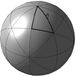
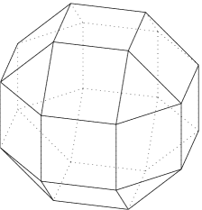
Figure 1: Tessellation of $\mathbb{S}^{2}$ for ${\cal R}={\cal O}$ and the Archimedean polyhedron ${\cal Q}_{\cal O}$.

Each vertex of such triangles corresponds to a pole $p\in{\cal P}=\Gamma\cap\mathbb{S}^{2}$. Let us select one triangle, say $\tau$. By a suitable choice of a point $q\in\partial\tau$ (see Figure 1) we can define an Archimedean polyhedron ${\cal Q}_{\cal R}$, which is the convex hull of the orbit of $q$ under ${\cal R}$, and therefore it is strictly related to the symmetry group ${\cal R}$. For details see [13].

We can characterize a cone ${\cal K}$ by a periodic sequence $\mathfrak{t}=\{\tau_{k}\}_{k\in\mathbb{Z}}$ of triangles of the tessellation such that $\tau_{k+1}$ shares an edge with $\tau_{k}$ and $\tau_{k+1}\neq\tau_{k-1}$ for each $k\in\mathbb{Z}$. This sequence is uniquely determined by ${\cal K}$ up to translations, and describes the homotopy class of the admissible paths followed by the generating particle (see Figure 2, left).

We can also characterize ${\cal K}$ by a periodic sequence $\nu=\{\nu_{k}\}_{k\in\mathbb{Z}}$ of vertexes of ${\cal Q}_{\cal R}$ such that the segment $[\nu_{k},\nu_{k+1}]$ is an edge of ${\cal Q}_{\cal R}$ and $\nu_{k+1}\neq\nu_{k-1}$ for each $k\in\mathbb{Z}$. Also the sequence $\nu$ is uniquely determined by ${\cal K}$ up to translations, and with it we can construct a piecewise linear loop $v$, joining consecutive vertexes $\nu_{k}$ with constant speed, that represents a possible motion of the generating particle (see Figure 2, right).

             

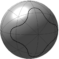
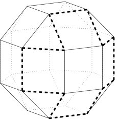
Figure 2: Encoding a cone ${\cal K}$. Left: the dashed path on $\mathbb{S}^{2}$ describes the periodic sequence $\mathfrak{t}$ of triangles of the tessellation. Right: the dashed piecewise linear path describes the corresponding periodic sequence $\nu$ of vertexes of ${\cal Q}_{\cal O}$.

The existence of a minimizer $u^{*}_{I}$ of ${\cal A}$ restricted to a cone ${\cal K}={\cal K}(\nu)$ can be shown by standard methods of calculus of variations, provided that

$$\bigcap_{\tau_{j}\in\mathfrak{t}}\overline{\tau_{j}}=\emptyset,$$ (5)

where $\mathfrak{t}$ is the sequence of spherical triangles corresponding to ${\cal K}$. Condition (5) means that the trajectory of the generating particles does not wind around one rotation axis only: this ensures the coercivity of the action functional and therefore a minimizer exists.

For later use we introduce the following definitions.

Definition 1.

We say that a cone ${\cal K}$ is ‘simple’ if the corresponding sequence $\mathfrak{t}$ does not contain a string $\tau_{k}\ldots\tau_{k+2\mathfrak{o}}$ such that

$$\bigcap_{j=0}^{2\mathfrak{o}}\overline{\tau_{k+j}}=p,$$

where $p\in\cal P$ and $\mathfrak{o}$ is the order of $p$.

Definition 2.

We say that a cone ${\cal K}$ winds around two coboundary axes if

• the corresponding sequence $\mathfrak{t}$ is the union of two strings, $\tau_{k_{j}}\ldots\tau_{k_{j}+2\mathfrak{o}_{j}}$, $j=1,2$, such that

  $$\bigcap_{h=0}^{2\mathfrak{o}_{j}}\overline{\tau_{k_{j}+h}}=p_{j},$$

  where $\mathfrak{o}_{j}$ is the order of $p_{j}$, for two different poles $p_{1},p_{2}$;

• there exists $\tau_{k}\in\mathfrak{t}$ such that $p_{1},p_{2}\in\overline{\tau_{k}}$.

To show that for a suitable choice of ${\cal K}$ the minimizers are collision-free we consider total and partial collisions separately.

2.2 Total collisions

We note that a total collision of the $N$ particles occurs at time $t_{c}$ iff $u_{I}(t_{c})=0$. If there is a total collision then, by condition (c), there are $M$ of them per period. For a minimizer $u^{*}_{I}$ with a total collision we can give the following a priori estimate for the action (see [13, Section 5]):

$${\cal A}(u^{*}_{I})\geq\alpha_{\cal R,M},$$ (6)

where $\alpha_{\cal R,M}$ depends only on $M$ and $T$. Rounded values of $\alpha_{\cal R,M}$ for $T=1$ are given in Table 1.

${\cal R}$$\diagdown$$M$	1	2	3	4	5
${\cal T}$	$132.695$	$210.640$	$276.017$	/	/
${\cal O}$	$457.184$	$725.734$	$950.981$	$1152.032$	/
${\cal I}$	$2296.892$	$3646.089$	$4777.728$	/	$6716.154$

Table 1: Lower bounds $a_{{\cal R},M}$ for loops with $M$ total collisions ($T=1$).

For some sequences $\nu$, the action of the related piecewise linear loop $v$ is lower than $\alpha_{\cal R,M}$. Therefore, minimizing the action over the cones $\cal K$ defined by such sequences yields minimizers without total collisions. The action of the piecewise linear loop $v$ can be computed explicitly and it is given by

$${\cal A}(v)=\frac{3}{2\cdot 4^{1/3}}N\ell^{2/3}(k_{1}\zeta_{1}+k_{2}\zeta_{2})^{2/3},$$ (7)

where $k_{1},k_{2}$ are the numbers of sides of the two different kinds (i.e. separating different pairs of polygons) in the trajectory of $v$, $\ell$ is the length of the sides (assuming ${\cal Q}_{\cal R}$ is inscribed in the unit sphere) and $\zeta_{1},\zeta_{2}$ are the values of explicitly computable integrals, see Table 2. Relations (6) and (7) will be useful later in Section 2

${\cal R}$	${\cal T}$	${\cal O}$	${\cal I}$
$\ell$	$1.0$	$0.7149$	$0.4479$
$\zeta_{1}$	$9.5084$	$20.3225$	$53.9904$
$\zeta_{2}$	$9.5084$	$19.7400$	$52.5762$

Table 2: Numerical values of $\ell$, $\zeta_{1}$, $\zeta_{2}$.

2.3 Partial collisions

Because of the symmetry a partial collision occurs at time $t_{c}$ iff $u_{I}(t_{c})\in\Gamma\setminus\{0\}$, that is when the generating particle passes through a rotation axis $r$. Indeed, in this case all the particles collide in separate clusters, each containing as many particles as the order of $r$. We summarize below the technique used in [13] to deal with partial collisions. We can associate to a partial collision two unit vectors $\mathsf{n}^{+},\mathsf{n}^{-}$, orthogonal to the collision axis $r$, corresponding to the ejection and collision limit directions respectively. By means of these vectors we can define a collision angle $\theta$ and, assuming that $\cal K$ is simple, we have

$$-\frac{\pi}{\mathfrak{o}_{r}}\leq\theta\leq 2\pi,$$

where $\mathfrak{o}_{r}$ is the order of the maximal cyclic group related to the collision axis $r$. If $\theta\neq 2\pi$ we can exclude partial collisions by local perturbations, constructed by using either direct or indirect arcs [9], and with a blow up technique [12]. If $\theta=2\pi$, then

• $\mathsf{n}^{+}=\mathsf{n}^{-}$,

• the plane $\pi_{r,\mathsf{n}}$ generated by $r$ and $\mathsf{n}=\mathsf{n}^{\pm}$ is fixed by some reflection $\tilde{R}\in\tilde{\cal R}$,

and we say that the partial collision is of type $(\rightrightarrows)$. In this case we cannot exclude the singularity by a local perturbation because the indirect arc is not available. However, it turns out that in this case the trajectory of the generating particle must lie on a reflection plane, bouncing between two coboundary rotation axes.

We conclude that, provided that $\cal K$ is simple and it does not wind around two coboundary axes, the minimizer $u^{*}_{I}$ of the action ${\cal A}$ restricted to ${\cal K}$ is free of partial collision, hence it is a smooth periodic solution of the $N$-body problem.

3 Enumerating all the collision-free minimizers

Here we introduce an algorithm to generate all the sequences $\nu$ of length $l$, for some admissible integer $l$. Then we select only the periodic ones, and control whether they satisfy all the conditions ensuring the existence of collision-free minimizers of (3) in the corresponding cone ${\cal K}={\cal K}(\nu)$. Precisely, our algorithm is based on the following steps:

1. Find the maximal admissible length $l_{\text{max}}$ and other constraints on the length $l$.

2. Construct all the periodic sequences $\nu$ of vertexes of the Archimedean polyhedron $\mathcal{Q}_{\mathcal{R}}$.

3. Exclude the sequences that wind around one axis only or around two coboundary axes.

4. Exclude the sequences that do not respect the additional choreography symmetry (2).

5. Exclude the sequences that give rise to non simple cones.

3.1 Constraints on the length

To exclude total collisions we use (6) and (7). If $v$ is the piecewise linear loop defined by the sequence $\nu$, the relation ${\cal A}(v)<\alpha_{\mathcal{R},M}$ can be rewritten as

$$k_{1}\zeta_{1}+k_{2}\zeta_{2}<\bigg{(}\alpha_{\mathcal{R},M}\frac{2\cdot 4^{1/3}}{3T^{1/3}}\frac{1}{N}\frac{1}{\ell^{2/3}}\bigg{)}^{3/2}:=K.$$ (8)

Since the coefficients $\zeta_{1}$ and $\zeta_{2}$ are positive, for each $M$ there exist only a finite number of positive integers $(k_{1},k_{2})$ fulfilling (8). Given ${\cal R}\in\{{\cal T},{\cal O},{\cal I}\}$, taking the maximal value of $k_{1}+k_{2}$ we get a constraint on the maximal length $l_{\text{max}}=l_{\text{max}}(M)$ of the sequence $\nu$, see Table 3.

${\cal R}$$\diagdown$$M$	1	2	3	4	5
${\cal T}$	$4$	$8$	$12$	/	/
${\cal O}$	$6$	$12$	$19$	$25$	/
${\cal I}$	$10$	$21$	$32$	/	$54$

Table 3: Values of $l_{\text{max}}(M)$ for the different symmetry groups.

On the other hand, we can also give a constraint on the minimal length $l_{\rm min}$. In fact, a periodic sequence of length $l\leq 5$ either winds around one axis only or encloses two coboundary axes. However, for all the five Platonic polyhedra there exists at least a good sequence $\nu$ of length $6$: for this reason we set $l_{\rm min}=6$.

Furthermore, in the case of $\mathcal{R}=\mathcal{T},\mathcal{O}$ we cannot have $M=1$. In fact:

• if $\mathcal{R}=\mathcal{T}$, $l_{\text{max}}(1)=4$, therefore we cannot construct any good sequence $\nu$.

• if $\mathcal{R}=\mathcal{O}$, $l_{\text{max}}(1)=6$, and the only sequences of length $6$ that do not wind around two coboundary axes have $M=2$.

3.2 Periodic sequences construction

To know which vertexes are reachable from a fixed vertex $V_{j}$ of $\mathcal{Q}_{\mathcal{R}}$, we interpret the polyhedron as a connected graph: in this manner we have an adjacency matrix $A$ associated to the graph. In this matrix we want to store the information about the kind of sides connecting two different vertexes. The generic entry of $A$ is

$$A_{ij}=\begin{cases}1&\text{if the vertex $i$ and the vertex $j$ are connected by a side of type 1},\\ 2&\text{if the vertex $i$ and the vertex $j$ are connected by a side of type 2},\\ 0&\text{otherwise.}\end{cases}$$ (9)

For a fixed length $l\in\{l_{\rm min},\dots,l_{\rm max}\}$, we want to generate all the sequences of vertexes with that length, starting from vertex $1$. Because of the symmetry, we can select the first side arbitrarily, while in the other steps we can choose only among $3$ different vertexes, since we do not want to travel forward and backward along the same side. Therefore, the total number of sequences with length $l$ is $3^{l-1}$. To generate all these different sequences we produce an array of choices $c=(c_{1},\dots,c_{l})$ such that $c_{1}=1$ and $c_{j}\in\{1,2,3\},j=2,\dots,l$. Each entry tells us the way to construct the sequence: if $v_{1},v_{2},v_{3}$ are the number of the vertexes reachable from $\nu_{j}$ (with $v_{i}$ sorted in ascending order), then $\nu_{j+1}=v_{c_{j}}$. All the different $3^{l-1}$ arrays of choices can be generated using an integer number $k\in\{0,\dots,3^{l-1}-1\}$, through its base $3$ representation.

3.3 Winding around one axis only or two coboundary axes

To check whether a closed sequence winds around one axis only we have to take into account the type of Archimedean polyhedron $\mathcal{Q}_{\mathcal{R}}$. In the cases $\mathcal{R}=\mathcal{T},\mathcal{O}$ it is sufficient to count the number $m$ of different vertexes appearing in $\nu$. If $m=3,4$ then $\nu$ winds around one axis only. The case of $\mathcal{R}=\mathcal{I}$ is different, since also pentagonal faces appear. If $m=5$, to check this property we can take the mean of the coordinates of the touched vertexes and control whether it coincides with a rotation axis or not.

We note that for $M$ different from $1$, a periodic sequence satisfying the choreography condition (10), introduced in the next paragraph, cannot wind around two coboundary axes. For this reason we decided to avoid performing this additional control, since $M=1$ is possible only in the case of $\mathcal{R}=\mathcal{I}$. In this case we exclude the non-admissible sequences in a non-automated way, looking at them one by one. We point out that such a sequence can be of three different types:

1. a pentagonal face and a triangular face sharing a vertex;

2. a pentagonal face and a square face sharing a side;

3. a square face and a triangular face sharing a side.

The sequences that travel along the boundary of two square faces sharing a vertex winds around two axes too, but these axes are not coboundary, thus we have to keep them.

3.4 Choreography condition

Condition (2) is satisfied if and only if there exists a rotation $R\in\mathcal{R}$ such that

$$\eta_{R}\nu_{j}=\nu_{j+k},$$ (10)

for some integer $k$, where $\eta_{R}$ denotes the permutation of the vertexes of $\mathcal{Q}_{\mathcal{R}}$ induced by $R$. To check condition (10), we have to construct $\eta_{R}$. Let $V_{1},\dots,V_{N}\in\mathbb{R}^{3}$ be the coordinates of all the vertexes of $\mathcal{Q}_{\mathcal{R}}$: since each rotation $R$ leaves $\mathcal{Q}_{\mathcal{R}}$ unchanged, it sends vertexes into vertexes. Therefore, we construct the matrices $\eta_{R}$ such that

$$(\eta_{R})_{ji}=\begin{cases}1&\text{if }RV_{i}=V_{j},\\ 0&\text{otherwise}.\end{cases}$$

It results that each $\eta_{R}\in\mathbb{R}^{N\times N}$ is a permutation matrix. The product of $\eta_{R}$ with the vector $\textbf{v}=(1,\dots,N)^{T}$ provides the permutation of $\{1,\dots,N\}$. At this point, given a rotation $R$, we are able to write the permuted sequence $\eta_{R}\nu$: we can simply check that (10) holds by comparing the sequences $\nu$ and $\eta_{R}\nu$. Moreover, if the condition is satisfied, we compute the value $M=k_{\nu}/k$, where $k_{\nu}$ is the minimal period of $\nu$.

3.5 Simple cone control

Definition 1 of simple cones is given by using the tessellation of the sphere induced by the reflection planes of the Platonic polyhedra. To decide whether a cone ${\cal K}$ is simple or not, we must translate this definition into a condition on the sequence of vertexes. We observe that the only way to produce a non-simple cone is by traveling all around the boundary of a face $\mathcal{F}$ of $\mathcal{Q}_{\mathcal{R}}$: for the cone ${\cal K}$, being simple or not depends on the order of the pole associated to $\mathcal{F}$ and on the way the oriented path defined by $\nu$ gets to the boundary of $\mathcal{F}$ and leaves it. We discuss first the case of a triangular face, pointing out that it is associated to a pole $p$ of order three. Suppose that $\nu$ contains a subsequence $[\nu_{k},\,\nu_{k+1},\,\nu_{k+2},\,\nu_{k+3}]$ that travels all around a triangular face $\mathcal{F}$, that is $\nu_{k}=\nu_{k+3}$. Let $\nu_{k-1}$ and $\nu_{k+4}$ be the vertexes before and after accessing the boundary of $\mathcal{F}$. Four different cases can occur:

• $\nu_{k+4}$ is a vertex of the triangular face $\mathcal{F}$ (Fig. 3, top left);

• the path defined by $\nu$ accesses and leaves $\mathcal{F}$ through the same side, i.e. $[\nu_{k-1},\nu_{k}]=[\nu_{k+3},\nu_{k+4}]$ (Fig. 3, top right);

• the path defined by $\nu$ accesses and leaves $\mathcal{F}$ through two different sides describing an angle $\theta>\pi$ around $p$ (Fig. 3, bottom left);

• the path defined by $\nu$ accesses and leaves $\mathcal{F}$ through two different sides describing an angle $\theta<\pi$ around $p$ (Fig. 3, bottom right).

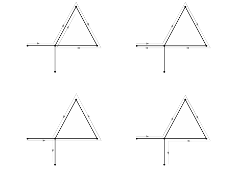
Figure 3: The different cases occurring for a path around a triangular face of $\mathcal{Q}_{\mathcal{R}}$.

In the first three cases, the sequence $\nu$ defines a non-simple cone, while case iv) is the only admissible situation for a simple cone. Cases iii) and iv) can be distinguished by the sign of $\vec{a}\times\vec{d}\cdot\vec{b}\times\vec{c}$ where

$$\vec{a}=[\nu_{k-1},\nu_{k}],\quad\vec{b}=[\nu_{k},\nu_{k+1}],\quad\vec{c}=[\nu_{k+2},\nu_{k+3}],\quad\vec{d}=[\nu_{k+3},\nu_{k+4}].$$

If this sign is positive we have case iii), if negative case iv). This argument concludes the discussion about triangular faces. Actually, we can see that the same argument can be used for square and pentagonal faces, provided that the associated poles have order greater than two. However, in the case $\mathcal{R}=\mathcal{O}$, we can find poles of order two associated to square faces. In this situation there is no way to travel all around the square face and get a simple cone.

3.6 Summary of the procedure

Now we summarize the procedure that we adopt. For each admissible value of $M$ (see Table 1) we observe that $M$ divides the possible lengths $l\in\{l_{\rm min},\dots,l_{\text{max}}(M)\}$ of the sequence $\nu$. Then, for each integer $h\in\{0,\dots,3^{l/M-1}-1\}$ we perform the following steps:

1. construct the array of choices $c$ corresponding to $h$;

2. generate the sequence $\hat{\nu}$ on the basis of $c$, starting from vertex number $1$. Note that $\hat{\nu}$ is a sequence with length $l/M+1$;

3. control whether $\eta_{R}\hat{\nu}_{1}=\hat{\nu}_{l/M+1}$ for some $R\in\mathcal{R}$. In this case we extend $\hat{\nu}$ to a sequence $\nu$ with length $l+1$, using the choreography condition (10);

4. check whether $\nu$ is periodic or not;

5. compute the minimal period $k_{\nu}$ of $\nu$;

6. check whether $\nu$ winds around one axis only or not;

7. check whether (10) holds or not; if it holds, check whether the ratio $k_{\nu}/k$ is equal to $M$ or not;

8. compute the values of $k_{1},k_{2}$ and check whether (8) holds or not;

9. check whether the cone ${\cal K}={\cal K}(\nu)$ is simple or not.

If the sequence $\nu$ passes all the controls above, then there exists a collision-free minimizer of the action ${\cal A}$ restricted to ${\cal K}$.

3.7 Results

The lists of good sequences found by the algorithm described in Section 3.6 for the three groups ${\cal T}$, ${\cal O}$, ${\cal I}$ are available at [11]. Here we list only the total number of good sequences (i.e. leading to collision-free minimizers and then classical periodic orbits) for the different polyhedra, in Table 4.

$M$	Total number
$2$	$3$
$3$	$6$
	$9$

$M$	Total number
$2$	$24$
$3$	$18$
$4$	$15$
	$57$

$M$	Total number
$1$	$28$
$2$	$386$
$3$	$455$
$5$	$573$
	$1442$

Table 4: Total number of sequences $\nu$ found for $\mathcal{Q}_{\mathcal{T}},\mathcal{Q}_{\mathcal{O}},\mathcal{Q}_{\mathcal{I}}$ respectively, from the left to the right.

All the periodic orbits listed in [13] were found again with this procedure.

We point out that we can identify two different sequences $\nu,\tilde{\nu}$ if there exists a symmetry $S$ of the polyhedron $\mathcal{Q}_{\mathcal{R}}$ such that $\eta_{R}\nu=\tilde{\nu}$, where $\eta_{R}$ still denotes the permutation of the vertexes induces by the symmetry $S$. The results are presented using this identification.

4 Numerical computation of the orbits

We describe the procedure that we have used to compute the periodic orbits described in the previous sections. Given the sequence $\nu$, first we search for a Fourier polynomial approximating the minimizer of the action functional ${\cal A}$ in ${\cal K}={\cal K}(\nu)$. Then we refine the approximation by a multiple shooting method that takes into account the symmetry of the orbit.

4.1 Approximation with Fourier polynomials

Following [22] and [25], we want to find an approximation of the motion minimizing the action functional ${\cal A}$. To discretize the infinite dimensional set of $T$-periodic loops, we take into account the truncated Fourier series at some order $F_{M}$. We consider only loops $u:[0,T]\to\mathbb{R}^{3}$ of the form

$$u(t)=\frac{a_{0}}{2}+\sum_{k=1}^{F_{M}}\bigg{[}a_{k}\cos\bigg{(}\frac{2\pi k}{T}t\bigg{)}+b_{k}\sin\bigg{(}\frac{2\pi k}{T}t\bigg{)}\bigg{]},$$ (11)

where $a_{k},b_{k}\in\mathbb{R}^{3}$ are the Fourier coefficients. Restricting ${\cal A}$ to loops of the form (11) we obtain a function $A:\mathbb{R}^{3(2F_{M}+1)}\to\mathbb{R}$ that discretizes the action functional. This function is defined (neglecting the constant factor $N$) by

$$A(a_{0},a_{1},\dots,a_{F_{M}},b_{1},\dots,b_{F_{M}})=\int_{0}^{T}\bigg{(}\frac{1}{2}\lvert\dot{u}\rvert^{2}+U(u)\bigg{)}dt,$$ (12)

where

$$U(u)=\frac{1}{2}\sum_{R\in{\cal R}\setminus\{I\}}\frac{1}{|(R-I)u|}.$$

The derivatives with respect to the Fourier coefficients are

$$\frac{\partial A}{\partial a_{k}}=\frac{2(\pi k)^{2}}{T}a_{k}+\int_{0}^{T}\frac{\partial U}{\partial u}(u(t))\cos\bigg{(}\frac{2\pi k}{T}t\bigg{)}dt,\quad k\geq 0,$$ (13)

$$\frac{\partial A}{\partial b_{k}}=\frac{2(\pi k)^{2}}{T}b_{k}+\int_{0}^{T}\frac{\partial U}{\partial u}(u(t))\sin\bigg{(}\frac{2\pi k}{T}t\bigg{)}dt,\quad k>0.$$ (14)

Note that these derivatives may be large for high frequencies because of the term $k^{2}$, and this leads to an instability of the classical gradient method (see [22]). In [22] the authors propose a variant of the gradient method avoiding this problem. If $a_{k}$ is the $k$-th Fourier coefficient at some iteration, we obtain the new coefficient $a_{k}^{\prime}$ for the successive step by adding

$$\delta a_{k}=a_{k}^{\prime}-a_{k}=-\delta\tau_{k}\frac{\partial A}{\partial a_{k}},$$ (15)

and similarly for the coefficients $b_{k}$. This means that the decay rate in the Fourier coefficients is controlled by a parameter $\delta\tau_{k}$ which depends also on the order $k$ of the harmonic. If we set

$$\delta\tau_{k}=\frac{T}{2(\pi k)^{2}}\delta,$$ (16)

where $\delta>0$ is a small positive constant, this removes the high frequency instability.

To stop the iterations we could check the value of the residual acceleration, i.e. the difference between the acceleration computed from $u(t)$ and the force acting on the generating particle at time $t$. However, this in practice can be done only when there are no close encounters between the bodies. In fact, when a passage near a collision occurs, we have to choose a very large value of $F_{M}$ (see [25]) to obtain a better approximation, and this slows down the computations. For this reason we choose to stop the iterations also when the increments $\delta a_{k},\delta b_{k}$ become small, as suggested in [22].

4.2 Shooting method

In order to refine the computation of the orbits, we use a shooting method in the phase space of the generating particle, starting from the Fourier polynomial approximations. The goal is to solve the problem

$$\begin{cases}\dot{x}=f(x),\\ x(T/M)=Sx(0),\end{cases}$$ (17)

where $x=(u,\dot{u})\in\mathbb{R}^{6}$, $S$ is the matrix

$$S=\begin{pmatrix}R&0\\ 0&R\end{pmatrix},$$

with $R\in\mathcal{R}$ and $M>0$ given by condition (c). The differential equation in (17) comes from the Euler-Lagrange equation of the functional defined by (3). Fixed $n$ points $0=\tau_{0}<\tau_{1}<\cdots<\tau_{n}=T/M$, we define the function $G:\mathbb{R}^{6n}\to\mathbb{R}^{6n}$ as

$$\begin{cases}G_{i}=\phi^{\tau_{i}-\tau_{i-1}}(x_{i-1})-x_{i},&i=1,\dots,n-1\\ G_{n}=\phi^{\tau_{n}-\tau_{n-1}}(x_{n-1})-Sx_{0},\end{cases}$$ (18)

where the points $x_{i}=(u(\tau_{i}),\dot{u}(\tau_{i}))$ correspond to a discretization of the position and velocity of the generating particle, modeled with the Fourier polynomial approximation. If we have a $T$-periodic solution $x(t)$ satisfying (17), the function $G$ evaluated at

$$X=(x(\tau_{0}),\dots,x(\tau_{n-1}))$$

vanishes. To search for the zeros of $G$ we use a least-squares approach: we set

$$F(X)=\frac{|G(X)|^{2}}{2},$$

and search for the absolute minimum points by a modified Newton method. The derivatives of $F$ are

$$\frac{\partial F}{\partial x_{j}}=\sum_{i=1}^{n}\frac{\partial G_{i}}{\partial x_{j}}\cdot G_{i},$$ (19)

$$\frac{\partial^{2}F}{\partial x_{j}\partial x_{h}}=\sum_{i=1}^{n}\bigg{[}\frac{\partial G_{i}}{\partial x_{j}}\frac{\partial G_{i}}{\partial x_{h}}+\frac{\partial^{2}G_{i}}{\partial x_{j}\partial x_{h}}G_{i}\bigg{]}.$$ (20)

The Jacobian matrix of $G$ is

$$\begin{bmatrix}M_{1}&-\operatorname{Id}&&\\ &M_{2}&\ddots&&\\ &&\ddots&-\operatorname{Id}\\ -S&&&M_{n}\end{bmatrix},$$ (21)

where

$$M_{i}=\frac{\partial}{\partial x}\phi^{\tau_{i}-\tau_{i-1}}(x_{i}).$$

If $X^{\prime}$ denotes the new value of $X$ at some iteration of the modified Newton method and $\Delta X=X^{\prime}-X$, at each step we solve the linear system

$$A(X)\Delta X=-\frac{\partial F}{\partial X}(X),$$ (22)

where the entries of the matrix $A$ are

$$A_{jh}=\sum_{i=1}^{n}\frac{\partial G_{i}}{\partial x_{j}}\frac{\partial G_{i}}{\partial x_{h}},$$

i.e. we consider only an approximation of the second derivatives (20) of $F$. However, $A$ is singular at the minimum points, since we are free to choose the initial point along the periodic orbits. This degeneracy can be avoided as in [1], by adding the condition on the first shooting point

$$f(x_{0})\cdot\Delta x_{0}=0,$$ (23)

to (22), where $x_{0},\Delta x_{0}$ are the first components of $X,\Delta X$. The system of equations (22), (23) has $6n+1$ equations and $6n$ unknowns, and we can solve it through the SVD decomposition, thus obtaining the value of $\Delta X$. We have performed the integration of the equation of motion and of the variational equation with both the DOP853 and the RADAU IIA integrators, available at [15].

5 Linear stability

We study the stability of the orbit of the generating particle, whose dynamics is defined by (17). This corresponds to study the stability of the periodic orbit of the full $N$-body problem with respect to symmetric perturbations. However, if the orbit of the generating particle is unstable, also the full orbit of $N$-body is unstable.

From the standard Floquet theory we know that the monodromy matrix $\mathfrak{M}(T)$ is a $6\times 6$ real symplectic matrix with a double unit eigenvalue, one arising from the periodicity of the orbit and the other one from the energy conservation. Since $\mathfrak{M}(T)$ is symplectic, we have only three possibilities for the remaining eigenvalues $\lambda_{1},\lambda_{2},\lambda_{3},\lambda_{4}$:

1. some of them are real and $\lambda_{1}\lambda_{2}=1,\lambda_{3}\lambda_{4}=1$;

2. $\lambda_{1},\lambda_{2},\lambda_{3},\lambda_{4}\in\mathbb{C}\setminus\mathbb{R}$ and $\lambda_{1}=\lambda_{2}^{-1}=\bar{\lambda}_{3}=\bar{\lambda}_{4}^{-1}$;

3. $\lambda_{1},\lambda_{2},\lambda_{3},\lambda_{4}\in\mathbb{C}\setminus\mathbb{R}$ and $\lambda_{1}=\lambda_{2}^{-1}=\bar{\lambda}_{2},\lambda_{3}=\lambda_{4}^{-1}=\bar{\lambda}_{4}$.

As in [17], we can give a stability criterion using the values $T_{1}=\lambda_{1}+\lambda_{2}$ and $T_{2}=\lambda_{3}+\lambda_{4}$. The characteristic polynomial of the monodromy matrix is

$$\begin{split}p(\lambda)&=(\lambda-1)^{2}(\lambda-\lambda_{1})(\lambda-\lambda_{2})(\lambda-\lambda_{3})(\lambda-\lambda_{4})\\ &=(\lambda-1)^{2}(\lambda^{2}-T_{1}\lambda+1)(\lambda^{2}-T_{2}\lambda+1)\\ &=\lambda^{6}-(T_{1}+T_{2}+2)\lambda^{5}+(T_{1}T_{2}+2(T_{1}+T_{2})+3)\lambda^{4}+\dots\end{split}.$$

Let us denote by $d_{ij}$ the generic entry of the monodromy matrix, and set

$$a=\sum_{i=1}^{6}d_{ii},\qquad b=\sum_{1\leq i\leq j\leq 6}(d_{ii}d_{jj}-d_{ij}d_{ji}).$$

From the expressions of the coefficients of the characteristic polynomial we obtain

$$\begin{cases}T_{1}+T_{2}+2=a,\\ T_{1}T_{2}+2(T_{1}+T_{2})+3=b.\end{cases}$$ (24)

It turns out that $T_{1}$ and $T_{2}$ are the roots of the polynomial of degree two

$$q(s)=s^{2}-(a-2)s+(b-2a+1).$$ (25)

We use the following result, see [17].

Lemma 1.

Let $T_{1},T_{2}$ the roots of the polynomial (25). The eigenvalues of the monodromy matrix lie on the unit circle if and only if

$$\begin{cases}\Delta=(a-2)^{2}-4(b-2a+1)>0,\\ \lvert T_{1}\rvert<2,\quad\lvert T_{2}\rvert<2.\end{cases}$$ (26)

Proof.

The hypothesis $\Delta>0$ yields that $T_{1},T_{2}$ are real and distinct. This excludes condition $2)$ above. We also exclude condition $1)$, because in this case we have

$$\lvert T_{1}\rvert=\lvert\lambda_{1}+\lambda_{2}\rvert=\lvert\lambda_{1}+\lambda_{1}^{-1}\rvert>2,\quad\lvert T_{2}\rvert=\lvert\lambda_{3}+\lambda_{4}\rvert=\lvert\lambda_{3}+\lambda_{3}^{-1}\rvert>2.$$

The only possibility is the third, that is the eigenvalues of the monodromy matrix lie on the unit circle.

∎

By this Lemma we avoid the numerical computation of the eigenvalues and we can establish the stability of the orbit simply by computing the roots of a polynomial of degree two, whose coefficients depend only on the entries of the monodromy matrix $\mathfrak{M}(T)$.

Moreover, for symmetric periodic orbits we can factorize $\mathfrak{M}(T)$ as in [24]:

$$\mathfrak{M}(T)=(S^{T}\mathfrak{M}({T}/{M}))^{M},$$ (27)

where $\mathfrak{M}(t)$ is the fundamental solution of the variational equation at time $t$. This means that we can integrate the variational equation only over the time span $[0,T/M]$ and we can study the stability by applying Lemma 26 to the matrix $S^{T}\mathfrak{M}(T/M)$.

Our numerical computations suggest that all the periodic orbits found in Section 3 are unstable. Non rigorous numerical values of $\Delta,T_{1},T_{2}$ for several cases can be found at [11]. To make rigorous the results, we have to integrate the equation of motion using interval arithmetic ([23]), as explained in the next section.

6 Validation of the results

We use interval arithmetic to obtain rigorous estimates of the initial condition of a periodic orbit and its monodromy matrix. Using these estimates we can give a computer-assisted proof of the instability of such orbit. To integrate rigorously a system of ODEs we use the $C^{1}$-Lohner algorithm [30] implemented in the CAPD library [16], which is based on a Taylor method to solve the differential equations. Given a set of initial conditions and a final time $\tau$, this algorithm produces an enclosure of the solution and of its derivatives with respect to the initial conditions at time $\tau$.

Denoting by $(u,\dot{u})\in\mathbb{R}^{6}$ the position and the velocity of the generating particle, system (17) has the first integral of the energy

$$E(u,\dot{u})=\frac{1}{2}|\dot{u}|^{2}+\frac{1}{2}\sum_{R\in{\cal R}\setminus\{I\}}\frac{1}{|(R-I)u|}.$$

Fix the value of the energy and use a surface of section to search for the periodic orbit. More precisely, we use the Poincaré first return map

$$\mathsf{p}:\Sigma\to\Sigma,$$

with

$$\Sigma=\{(u,\dot{u})\in\mathbb{R}^{6}:u_{3}=0,\,E(u,\dot{u})=h\},$$

where $u_{3}$ is the third component of $u$ and $h$ is the value of the energy of an approximated initial condition $(u_{0},\dot{u}_{0})$. This condition is computed from the solution $\tilde{u}(t)$ obtained with the shooting method explained in Section 4.2, which is propagated to reach the plane $u_{3}=0$. Up to a rotation $R\in{\cal R}$, we can always assume that $\tilde{u}(t)$ passes through this plane.

To compute an enclosure of the initial condition we use the interval Newton method (see, for instance, [23]). Given a box $B\subset\Sigma$ around $(u_{0},\dot{u}_{0})$ we define the interval Newton operator as

$$N((u_{0},\dot{u}_{0}),B,\mathsf{f})=(u_{0},\dot{u}_{0})-[d\mathsf{f}(B)]^{-1}\mathsf{f}(u_{0},\dot{u}_{0}),$$

where $\mathsf{f}(u,\dot{u})=\mathsf{p}(u,\dot{u})-(u,\dot{u})$ and $[d\mathsf{f}(B)]$ denotes the interval enclosure of $d\mathsf{f}(B)$. If we are able to verify that

$$N((u_{0},\dot{u}_{0}),B,\mathsf{f})\subset B,$$ (28)

then from the interval Newton theorem there exists a unique fixed point in $B$ for the Poincaré map $\mathsf{p}$, and therefore a unique initial condition for the corresponding periodic orbit.

Given a box $B$ that satisfies (28), we use the $C^{1}$-Lohner algorithm to compute an enclosure for $\mathfrak{M}(T/M)$. Then, using the factorization (27), we can compute also an enclosure for the values of $\Delta,T_{1},T_{2}$ and verify whether the hypotheses of Lemma 26 hold or not.

6.1 Numerical tests

We have applied the method described above to give a rigorous proof of the instability of the periodic orbits listed in Table 5. The $N$-body motion corresponding to the selected cases is displayed in Figure 4.

label	$M$	vertexes of $\mathcal{Q}_{\mathcal{O}}$
$\nu_{1}$	$3$	$[1,3,8,10,16,5,1]$
$\nu_{16}$	$2$	$[1,3,8,18,13,12,4,9,2,19,11,14,1]$
$\nu_{27}$	$3$	$[1,3,7,20,18,8,15,4,6,10,16,5,1]$
$\nu_{43}$	$4$	$[1,3,8,15,4,9,2,5,1]$

Table 5: List of sequences used in the tests. The labels correspond to the enumeration used in the website [11].

         

         

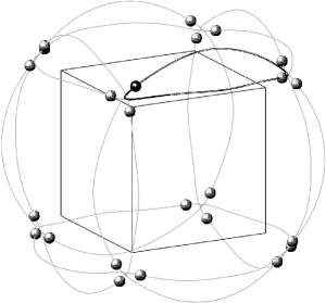
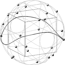
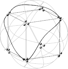
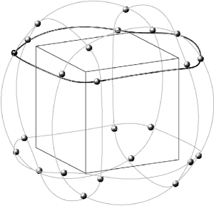
Figure 4: Periodic motions of the $N$ bodies corresponding to the sequences listed in Table 5. The solid black curve represents the trajectory of the generating particle.

Hereafter we shall use a notation similar to [17, 18] to describe an interval: first we write the digits shared by the interval extrema, then the remaining digits are reported as subscript and superscript. Thus, for instance, we write

$$12.3456789_{1234}^{5678}$$

for the interval

$$[12.34567891234,12.34567895678].$$

For the four selected cases in Table 5 we checked that condition (28) holds using multiple precision interval arithmetic. This ensures the existence of an initial condition for the orbits in the selected box $B$. When the bodies do not undergo close approaches, as in the cases of $\nu_{16}$ and $\nu_{43}$, the inclusion can be checked with a much larger box. On the other hand, when close approaches occur, as in the cases of $\nu_{1}$ and $\nu_{27}$, we are forced to use a very tiny box, a longer mantissa and a higher order for the Taylor method (see Table 6). This increases significantly the computational time. To show the instability of these orbits we prove that conditions (26) are violated. For $\nu_{16}$ and $\nu_{43}$ these computations are successful even using only double precision interval arithmetic. In the other two cases we need multiple precision and a higher order for the Taylor method. As we can see from Table 6, the value of $T_{1}$ is well above $2$, that yields a computer-assisted proof of the instability of these four test orbits. In Table 7 we report also the non-rigorous values of $\Delta,T_{1},T_{2}$, obtained by numerical integration without interval arithmetic. Comparing the values in the two tables, we can see that the non-rigorous ones are in good agreement with the estimates computed with interval arithmetic. Non-rigorous values for several other orbits can be found at [11].

label	mantissa (bits)	size($B$)	order	$\Delta$	$T_{1}$	$T_{2}$
$\stackrel{{\scriptstyle\phantom{R}}}{{\nu_{1}}}$	$100$	$2\cdot 10^{-18}$	30	$1488.95_{2965}^{3031}$	$43.365_{499}^{500}$	$4.778546_{1}^{6}$
$\stackrel{{\scriptstyle\phantom{R}}}{{\nu_{16}}}$	$52$	$2\cdot 10^{-14}$	15	$90582.1_{06}^{30}$	$301.0993_{68}^{89}$	$0.1307_{359}^{566}$
	$\stackrel{{\scriptstyle\phantom{}}}{{100}}$	$2\cdot 10^{-14}$	30	$90582.1_{14}^{22}$	$301.0993_{76}^{82}$	$0.13074_{33}^{92}$
$\stackrel{{\scriptstyle\phantom{R}}}{{\nu_{27}}}$	$100$	$2\cdot 10^{-25}$	30	$5105.47178_{6}^{7}$	$73.279035_{5}^{6}$	$1.826451_{3}^{4}$
$\stackrel{{\scriptstyle\phantom{R}}}{{\nu_{43}}}$	$52$	$2\cdot 10^{-14}$	15	$7.0355_{19}^{20}$	$9.2322605_{1}^{9}$	$6.579805_{0}^{1}$
	$\stackrel{{\scriptstyle\phantom{}}}{{100}}$	$2\cdot 10^{-14}$	30	$7.0355_{19}^{20}$	$9.2322605_{3}^{8}$	$6.579805_{0}^{1}$

Table 6: Enclosures for the values of $\Delta,T_{1},T_{2}$.

label	$\Delta$	$T_{1}$	$T_{2}$
$\nu_{1}$	$1488.953003$	$43.365500$	$4.778546$
$\nu_{16}$	$90582.118054$	$301.099379$	$0.130746$
$\nu_{27}$	$5105.471786$	$73.279035$	$1.826451$
$\nu_{43}$	$7.035519$	$9.232260$	$6.579805$

Table 7: Non rigorous values of $\Delta,T_{1},T_{2}$.

7 Conclusions and future work

Using the algorithm described in Section 3, we created a list of all the periodic orbits of the $N$-body problem whose existence can be proved as in [13], where only a few of them were listed. We also set up a procedure aimed to compute these orbits, and investigated the stability for a large number of them. All the solutions found with the rotation groups $\{\mathcal{T},\mathcal{O}\}$ appear to be unstable, with a large value of $|T_{1}|$ or $|T_{2}|$ (see the website [11] for the results). Using multiple precision interval arithmetic, we were able to make rigorous these results for a few orbits, producing a computer-assisted proof of their instability. From the numerical point of view, the main difficulty is to automatize the choice of the parameters appearing in the computations: the order of the Fourier polynomials, the number of shooting points, the size of the boxes, the order of the Taylor method, the mantissa size for multiple precision computations, etc. Moreover, when the bodies undergo close approaches a longer computational time is needed to check whether condition (28) holds, because a larger size of the mantissa is required. This requires a long computational time. For these reasons we performed interval arithmetic computations only for a few orbits in our list.

We have also to point out that there is no guarantee that the computed periodic solutions correspond to minimizers of the action ${\cal A}$, whose existence have been assessed in Sections 2, 3. Indeed, with the proposed procedure, we first search for a minimizer of ${\cal A}$ in a finite dimensional set of Fourier polynomials by a gradient method, decreasing the value of the action; then we refine these solutions by a shooting method. This algorithm is meant to obtain local minima of the action ${\cal A}$. However, there is no proof, not even computer-assisted, that the computed solutions minimize the action ${\cal A}$ in the cone ${\cal K}$. We plan to investigate this aspect in the future.

As a final remark, we observe that the procedure described in Section 6 can also be used to prove the existence of periodic orbits not included in our list. For example, the sequence

$$\nu=[1,3,7,18,20,24,12,4,9,17,19,21,23,14,1],$$

of vertexes of $\mathcal{Q}_{\mathcal{O}}$ does not satisfy the condition on the maximal length (8): in fact it has $M=2$, $l_{\text{max}}(2)=12$ and the length of $\nu$ is $14$. This means that we cannot exclude total collisions. However, the validity of condition (28) can be checked numerically. Using the approximated orbit obtained with multiple shooting, we were able to check that (28) holds using a box with size $2\cdot 10^{-14}$. In this way, we have a computer-assisted proof of the existence of a periodic orbit belonging to ${\cal K}(\nu)$, represented in Figure 5.

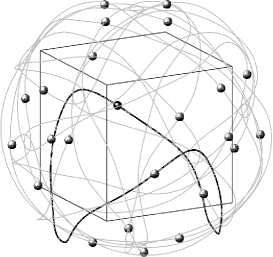
Figure 5: Periodic motion with $\nu$ not fulfilling condition (8).

We also found the values

$$\Delta=4423_{29}^{58},\quad T_{1}=665.3_{83}^{94},\quad T_{2}=0._{293}^{305},$$

that yields a rigorous proof of the instability of this orbit.

References

- [1] A. Abad, R. Barrio, and Á. Dena. Computing periodic orbits with arbitrary precision. Phys. Rev. E, 84:016701, 2011.
- [2] G. Arioli, V. Barutello, and S. Terracini. A new branch of Mountain Pass solutions for the choreographical 3-body problem. Comm. Math. Phys., 268(2):439–463, 2006.
- [3] Ugo Bessi and Vittorio Coti Zelati. Symmetries and noncollision closed orbits for planar -body-type problems. Nonlinear Anal., 16(6):587–598, 1991.
- [4] K.-C. Chen. Binary decompositions for planar -body problems and symmetric periodic solutions. Arch. Ration. Mech. Anal., 170(3):247–276, 2003.
- [5] K. C. Chen. Existence and minimizing properties of retrograde orbits to the three-body problem with various choices of masses. Annals of Mathematics, 167(2):325–348, 2008.
- [6] A. Chenciner. Action minimizing solutions of the newtonian -body problem: from homology to symmetry. In Proceedings of the International Congress of Mathematicians, Vol. III (Beijing, 2002), pages 279–294. Higher Ed. Press, Beijing, 2002.
- [7] A. Chenciner and R. Montgomery. A remarkable periodic solution of the three-body problem in the case of equal masses. Annals of Mathematics, 152(3):881–901, 2000.
- [8] A. Chenciner and A. Venturelli. Minima de l’intégrale d’action du problème newtonien de 4 corps de masses égales dans : orbites “hip-hop”. Cel. Mech. Dyn. Ast., 77(2):139–152, 2000.
- [9] Alain Chenciner. Symmetries and “simple” solutions of the classical -body problem. In XIVth International Congress on Mathematical Physics, pages 4–20. World Sci. Publ., Hackensack, NJ, 2005.
- [10] M. Degiovanni and F. Giannoni. Dynamical systems with newtonian type potentials. Ann. Scuola Norm. Sup. Pisa Cl. Sci. (4), 15(3):467–494, 1988.
- [11] M. Fenucci. http://adams.dm.unipi.it/~fenucci/research/nbody.html.
- [12] D. L. Ferrario and S. Terracini. On the existence of collisionless equivariant minimizers for the classical n-body problem. Inventiones mathematicae, 155(2):305–362, 2004.
- [13] G. Fusco, G. F. Gronchi, and P. Negrini. Platonic polyhedra, topological constraints and periodic solutions of the classical n-body problem. Inventiones mathematicae, 185(2):283–332, 2011.
- [14] W. B. Gordon. A minimizing property of Keplerian orbits. Amer. J. Math., 99(5):961–971, 1977.
- [15] E. Hairer. http://www.unige.ch/~hairer/software.html.
- [16] Computer Assisted Proofs in Dynamics (CAPD), a package for rigorous numerics. http://capd.ii.uj.edu.pl/.
- [17] T. Kapela and C. Simó. Computer assisted proofs for nonsymmetric planar choreographies and for stability of the eight. Nonlinearity, 20:1241–1255, 2007.
- [18] T. Kapela and C. Simó. Rigorous KAM results around arbitrary periodic orbits for Hamiltonian systems. Nonlinearity, 30(3):965–986, 2017.
- [19] T. Kapela and P. Zgliczynski. The existence of simple choreographies for the -body problem - a computer assisted proof. Nonlinearity, 16(6):1899–1918, 2003.
- [20] C. Marchal. How the method of minimization of action avoids singularities. Celestial Mech. Dynam. Astronom., 83(1-4):325–353, 2002. Modern celestial mechanics: from theory to applications (Rome, 2001).
- [21] C. Moore. Braids in classical dynamics. Phys. Rev. Lett., 70(24):3675–3679, 1993.
- [22] C. Moore and M. Nauenberg. New periodic orbits for the n-body problem. Journal of Computational and Nonlinear Dynamics, 1(4):307–311, 2006.
- [23] R. E. Moore, R. B. Kearfott, and M. J. Cloud. Introduction to Interval Analysis. Society for Industrial and Applied Mathematics, Philadelphia, PA, USA, 2009.
- [24] G. E. Roberts. Linear stability analysis of the figure-eight orbit in the three-body problem. Ergodic Theory and Dynamical Systems, 27:1947–1963, 2007.
- [25] C. Simó. New families of solutions in n-body problems. In Carles Casacuberta, Rosa Maria Miró-Roig, Joan Verdera, and Sebastià Xambó-Descamps, editors, European Congress of Mathematics: Barcelona, July 10–14, 2000, Volume I, pages 101–115, Basel, 2001. Birkhäuser Basel.
- [26] C. Simó. Periodic orbits of the planar -body problem with equal masses and all bodies on the same path, pages 265–284. IoP Publishing, 2001.
- [27] C. Simó. Dynamical properties of the figure eight solution of the three-body problem. In Celestial mechanics (Evanston, IL, 1999), volume 292 of Contemp. Math., pages 209–228. Amer. Math. Soc., Providence, RI, 2002.
- [28] S. Terracini. On the variational approach to the periodic -body problem. Cel. Mech. Dyn. Ast., 95:3–25, 2006.
- [29] S. Terracini and A. Venturelli. Symmetric trajectories for the -body problem with equal masses. Arch. Ration. Mech. Anal., 184(3):465–493, 2007.
- [30] P. Zgliczynski. Lohner Algorithm. Foundations of Computational Mathematics, 2(4):429–465, 2002.